Niels Tuning (1)

Particle Physics II – CP violation (also known as “Physics of Anti-matter”) Lecture 3

N. Tuning

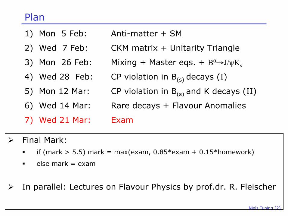
Plan 1)  Mon 5 Feb: Anti-matter + SM

2)  Wed 7 Feb: CKM matrix + Unitarity Triangle

3)  Mon 26 Feb: Mixing + Master eqs. + B0→J/ψKs

4)  Wed 28 Feb: CP violation in B(s) decays (I)

5)  Mon 12 Mar: CP violation in B(s) and K decays (II)

6)  Wed 14 Mar: Rare decays + Flavour Anomalies

7)  Wed 21 Mar: Exam

Niels Tuning (2)

Ø  Final Mark: §  if (mark > 5.5) mark = max(exam, 0.85*exam + 0.15*homework)

§  else mark = exam

Ø  In parallel: Lectures on Flavour Physics by prof.dr. R. Fleischer

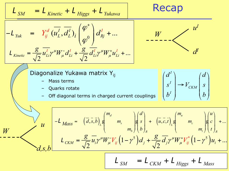
Diagonalize Yukawa matrix Yij –  Mass terms –  Quarks rotate

–  Off diagonal terms in charged current couplings

Niels Tuning (4)

Recap SM Kinetic Higgs Yukawa= + +L L L L

0( , ) ...I I

Yuk Li L Rjd Ij id dY u

ϕ

ϕ

+⎛ ⎞− = +⎜ ⎟⎜ ⎟

⎝ ⎠L

...2 2Kinetic Li Li

I I ILi L

Ii

g gu W d d W uµ µµ µγ γ− += + +L

( ) ( )5 5*1 1 ...2 2ij iCKM i j j j ig gu W d d uV VWµ µ

µ µγ γ γ γ− += − + − +L

( ) ( ), , , , ...d u

s cL L

b tR R

Mass

m d m ud s b m s u c t m c

m b m t

⎛ ⎞ ⎛ ⎞ ⎛ ⎞ ⎛ ⎞⎜ ⎟ ⎜ ⎟ ⎜ ⎟ ⎜ ⎟− = + +⎜ ⎟ ⎜ ⎟ ⎜ ⎟ ⎜ ⎟⎜ ⎟ ⎜ ⎟ ⎜ ⎟ ⎜ ⎟⎝ ⎠ ⎝ ⎠ ⎝ ⎠ ⎝ ⎠

g g g gL

I

ICKM

I

d ds V sb b

⎛ ⎞ ⎛ ⎞⎜ ⎟ ⎜ ⎟→⎜ ⎟ ⎜ ⎟

⎜ ⎟⎜ ⎟ ⎝ ⎠⎝ ⎠

SM CKM Higgs Mass= + +L L L L

uI

dI

W

u

d,s,b

W

Niels Tuning (5)

Charged Currents

( ) ( )

†

*

5 5 5 5

5 5

2 21 1 1 12 2 2 22 2

1 12 2

I I I ICC Li Li Li Li CC

ij ji

ij i

CC

i j j i

i j j ij

g gu W d d W u J W J W

g gu W d d W uV V

Vg gu W d d W uV

µ µ µ µµ µ µ µ

µ µµ µ

µ µµ µ

γ γ

γ γ γ γγ γ

γ γ γ γ

− + − − + +

− +

− +

= + = +

⎛ ⎞ ⎛ ⎞ ⎛ ⎞ ⎛ ⎞− − − −= +⎜ ⎟ ⎜ ⎟ ⎜ ⎟ ⎜ ⎟

⎝ ⎠ ⎝ ⎠ ⎝ ⎠ ⎝ ⎠

= − + −

L

( ) ( )5 * 51 12 2

CP iCC j i i jij ij

g gd W u u WV V dµ µµ µγ γ γ γ+⎯⎯→ − + −L

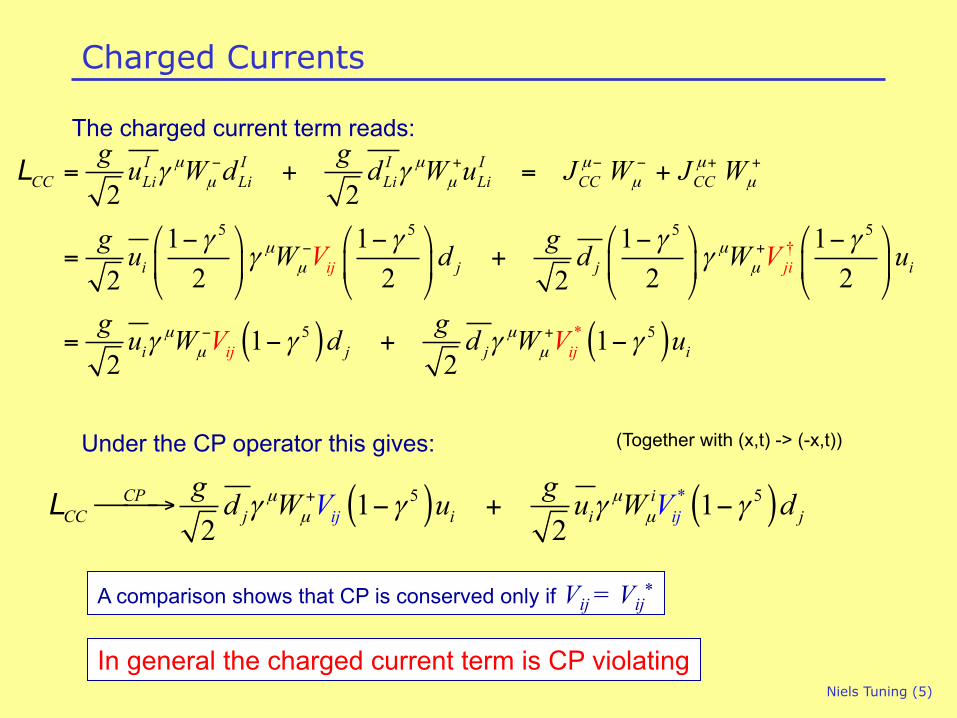
A comparison shows that CP is conserved only if Vij = Vij*

(Together with (x,t) -> (-x,t))

The charged current term reads:

Under the CP operator this gives:

In general the charged current term is CP violating

Niels Tuning (6)

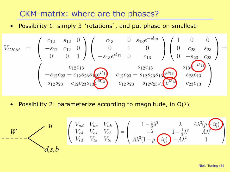
CKM-matrix: where are the phases?

u

d,s,b

W

•  Possibility 1: simply 3 ‘rotations’, and put phase on smallest:

•  Possibility 2: parameterize according to magnitude, in O(λ):

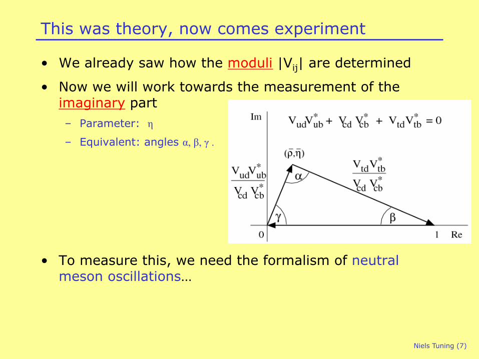
This was theory, now comes experiment

•  We already saw how the moduli |Vij| are determined

•  Now we will work towards the measurement of the imaginary part –  Parameter: η

–  Equivalent: angles α, β, γ .

•  To measure this, we need the formalism of neutral meson oscillations…

Niels Tuning (7)

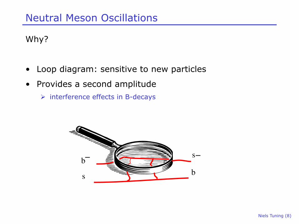
Neutral Meson Oscillations

Why?

•  Loop diagram: sensitive to new particles

•  Provides a second amplitude Ø  interference effects in B-decays

Niels Tuning (8)

b s

s

b

Niels Tuning (9)

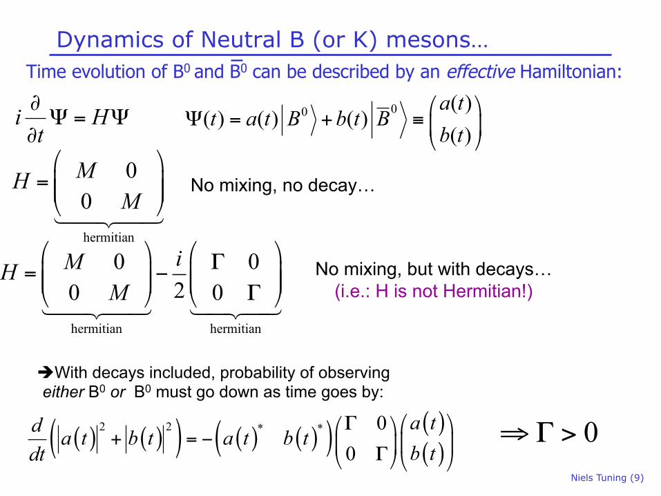
Dynamics of Neutral B (or K) mesons…

00 ( )( ) ( ) ( )

( )a t

t a t B b t Bb t⎛ ⎞

Ψ = + ≡ ⎜ ⎟⎝ ⎠

i Ht∂Ψ = Ψ

∂

H = M 00 M

!

"##

$

%&&

hermitian! "# $#

No mixing, no decay…

H = M 00 M

!

"##

$

%&&

hermitian! "# $#

−i2

Γ 00 Γ

!

"##

$

%&&

hermitian! "# $#

No mixing, but with decays… (i.e.: H is not Hermitian!)

( ) ( )( ) ( ) ( )( ) ( )( )

2 2 * * 00

a td a t b t a t b tb tdt⎛ ⎞Γ⎛ ⎞

+ = − ⎜ ⎟⎜ ⎟Γ⎝ ⎠⎝ ⎠

è With decays included, probability of observing either B0 or B0 must go down as time goes by:

0⇒Γ >

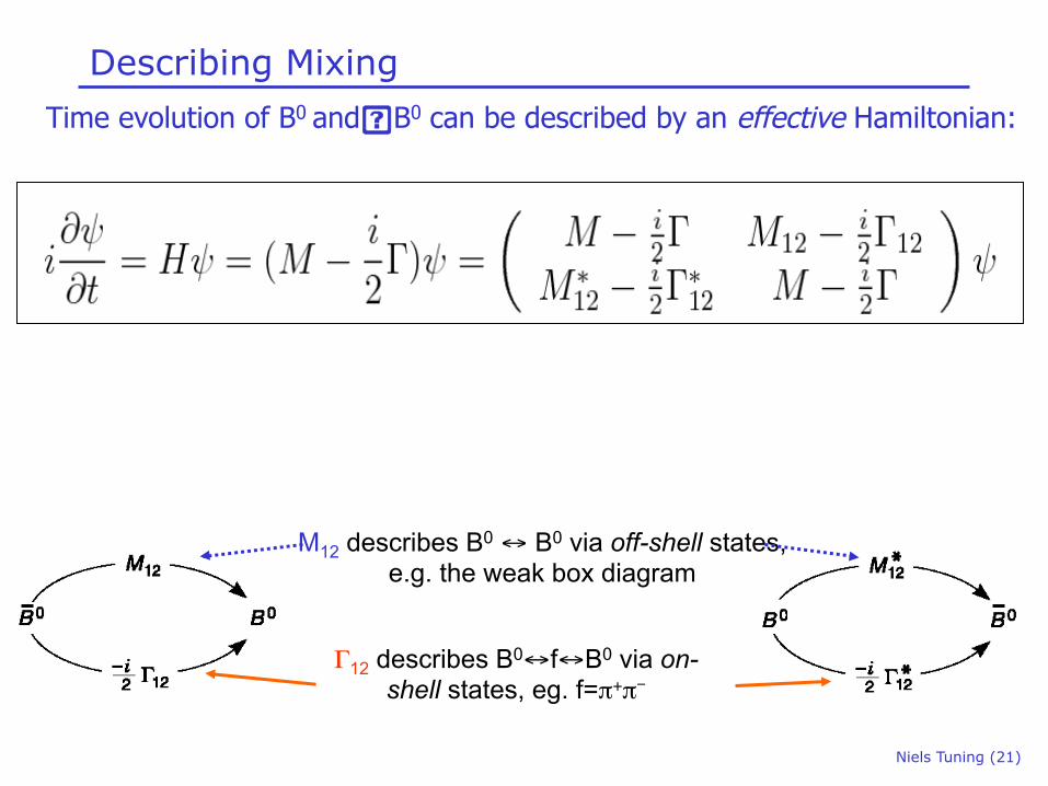
Time evolution of B0 and B0 can be described by an effective Hamiltonian:

Niels Tuning (10)

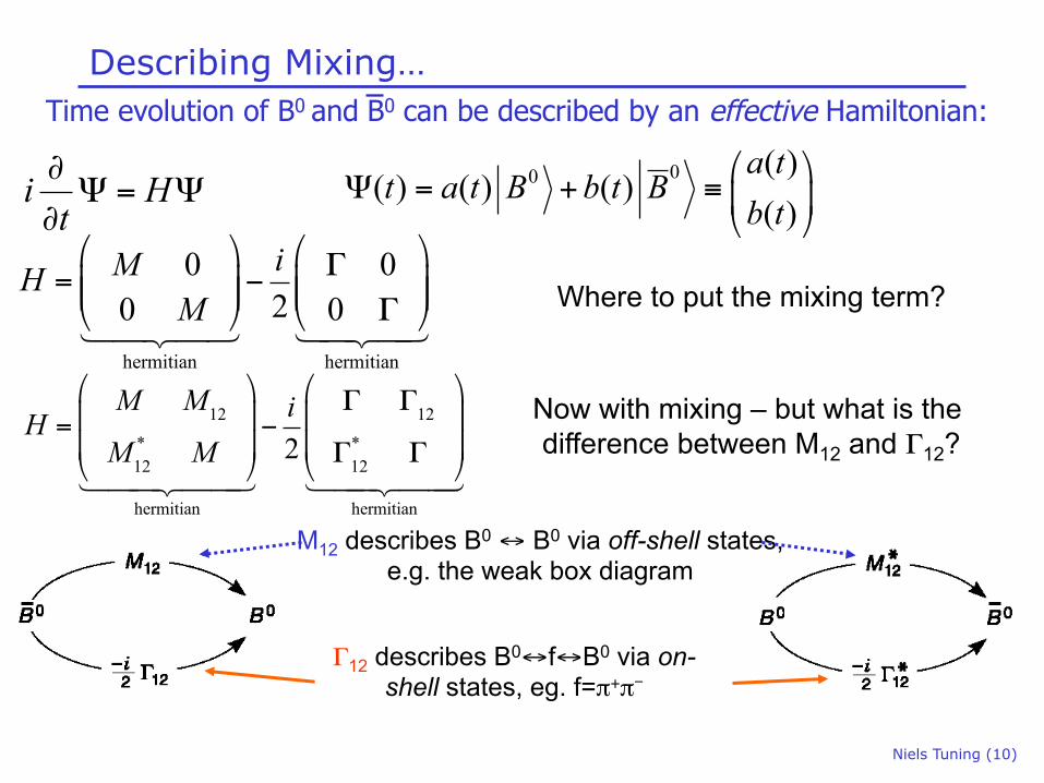
Describing Mixing…

00 ( )( ) ( ) ( )

( )a t

t a t B b t Bb t⎛ ⎞

Ψ = + ≡ ⎜ ⎟⎝ ⎠

i Ht∂Ψ = Ψ

∂

H = M 00 M

!

"##

$

%&&

hermitian! "# $#

−i2

Γ 00 Γ

!

"##

$

%&&

hermitian! "# $#

Where to put the mixing term?

H =M M12

M12* M

!

"

##

$

%

&&

hermitian! "## $##

−i2

Γ Γ12Γ12* Γ

"

#

$$

%

&

''

hermitian! "## $##

Now with mixing – but what is the difference between M12 and Γ12?

M12 describes B0 ↔ B0 via off-shell states, e.g. the weak box diagram

Γ12 describes B0↔f↔B0 via on-shell states, eg. f=π+π-

Time evolution of B0 and B0 can be described by an effective Hamiltonian:

Niels Tuning (11)

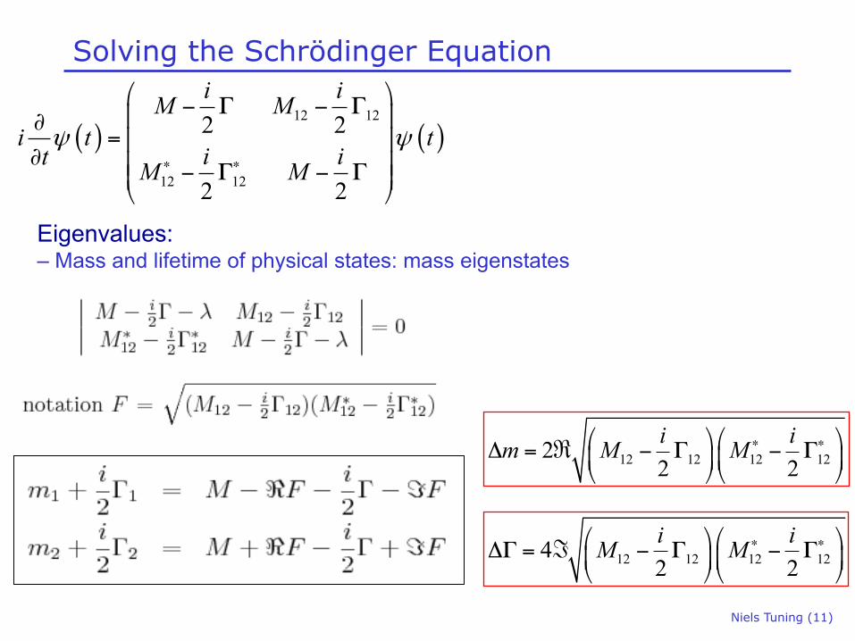
Solving the Schrödinger Equation

( ) ( )12 12

12 12

2 2

2 2

i iM Mi t t

i it M Mψ ψ

∗ ∗

⎛ ⎞− Γ − Γ⎜ ⎟∂= ⎜ ⎟

∂ ⎜ ⎟− Γ − Γ⎜ ⎟⎝ ⎠

Eigenvalues: –  Mass and lifetime of physical states: mass eigenstates

12 12 12 1222 2i im M M ∗ ∗⎛ ⎞⎛ ⎞Δ = ℜ − Γ − Γ⎜ ⎟⎜ ⎟

⎝ ⎠⎝ ⎠

12 12 12 1242 2i iM M ∗ ∗⎛ ⎞⎛ ⎞ΔΓ = ℑ − Γ − Γ⎜ ⎟⎜ ⎟

⎝ ⎠⎝ ⎠

Niels Tuning (12)

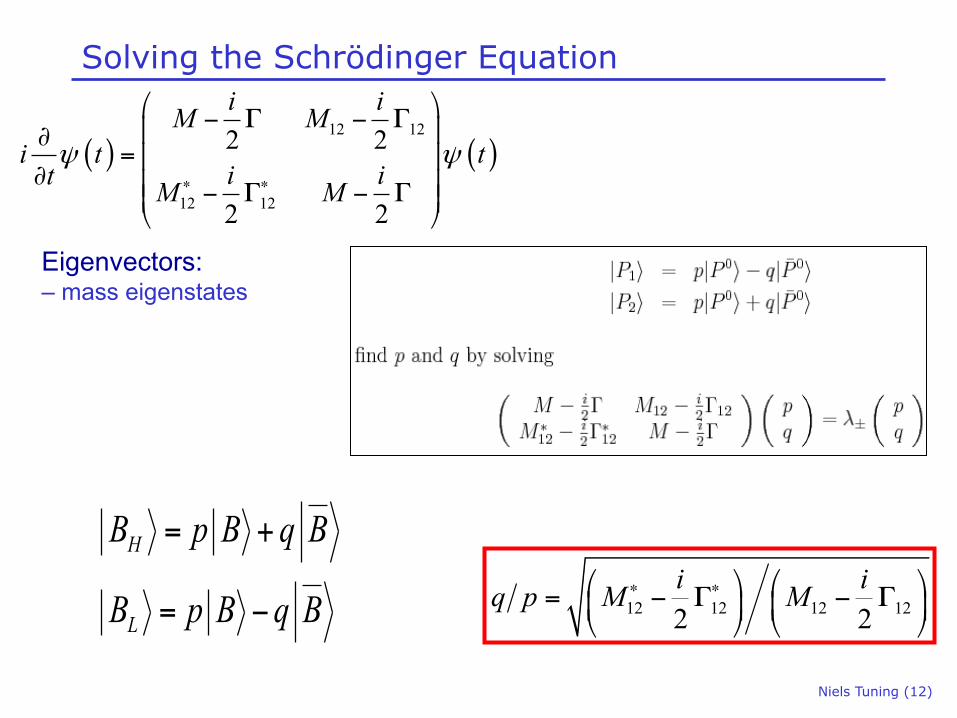
Solving the Schrödinger Equation

( ) ( )12 12

12 12

2 2

2 2

i iM Mi t t

i it M Mψ ψ

∗ ∗

⎛ ⎞− Γ − Γ⎜ ⎟∂= ⎜ ⎟

∂ ⎜ ⎟− Γ − Γ⎜ ⎟⎝ ⎠

Eigenvectors: –  mass eigenstates

H

L

B p B q B

B p B q B

= +

= − 12 12 12 122 2i iq p M M∗ ∗⎛ ⎞ ⎛ ⎞= − Γ − Γ⎜ ⎟ ⎜ ⎟

⎝ ⎠ ⎝ ⎠

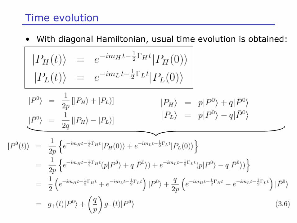
Time evolution

Niels Tuning (13)

•  With diagonal Hamiltonian, usual time evolution is obtained:

Niels Tuning (14)

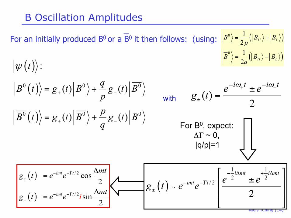
B Oscillation Amplitudes

( )

( )

( )

0 0 0

0 0 0

:

( ) ( )

( ) ( )

t

qB t g t B g t BppB t g t B g t Bq

ψ

+ −

+ −

= +

= +

( )2

i t i te eg tω ω+ −

±

− −±=

For B0, expect: ΔΓ ~ 0, |q/p|=1

( )1 12 2

/ 2

2

i mt i mtimt t e eg t e e

− Δ + Δ

− −Γ±

⎡ ⎤±⎢ ⎥

⎢ ⎥⎢ ⎥⎣ ⎦

;( )

( )

/ 2

/ 2

cos2

sin2

imt t

imt t

mtg t e e

mtg it e e

− −Γ+

− −Γ−

Δ=

Δ=

( )

( )

0

0

1212

H L

H L

B B Bp

B B Bq

= +

= −

For an initially produced B0 or a B0 it then follows: (using:

with

~

Niels Tuning (15)

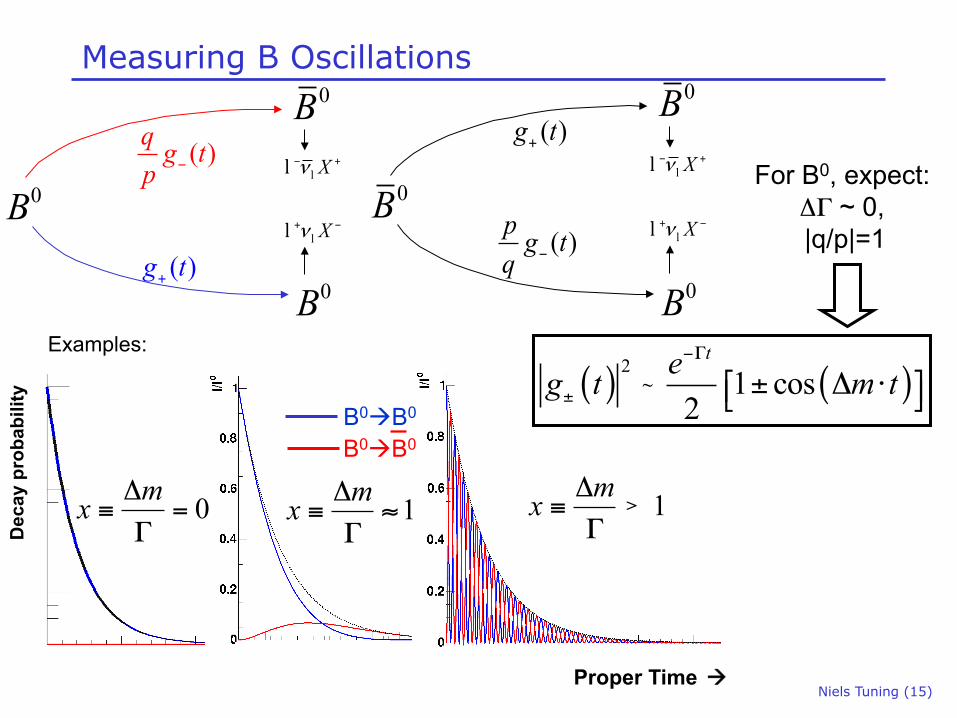
Measuring B Oscillations

( )g t+

( )q g tp −

0B

0B

0B

Xν+ −ll

Xν− +ll

Dec

ay p

roba

bilit

y

( )g t+

( )p g tq −

0B

0B

0B

Xν+ −ll

Xν− +ll

B0àB0

B0àB0

Proper Time à

0mx Δ≡ =

Γ1mx Δ

≡Γ?1mx Δ

≡ ≈Γ

For B0, expect: ΔΓ ~ 0, |q/p|=1

( ) ( )2

1 cos2

teg t m t−Γ

± ± Δ ⋅⎡ ⎤⎣ ⎦;Examples:

~

>

Niels Tuning (16)

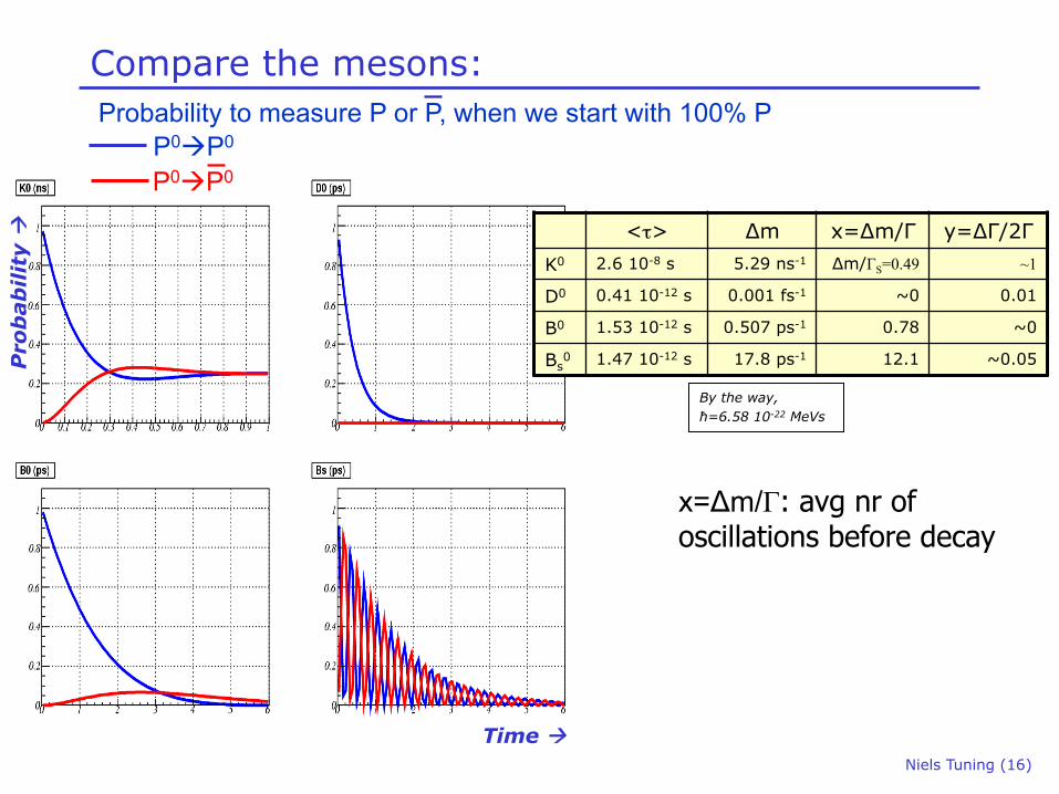
Compare the mesons:

P0àP0

P0àP0

Probability to measure P or P, when we start with 100% P

Time à

Pro

bab

ility

à

<τ> Δm x=Δm/Γ y=ΔΓ/2Γ K0 2.6 10-8 s 5.29 ns-1 Δm/ΓS=0.49 ~1

D0 0.41 10-12 s 0.001 fs-1 ~0 0.01

B0 1.53 10-12 s 0.507 ps-1 0.78 ~0

Bs0 1.47 10-12 s 17.8 ps-1 12.1 ~0.05

By the way, ħ=6.58 10-22 MeVs

x=Δm/Γ: avg nr of oscillations before decay

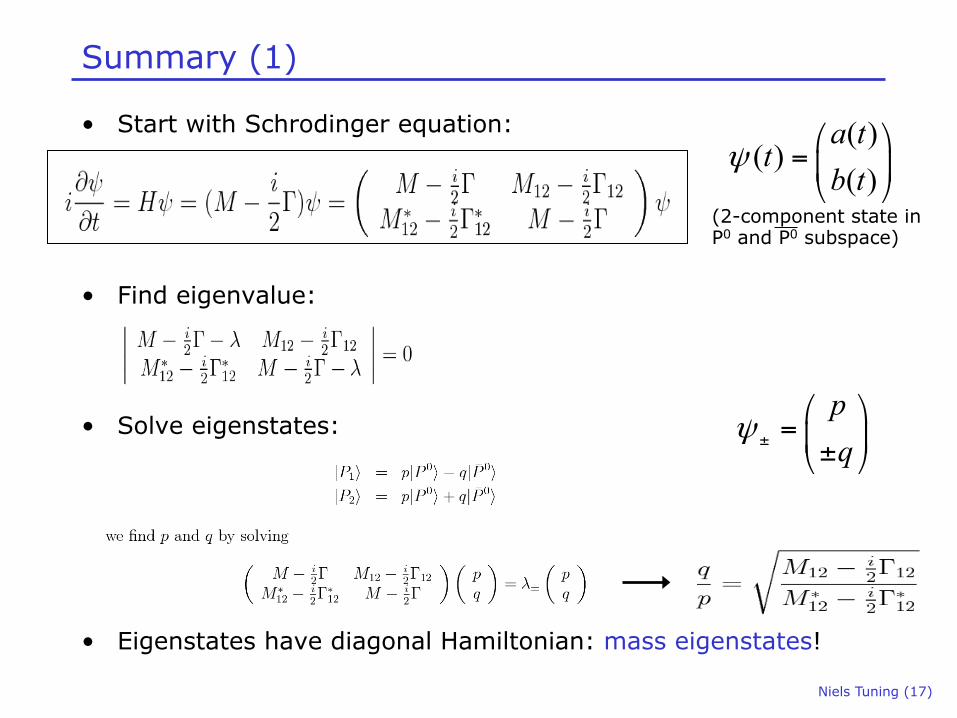
Summary (1)

•  Start with Schrodinger equation:

•  Find eigenvalue:

•  Solve eigenstates:

•  Eigenstates have diagonal Hamiltonian: mass eigenstates!

( )( )

( )a t

tb t

ψ⎛ ⎞

= ⎜ ⎟⎝ ⎠

(2-component state in P0 and P0 subspace)

pq

ψ ±

⎛ ⎞= ⎜ ⎟±⎝ ⎠

Niels Tuning (17)

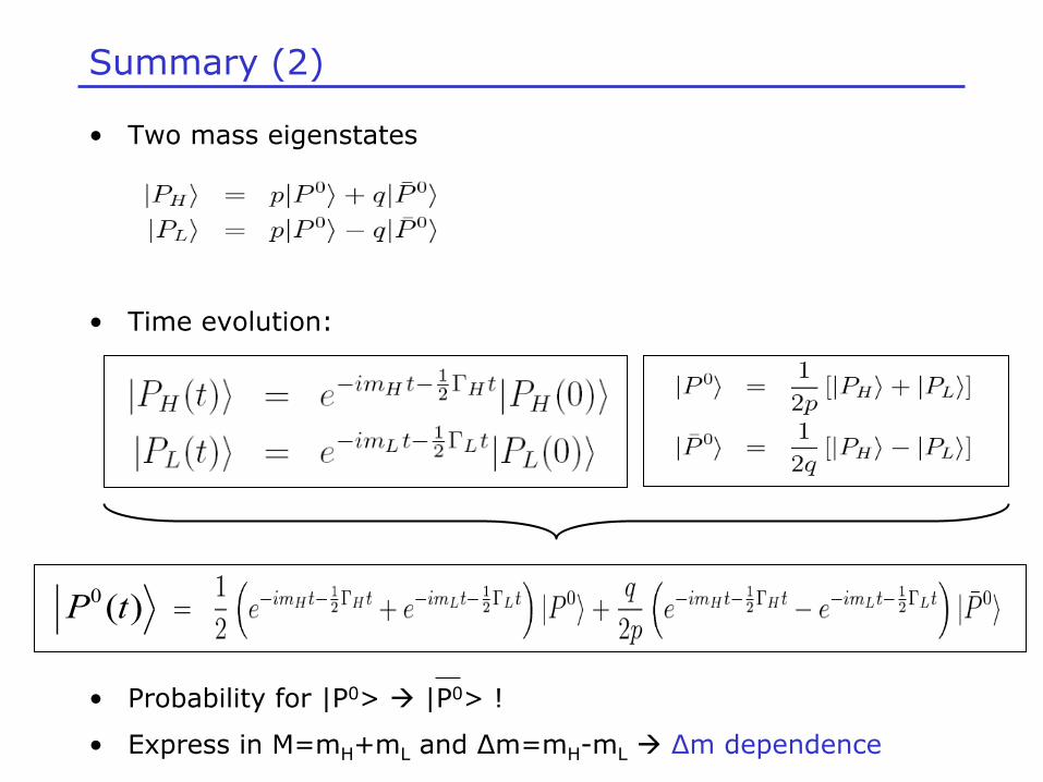
Summary (2)

•  Two mass eigenstates

•  Time evolution:

•  Probability for |P0> à |P0> !

•  Express in M=mH+mL and Δm=mH-mL à Δm dependence

0 ( )P t

Niels Tuning (19)

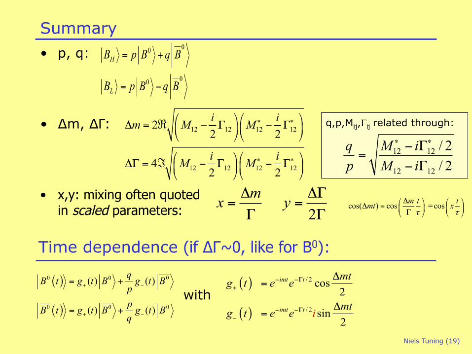
Summary 00

00

H

L

B p B q B

B p B q B

= +

= −

•  p, q:

•  Δm, ΔΓ:

•  x,y: mixing often quoted in scaled parameters:

12 12 12 1222 2i im M M ∗ ∗⎛ ⎞⎛ ⎞Δ = ℜ − Γ − Γ⎜ ⎟⎜ ⎟

⎝ ⎠⎝ ⎠

12 12 12 1242 2i iM M ∗ ∗⎛ ⎞⎛ ⎞ΔΓ = ℑ − Γ − Γ⎜ ⎟⎜ ⎟

⎝ ⎠⎝ ⎠

( )

( )

0 0 0

0 0 0

( ) ( )

( ) ( )

qB t g t B g t BppB t g t B g t Bq

+ −

+ −

= +

= +

12 12

12 12

/ 2/ 2

M iqp M i

∗ ∗− Γ=

− Γ

q,p,Mij,Γij related through:

( )

( )

/ 2

/ 2

cos2

sin2

imt t

imt t

mtg t e e

mtg it e e

− −Γ+

− −Γ−

Δ=

Δ=

with

Time dependence (if ΔΓ~0, like for B0):

2

mx yΔ ΔΓ= =Γ Γ

cos( ) cos = cosm t tmt xτ τ

Δ⎛ ⎞ ⎛ ⎞Δ = ⎜ ⎟ ⎜ ⎟Γ⎝ ⎠ ⎝ ⎠

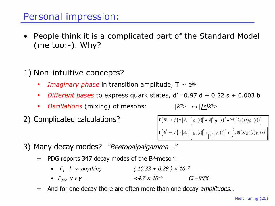
Personal impression:

•  People think it is a complicated part of the Standard Model (me too:-). Why?

1) Non-intuitive concepts? §  Imaginary phase in transition amplitude, T ~ eiφ

§  Different bases to express quark states, d’=0.97 d + 0.22 s + 0.003 b

§  Oscillations (mixing) of mesons: |K0> ↔ |�K0>

2)  Complicated calculations?

3)  Many decay modes? “Beetopaipaigamma…”

–  PDG reports 347 decay modes of the B0-meson:

•  Γ1 l+ νl anything ( 10.33 ± 0.28 ) × 10−2

•  Γ347 ν ν γ <4.7 × 10−5 CL=90%

–  And for one decay there are often more than one decay amplitudes… Niels Tuning (20)

( ) ( ) ( ) ( ) ( )( )

( ) ( ) ( ) ( ) ( )( )

2 2 220

20 2 2

2 2

2

1 2

f

f

B f A g t g t g t g t

B f A g t g t g t g t

λ λ

λλ λ

∗+ − + −

∗ ∗+ − + −

⎡ ⎤Γ → ∝ + + ℜ⎣ ⎦

⎡ ⎤Γ → ∝ + + ℜ⎢ ⎥

⎢ ⎥⎣ ⎦

Niels Tuning (21)

Describing Mixing

M12 describes B0 ↔ B0 via off-shell states, e.g. the weak box diagram

Γ12 describes B0↔f↔B0 via on-shell states, eg. f=π+π-

Time evolution of B0 and�B0 can be described by an effective Hamiltonian:

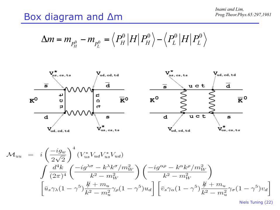
Box diagram and Δm

0 00 0 0 0

H LH H L LP P

m m m P H P P H PΔ = − = −

Niels Tuning (22)

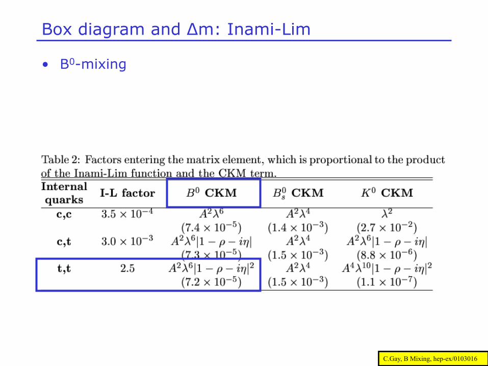
Inami and Lim, Prog.Theor.Phys.65:297,1981

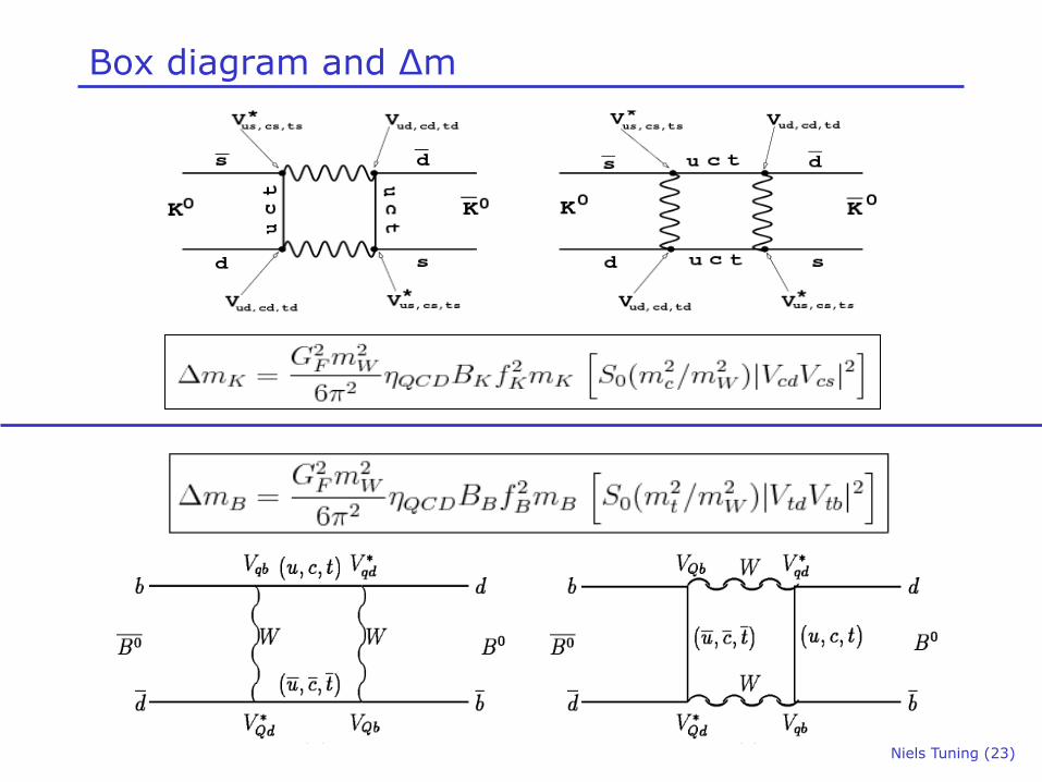
Box diagram and Δm

Niels Tuning (23)

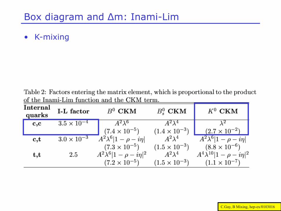
Box diagram and Δm: Inami-Lim

C.Gay, B Mixing, hep-ex/0103016

•  K-mixing

Box diagram and Δm: Inami-Lim

C.Gay, B Mixing, hep-ex/0103016

•  B0-mixing

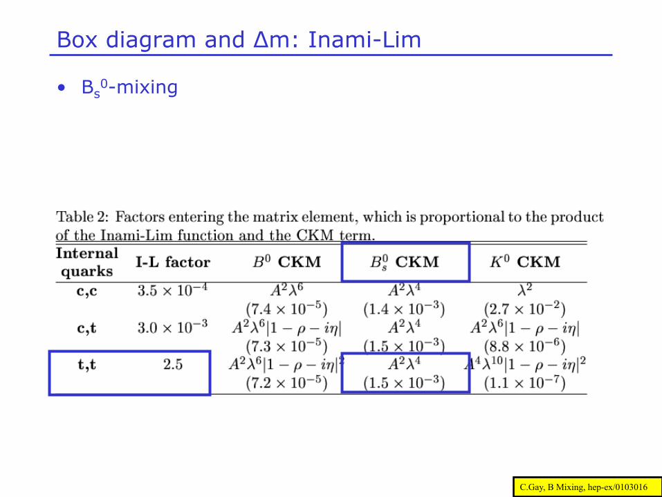
Box diagram and Δm: Inami-Lim

C.Gay, B Mixing, hep-ex/0103016

•  Bs0-mixing

Next: measurements of oscillations

1.  B0 mixing: Ø  1987: Argus, first

Ø  2001: Babar/Belle, precise

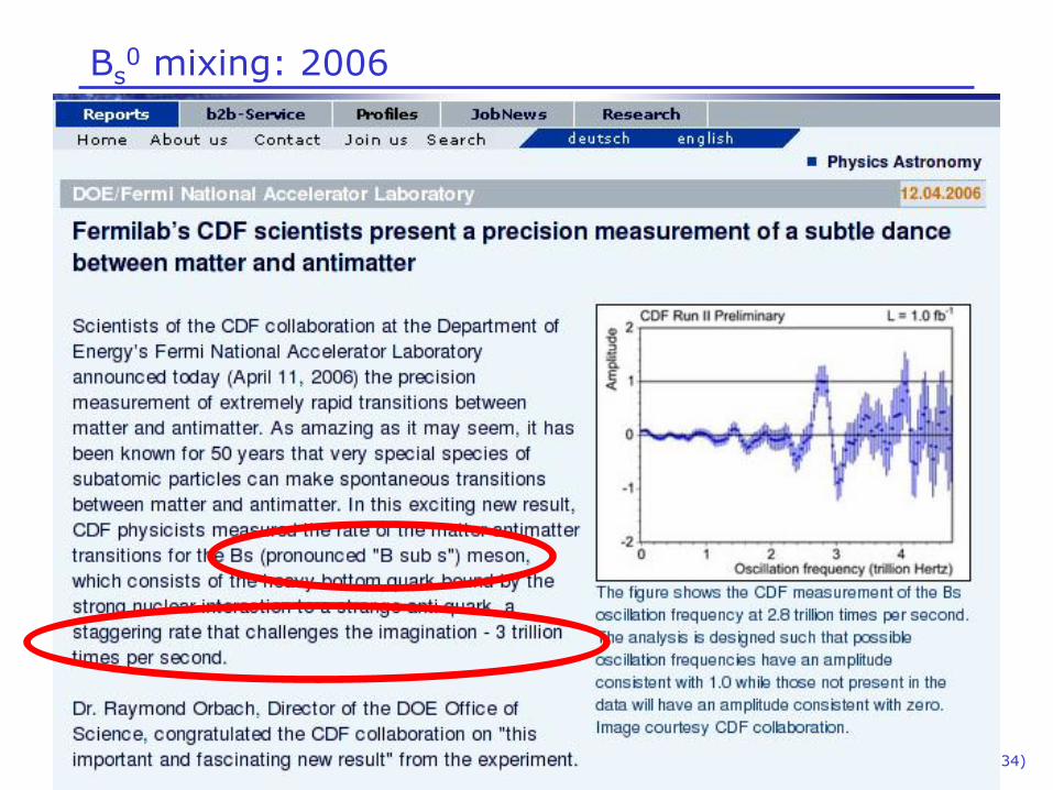
2.  Bs0 mixing:

Ø  2006: CDF: first

Ø  2010: D0: anomalous ??

Niels Tuning (27)

B0 mixing

Niels Tuning (28)

Niels Tuning (29)

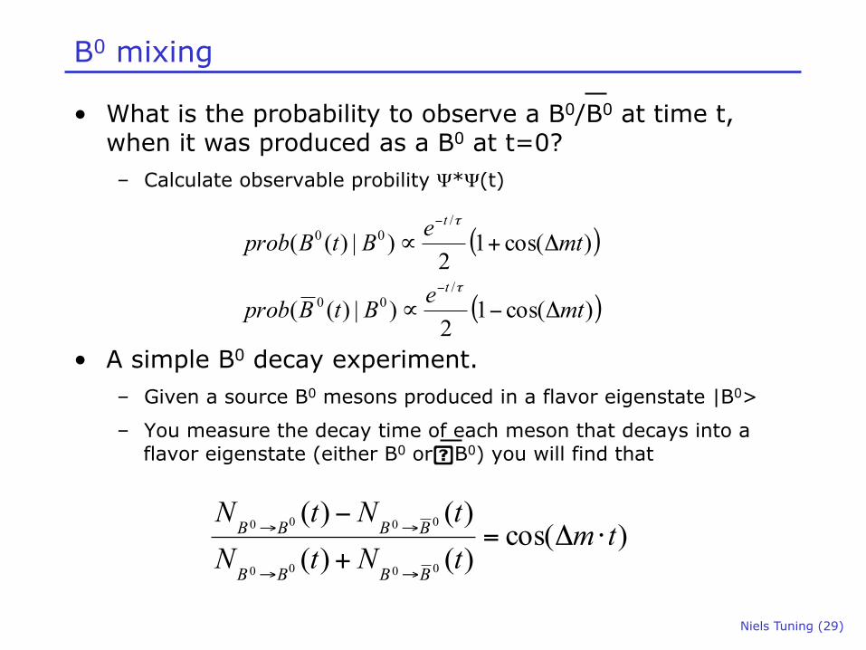
B0 mixing

•  What is the probability to observe a B0/B0 at time t, when it was produced as a B0 at t=0? –  Calculate observable probility Ψ*Ψ(t)

•  A simple B0 decay experiment. –  Given a source B0 mesons produced in a flavor eigenstate |B0>

–  You measure the decay time of each meson that decays into a flavor eigenstate (either B0 or�B0) you will find that

( )

( ))cos(12

)|)((

)cos(12

)|)((

/00

/00

mteBtBprob

mteBtBprob

t

t

Δ−∝

Δ+∝

−

−

τ

τ

)cos()()()()(

0000

0000 tmtNtNtNtN

BBBB

BBBB ⋅Δ=+

−

→→

→→

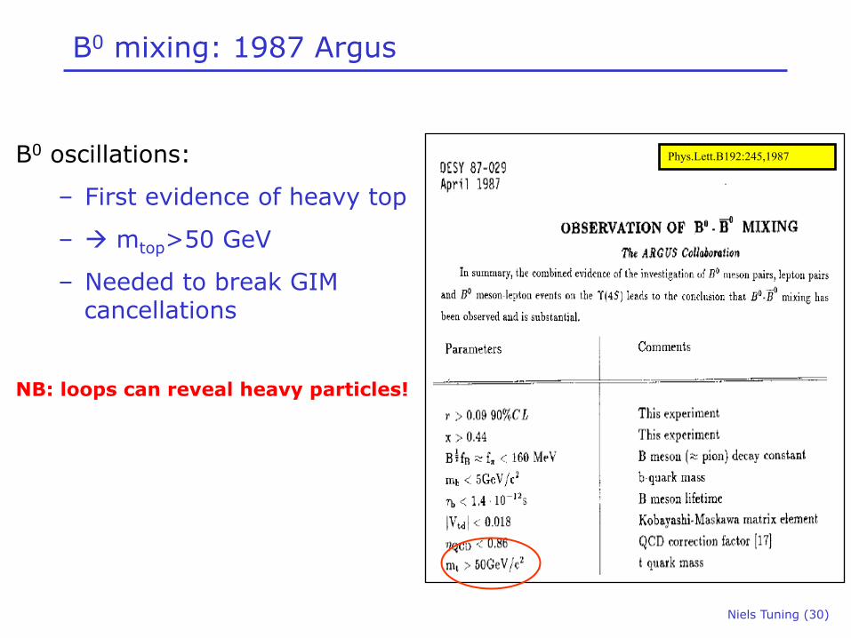
B0 oscillations:

–  First evidence of heavy top

–  à mtop>50 GeV

–  Needed to break GIM cancellations

NB: loops can reveal heavy particles!

B0 mixing: 1987 Argus

Phys.Lett.B192:245,1987

Niels Tuning (30)

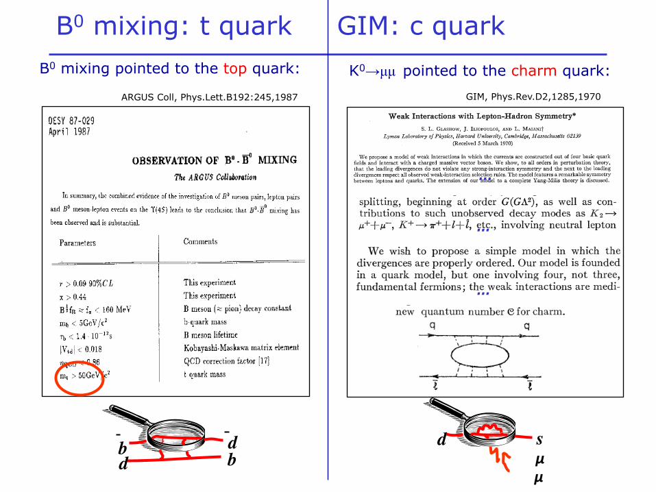
B0 mixing pointed to the top quark:

B0 mixing: t quark GIM: c quark

ARGUS Coll, Phys.Lett.B192:245,1987

b d

d b

d s

μμ

K0→µµ pointed to the charm quark: GIM, Phys.Rev.D2,1285,1970

…

…

…

Niels Tuning (32)

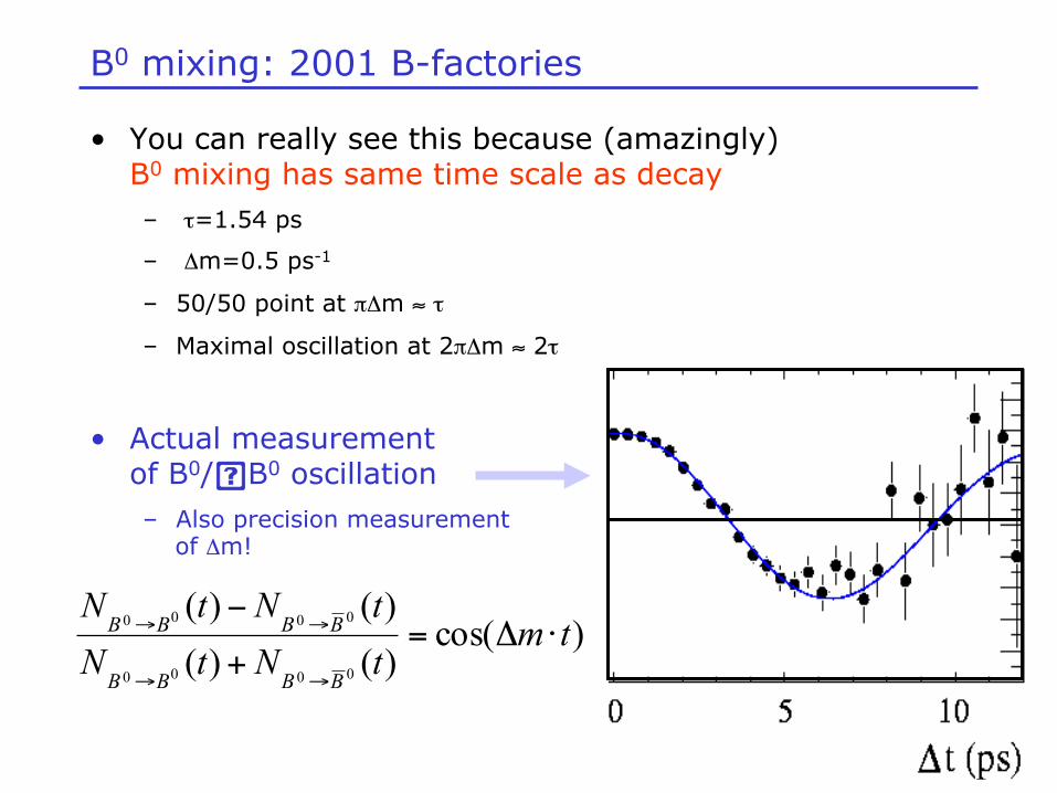
B0 mixing: 2001 B-factories

•  You can really see this because (amazingly) B0 mixing has same time scale as decay –  τ=1.54 ps

–  Δm=0.5 ps-1

–  50/50 point at πΔm ≈ τ

–  Maximal oscillation at 2πΔm ≈ 2τ

•  Actual measurement of B0/�B0 oscillation –  Also precision measurement

of Δm!

)cos()()()()(

0000

0000 tmtNtNtNtN

BBBB

BBBB ⋅Δ=+

−

→→

→→

Bs0 mixing

Niels Tuning (33)

Niels Tuning (34)

Bs0 mixing: 2006

Niels Tuning (35)

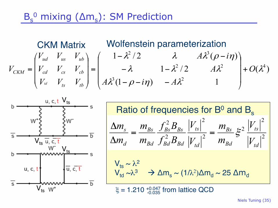
Bs0 mixing (Δms): SM Prediction

)(1)1(

2/1)(2/1

4

23

22

32

λ

ληρλ

λλλ

ηρλλλ

OAiA

AiA

VVVVVVVVV

V

tbts

cbcscd

ubusud

CKM

td

+⎟⎟⎟

⎠

⎞

⎜⎜⎜

⎝

⎛

−−−

−−

−−

=⎟⎟⎟

⎠

⎞

⎜⎜⎜

⎝

⎛

=

Vts

Vts

Vts

Vts

CKM Matrix Wolfenstein parameterization

2

22

2

2

2

2

td

ts

Bd

Bs

td

ts

BdBd

BsBs

Bd

Bs

d

s

VV

mm

VV

BfBf

mm

mm

ξ==Δ

Δ

Ratio of frequencies for B0 and Bs

ξ = 1.210 +0.047 from lattice QCD-0.035

Vts ~ λ2

Vtd ~λ3 à Δms ~ (1/λ2)Δmd ~ 25 Δmd

Niels Tuning (36)

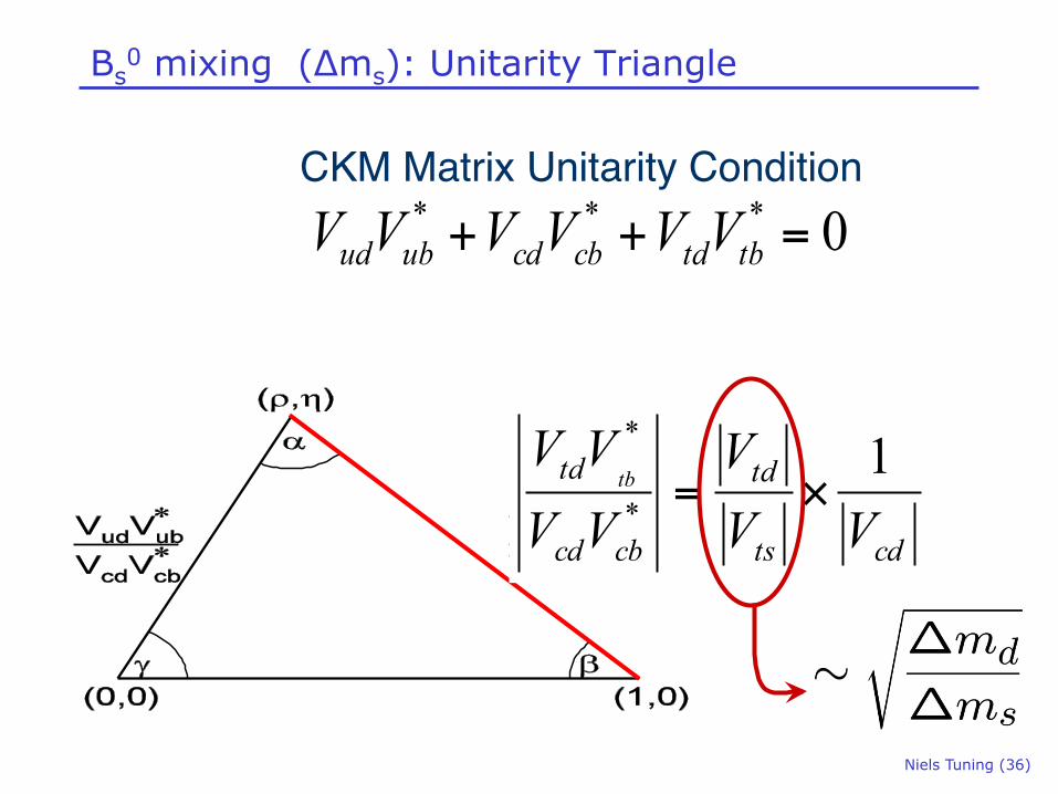
Bs0 mixing (Δms): Unitarity Triangle

0*** =++ tbtdcbcdubud VVVVVVCKM Matrix Unitarity Condition

cdts

td

cbcd

td

VVV

VVVV

tb 1*

*

×=

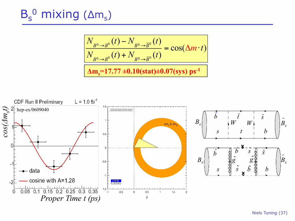
Niels Tuning (37)

Bs0 mixing (Δms)

0 00 0

0 00 0

( ) ( )cos( )

( ) ( )B B B B

B B B B

N t N tt

N t N tm→ →

→ →+

Δ−

= ⋅

Δms=17.77 ±0.10(stat)±0.07(sys) ps-1

cos

(Δm

st)

Proper Time t (ps)

hep-ex/0609040

Bs b

b

s

s t

t W W Bs

g̃ Bs Bs

b

s

s

b

x

x

b̃

b̃

s ̃

s ̃

g̃

- - - -

- - -

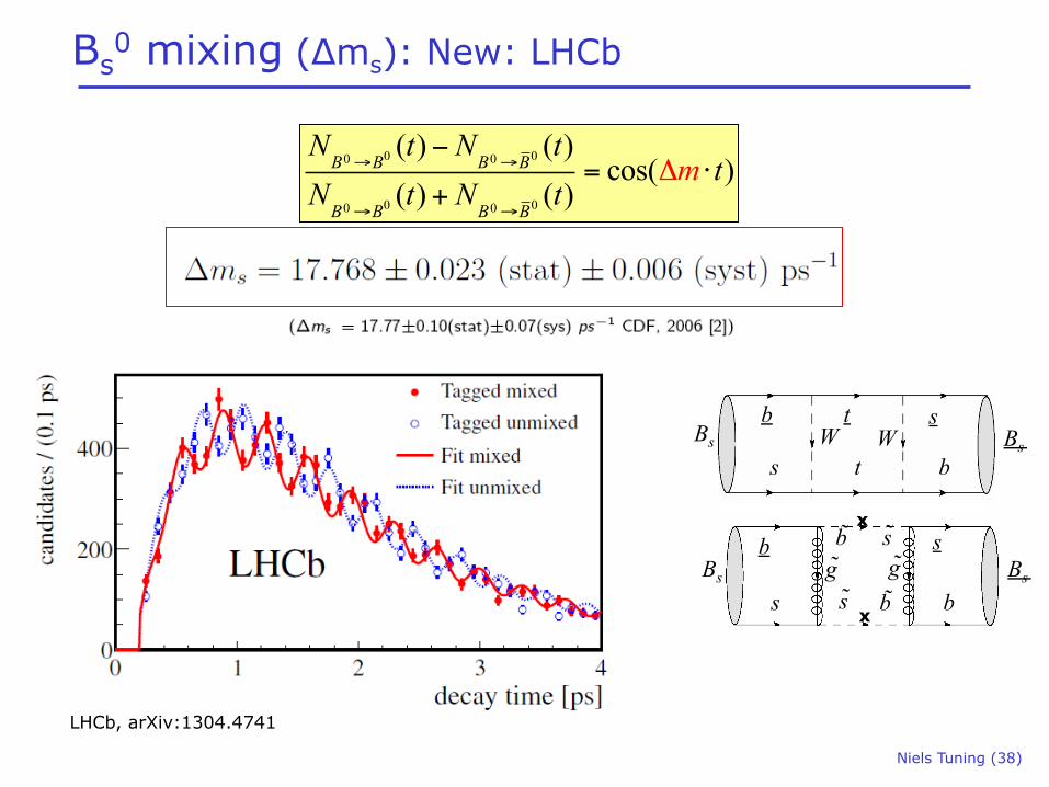
Niels Tuning (38)

Bs0 mixing (Δms): New: LHCb

0 00 0

0 00 0

( ) ( )cos( )

( ) ( )B B B B

B B B B

N t N tt

N t N tm→ →

→ →+

Δ−

= ⋅

Bs b

b

s

s t

t W W Bs

g̃ Bs Bs

b

s

s

b

x

x

b̃

b̃

s ̃

s ̃

g̃

LHCb, arXiv:1304.4741

Niels Tuning (39)

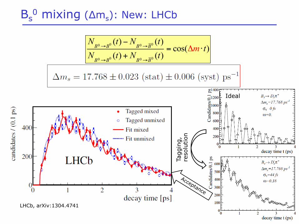
Bs0 mixing (Δms): New: LHCb

0 00 0

0 00 0

( ) ( )cos( )

( ) ( )B B B B

B B B B

N t N tt

N t N tm→ →

→ →+

Δ−

= ⋅

LHCb, arXiv:1304.4741

Ideal

Tagg

ing,

re

solu

tion

Niels Tuning (40)

Mixing à CP violation?

•  NB: Just mixing is not necessarily CP violation!

•  However, by studying certain decays with and without mixing, CP violation is observed

•  Next: Measuring CP violation… Finally

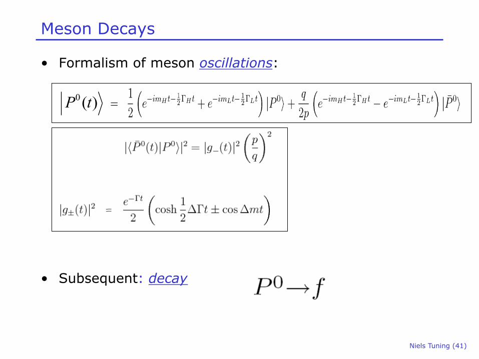
Meson Decays

•  Formalism of meson oscillations:

•  Subsequent: decay

0 ( )P t

Niels Tuning (41)

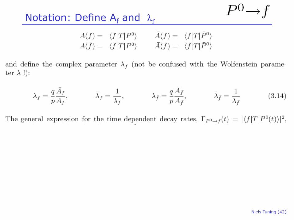
Notation: Define Af and λf

Niels Tuning (42)

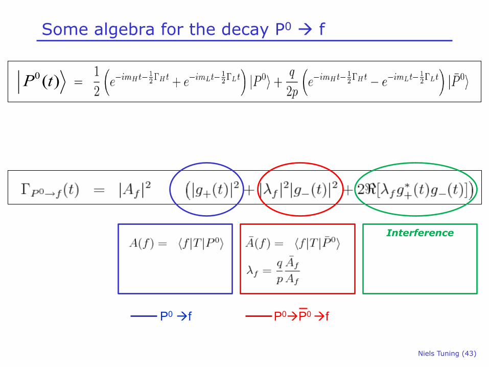
Some algebra for the decay P0 à f

0 ( )P t

Interference

P0 àf P0àP0 àf

Niels Tuning (43)

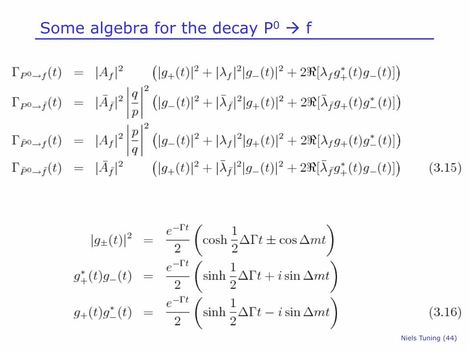
Some algebra for the decay P0 à f

Niels Tuning (44)

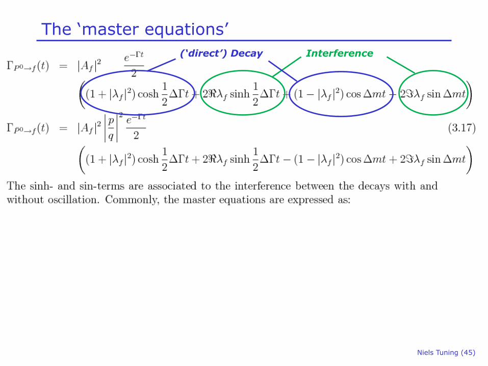
The ‘master equations’ Interference (‘direct’) Decay

Niels Tuning (45)

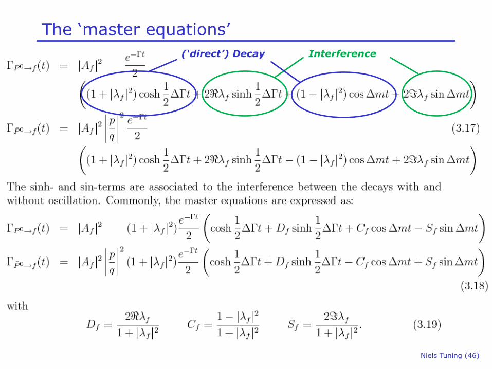
The ‘master equations’ Interference (‘direct’) Decay

Niels Tuning (46)

Classification of CP Violating effects

1.  CP violation in decay

2.  CP violation in mixing

3.  CP violation in interference

Niels Tuning (47)

What’s the time?

Niels Tuning (48)