1

Seasonal variation of microzooplankton (20 – 200μm) and its possible implications on the vertical carbon flux in the western Bay of Bengal

* 1 R. Jyothibabu, 1 N. V. Madhu, 2 P. A. Maheswaran, 1 K. V. Jayalakshmy, 1 K. K. C. Nair and 1 C. T. Achuthankutty

1 National Institute of Oceanography, Regional Centre, Kochi - 682018, India 2 Naval Physical Oceanography Laboratory, Kochi - 682021, India

Abstract

Stratification (throughout the year) and low solar radiation (during monsoon periods) have caused

low chlorophyll a and primary production (seasonal av. 13 – 18 mg m-2 and 220 – 280 mg C m-2

d-1 respectively) in the western Bay of Bengal (BoB). The microzooplankton (MZP) community

of BoB was numerically dominated by heterotrophic dinoflagellates (HDS) followed by ciliates

(CTS). The highest MZP abundance (av. 665 � 226 x 104 m-2), biomass (av. 260 � 145 mg C m-2)

and species diversity (Shannon weaver index 2.8 � 0.42 for CTS and 2.6 � 0.35 for HDS) have

occurred during the spring intermonsoon (SIM). This might be due to high abundance of smaller

phytoplankton in the western BoB during SIM as a consequence of intense stratification and

nitrate limitation (nitracline at 60m depth). The strong stratification during SIM was biologically

evidenced by intense blooms of Trichodesmium erythraeum and frequent Synechococcus – HDS

associations. The high abundance of smaller phytoplankton favors microbial food webs where

photosynthetic carbon is channeled to higher trophic levels through MZP. This causes less

efficient transfer of primary organic carbon to higher trophic levels than through the traditional

food web. The microbial food web dominant in the western BoB during SIM might be responsible

for the lowest mesozooplankton biomass observed (av. 223 mg C m-2). The long residence time of

the organic carbon in the surface waters due to the active herbivorous pathways of the microbial

food web could be a causative factor for the low vertical flux of biogenic carbon during SIM.

Key words: microzooplankton, food web, chlorophyll a, primary production, stratification, species diversity, synechococcus, Bay of Bengal, Indian Ocean

® 1 Corresponding author, E mail – rjyothi1@yahoo.co.in

2

1. Introduction

Microzooplankton (20 – 200 �m) play a significant role in energy transfer through marine

pelagic food web and hence their ecology and dynamics receive attention worldwide (Beers &

Stewart, 1971; Godhantaraman & Uye, 2001; Quevedo et al., 2003). Due to small body size,

microzooplankton (MZP) have higher weight specific physiological rates such as feeding,

respiration, excretion and growth than large zooplankton (Verity, 1985; Fenchel, 1987). They

efficiently feed on pico and nanoplankton that are generally unutilized by large zooplankton

(Marshall, 1973; Nival & Nival, 1976) and act as a significant food source for a variety of

invertebrate and vertebrate predators (Robertson, 1983; Stoecker & Capuzzo, 1990; Fukami et al.,

1999).

The Bay of Bengal (BoB), the eastern part of the northern Indian Ocean, is landlocked in

the north by the Asian continent. All the major rivers of India (Krishna, Kavery, Godavari,

Mahanadi, Brahmaputra, Ganges) flow into the BoB. During monsoon periods (June to September

– Summer monsoon, November to February – Winter monsoon), large volume of freshwater and

suspended sediments reaches in to the BoB through these rivers (1.6 x 10 12 m3 of fresh water

influx reaches BoB per year: Subramanian, 1993). The resulting low salinity plays a major role in

various exchange processes between the atmosphere, surface and deep waters that eventually

affect the biological and biochemical processes (Ittekot et al., 1991; Prasannakumar et al., 2002).

The BoB is conventionally referred as an oligotrophic system where nitrate depletion in

the surface waters (intense during spring intermonsoon period) and shortage of solar radiation

(during monsoon periods) restrict the phytoplankton growth (Gomes et al., 2000; Prasannakumar

et al., 2002; Madhupratap et al., 2003; Madhu et al., 2006). Due to the lack of solar radiation

during monsoon periods, the phytoplankton community does not efficiently utilize the high

amount of nutrients present in the inshore regions. This unutilized river - borne nutrients would

eventually be lost into the ocean depths along with settling particles (Sengupta et al., 1977;

Madhupratap et al., 2003). Another important factor causing oligotrophy in the western BoB is the

low saline surface layer that inhibits the advection of nutrients from the subsurface

(Prasannakumar et al., 2002). Although BoB is known to be oligotrophic, the vertical fluxes of

biogenic carbon are comparable in magnitude with the highly productive Arabian Sea

(northwestern part of the Indian Ocean).This is possibly due to the aggregation of biogenic carbon

with mineral particles of the river runoff which increase the speed of settling (Ittekot et al., 1991).

Another possible mechanism suggested for the high vertical organic flux in the BoB is the

3

occurrence of mesoscale eddies capable of enhancing biological production (Prasannakumar et al.,

2004).

Information on the plankton community of the BoB is very limited (Achuthankutty et al.,

1980; Nair et al., 1981; Rakhesh et al., 2006). The MZP community of the open waters of BoB

has not received an earlier study. Therefore, information available on MZP from the east coat of

India is confined to the tintinnids inhabiting in the near shore and estuarine waters

(Krishnamurthy & Naidu, 1977; Godhantaraman & Krishnamurthy, 1997; Mishra & Panigrahy,

1999; Godhantaraman, 2001; Gauns et al., 2005). Although the plankton food webs in stratified

and mixed marine waters and its consequences on the biogeochemistry of ecosystems have been

recognized (Azam et al., 1983; Cushing, 1989), there is a scarcity of such information from the

western BoB. The surface layer stratification and oligotrophy of BoB give a general impression

that MZP stock in the system could play an important role in transferring primary organic carbon

to higher trophic levels. Therefore, the present study was planned (a) to generate baseline

information on the abundance, biomass of microzooplankton in the BoB (b) to understand the

influence of the seasonally varying environment on MZP in the BoB and (c) to infer the possible

role of MZP in the seasonally varying vertical biogenic flux in the BoB.

2. Methods

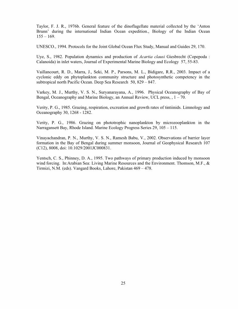
The various sampling locations in the western BOB are shown in Figure 1. Samplings

were carried out onboard FORV Sagar Sampada during March 2001 (spring intermonsoon -

SIM), December 2001 (winter monsoon - WM) and July 2002 (summer monsoon - SM).

Altogether, 28 stations were sampled in 6 transects (along 11, 13, 15, 17, 19 and 20.5°N) for

physical parameters such as salinity and temperature. Out of the 28 stations, 17 (A 1 – A 17) were

sampled for chemical (nitrate and dissolved oxygen) and biological parameters (chlorophyll a,

primary production, MZP and mesozooplankton). The stations at each transect were categorized

into inshore (station near to the coast), offshore (station at the center) and oceanic (station farthest

from the coast). To maintain the same depth of sampling and to address the same extent of the

upper water column in all the stations, the inshore stations were fixed in ~200m depth zones.

2.1. Temperature, salinity and transparency

A bucket thermometer was used to measure the Sea Surface Temperature (SST). Sea

Surface Salinity (SSS) was measured by an autosal (Guidline 8400A) calibrated with the standard

4

seawater (IAPO, Charlottenlund slot, Denmark). The vertical profile of temperature and salinity

of each station was collected from the respective sensors of the Conductivity Temperature Depth

Profiler (Seabird Electronics Sea sat, SBE 911 Plus, USA) and the data were used for

understanding the general hydrography of the region. Due to the high fresh water influx in the

study area, the Mixed Layer Depth (MLD) was taken as the depth at which the sigma – t values is

greater than the surface value by 0.2 (Prasannakumar et al., 2004). Secchi disc was operated in the

inshore and oceanic stations for measuring the transparency and thereby to assess the variability

of the euphotic column. Three times of the secchi depth was considered as the approximate lower

limit of the euphotic column (Prickard & Emery, 1982).

2.2. Dissolved oxygen and nitrate

The Go Flow bottles mounted on a CTD rosette were used to collect water samples from 9

discrete depths (0.5m, 10m, 20m, 30m, 50m, 75m, 100m, 120 and 150m) for measuring dissolved

oxygen and nitrate. Water samples for dissolved oxygen were carefully collected into glass bottles

and analyzed subsequently following Winkler’s titration method. The concentration of nitrate in

the water samples was analyzed by an autoanalyser (SKALAR, Model 51001-1) following the

principle of Grasshoff (1983).

2.3. MZP

The heterotrophic organisms with a body size between 20 – 200μm were only considered

for the study. Water samples (5 – 7 liter) were collected from 8 discrete depths (0.5m, 10m, 20m,

50m, 75m, 100m, 120m and 150m) for MZP were gently prefiltered through a 200 μm bolting

silk to remove the mesozooplankton. Although the screening of samples through 200μm sieve

may disturb large and fragile MZP, this process is widely used in MZP sampling for discarding

the mesozooplankton (Froneman and McQuaid 1997; Putland, 2000; Stelfox - Widdicombe et al.,

2004). Subsequently, 3 – 8% of Acid Lugol’s Iodine was added in to these samples. These

samples were then concentrated by gravity settling and siphoning procedure. Thus the samples

were concentrated to 100 ml volume and preserved in 1 - 3% acid Lugol's solution. Prior to the

microscopic analysis, the initial sample concentrates of MZP (1litre) were allowed to settle for 2

days. Subsamples of the settled samples were taken in Sedgwick rafter counting chamber and

observed under an inverted microscope with phase contrast optics at 100 – 400x magnifications.

Although there are some conflict existing regarding the suitable fixative for MZP, the Lugol’s

iodine is regarded as the most useful one and widely used that can make minimum damage to

5

different groups of MZP community (Gifford & Caron., 2000). The organisms present in the

samples were identified and categorized in to four groups viz., heterotrophic dinoflagellates

(HDS), ciliates (CTS), sarcordines (SDS) and crustacean nauplii (CNP) based on literature. The

CTS and HDS were identified down to the species level wherever possible and the SRS and CNP

were identified down to the group level following available literature (Kofoid and Campbell,

1939; Jorgenson, 1924; Marshall, 1969; Steidinger, 1970; Subrahmanyan, 1971; Taylor, 1976 a &

b, 1987; Gopinathan & Pillai, 1975; Corliss, 1979; Maeda & Carey, 1985; Maeda, 1986; Lynn et

al., 1988). Appropriate body dimensions of the organisms were measured using a micrometer and

the cell volume was determined based on the geometric shapes. Available numerical factors were

used to calculate the organic carbon content of CTS (0.19 pgC μm-3 - Putt & Stoecker, 1989),

HDS (0.14 pgC μm-3 - Lessard, 1991), SRS (0.0026 pgC μm-3 for acantherians and 0.018 -0.18

pgC μm-3 for foramnifers- Michaels et al., 1995) and CNP (16 ngC per individual -Uye, 1982).

The abundance and biomass of MZP at different discrete depths were mathematically formulated

to address the surface layer (upper 10m water column - values at the 0.5m and 10m were

integrated) and the entire water column (values from 0.5m to 150m were integrated).

2.4. Chlorophyll a & primary production

Two litre of water samples were collected from 7 standard depths (0.5, 10, 20, 50, 75, 100

and 120 m) using Go Flo bottles. These samples were then passed through GF/F filters and the

chlorophyll a was extracted in 10 ml 90% acetone (Qualigens AR, Mumbai). The measurement of

chlorophyll a was carried out using a spectrophotometer following the procedure of Strickland &

Parsons (1972). Water samples for estimating primary productivity (2 litre) were obtained from

seven standard depths before dawn (~ at 0500 hours) and transferred to five clean Nalgene

polycarbonate bottles for the insitu 14C experiment (UNESCO, 1994). Column values of

chlorophyll a and primary production were calculated by integrating the discrete depth values up

to 120m.

2.5. Mesozooplankton

A Multiple Plankton Net (Hydro - Bios, mouth area 0.25 m2, mesh width 200 μm) with an

electronic depth sensor was operated vertically to collect mesozooplankton samples. Samples

were collected from the bottom of thermocline to the surface to get a fair representation of the

euphotic column. The zooplankton collections were carried out around the noon to avoid the

possible error on biomass due to vertical migration. Mesozooplankton biomass was measured as

6

displacement volume and then converted to organic carbon using numerical factors proposed by

Madhupratap & Haridas, 1990 (1ml displacement volume = 0.075g dry weight; 32.5% of the dry

weight represent the organic carbon content – Gauns et al., 2005).

2.6. Statistical analyses

Three-way Analysis of Variance (ANOVA) was used to study the significance of

variability of MZP between stations, between species and between depths. This analysis also

helps to see the station – species, station – depth and species - depth specificity/interaction of CTS

and HDS (Snedecor & Cochran, 1967). In representative stations Multi Dimensional Scaling

(MDS) analysis was carried out to see the species clustering/specificity at different discrete depths

using Plymouth Routine in Marine Environmental Research) (PRIMER - Clarke & Gorley, 2001).

The primary goal of the MDS is to detect meaningful underlying dimensions that allow the

researcher to explain observed similarities or dissimilarities (distances) between the investigated

objects. MDS attempts to arrange "objects" (in the present case MZP species abundance at

different depths) in a space so as to reproduce the observed similarities. As a result, we can

explain the distances in terms of dissimilarity between species occurring in different depths. In

more technical terms, it uses a function minimization algorithm that evaluates different

configurations with the goal of maximizing the goodness-of-fit (or minimizing "lack of fit").

Stress (measures of goodness of fit), the most common measure that is used to evaluate how well

(or poorly) a particular configuration reproduces the observed distance matrix (please see

http://www.statsoft.com/textbook/stmulsca.html for further details).

Diversity is a concise expression of how individuals of a community are distributed in

subsets of groups. To analyze changes in MZP community due to environmental influence,

following diversity indices were also used.

2.6.1 Species richness (Margalef, 1968)

Species richness is the number of different species in a particular area

D = (S-1)/log eN

S is the number of species and N is the total number of individuals of all the species in the sample.

2.6.2 Species evenness (Heips, 1974)

7

Species evenness is the relative abundance with which each species are represented in an area

E = e (H(S) – 1/S-1)

H (S) is the species diversity in bits of information per individual and S is the number of species

2.6.3 Species diversity (Shannon and Weaver, 1963)

The advantage of this index is that it takes into account the number of species and the

evenness of the species. The index is increased either by having more unique species, or

by having a greater species evenness.

H (S) = -� [pi (log 2 pi)]

Pi = ni /n (proportion of the sample belonging to the ith species).

3. Results

3.1. Physicochemical environment

During WM, marked latitudinal variation of SST was prevalent in the study area (26 –

29�C) with a decreasing trend towards north. The SST in the region was highest during SIM (33 –

34� C) followed by the SM (27 – 30�C) and its latitudinal variation was not prominent during

these periods (Figure 2). SSS was markedly low in localized regions along the coast during WM

and in the north during SM. SSS at station A7 (24) and A16 (25) were the lowest during WM and

in all other stations its variability was not pronounced (32 – 34) (Figure 2). During WM, MLD

was low (<15m) at station A7 and A16 compared to all other locations (18 – 50m) due to high

river influx. Similarly, during SM, at stations A13 and A17, SSS was markedly low (29 and 28)

compared to all other stations (32 – 33) due to the high river influx. A similar decrease (<10m)

was found in the MLD in these stations compared to all other stations (20 – 55m). The variation in

SSS between stations was minimum during SIM (32 –34). The MLD in the entire region was low

during SIM that varied from 8 – 25m. Among different seasons studied, the MLD was deeper

during SM (av. 40m) and WM (av. 35m) compared to SIM (av. 17m). During all the three

periods, the euphotic depth was generally decreasing towards the north and inshore stations

(Figure 3). Seasonally, the euphotic depth was highest during the SIM (av. 107m) followed by

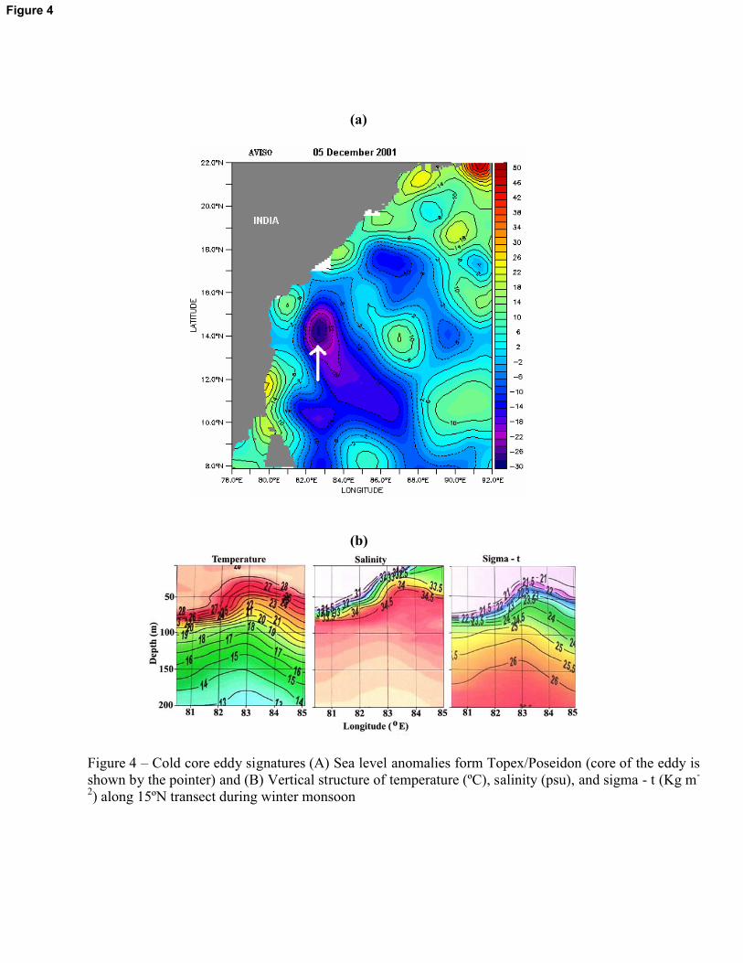
WM (75m) and SM (66m). In the vertical structures of the temperature, salinity and sigma – t, the

signature of the cold core eddy (upheaval of isolines) was evident in the subsurface layers (below

8

30m) along 15�N transect during WM (Figure 4). The core of the eddy was situated in the

offshore region between 13 and 15�N transect as evident in the satellite imagery of the sea level

anomaly (Figure 4)

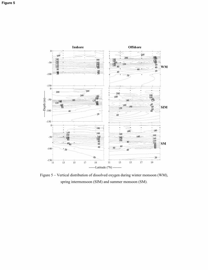
Dissolved oxygen concentration in the upper layers (upper 50m water column) was higher

during SIM compared with WM and SM periods. The decrease of dissolved oxygen concentration

during SM and WM compared to SIM was more evident in the inshore stations (Figure 5). During

SM, dissolved oxygen concentration at any specific depth in the upper 50m-water column was

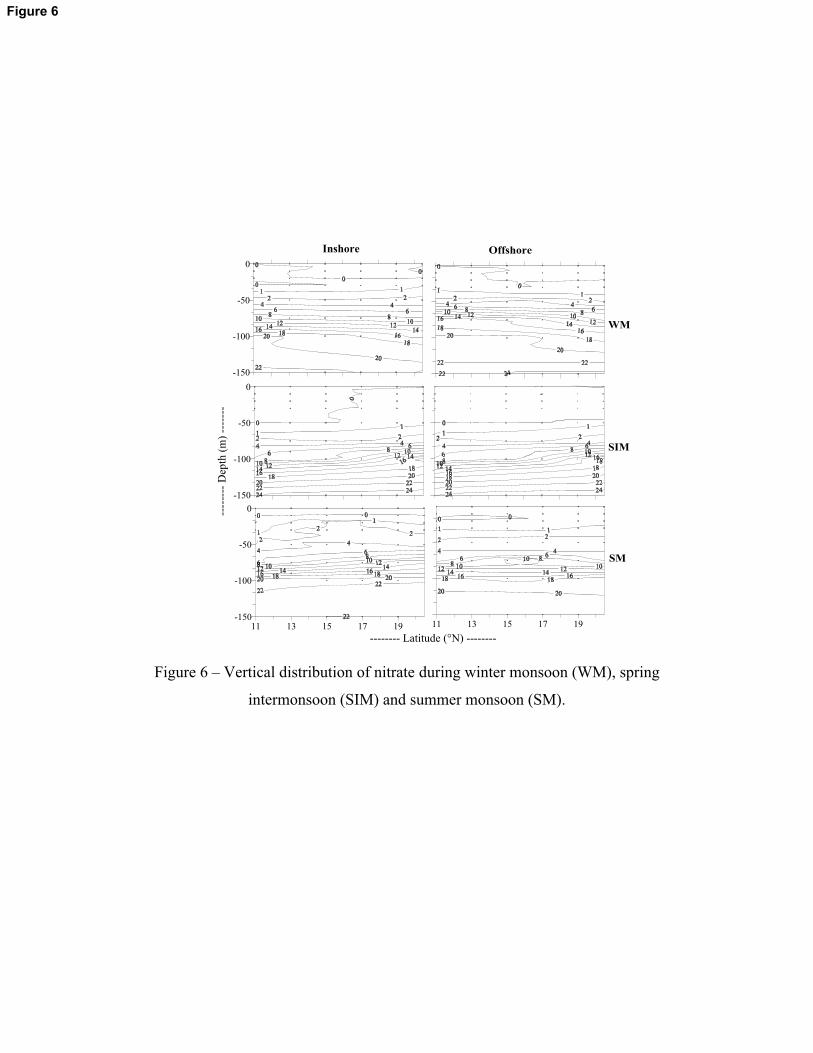
lower by 15 – 20�M less compared to SIM (Figure 5). The concentration of nitrate was below

0.5�M in the surface waters during all the three seasons (Figure 6). Depletion of nitrate in the

surface waters was severe during SIM where nitracline (1�M contour of nitrate) was at deeper

depth (60m) compared to WM (35m) and SM (30m) (Figure 6). However, during WM, 1�M of

nitrate was found at 20m of the station A15 where cold core eddy was centered.

3.2. Biological parameters

3.2.1. Chlorophyll a and primary production

Surface chlorophyll a concentration in the study area was highest during SM (av. 0.24 �

0.17 mg m-3) followed by WM (av. 0.16 � 0.23 mg m-3) and SIM (av. 0.09 � 0.07 mg m-3) (Table

1). Column chlorophyll a also showed a similar trend with high values during SM (18 � 11 mg m-

2) compared with WM (av. 14 � 3.5 mg m-2) and SIM (av. 13 � 3.6 mg m-2). Elevated chlorophyll

a (19 mg m-2) was found at station A8 during WM due to the cold core eddy. Similar to the

surface chlorophyll a, surface primary production was also highest during SM (av.11 � 13 mgC

m-3 d-1) followed by WM (5.5 � 3.1 mgC m-3 d-1) and SIM (5 � 4.4 mgC m-3 d-1) (Table 1).

However, seasonal variation in the column values of primary production was not substantial (av.

265 � 130 mgC m-2 d-1 during SM, av. 245 � 86 mgC m-2 d-1during WM and av. 242 � 96 mgC m-

2 d-1 during SIM).

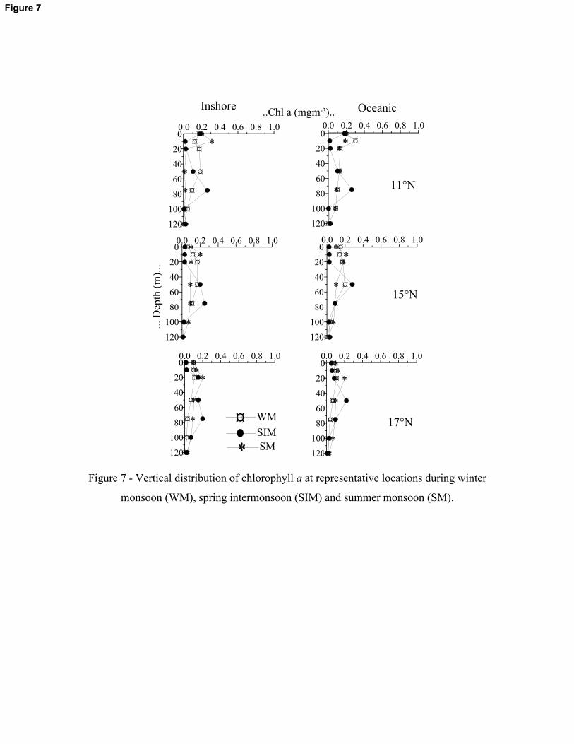
Vertical distribution of chlorophyll a showed clear seasonal trends (Figure 7). During SM

and WM periods, the high concentration of chlorophyll a was mostly with in the upper 20m-water

column. In contrast, chlorophyll a concentration was high in the subsurface layers (50 – 75m)

during SIM period (Figure 7). Three extensive blooms of Trichodesmium erythraeum

(Cyanophyta) were observed at different locations of the study area during SIM (Figure 8). These

9

blooms showed an average geographical coverage of 10 Km2 each. Two blooms were located off

Karaikkal where one was in the coastal region (11�N, 80� 60’E) and the other one in the oceanic

region (10� 58’N, 81� 50’E). The third bloom was located in the oceanic regions off south of

Kolkota (19� 44’ N, 89� 04’E).

3.2.2. MZP

3.2.2.1. Composition

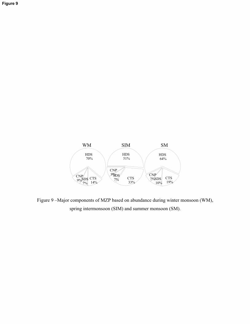
Protozoans were the dominant component of the MZP community. They consist of

heterotrophic dinoflagellates (HDS), ciliates (CTS), and sarcordines (SDS) in which the first two

groups were predominant. HDS contributed substantially to the total abundance of MZP. They

contributed to 68% of the total abundance during WM, 64% during SM and 51% during SIM

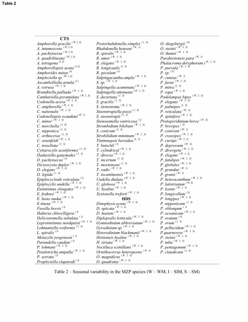
(Figure 9). Altogether 57 species of HDS were recorded in the study where the dominant genera

were Protoperidinium, Phalacroma and Ornithocercus (Table 2). CTS was the second abundant

group and their percentage contribution to the MZP community was relatively high during SIM

(33%) (Figure 9). Although CTS were numerically the second dominant group only, the generic

and species diversity were more (75 species belonging to 35 genera) than that of the HDS (57

species belonging to12 genera) (Table 2). The numerically dominant genera of CTS were

Amphorella, Codonellopsis, Eutintinnus, Salpingella and Strombidium (Table 2). Seasonal

variation was prominent in the species abundance of CTS where the highest number (78 species)

was observed during SIM followed by SM (60 species). Conversely, the HDS species abundance

showed only marginal variation seasonally (48 during SM, 47 during SIM and 50 during SM).

Among the CTS, loricates dominated quantitatively and qualitatively throughout the study with 31

genera and 72 species over aloricates with 4 genera and 6 species. SDS was the third group of

protozoans present in the MZP community and their contribution varied from 7 - 9% of the total

abundance and CNP was the metazoan component with 6 – 11% of the total abundance (Figure

9).

3.2.2.2. Abundance and biomass

Abundance of MZP in the surface waters (represent discrete depth values integrated up to

10m depth) was highest during SM (av. 175 � 38 x 104 m-2) compared with the WM and SIM (av.

49 � 10 x 104 m-2 and av. 51 � 11 x 104 m-2 respectively). However, MZP column values

(represent discrete depth values integrated up to the 150m depth) were highest during SIM (av.

665 � 226 x 104 m-2) followed by SM (av. 575 � 180 x 104 m-2) and WM (av. 350 � 109 x 104 m-

10

2) (Table 3). Biomass of MZP showed similar trends with highest surface biomass during SM

period (av. 48 � 18 mg C m-2) and highest column biomass during SIM (av. 260 � 145 mg C m-2).

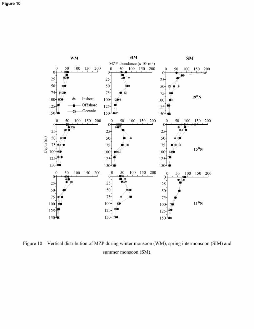
The MZP was high at shallow depth zones during WM & SM (upper 20m water column) and at

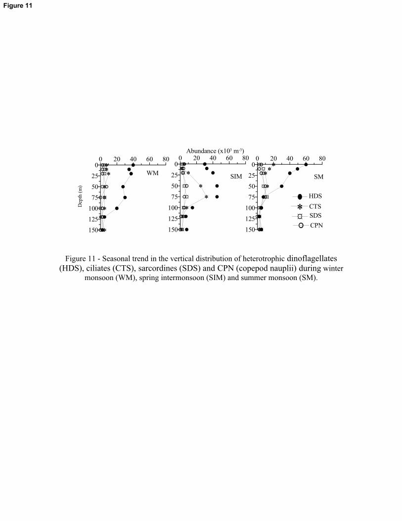
deep depth zones during SIM (50 – 75m) (Figure 10). During WM & SM, dinoflagellates were

clearly high in the surface waters compared to CTS (Figure 11). During SIM, the abundance of

dinoflagellates and CTS were high in subsurface layers, but the enhancement of the latter was

more pronounced (Figure 11). Five species of CTS viz, Salpingella acuminata, S. decurtata, S.

gracilis, S. stenosoma and Salpingacantha ampla occurred exclusively in the deeper waters,

which never appeared above 20m in the water column. These species occurred in relatively deep

zones (50 – 75m) during SIM compared to the monsoon seasons where they occurred in more

shallow depth zones (20 –50m).

Correlation between MZP biomass and phytoplankton standing stock was more during the

SIM (p<0.01, r2 = 0.38, n = 103) compared to WM (p<0.01, r2 = 0.15, n = 108) and SM (p<0.01,

r2 = 0.13, n = 94) possibly due to the seasonal variability in the qualitative composition of

phytoplankton prey and optimum temperature. To understand this more clearly, correlation

between phytoplankton biomass and the biomass of HDS and CTS were analyzed separately.

HDS were significantly correlated with phytoplankton standing stock during WM (p<0.01, r2 =

0.35, n = 103), SIM (p<0.01, r2 = 0.28, n = 103) and SM (p<0.01, r2 = 0.38, n = 103) and the

coefficient of determination was comparable in all the seasons. However, CTS were less

correlated with the phytoplankton standing stock during SM (p<0.01, r2 = 0.11, n = 103 and WM

(p<0.01, r2 = 0.21, n = 103) compared to SIM (p<0.01, r2 = 0.44, n = 103).

3.2.2.3. Species variability, interaction and diversity

The abundance of CTS and HDS between stations, between species and between depths were

significantly different (p<0.01) during all the three periods of the study (Table 4). The specificity

of HDS and CTS on stations were insignificant during all the three periods (p>0.05). CTS and

HDS showed highly significant species - depth interaction (p<0.01) during all the three seasons

except for the latter during SIM where the relation was not significant. Similarly, station - depth

interactions of CTS and HDS were highly significant during SIM (p<0.01) but found to be

insignificant during WM and SM (p>0.05) (Table 4). The preference of CTS and HDS towards

particular depths was evident in the MDS analysis also (Figure 12). The ciliates present in the 20

– 75m-depth zone showed similarity during SIM, indicating less specificity for any particular

11

depth, but during WM and SM the preference towards specific depth was more as evident from

the higher F ratio for CTS during WM (6.58) and SM (9.53) compared to SIM (4.23). Similarly,

HDS showed more specificity for depths during WM (only 10 and 20m depths showed some

similarity) and SM (only 0.5 and 10m only showed some similarity). The overall species

diversity, richness and evenness of CTS were higher during the SIM period (av. 2.7 � 0.2, 3.1 �

0.8 and 2.5 � 0.3, respectively) compared with SM (av. 2.3 � 0.3, 2.5 � 0.3 and 2.2 � 0.1,

respectively) (Table 5). Conversely, the species diversity, richness and evenness of dinoflagellates

during the SIM (av. 2.6 � 0.4, 2.1 � 0.6 and 2.3 � 0.2, respectively) were comparable in

magnitude with SM (av. 2.5 � 0.2, 2.1 � 0.3 and 2.3 � 0.1, respectively).

3.2.2.4. Association of cyanobacteria with HDS

The occurrence of cyanobacteria associated with several species of HDS was noticed

during the study. Under the epifluorescence microscope, using the blue filter, the intense orange

fluorescence of the phycoerythrin pigment of the cyanobacterial cells was distinctly visible. The

general size (~2.5�m diameter), morphology and the presence of phycoerythrin pigment suggest

that the cyanobacterial cells were Synechococcus. The association of HDS and Synechococcus in

oligotrophic marine environments was documented in several earlier studies (Taylor 1976a;

Gordon et al., 1994; Jyothibabu et al., 2006). The HDS species that showed cyanobacterial

symbionts were Ornithocercus magnificus, O. heteroporus, O. quadratus, O. steinii, O. thumii,

and Histioneis hyaline in which the first four species were predominant (Figure 13). These

dinoflagellates were restricted to the upper 50 and 75m water column during monsoon and SIM

period, respectively. The total occurrence of these dinoflagellates and the incidence of

cyanobacterial association showed clear seasonal trends. During the SIM period, out of 1747

specimens of potential dinoflagellate species observed under the microscope, 1538 (96%) had

cyanobacterial cells inside their body. During WM and SM, the frequency of incidence of

cyanobacterial associations was low in magnitude. Out of 964 specimens of potential

dinoflagellate species observed during the WM period, only 140 (15%) had cyanobacterial cells.

Similarly, among 955 specimens observed during SM, only 131 (14%) specimens had

cyanobacterial endosymbionts (see Jyothibabu et al., 2006 for more details).

3.2.3. Mesozooplankton biomass

The mesozooplankton biomass of the study area was high during WM (av. 777 � 433 mg

C m-2) and SM (av. 628 � 499 mg C m-2) compared to SIM period (av. 223 � 236 mg C m-2)

(Table 6). During WM and SM zooplankton biomass distribution showed noticeable geographical

12

variations with high biomass in the southern region of the study area during the former period and

vice versa during the latter period. However, during SIM such geographical variation was not

evident in the distribution of zooplankton biomass (Table 6). Copepods were the predominant

group in the community (seasonal av. 67 – 72%).

4. Discussion

4.1. Physicochemical environment

During WM, the intensity of atmospheric cooling in the BoB decreased towards the

northern latitudes (Hastenrath & Lamb, 1979). The occurrence of low saline waters (<30) found

localized along the coastal region during this period was due to the freshwater discharge

(Suryanarayana & Murthy, 1988). The river runoff is found to play an important role in reducing

the transparency and mixed layer depth (MLD) in the BoB (Vinayachandran et al., 2002). During

the WM period, the MLD decreased with increased freshening (causes stratification) along the

coastal and northern regions (north of 19°N). As a result, the nitracline was lowered to ~ 35m

depth, where as in the cold core eddy region it was traceable at 20m depth. The high nutrient

content brought by river seems to be restricted to the very coastal regions (Prasannakumar et al.,

2002) and therefore is not reflected in the present measurements. However, the high amount of

suspended materials brought by rivers has caused low euphotic column along the inshore regions

(av.75m).

The increased solar radiation during SIM has caused a 2- 3ºC increase in the SST and

high SSS indicated low river runoff. The poleward flowing East Indian Coastal Current probably

pushed the low saline surface waters to the offshore region resulting in low saline patches away

from the coast (Sanil Kumar et al., 1997). Thus, the warm and low saline waters in the offshore

region during SIM have amplified the stratification leading to nitrate limitation in the surface

layers (av. MLD was 20m and nitracline was 60m). The intense solar radiation and low freshwater

influx have increased the euphotic column depth (av. 108m) during SIM.

Similar to the SIM features, high SST (with minimum spatial variability) prevailed during

SM (Varkey et al., 1996) but, the SSS decreased in the northern region due to the high amount of

rainfall and river runoff (Subramanian, 1993). The high amount of suspended sediment flux from

the river and the thick cloud cover during the SM period markedly reduced the euphotic column

(av. euphotic depth was 60m). Due to the prevailing southwest monsoon winds during SM, the

MLD was relatively high in most of the study area compared to SIM &WM.

13

4.2. Biological environment

4.2.1. Phytoplankton standing stock and productivity

The low seasonal average values of phytoplankton standing stock and production in the

BoB (13 – 18 mgm-2 and 220 – 280 mg C m-2 d-1 respectively) truly represented the oligotrophy of

the system. Strong stratification prevents the upliftment of nutrients from the base of the

thermocline to the upper euphotic column as the nitracline was found below 30m depth during all

the three seasons studied. During SIM, due to intense surface layer stratification (lowest MLD),

the nitracline was at 60 m depth thereby causing intense depletion of nitrate in the surface layers.

The decrease in the euphotic column during monsoon periods was suggestive of the low

solar radiation during which, phytoplankton resides in the upper 50m water column (Gomes et al.,

2000; Madhu et al., 2006) as evidenced in the shallow chlorophyll a maxima. Nitrate was sparsely

available in the surface layer during this period compared to SIM and this might have supported

the growth of phytoplankton community in the surface layer. On the other hand, even with high

solar radiation available during SIM, high phytoplankton standing stock remained in the

subsurface layers (30-75m) due to the extreme depletion of nitrate in the surface layers (Gomes et

al., 2000).

The mesoscale eddies have been reported to promote primary production in the BoB

(Gomes et al., 2000; Prasanna Kumar et al., 2002.). The cold core eddy centered along 15�N

transect during the WM period sustained the highest chlorophyll a value of the season (16 mg m-

2). Normally, a cold core eddy produces marked enhancement of biological production through

pumping of nutrients into the upper euphotic column (McGillicudy & Robinson, 1997). During

the present WM observation, the eddy was prominent only in the subsurface waters which

probably caused moderate biological production.

4.2.2. MZP

In the western BoB, HDS was the most abundant group contributing 51 – 70% of the MZP

community in abundance during different seasons. This was in agreement with earlier

observations that HDS forms the major component of MZP in the oligotrophic marine waters of

tropical and subtropical regions (Lessard, 1991; Quevedo et al., 2003). The present study is the

first of its kind from the western BoB that gives baseline information on the qualitative

composition of the HDS community (Table 2). High quantitative occurrence of HDS (av.65%)

14

could be due to their diverse modes of feeding in diverse environmental conditions (reviews by

Gains & Elbrachter, 1987; Hansen, 1991; Lessard, 1991). The specific growth rate of HDS is less

than that of CTS, but they outnumber the latter in oligotrophic environments due to the ability to

utilize a wider range of prey through diverse modes of feeding (Jeong, 1999).

The CTS formed the second numerically dominant MZP component with 14 – 33% of the

community. This was comparable with the values obtained from the Arabian Sea (15 – 43%), off

southern California (18 – 32%) and Northern Adriatic (12 - 52%) (Gauns et al., 1996; Beers &

Stewart, 1971; Revelante & Gilmartine, 1983). However, a noticeable decrease in aloricate CTS

as reported earlier (Gauns et al., 2005) remains unexplained. The oligotrophic marine waters are

found to exhibit significant amount of aloricate ciliates compared to tintinnids (Quevedo et al.,

2003). One plausible reason for the low abundance of aloricate ciliates could be the exclusion of

organisms below 20�M due to limitations in the sampling methodology. Despite this fact, the

importance of the present study is that this forms the first detailed information on the MZP

community from the BoB.

The availability of preferential food and a warm condition are the key factors, which favor

the CTS in marine ecosystems (Heinbokel, 1978; Taniguchi & Kawakami, 1983; Verity, 1986;

Godhantaraman & Krishnamurthy, 1997). HDS increase with phytoplankton stock mostly

contributed by larger diatoms (Hansen, 1991). Thus the larger phytoplankton stock in warm

waters could be one of the reasons for the high abundance of MZP in the surface layers. During

SIM, although the temperature in the surface layers was the highest, the phytoplankton standing

stock was markedly low that might have caused low MZP abundance. During the WM, the

surface waters were cooler by 2 – 4�C compared to the SIM and SM and this might have caused

low ciliate abundance and a general decrease in the total abundance of MZP. The depth at which

the MZP and phytoplankton standing stock reached the peaks varied seasonally. The depth of the

highest MZP existed frequently above the depth of the highest phytoplankton biomass during

SIM, but during SM & WM this difference in depth was not clear. This result agrees with the

observation of Suzuki & Taniguchi (1998) that both layers (MZP maxima and chlorophyll a

maxima) are identical where the chlorophyll maximum layer is shallow but the MZP maximum

layer occur just above the chlorophyll maximum layer where the latter is deep.

15

The phytoplankton cells in strongly stratified marine environments are smaller compared

to those in relatively less stratified conditions (Johnson & Sieburth, 1979; Platt, 1983; Cushing,

1989; Yentsch & Phinney, 1995). Even though stratification in the BoB persists throughout the

year, it was more intense during SIM as evidenced by the deepest nitracline (60m) observed

during SIM. The blooms of Trichodesmium erythraeum were evidence of the severe nitrate

limitation in the surface layers. Interestingly, the total phytoplankton standing stock during SIM

was comparable in magnitude with WM and SM. The quantitatively comparable phytoplankton

standing stock during SIM even at extreme nitrate limitation indicates a change in the

phytoplankton species composition.

The species adapted to survive in nitrate-depleted conditions such as smaller diatoms,

phytoflagellates and cyanobacteria (Johnson & Sieburth, 1979; Yentsch & Phinney, 1995) might

have numerically dominated the phytoplankton community in the BoB during SIM. CTS are very

efficient in consuming these phytoplankton cells (Rassoulzadegan & Goston, 1981; Bernard &

Rassoulzadegan, 1993; Johnson & Sieburth, 1982). Therefore, the marked increase of smaller

phytoplankton cells in the BoB during SIM could be the reason for the significant correlation

between phytoplankton and ciliate biomass. Conversely, during monsoon periods, more nitrate

was available in the surface layers (nitracline at 30- 40m depth) eventually favoring large

phytoplankton cells. CTS are unable to consume large phytoplankton cells and this may lead to

an insignificant correlation between MZP and chlorophyll a during monsoon periods. The

advantage of HDS to consume different size classes of organisms such as small cyanobacterial

cells and large diatoms is well documented (reviews by Gains & Elbrachter, 1987; Hansen, 1991;

Lessard, 1991). Thus HDS could be an efficient consumer of phytoplankton through out the study

and this may be the reason for it’s the observed consistent correlation with phytoplankton

standing stock. The highest percentage abundance of HDS (82%) inside the cold core eddy may

also be due to the high abundance of their preferred prey (large phytoplankton) as reported by

Vaillancourt et al., (2003).

The significant variability of MZP between species, between depth and between stations

were indicative of spatiotemporal heterogeneity. Although the oligotrophic open ocean systems

are more homogenous than less physically stable systems, populations become scattered over

space in a heterogeneous, patchy distribution (Quevedo et al., 2003). The MZP species were

widely distributed in the study area as evidenced by the low species station interaction. This may

be due to the similarity in the major environmental factors in most of the stations. The most

16

important factor that influences the MZP distribution in tropical regions is salinity and due to the

river runoff, marked reduction in salinity is expected in the coastal regions of western BoB.

However, during WM & SM, the SSS was less variable (<2) between inshore, offshore and

oceanic regions except in some localized regions (Figure 2). This may be due to the fact that the

inshore stations were located in the continental slope regions (~200m depth) and therefore the

pronounced impact of low salinity was not reflected in these stations. The phytoplankton standing

stock regulating the MZP distribution was also comparable in magnitude between stations during

different seasons (Table 1) and favoured low specificity of MZP on stations. On the other hand,

the high specificity of CTS and HDS on specific depths may be due to the variability in the

optimal conditions.

In the Multi Dimensional Scaling (MDS) analysis, CTS and HDS showed high depth

specificity during WM & SM. However, the species in the high chlorophyll layer (upper 20m

water column) were found to be more similar indicating the availability of their common food.

During SIM, although the CTS showed depth specificity, identical species were found in the

subsurface depths (20, 50 and 75m) in the MDS analysis, indicating many of their common

trophic requirements. The species of HDS in the 20 – 75m water column were more similar

during SIM thereby showing low species depth interaction. This may be due to the similar

phytoplankton prey in these depths as a result of strong stratification.

The occurrence of Synechococcus – HDS associations was markedly higher during the

SIM period compared with the SM and WM. During the SIM, strong stratification causes depleted

nitrate concentration in the upper water column (upper 60 m water column had <0.01 μM),

possibly favouring the proliferation of cyanobacteria cells. During this period, dissolved oxygen

concentration in the surface waters (upper 50 m) of the western BoB was higher than other

seasons. The higher oxygen concentration could retard the process of nitrogen fixation by

inactivating the enzyme involved in nitrogen fixation (nitrogenase). The more frequent occurrence

of cyanobacterial cells inside the body of heterotrophic dinoflagellates during the SIM may,

therefore, be an advantage through exposure to reduced oxygen concentrations. Cyanobacterial

cells inside the body of dinoflagellates may be more efficient in nitrogen fixation than their

relatives in the surrounding water (Jyothibabu et al., 2006). Unfortunately, published work on the

quantitative significance of Synechococcus population inhabiting in the BoB is absent. However,

a very recent pigment measurement in the BoB using HPLC indicates high abundance of

Synechococcus population in the BoB (Unpublished data – Rajdeep et al., National Institute of

Oceanography, Goa, India). The Synechococcus population inhabiting in the neighboring Arabian

17

Sea was quantified by Burkill et al., 1993 showing their abundance as high as 10 7 cells l-1 in the

upper 50m-water column. Several species of tintnnids viz Salpingella acuminata, S. decurtata, S.

gracilis, S. stenosoma and Salpingacantha ampla that have showed high occurrence in the

subsurface layers during SIM period have small oral size (<10m) and solely/ preferably feed on

Synechococcus cells (Bernad & Rassoulzadegan, 1993). Based on the environmental conditions

described above, the high abundance, diversity and biomass of MZP found in the western BoB

during the SIM period seem to be a consequence of intense stratification and nitrate limitation

Another possible mechanism that may support high MZP biomass in the marine

environment is through the heterotrophic pathway of the microbial food web, the microbial loop,

where the bacteria derive energy from dissolved organic carbon (DOC) and transfers it to

mesozooplankton through several intermediates. The high availability of DOC is essential for the

establishment of an active microbial loop. In the western BoB, the total living content of plankton

is low throughout the year (Gauns et al., 2005, Madhu et al., 2006) and therefore the chances of a

high DOC pool derived from plankton biomass is unreasonable. However, the enormous river

influx, mostly during WM & SM, can bring large quantities of terregenous DOC into the BoB.

There is no previous systematic seasonal measurement on the heterotrophic bacterial abundance

and DOC pool in the BoB. The available information show that the bacterial abundance during

summer monsoon period is markedly higher than the intermonsoon fall (non - monsoonal period)

indicating the relatively high DOC during the former period from the river influx. Therefore, it

appears that the high MZP biomass observed during the SIM period is a result of the increased

activity of the herbivorous pathways of the microbial food web and not through bacterial loop

which may be significant in the BoB during monsoon periods.

4.2.3. Possible food web structure and vertical carbon flux

It is obvious from the present study that there was marked decrease in the zooplankton

biomass in the BoB during SIM, even when the phytoplankton standing stock remained

unchanged. A possible reason could be the predominance of the herbivorous pathways of the

microbial food web during SIM (Yentsch & Phinney, 1995). The highest abundance, biomass and

diversity of MZP during the SIM period support the above contention. In strongly stratified

tropical waters, phytoplankton with smaller cell size form the major component (Yentsch &

Phinney, 1995). Copepods and other zooplankton are unable to crop the small phytoplankton

efficiently (Marshall, 1973; Johnson & Sieburth, 1982) and therefore in such conditions MZP

18

transfer the primary organic carbon to mesozooplankton (Pathway 2). However, the trophic

transfer efficiency of microbial food web is less compared with the traditional food chain due to

several intermediate steps involved (Cushing, 1989). Consequently, less amount of primary

carbon reaches the higher trophic level through microbial food web and this could be the reason

for the low mesozooplankton biomass during the SIM period. A major consequence of the

microbial food web is the distribution of photosynthetic carbon at multitrophic levels (widely

dispersed) thereby facilitating a long residence time in the upper layers of the ocean (Landry et

al., 1998; Buesseler, 1998). On the contrary, due to more mixed surface layers during SM and

WM, traditional food web could be more active in the BoB compared to SIM leading to more

efficient transfer of phytoplankton carbon to the mesozooplankton level.

The seasonal variation in the degree of dominance of microbial vs traditional food web

may have implications on the vertical fluxes of biogenic carbon in the BoB. The vertical flux of

biogenic carbon in the BoB is clearly low during the SIM compared to the monsoon periods

(Ittekot et al., 1991). The low amount of primary production and less freshwater input during SIM

are thought to be the reasons for this (Ittekot et al., 1991). However, several recent studies show

that the phytoplankton biomass and production in the BoB do not change appreciably during

different seasons (Prasanna Kumar et al., 2004; Gauns et al., 2005; Madhu et al., 2006).

Therefore, based on the present measurement, we propose the predominance of microbial food

web as a mechanism responsible for the low vertical flux of biogenic carbon in the BoB during

SIM. However, more work would be needed to substantiate this hypothesis.

5. Conclusion

The present study ascertains the oligotrophy of BoB with low annual phytoplankton

biomass (av. 13 – 18 mg m-3) and primary production (av. 220 – 280 mg C m-2 d-1). The

thermohaline stratification (throughout the year) and the low solar radiation and turbidity (during

monsoon periods) are the causative factors for this. The surface layer stratification was strongest

during SIM (MLD 20m and deepest nitracline 60m) compared to monsoon periods (MLD 30 –

50m and nitracline 20 – 50m). The MZP abundance, biomass, and diversity were clearly high

during SIM. Interestingly, the mesozooplankton biomass was markedly higher during WM & SM

compared to SIM even when the phytoplankton biomass and production were constant during all

the three periods. We propose that the seasonality in the relative dominance of the herbivorous

microbial food web and traditional food web are responsible for this. During SIM, due to the

intense nitrate limitation in the surface layer cyanobacteria and small phytoplankton cells

19

dominate in the environment favoring the herbivorous pathways of the microbial food web.

Contrary to this, during monsoon periods, due to relatively more concentration of nitrate in the

surface layers, population of large phytoplankton tend to increase, favoring a more active

traditional food web. Due to the low trophic transfer efficiency of the microbial food web, less

amount of primary carbon reaches the higher trophic level during SIM causing low

mesozooplankton biomass. Therefore, during SIM, along with the low ‘sinking effect’ of river

influx (Ittekot et al., 1991), the predominance of microbial food web could be another mechanism

responsible for the low vertical flux of biogenic carbon in the BoB (Landry et al., 1998). Size

fractionated phytoplankton-standing stock and measurements of pico/nano phytoplankton using

Flow Cytometry are two potential possibilities to test the seasonality in the relative dominance of

microbial and traditional food web as proposed in this paper.

Acknowledgements

We are thankful to the Director, National Institute of Oceanography, India for the facilities

provided. Our thanks are also due to the Director, Centre for Marine Living Resources and

Ecology, Kochi, India for the financial support to the Research Project ‘Marine Research – Living

Resource Assessment Programme’ to which the present work is related. The first author records

his gratitude to the Council of Scientific and Industrial Research, New Delhi for the Senior

Research Fellowship during this study. This is NIO contribution no. XXXX

Reference

Achuthankutty, C. T., Madhupratap, M., Nair, V. R., Rao, T. S. S., 1980. Zooplankton biomass and composition in the western Bay of Bengal during late southwest monsoon. Indian Journal of Marine Science 9, 201 – 206.

Azam, F., Fenchel, T., Field, J.G., Grey, J. S., Mayer – Reil, L.A., Thingstad, F., 1983. The ecological role of water column microbes in the Sea, Marine Ecology Progress Series 38, 125 – 129.

Beers, J. R., Stewart, G.L., 1971. Microzooplankton in the plankton communities of the upper waters of the Eastern Tropical Pacific. Deep-Sea Research 18, 861- 883.

Bernad, C., Rassoulzadagan, F., 1993, The role of picoplankton (cyanobacteria and plastidic picoflagellates) in the diet of tintinnids, Journal of Plankton Research 15, 361 – 373.

Buessler, K., Ball, L., Andrews, J., Benitez-Nelson, C., Belastock, R., Chai, F., Chao, Y., 1998. Upper ocean export of particulate organic carbon in the Arabian Sea derived from Thorium-234. Deep-Sea Research II 45 2461- 2488.

20

Burkill, P. H., Leaky, R. J. B., Owens, N. J. P., Mantoura, R. F. C., 1993. Synechococcus and its importance to the microbial food web of the northwestern Indian Ocean, Deep Sea Research II, 41, 773 – 782.

Clarke, K. R., Gorley, R.N., 2001. PRIMER (Plymouth Routine In Multivariate Ecological Research) V5 : User Mannual / Tutorial. 90pp.

Corliss, J. O., 1979. In the Ciliated Protozoa, Characterisation, classification and guide to literature, Vol. 2, (p.455), Pergamon Press, New York.

Cushing, D. H., 1989. A difference in structure between ecosystems in strongly stratified waters and those that are only weakly stratified, Journal of Plankton Research 11, 1-13.

Fenchel, T., 1987. Ecology of Protozoa. The Biology of Free-living Phagotrophic Protists, Springer-Verlag, Berlin, (p.197).

Froneman, P. W., McQuaid , C. D., 1997. Preliminary investigation of the ecological role of microzooplankton in the Kariega estuary, South Africa. Estuarine Coastal and Shelf Science 45, 689 – 695.

Fukami, K., Watanable, A., Fujitha, S., Yamoka, K., Nishijima, T., 1999. Predation on naked protozoan microzooplankton by fish larvae. Marine Ecology Progress Series, 185, 285 – 291.

Gains, G., Elbrachter., 1987. Heterotrophic nutrition. In Biology of dinoflagellates, In FJR Taylor (ed), Blackwell Scientific Publications, Oxford. pp. 224 – 268.

Gauns, M., Madhupratap, M., Ramaiah, N., Jyothibabu, R., Fernandes, F., Paul, J., & Prasannakumar, S., 2005. A comparative accounts of biological productivity characteristics and estimates of carbon fluxes in the Arabian Sea and Bay of Bengal, Deep Sea Research II 52, 2003-2017.

Gauns, M., Mohanraju, R., Madhupratap, M., 1996. Studies on the microzooplankton from the Central and eastern Arabian Sea, Current Science 71 , 11, 874 – 877.

Gifford, D. J., Caron, D. A., 2000. Sampling, preservation, enumeration and biomass of marine protozooplankton. ICES zooplankton methodology manual, Academic Press 193-213.

Godantaraman, N., 2001. Seasonal variations in taxonomic composition, abundance and food web relationship of microzooplankton in estuarine and mangrove waters, Parangipettai region, South east coast of India. Indian Journal of Marine Sciences 30, 151-160.

Godhantaraman, N., Krishnamurthy, K., 1997. Experimental studies on food habits of tropical microzooplankton (prey-predator relationship). Indian Journal of Marine Science 26, 345 - 349.

Godhantaraman, N., Uye, S., 2001. Geographical variations in abundance, biomass and trophodynamic role of microzooplankton across an inshore – offshore gradient in the Inland Sea of Japan and adjacent Pacific Ocean, Plankton Biology and Ecology 48 (1), 19 – 27.

21

Gomes, H.R., Goes, J. I.., Saino, T., 2000. Influence of physical processes and fresh water discharge on the seasonality of phytoplankton regime in the Bay of Bengal. Continental Shelf Research 20, 313 - 330.

Gopinathan, C. P., Pillai, T., 1975. Observationas of some new records of Dinophyceae from the Indian Seas, Journal of Marine Biological Association of India, Cochin 17 , 177 – 186.

Gordon, N., Angel, D.L., Noeri, N., Kress, N., Kimor, B., 1994. Heterotrophic dinoflagellates with symbiotic cyanobacteria and nitrogen limitation in the Gulf of Aquaba, Marine Ecology Progress Series 107, 83 – 88.

Grassholf, K., Ehrhardt, M., Kremling, K., 1983. Methods of Seawater Analysis, In: Grassholf, K., Ehrhardt, M., Kremling, K (eds.), Verlag Chemie, Weinheim, pp. 89 – 224.

Hansen, P. J., 1991. Quantitative importance and trophic role of HDS in a coastal pelagic food web. Marine Ecology Progress Series 73, 253 – 273.

Hastenrath, S., Lamb, P., 1979. Climatic Atlas of the Indian Ocean, Part 1: Surface Climate and Atmospheric Circulation, Uni. Of Wisc. Press, Madison, p.273.

Heinbokel, J. F., 1978. Studies on the functional role of tintinnids in the Southern California Bight. II. Grazinng and growth rate in laboratory Culture, Marine Biology 4, 177 – 189.

Heips, C., 1974. A new index measuring evenness, Marine Biology Association United Kingdom, 54, 555 – 557.

Ittekot, V., Nair, R. R., Honjo, S., Ramaswami, V., 1991. Enhanced particle fluxes in Bay of Bengal induced by injection of freshwater. Nature 351, 385 – 387.

Jeong, H. J., 1990. The ecological role of heterotrophic dinoflagellates in marine plankton community. Journal of Eukaryotic Microbiology 46, 390 – 396.

Johnson, P.W., Sieburth, JMcN., 1979. Chrococcoid cyanobacteria in the sea: a ubiquitous and diverse phototrophic biomass. Limnology and Oceanography 24, 1928 – 1935.

Johnson, P.W., Sieburth, JMcN., 1982. The utilization of chrococcoid cyanobacteria by marine protozooplankton but not by calanoid copepods. Ann. Inst. Oceanogr. Paris. 58, 297 – 308.

Jorgensen, E., 1924. Mediterranean Tintinnidae. Reports on the Danish Oceanographical expeditions 1908 – 1910 to the Mediterranean and adjacent seas II (Biology), J.3.Andr Fred Host & Son, Copenhagen.

Jyothibabu, R., Madhu, N. V., Maheswaran, P.A., Asha Devi, C.R., Balasubramanian, T and Nair, K.K.C., 2006. Environmentally - related of symbiotic associations of heterotrophic dinoflagellates with cyanobacteria in the Bay of Bengal, Symbiosis 42, 51 – 58.

Kofoid, C. A., Canmpbell, A. S., 1939. Reports on the scientific results of the expedition to the Eastern Tropical Pacific, in charge of Alexander Agassiz, US Fish Commission steamer “Albatross”, from October 1904 to March 1905. 34, University California Publications in Zoology, 1 – 403.

22

Krishnamurthy, K., Naidu, D., 1977. Swarming of tintinnids (Protozoa: Ciliata) in Vellar estuary. Current Science 46, pp. 384.

Landry, M. R., Brown, S. L., Campbell, L., Constantinou, J., Liu, H., 1998. Spatial patterns in phytoplankton growth and microzooplankton grazing in the Arabian Sea during monsoon forcing. Deep-Sea Research II 45, 2353 - 2368.

Lessard, E. J., 1991. The trophic role of heterptrophic dinoflagellates in diverse marine environments. Marine Microbial Food Webs 5, 49 – 58.

Lynn, D. H., Montagnes, D. J. S., & Small, E. B., 1988. Taxonomic descriptions of some conspicuous species in the Family Strombididae (Ciliopora: Oligotrichida) from the Isles of Shoals, Gulf of Maine. Journal of Marine Biology Association of United Kingdom, 68, 259 – 276.

Madhu, N. V., Jyothibabu, R., Maheswaran, P. A., Venugopal, P., Balasubramanian, T., Gopalakrishnan, T. C., Nair, K. K. C. 2006. Lack of seasonality of phytoplankton standing stock (chlorophyll a) and production in the western Bay of Bengal, Continental Shelf Research 26, 1868 – 1883.

Madhupratap, M., Gauns, M., Ramaiah, N., Prasanna Kumar, S., Muraleedharan, P.M., de Douza, S.N., Sardesai, S., Usha, M., 2003. Biogeochemistry of Bay of Bengal: physical, chemical, and primary productivity characteristics of the central and western Bay of Bengal during Summer monsoon 2001. Deep Sea Research II, 50, 881 – 886.

Madhupratap, M., Haridas, P., 1990. Zooplankton especially calanoid copepods, in the upper 1000m of the southeast Arabian Sea. Journal of Plankton Research 12, 305 – 321.

Maeda, M., Carey, P.G., 1985. An illustrated guide to the species of the family Strombidiidae (Oligotrichida, Ciliopora), free-swimming protozoa common in aquatic environments. Bulletin Ocean Research Institute, University of Tokyo, 19, pp. 68.

Maeda, M., 1986. An illustrated guide to the species of the family Halteridae and Strombilidae (Oligotrichida, Ciliopora), free swimming protozoa commom in aquatic environments. Bulletin Ocean Research Institute, University of Tokyo 19, pp. 68.

Margalef, R., 1968. In: Perspectives in ecological theory. University of Chicago Press, 111 pp.

Marshall, S. M., 1973. Respiration and feeding in copepods. Advanced Marine Biology 11, 57 – 120.

Marshall, S., 1969. Protozoa, Order Tintinnida. Cons. Int. Explor. Mer. Fiches Ident. Zooplankton. Fishe 117 – 127.

McGillicudy, D.J., Robison, A. R., 1997. Eddy induced nutrient supply and new production in the Sargasso Sea. Deep Sea Research, I, 44, 1427 – 1449.

Michaels A. F., Caron, D. A., Swanberg, N. R., Howse, F. A., Michaels, C. M., 1995. Planktonic sarcordines (Acantharia, Radiolaria, Foramnifara) in surface waters near Bermuda: abundance, biomass and vertical flux. Journal of Plankton Research 17, 131 – 163.

23

Mishra, S., Panigrahi, R. C., 1999. The tintinnids (Protozoa: Ciliata of the Bahuda estuary, east coast of India. Indian Journal of Marine Sciences 28, 219 - 221.

Nair, S. R. S., Nair, V. R., Achuthankutty, C. T., Madhupratap, M., 1981. Zooplankton composition and diversity in the western Bay of Bengal. Journal of Plankton Research 3, 493 – 508.

Nival, P., Nival, S., 1976. Particle retention efficiencies of herbivorous copepod Acartia clausi (adult and copepodite stages): effects of grazing. Limnology and Oceanography 21, 24 – 38.

Platt, T., 1983, Autotrophic picoplankton in the tropical ocean. Science 219, 290 – 295.

Prasannakumar, S., Muraleedharan, P. M., Prasad, T. G., Gauns, M., Ramaiah., N., de Souza. S.N., Sardesai, S., Madhupratap, M., 2002. Why is the Bay of Bengal less productive during summer monsoon compared to the Arabian Sea. Geophhysical. Research Letters 29, 2235, doi:10.1029/2002GL016013.

Prasannakumar, S., Nuncio, M., Jayu, N., 2004. Are eddies natures trigger to enhance biological productivity in the Bay of Bengal. doi 10.1029/2003GLO 19274.

Prickard, G.L., Emery,W.J., 1982. Descriptive Physical Oceanography: An Introduction, 4th

edition, Pergamon Press,Oxford, pp. 249

Putland, J. N., 2000. Microzooplankton herbivory and bacterivory in Newfoundland coastal waters during spring, summer and winter. Journal of Plankton Research 22, 253 – 277.

Putt, M., Stoecker, D. K., 1989. An experimentally determined carbon volume ratio for marine oligotrichous ciliates from estuarine and coastal waters, Limnology and Oceanography 34, 1097 – 1103.

Quevedo, M., Viesca, L., Anadon, R., Fernandez, E., 2003. The protistan microzooplankton community in the oligotrophic northeastern Atlantic : Large and mesoscale patterns. Journal of Plankton Research 25, 551 – 563.

Rakhesh, M., Raman, A. V., Sudarsan, D., 2006. Discriminating zooplankton assemblages in neritic and oceanic waters: a case for the northeast coast of India, Bay of Bengal. Marine Environmental Research 61, 93 – 109.

Rassoulzadegan, F., Goston, J., 1981. Grazing rate of the tintinnids stenosemella ventricosa (Clap & Lachm) Jorg. On the spectrum of naturally occurring particulate matter from a Mediterranean neritic area. Limnology and Oceanography 26, 258 - 270.

Revelante, N., Gilmartin, M., 1983. Microzooplankton distribution in the northern Adriatic Sea with emphasis on the relative abundance of ciliated protozoans. Oceanologica Acta 6, 407 - 415.

Robertson, J. R., 1983. Predation by estuarine zooplankton on tintinnids cililiates. Estuarine Coastal and Shelf Science 25, 581- 598.

24

Sanil Kumar, K.V., Kuruvila, T.V., Jogendranath, D., Rao, R. R. 1997. Observations of the Western Boundary Current of the Bay of Bengal from a hydrographic survey during March 1993Deep Sea Research I 44, 135 – 145.

Sen Gupta, R., de Souza, S. N., Joseph, T. 1977. On nitrogen and phosphorous in the western Bay of Bengal. Indian Journal of Marine Sciences 6, 107 – 110.

Shannon, C.E., Weaver, W., 1963. The mathematical theory of communication, University of Illinos.

Snedecor, G.W., Cochran, W. G., 1967. Statistical methods, 6th edition, Oxford and IBH Publishing Company, New Delhi. pp.535.

Steidinger, K. A., Williams, J., 1970. A memoir of the hourglass cruises – Dinoflagellates, Marine Research Laboratory, Florida, pp. 249.

Stelfox – Widdicombe, C. E., Archer, S. D., Burkill, P. H., Stefels, J., 2004. Microzooplankton grazing in phaeocystis and diatom dominated waters in the southern North Sea in spring. Journal of Sea Research 51, 37 – 51.

Stoecker, D. K., Capuzzo, J. M., 1990. Predation on protozoa: its importance to zooplankton. Journal of Plankton Research 12, 891 - 908.

Strickland, J. D. H., Parsons, T. R., 1972. In a practical handbook of seawater analysis, Bull.Fish.Res. Board Can.2nd edition, 167, pp. 310.

Subramanian, V., 1993. Sediment load of Indian Rivers, Current Science 64, 928 – 930.

Subramanyan, R., 1971. The Dinophyceae of the Indian Seas, Memoir II, Part 2, Family Peridineaceae, Marine Biological Association of India, Cochin, India.

Suryanarayana, A., Murthy, V. S. N., 1988. Hydrography and circulation of Bay of Bengal during early winter 1983. Deep Sea Research 40, 205 – 217.

Suzuki , T., Taniguchi, A., 1998. Standing crops and vertical distribution of four groups of marine planktonic ciliates in relation to phytoplankton chlorophyll a .Marine Biology 132, 375-382.

Taniguchi A., Kawakami, R., 1983. Growth rate of ciliate Eutintinnus lusus undae and Favellataraikaesis observed in laboratory culture experiments. Bulletin Plankton Society of Japan 30, 33 – 40.

Taylor F. J. R., 1987. Ecology of dinoflagellates: general and marine ecosystems. In Taylor, F.J.R (ed.). The biology of dinoflagellates. Blackwell Scientific Publications, Oxford, 399 – 501.

Taylor, F. J. R., 1976a. Dinoflagellates from the Indian Ocean expedition - A report on the material collected by the R. V. ‘Anton Brunn’, 1963 – 1964. Institute of Oceanography and Department of Botany, University of British Columbia, Vancouver, Canada, pp. 46.

25

Taylor, F. J. R., 1976b. General feature of the dinoflagellate material collected by the ‘Anton Brunn’ during the international Indian Ocean expedition., Biology of the Indian Ocean 155 – 169.

UNESCO., 1994. Protocols for the Joint Global Ocean Flux Study, Manual and Guides 29, 170.

Uye, S., 1982. Population dynamics and production of Acartia clausi Giesbrecht (Copepoda : Calanoida) in inlet waters, Journal of Experimental Marine Biology and Ecology 57, 55-83.

Vaillancourt, R. D., Marra, J., Seki, M. P., Parsons, M. L., Bidigare, R.R., 2003. Impact of a cyclonic eddy on phytoplankton community structure and photosynthetic competency in the subtropical north Pacific Ocean. Deep Sea Research 50, 829 – 847.

Varkey, M. J., Murthy, V. S. N., Suryanarayana, A., 1996. Physical Oceanography of Bay of Bengal, Oceanography and Marine Biology, an Annual Review, UCL press, , 1 – 70.

Verity, P. G., 1985. Grazing, respiration, excreation and growth rates of tintiinids. Limnology and Oceanography 30, 1268 - 1282.

Verity, P. G., 1986. Grazing on phototrophic nanoplankton by microzooplankton in the Narragansett Bay, Rhode Island. Marine Ecology Progress Series 29, 105 – 115.

Vinayachandran, P. N., Murthy, V. S. N., Ramesh Babu, V., 2002. Observations of barrier layer formation in the Bay of Bengal during summer monsoon, Journal of Geophysical Research 107 (C12), 8008, doi: 10.1029/2001JC000831.

Yentsch, C. S., Phinney, D. A., 1995. Two pathways of primary production induced by monsoon wind forcing. In:Arabian Sea: Living Marine Resources and the Environment. Thomson, M.F., & Tirmizi, N.M. (eds). Vangard Books, Lahore, Pakistan 469 – 478.

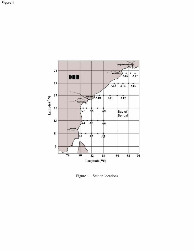
Figure 1 – Station locations

Figure 1

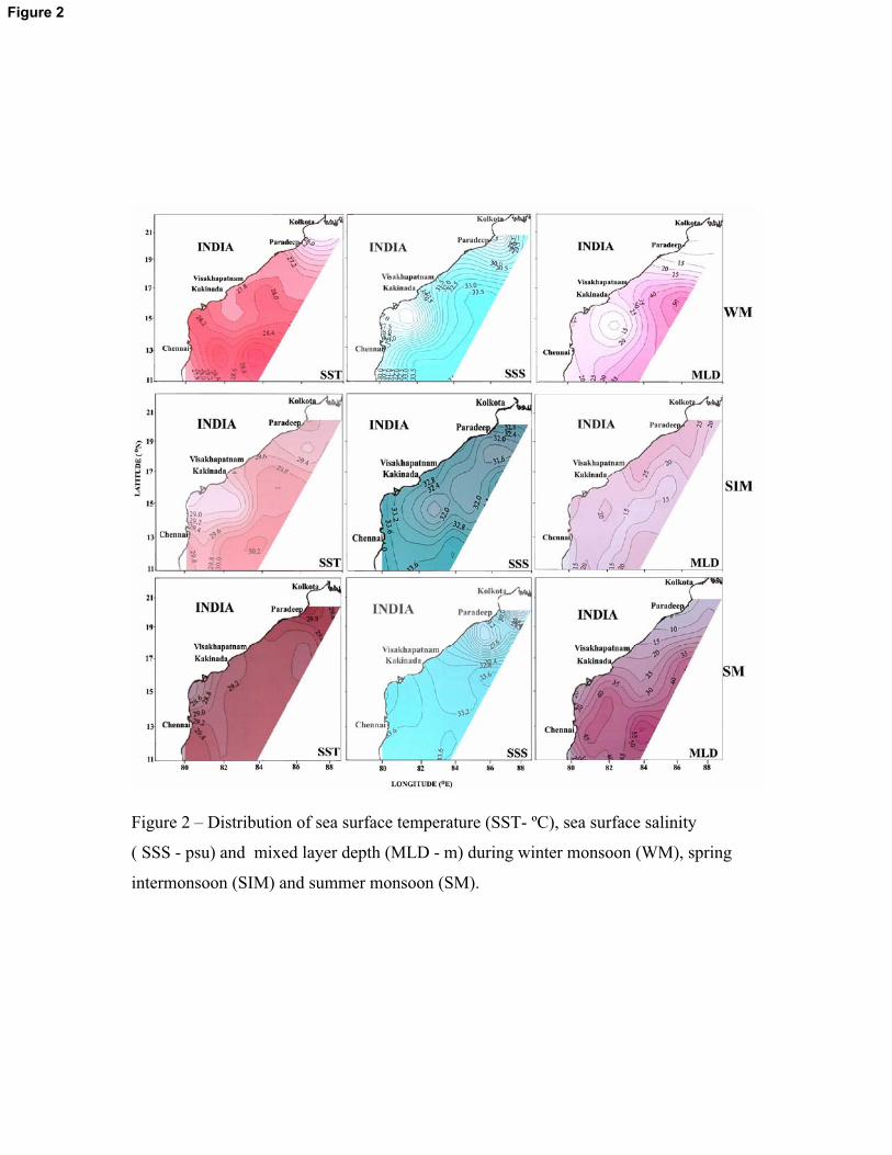
Figure 2 – Distribution of sea surface temperature (SST- ºC), sea surface salinity

( SSS - psu) and mixed layer depth (MLD - m) during winter monsoon (WM), spring

intermonsoon (SIM) and summer monsoon (SM).

Figure 2

11°N 13°N 15°N 17°N 19°N 20.5°N

Euph

otic

col

umn

(m)

0

20

40

60

80

100

120

140

160WM SIM SM

Latitude

11°N 13°N 15°N 17°N 19°N 20.5°N0

20

40

60

80

100

120

140

160WM SIM SM

(a)

(b)

Figure 3 – Seasonal variability of euphotic column in the (a) inshore and (b) oceanic

regions during winter monsoon (WM), spring intermonsoon (SIM) and summer monsoon

(SM).

Figure 3

(a)

(b)

Figure 4 – Cold core eddy signatures (A) Sea level anomalies form Topex/Poseidon (core of the eddy is shown by the pointer) and (B) Vertical structure of temperature (ºC), salinity (psu), and sigma - t (Kg m-

2) along 15ºN transect during winter monsoon

Figure 4

Inshore

-150

-100

-50

0

a

Offshore

b

-150

-100

-50

0

c

------

Dep

th(m

)-----

--

d

11 13 15 17 19-150

-100

-50

0

e

11 13 15 17 19

f

Figure 5 – Vertical distribution of dissolved oxygen during winter monsoon (WM),

spring intermonsoon (SIM) and summer monsoon (SM).

WM

SM

SIM

------Latitude (ºN) --------

Figure 5

-150

-100

-50

0

-150

-100

-50

0

11 13 15 17 19-150

-100

-50

0

11 13 15 17 19

Inshore Offshore

WM

SIM

SM

----

----

Dep

th(m

)---

----

-------- Latitude (°N) --------

Figure 6 – Vertical distribution of nitrate during winter monsoon (WM), spring

intermonsoon (SIM) and summer monsoon (SM).

Figure 6

0.0 0.2 0.4 0.6 0.8 1.0

120

100

80

60

40

20

0

0.0 0.2 0.4 0.6 0.8 1.0

120

10080

60

40

20

00.0 0.2 0.4 0.6 0.8 1.0

120

10080

60

40

20

0

11°N

15°N

0.0 0.2 0.4 0.6 0.8 1.0

120

10080

60

40

20

0

17°N

0.0 0.2 0.4 0.6 0.8 1.0

120

100

80

60

40

20

0

..Chl a (mgm-3)..

...D

epth

(m)..

.

SIM

0.0 0.2 0.4 0.6 0.8 1.0

120

10080

60

40

20

0

SM

WM

Inshore Oceanic

Figure 7 - Vertical distribution of chlorophyll a at representative locations during winter

monsoon (WM), spring intermonsoon (SIM) and summer monsoon (SM).

Figure 7

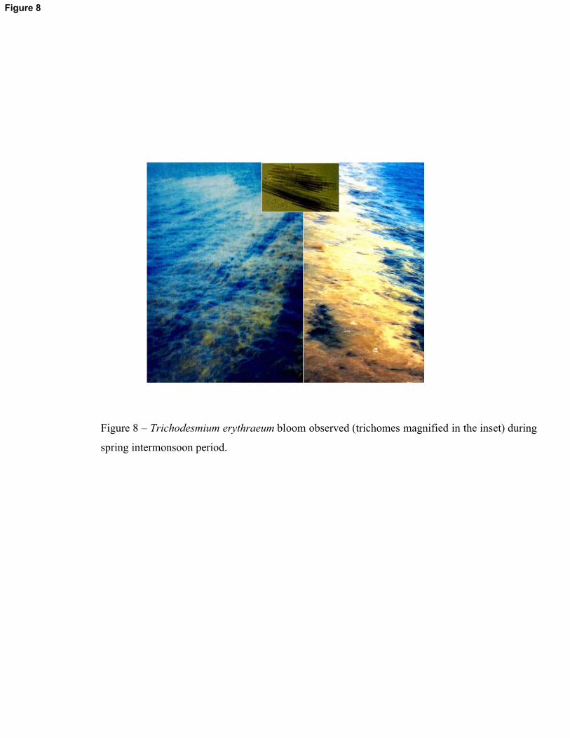
Figure 8 – Trichodesmium erythraeum bloom observed (trichomes magnified in the inset) during

spring intermonsoon period.

Figure 8

WM SIM SM

HDS 70%

CTS 14%

SDS 7%

CNP 9%

HDS 51%

CTS 33%

SDS 7%

CNP 9%

HDS 64%

CTS 19%

SDS 10%

CNP 7%

Figure 9 –Major components of MZP based on abundance during winter monsoon (WM),

spring intermonsoon (SIM) and summer monsoon (SM).

Figure 9

0 50 100 150 200

150

12510075

5025

0

0 50 100 150 200

150125100755025

0

0 50 100 150 200

150125100755025

0

0 50 100 150 200

150125100755025

0

0 50 100 150 200

150125100

755025

0

0 50 100 150 200

15012510075

5025

0

0 50 100 150 200

150125100

755025

0

0 50 100 150 200

150125100755025

0

0 50 100 150 200

150125100

755025

0

InshoreOffshoreOceanic

WM SIM SMMZP abundance (x 103 m-3)

11oN

15oN

19oN

Dep

th(m

)

Figure 10 – Vertical distribution of MZP during winter monsoon (WM), spring intermonsoon (SIM) and

summer monsoon (SM).

Figure 10

0 20 40 60 80

150

125

100

7550

25

00 20 40 60 80

150125100

755025

00 20 40 60 80

150125100

755025

0WM SIM SM

Dep

th(m

)

Abundance (x103 m-3)

HDSCTSSDSCPN

Figure 11 - Seasonal trend in the vertical distribution of heterotrophic dinoflagellates (HDS), ciliates (CTS), sarcordines (SDS) and CPN (copepod nauplii) during winter

monsoon (WM), spring intermonsoon (SIM) and summer monsoon (SM).

Figure 11

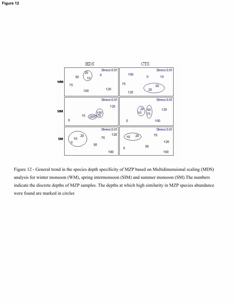
Figure 12 - General trend in the species depth specificity of MZP based on Multidimensional scaling (MDS)

analysis for winter monsoon (WM), spring intermonsoon (SIM) and summer monsoon (SM).The numbers

indicate the discrete depths of MZP samples. The depths at which high similarity in MZP species abundance

were found are marked in circles

Figure 12

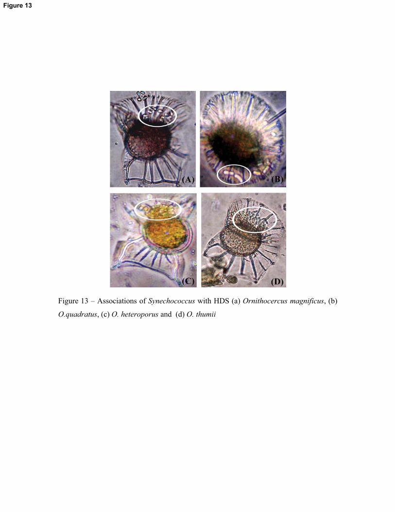
Figure 13 – Associations of Synechococcus with HDS (a) Ornithocercus magnificus, (b)

O.quadratus, (c) O. heteroporus and (d) O. thumii

Figure 13

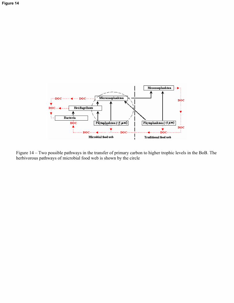
Figure 14 – Two possible pathways in the transfer of primary carbon to higher trophic levels in the BoB. The herbivorous pathways of microbial food web is shown by the circle

Figure 14

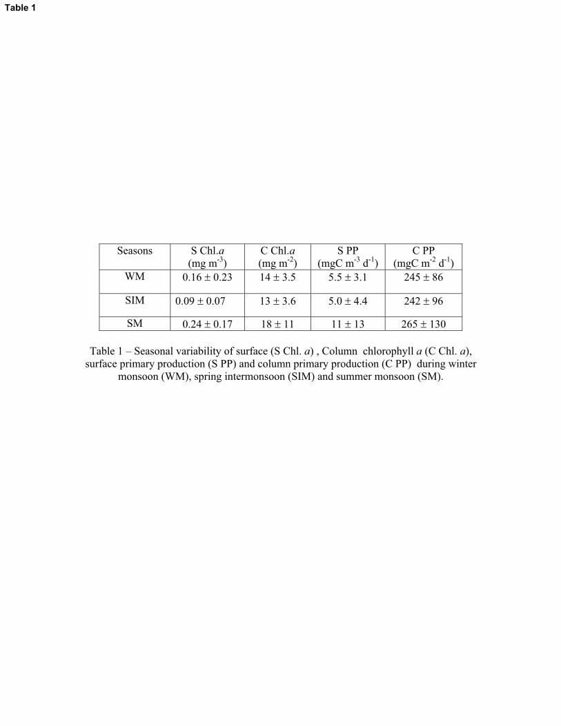
Table 1 – Seasonal variability of surface (S Chl. a) , Column chlorophyll a (C Chl. a), surface primary production (S PP) and column primary production (C PP) during winter

monsoon (WM), spring intermonsoon (SIM) and summer monsoon (SM).

Seasons S Chl.a(mg m-3)

C Chl.a(mg m-2)

S PP(mgC m-3 d-1)

C PP(mgC m-2 d-1)

WM 0.16 � 0.23 14 � 3.5 5.5 � 3.1 245 � 86

SIM 0.09 � 0.07 13 � 3.6 5.0 � 4.4 242 � 96

SM 0.24 � 0.17 18 � 11 11 � 13 265 � 130

Table 1

CTSAmphorella gracilis ( W, I, S) Protorhabdonella simplex ( I, S) O. skogsbergii ( S)

A. intumescens ( W, I, S) Rhabdonella henseni ( W, I) O. steinii ( W, I, S)

A. pachytoecus ( W, I, S) R. spiralis ( W, I, S) O. thumii ( W, I, S)

A. quadrilineata ( W, I, S) R. amor ( W, I, S) Parahistioneis para ( W, I)

A. tetragona (I, S) R. elegans ( W, I, S) Phalacroma doryphorum ( W, I, S)

Amphorellopsis acuta (I, S) R. longicaulis (I, S) P. purvula ( W, I, S)

Amphorides minor (I) R. poculum ( I) P. sp. ( S)

Amplectella sp. (W, I ,S) Salpingacantha ampla ( W, I, S) P. cuneus ( W, I)

Ascambelliella armila (I ) S. sp. ( W, I, S) P. favus ( W, I, S)

A. retrusa ( W, I, S) Salpingella acuminata ( W, I, S) P. mitra (I, S)

Brandtiella palliada ( W, I, S) Salpingella attenuata ( W, I, S) P. rapa ( W, I, S)

Canthariella pyramidata ( W, I, S) S. decurtata ( I, S) Podolampas bipes ( W, I, S)

Codonella acera ( W, I, S) S. gracilis ( I, S) P. elegans ( W, I, S)

C. amphorella ( W, I, S) S. stenostoma ( W, I, S) P. palmipes (I, S)

C. nationalis ( W, I, S) Steenstrupiella pozzi ( I, S) P. reticulata ( W, S)

Codonellopsis ecaudata( W, I) S. steenstrupii ( I, S) P. spinifera ( W, I, S)

C. minor ( W, I, S) Stenosemella ventricosa ( I) Protoperidinium breve ( W, S)

C. morchella ( I, S) Strombidium bilobum ( W, I, S) P. brevipes ( S)

C. nipponica ( I, S) S. conicum ( I, S) P. conicum ( W, I)

C. orthoceras ( I, S) Strobilidium minimum ( W, I, S) P. crassipes ( W, I, S)

C. ostenfeldi ( W, I, S) Tintinnopsis beroidea (I, S) P. curtips ( W, I, S)

C. tessellata ( I, S) T. butschli ( I) P. depressum ( W, S)

Cyttarocylis acutiformes ( I, S) T. cylindrical ( W, I, S) P. divergens ( W, I, S)

Dadayiella ganymedes ( I, S) T. directa ( W, I, S) P. elegans ( W, I, S)

D. pachytoecus ( I) T. incertum ( I, S) P. fatulipes ( W, I, S)

Dictyocysta duplex ( W, I, S) T. mortenseni ( I, S) P. globules ( W, I, S)

D. elegans ( W, I, S) T. radix ( W, I, S) P. grandae ( W, I)

D. lepida ( I, S) T. tocantinensis ( W, I, S) P. granii ( W, I)

Epiplocycloids reticulata ( I) Undella dialata ( W, I, S) P. heteracanthum ( W, I, S)

Epiplocylis undella ( W, I, S) U. globosa ( W, I, S) P. latistriatum ( W, S)

Eutintinnus elongates ( W, I, S) U. hyaline ( W, I, S) P. leonis ( W, I, S)

E. fraknoi ( W, I, S) Xystonella treforti ( W, I, S) P. longicollum ( S)

E. lusus undae ( W, I, S) HDS P. longipes ( W, I, S)

E.tineus ( W, I, S) Dinophysis acuta ( W, I, S) P. nipponicum ( I, S)

Favella brevis ( I) D. apicata ( W, I, S) P. oblongum ( I)Halteria chlorelligera ( I) D. hastate ( W, I, S) P. oceanicum ( W, I, S)

Helicostomella subulata ( I) Diplopsalis lenticula ( W, I, S) P. ovatum ( S)

Leprotintinnus nordquisti ( W, I, S) Gymnodinium abbreviatum ( W, I, S) P. ovum ( I, S)

Lohmaniella oviformis ( I, S) Gyrodinium sp. ( W, I, S) P. pellucidum ( W, I, S)

L. spiralis ( I) Heterodinium blackmanii ( W, I, S) P.quarnerese ( W, I, S)

Metacylis jorgenseni ( I) Histioneis hyaline ( W, I, S) P. steinii ( W, I, S)

Parundella caudate ( I) H. striata ( W, I, S) P. tuba ( W, I, S)

P. lohmani ( W, I, S) Noctiluca scintillans ( W, I, S) P. pentagonum ( W, I, S)

Petalotricha ampulla ( W, I, S) Ornithocercus heteroporus ( W, I) P. claudicans ( I, S)

P. serrata ( I) O. magnificus ( W, I, S)

Proplectella claparedi ( I) O. quadratus ( W, I, S)

Table 2 – Seasonal variability in the MZP species (W – WM, I – SIM, S – SM)

Table 2

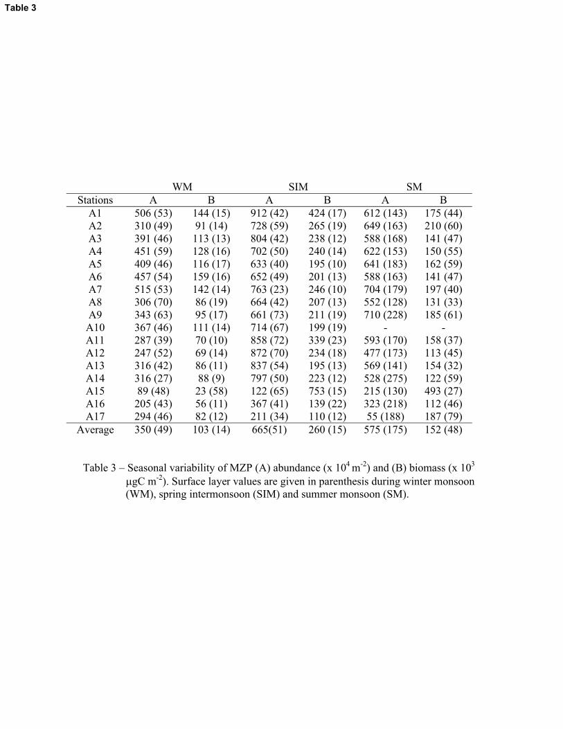
WM SIM SMStations A B A B A B

A1 506 (53) 144 (15) 912 (42) 424 (17) 612 (143) 175 (44)A2 310 (49) 91 (14) 728 (59) 265 (19) 649 (163) 210 (60)A3 391 (46) 113 (13) 804 (42) 238 (12) 588 (168) 141 (47)A4 451 (59) 128 (16) 702 (50) 240 (14) 622 (153) 150 (55)A5 409 (46) 116 (17) 633 (40) 195 (10) 641 (183) 162 (59)A6 457 (54) 159 (16) 652 (49) 201 (13) 588 (163) 141 (47)A7 515 (53) 142 (14) 763 (23) 246 (10) 704 (179) 197 (40)A8 306 (70) 86 (19) 664 (42) 207 (13) 552 (128) 131 (33)A9 343 (63) 95 (17) 661 (73) 211 (19) 710 (228) 185 (61)A10 367 (46) 111 (14) 714 (67) 199 (19) - -A11 287 (39) 70 (10) 858 (72) 339 (23) 593 (170) 158 (37)A12 247 (52) 69 (14) 872 (70) 234 (18) 477 (173) 113 (45)A13 316 (42) 86 (11) 837 (54) 195 (13) 569 (141) 154 (32)A14 316 (27) 88 (9) 797 (50) 223 (12) 528 (275) 122 (59)A15 89 (48) 23 (58) 122 (65) 753 (15) 215 (130) 493 (27)A16 205 (43) 56 (11) 367 (41) 139 (22) 323 (218) 112 (46)A17 294 (46) 82 (12) 211 (34) 110 (12) 55 (188) 187 (79)

Average 350 (49) 103 (14) 665(51) 260 (15) 575 (175) 152 (48)

Table 3 – Seasonal variability of MZP (A) abundance (x 104 m-2) and (B) biomass (x 103

�gC m-2). Surface layer values are given in parenthesis during winter monsoon (WM), spring intermonsoon (SIM) and summer monsoon (SM).

Table 3

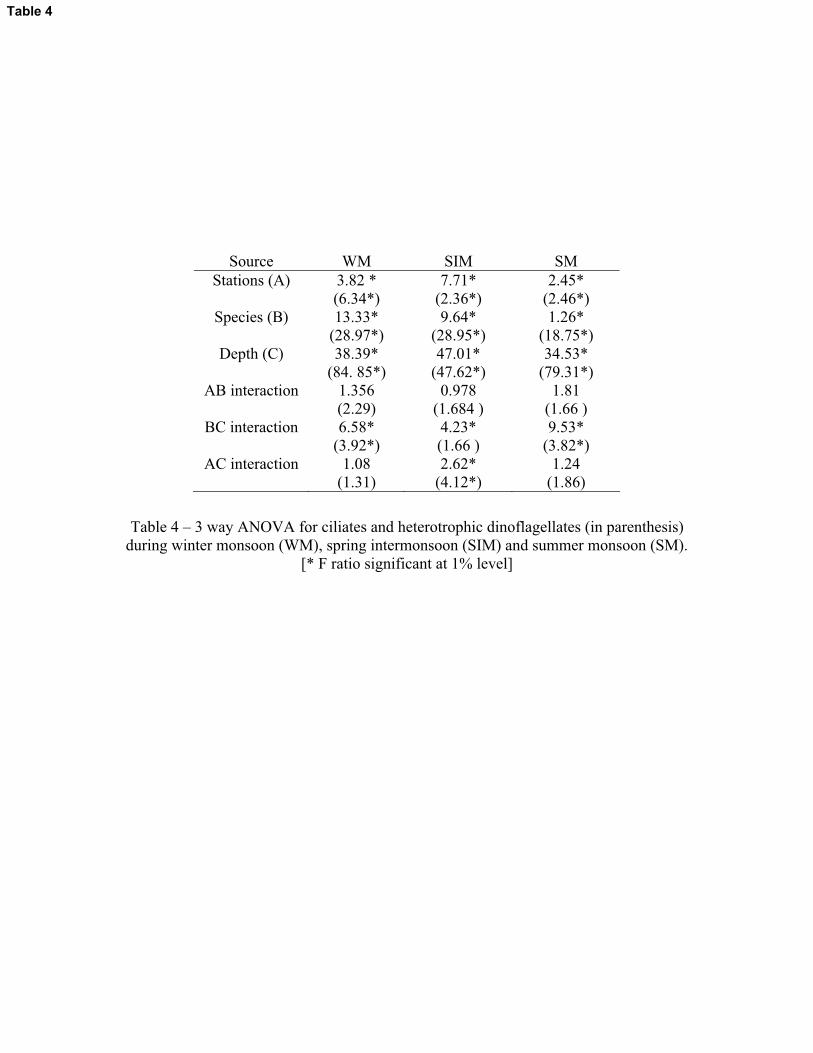
Table 4 – 3 way ANOVA for ciliates and heterotrophic dinoflagellates (in parenthesis)during winter monsoon (WM), spring intermonsoon (SIM) and summer monsoon (SM).

[* F ratio significant at 1% level]

Source WM SIM SMStations (A) 3.82 *

(6.34*)7.71*

(2.36*)2.45*

(2.46*)Species (B) 13.33*

(28.97*)9.64*

(28.95*)1.26*

(18.75*)Depth (C) 38.39*

(84. 85*)47.01*

(47.62*)34.53*

(79.31*)AB interaction 1.356

(2.29)0.978

(1.684 )1.81

(1.66 )BC interaction 6.58*

(3.92*)4.23*(1.66 )

9.53*(3.82*)

AC interaction 1.08(1.31)

2.62*(4.12*)

1.24(1.86)

Table 4

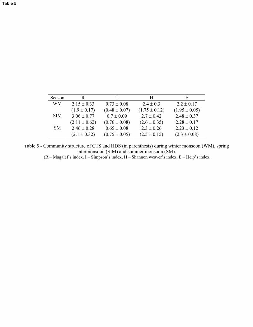
Season R I H EWM 2.15 � 0.33

(1.9 � 0.17)0.73 � 0.08

(0.48 � 0.07)2.4 � 0.3

(1.75 � 0.12)2.2 � 0.17

(1.95 � 0.05)SIM 3.06 � 0.77

(2.11 � 0.62)0.7 � 0.09

(0.76 � 0.08)2.7 � 0.42

(2.6 � 0.35)2.48 � 0.372.28 � 0.17

SM 2.46 � 0.28(2.1 � 0.32)

0.65 � 0.08(0.75 � 0.05)

2.3 � 0.26(2.5 � 0.15)

2.23 � 0.12(2.3 � 0.08)

Table 5 - Community structure of CTS and HDS (in parenthesis) during winter monsoon (WM), spring intermonsoon (SIM) and summer monsoon (SM).

(R – Magalef’s index, I – Simpson’s index, H – Shannon weaver’s index, E – Heip’s index

Table 5

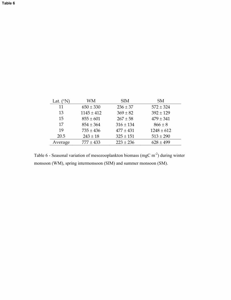
Table 6 - Seasonal variation of mesozooplankton biomass (mgC m-2) during winter

monsoon (WM), spring intermonsoon (SIM) and summer monsoon (SM).

Lat. (�N) WM SIM SM11 650 � 330 236 � 37 572 � 32413 1145 � 412 369 � 82 392 � 12915 855 � 601 267 � 58 479 � 34117 854 � 364 316 � 134 866 � 819 735 � 436 477 � 431 1248 � 612

20.5 243 � 18 325 � 151 513 � 290Average 777 � 433 223 � 236 628 � 499

Table 6