THE 8 μm PHASE VARIATION OF THE HOT SATURN HD …showman/publications/knutson-etal-2009b.pdf ·...
16
The Astrophysical Journal, 703:769–784, 2009 September 20 doi:10.1088/0004-637X/703/1/769 C 2009. The American Astronomical Society. All rights reserved. Printed in the U.S.A. THE 8 μm PHASE VARIATION OF THE HOT SATURNHD 149026b Heather A. Knutson 1 , David Charbonneau 1 , Nicolas B. Cowan 2 , Jonathan J. Fortney 3 , Adam P. Showman 4 , Eric Agol 2 , and Gregory W. Henry 5 1 Harvard-Smithsonian Center for Astrophysics, 60 Garden St., Cambridge, MA 02138, USA; [email protected] 2 Department of Astronomy, Box 351580, University of Washington, Seattle, WA 98195, USA 3 Department of Astronomy and Astrophysics, UCO/Lick Observatory, University of California, Santa Cruz, CA 95064, USA 4 Lunar and Planetary Laboratory and Department of Planetary Sciences, University of Arizona, Tucson, AZ 85721, USA 5 Center of Excellence in Information Systems, Tennessee State University, 3500 John A. Merritt Blvd., Box 9501, Nashville, TN 37209, USA Received 2009 May 22; accepted 2009 August 6; published 2009 September 1 ABSTRACT We monitor the star HD 149026 and its Saturn-mass planet at 8.0 μm over slightly more than half an orbit using the Infrared Array Camera on the Spitzer Space Telescope. We find an increase of 0.0227% ± 0.0066% (3.4σ significance) in the combined planet–star flux during this interval. The minimum flux from the planet is 45% ± 19% of the maximum planet flux, corresponding to a difference in brightness temperature of 480 ± 140 K between the two hemispheres. We derive a new secondary eclipse depth of 0.0411% ± 0.0076% in this band, corresponding to a dayside brightness temperature of 1440 ± 150 K. Our new secondary eclipse depth is half that of a previous measurement (3.0σ difference) in this same bandpass by Harrrington et al. We re-fit the Harrrington et al. data and obtain a comparably good fit with a smaller eclipse depth that is consistent with our new value. In contrast to earlier claims, our new eclipse depth suggests that this planet’s dayside emission spectrum is relatively cool, with an 8 μm brightness temperature that is less than the maximum planet-wide equilibrium temperature. We measure the interval between the transit and secondary eclipse and find that that the secondary eclipse occurs 20.9 +7.2 −6.5 minutes earlier (2.9σ ) than predicted for a circular orbit, a marginally significant result. This corresponds to e cos (ω) =−0.0079 +0.0027 −0.0025 , where e is the planet’s orbital eccentricity and ω is the argument of pericenter. Key words: eclipses – planetary systems – stars: individual (HD 149026b) – techniques: photometric 1. INTRODUCTION The planet orbiting HD 149026 is unique among the ranks of transiting extrasolar planets. It has a mass comparable to that of Saturn (Sato et al. 2005; Winn et al. 2008; Carter et al. 2009) but its small radius and correspondingly high average density (Sato et al. 2005; Charbonneau et al. 2006; Winn et al. 2008; Nutzman et al. 2009; Carter et al. 2009) suggest that, unlike Saturn, an incredible 50%–90% of this planet’s mass must exist in the form of a solid icy or rocky core (Sato et al. 2005; Fortney et al. 2006; Ikoma et al. 2006; Broeg & Wuchterl 2007; Burrows et al. 2007a). Together with the Neptune-mass planets GJ 436b (Butler et al. 2004; Gillon et al. 2007) and HAT-P-11b (Bakos et al. 2009), this places HD 149026b in a class that is distinct from that of the more massive “hot Jupiter” transiting planets with their primarily hydrogen–helium compositions. In light of its large rock or ice core, it is possible that HD 149026b also has an atmospheric composition that differs significantly from those of the hot Jupiters. In the solar system, there is a correlation between atmospheric metallicity and the percentage of planet mass that is core (e.g., Lodders 2003). For example, Uranus and Neptune have a C/H ratio of 30–40 times solar while Jupiter’s is roughly three times solar. If this relation holds true for extrasolar planets, it would suggest that HD 149026b may have a significantly metal- enriched atmosphere. The HD 149026 primary is also metal enriched ([Fe/H] = 0.36 ± 0.05; Sato et al. 2005), thus even if HD 149026b’s atmosphere simply reflects the composition of its primordial nebula we would expect it to have a slightly higher heavy metal content than a typical hot Jupiter. By observing the decrease in light as the planet passes behind its parent star in an event known as a secondary eclipse, we can characterize the properties of HD 149026b’s dayside emission spectrum. Harrington et al. (2007, hereafter H07) measured HD 149026b’s secondary eclipse at 8 μm and found a depth of 0.084% +0.009% −0.012% , corresponding to a brightness temperature 6 of 2300 ± 200 K for the planet. This is significantly higher than expected, as HD 149026b has an equilibrium temperature 7 of only 1740 K (H07). In order to reproduce this flux in the case where the planet emits as a blackbody, we must assume that the planet absorbs and then instantaneously re-radiates all of the incident flux from its star on the dayside. In this scenario, the planet’s nightside would have effectively zero flux; this follows from the requirement that the energy emitted by the planet does not exceed the energy it absorbs (note that residual heat from formation is not expected to play a significant role in the energy budgets of close-in planets). This is not unreasonable, as the timescale for tidal locking of close-in planets such as HD 149026b is considerably shorter than the ages of these systems (Guillot et al. 1996; Lubow et al. 1997). Uneven irradiation of the upper atmosphere could produce a large observed day–night temperature gradient if radiative timescales are much less than advective timescales at the level of the mid- IR photosphere (i.e., flux is absorbed and re-emitted by gas on the dayside in less time than it takes that same parcel of gas to reach the nightside hemisphere). If the planet’s spectrum differs significantly from that of a blackbody with enhanced emission at 8 μm, the constraints on the nightside emission becomes 6 Brightness temperature is defined in this case as the temperature required to match the observed planet–star flux ratio in the 8 μm Spitzer IRAC bandpass assuming that the planet radiates as a blackbody and using a Kurucz atmosphere model for the star. 7 Equilibrium temperature is calculated by assuming that the planet absorbs all incident flux (i.e., zero albedo) and then re-radiates that energy over its entire surface as a blackbody of the stated temperature. 769
Transcript of THE 8 μm PHASE VARIATION OF THE HOT SATURN HD …showman/publications/knutson-etal-2009b.pdf ·...
The Astrophysical Journal, 703:769–784, 2009 September 20 doi:10.1088/0004-637X/703/1/769C© 2009. The American Astronomical Society. All rights reserved. Printed in the U.S.A.
THE 8 μm PHASE VARIATION OF THE HOT SATURN HD 149026b
Heather A. Knutson1, David Charbonneau
1, Nicolas B. Cowan
2, Jonathan J. Fortney
3, Adam P. Showman
4,
Eric Agol2, and Gregory W. Henry
51 Harvard-Smithsonian Center for Astrophysics, 60 Garden St., Cambridge, MA 02138, USA; [email protected]
2 Department of Astronomy, Box 351580, University of Washington, Seattle, WA 98195, USA3 Department of Astronomy and Astrophysics, UCO/Lick Observatory, University of California, Santa Cruz, CA 95064, USA
4 Lunar and Planetary Laboratory and Department of Planetary Sciences, University of Arizona, Tucson, AZ 85721, USA5 Center of Excellence in Information Systems, Tennessee State University, 3500 John A. Merritt Blvd., Box 9501, Nashville, TN 37209, USA
Received 2009 May 22; accepted 2009 August 6; published 2009 September 1
ABSTRACT
We monitor the star HD 149026 and its Saturn-mass planet at 8.0 μm over slightly more than half an orbit usingthe Infrared Array Camera on the Spitzer Space Telescope. We find an increase of 0.0227% ± 0.0066% (3.4σsignificance) in the combined planet–star flux during this interval. The minimum flux from the planet is 45%±19%of the maximum planet flux, corresponding to a difference in brightness temperature of 480 ± 140 K between thetwo hemispheres. We derive a new secondary eclipse depth of 0.0411% ± 0.0076% in this band, correspondingto a dayside brightness temperature of 1440 ± 150 K. Our new secondary eclipse depth is half that of a previousmeasurement (3.0σ difference) in this same bandpass by Harrrington et al. We re-fit the Harrrington et al. dataand obtain a comparably good fit with a smaller eclipse depth that is consistent with our new value. In contrastto earlier claims, our new eclipse depth suggests that this planet’s dayside emission spectrum is relatively cool,with an 8 μm brightness temperature that is less than the maximum planet-wide equilibrium temperature. Wemeasure the interval between the transit and secondary eclipse and find that that the secondary eclipse occurs20.9+7.2
−6.5 minutes earlier (2.9σ ) than predicted for a circular orbit, a marginally significant result. This correspondsto e cos (ω) = −0.0079+0.0027
−0.0025, where e is the planet’s orbital eccentricity and ω is the argument of pericenter.
Key words: eclipses – planetary systems – stars: individual (HD 149026b) – techniques: photometric
1. INTRODUCTION
The planet orbiting HD 149026 is unique among the ranks oftransiting extrasolar planets. It has a mass comparable to that ofSaturn (Sato et al. 2005; Winn et al. 2008; Carter et al. 2009)but its small radius and correspondingly high average density(Sato et al. 2005; Charbonneau et al. 2006; Winn et al. 2008;Nutzman et al. 2009; Carter et al. 2009) suggest that, unlikeSaturn, an incredible 50%–90% of this planet’s mass must existin the form of a solid icy or rocky core (Sato et al. 2005; Fortneyet al. 2006; Ikoma et al. 2006; Broeg & Wuchterl 2007; Burrowset al. 2007a). Together with the Neptune-mass planets GJ 436b(Butler et al. 2004; Gillon et al. 2007) and HAT-P-11b (Bakoset al. 2009), this places HD 149026b in a class that is distinctfrom that of the more massive “hot Jupiter” transiting planetswith their primarily hydrogen–helium compositions.
In light of its large rock or ice core, it is possible thatHD 149026b also has an atmospheric composition that differssignificantly from those of the hot Jupiters. In the solar system,there is a correlation between atmospheric metallicity andthe percentage of planet mass that is core (e.g., Lodders2003). For example, Uranus and Neptune have a C/H ratioof 30–40 times solar while Jupiter’s is roughly three timessolar. If this relation holds true for extrasolar planets, it wouldsuggest that HD 149026b may have a significantly metal-enriched atmosphere. The HD 149026 primary is also metalenriched ([Fe/H] = 0.36 ± 0.05; Sato et al. 2005), thus evenif HD 149026b’s atmosphere simply reflects the compositionof its primordial nebula we would expect it to have a slightlyhigher heavy metal content than a typical hot Jupiter.
By observing the decrease in light as the planet passes behindits parent star in an event known as a secondary eclipse, we cancharacterize the properties of HD 149026b’s dayside emission
spectrum. Harrington et al. (2007, hereafter H07) measuredHD 149026b’s secondary eclipse at 8 μm and found a depthof 0.084%+0.009%
−0.012%, corresponding to a brightness temperature6
of 2300 ± 200 K for the planet. This is significantly higher thanexpected, as HD 149026b has an equilibrium temperature7 ofonly 1740 K (H07). In order to reproduce this flux in the casewhere the planet emits as a blackbody, we must assume thatthe planet absorbs and then instantaneously re-radiates all of theincident flux from its star on the dayside. In this scenario, theplanet’s nightside would have effectively zero flux; this followsfrom the requirement that the energy emitted by the planetdoes not exceed the energy it absorbs (note that residual heatfrom formation is not expected to play a significant role in theenergy budgets of close-in planets). This is not unreasonable,as the timescale for tidal locking of close-in planets such asHD 149026b is considerably shorter than the ages of thesesystems (Guillot et al. 1996; Lubow et al. 1997). Unevenirradiation of the upper atmosphere could produce a largeobserved day–night temperature gradient if radiative timescalesare much less than advective timescales at the level of the mid-IR photosphere (i.e., flux is absorbed and re-emitted by gas onthe dayside in less time than it takes that same parcel of gas toreach the nightside hemisphere). If the planet’s spectrum differssignificantly from that of a blackbody with enhanced emissionat 8 μm, the constraints on the nightside emission becomes
6 Brightness temperature is defined in this case as the temperature required tomatch the observed planet–star flux ratio in the 8 μm Spitzer IRAC bandpassassuming that the planet radiates as a blackbody and using a Kuruczatmosphere model for the star.7 Equilibrium temperature is calculated by assuming that the planet absorbsall incident flux (i.e., zero albedo) and then re-radiates that energy over itsentire surface as a blackbody of the stated temperature.
769
770 KNUTSON ET AL. Vol. 703
correspondingly less stringent. If we compare HD 149026b’s8 μm flux to the predictions from one-dimensional atmospheremodels for the planet (e.g., Fortney et al. 2006; Burrows et al.2008a), we find that models with a temperature inversion andwater features in emission at 8 μm still require a hot dayside andcorrespondingly large day–night temperature gradient in orderto match the 8 μm flux observed by H07.
In this paper, we characterize HD 149026b’s 8 μm phasevariation and corresponding day–night temperature gradient bymonitoring the system continuously over slightly more than halfan orbit, beginning before the transit and ending after the sec-ondary eclipse. By measuring the increase in brightness as theplanet’s dayside rotates into view, we can estimate the day–nighttemperature gradient and constrain corresponding atmosphericcirculation models for the planet. We have previously publishedsimilar observations of HD 189733b at 8 and 24 μm (Knutsonet al. 2007, 2009b) where we invert the observed phase varia-tion to produce a longitudinal temperature profile for the planet.These observations revealed that HD 189733b has a warm night-side (approximately 250 K cooler than the 1250 K dayside), butlower-cadence observations of the non-transiting planets υ Andb (Harrington et al. 2006) and HD 179949b (Cowan et al. 2007)suggest that other hot Jupiters may have large day–night tem-perature gradients. HD 149026b’s lower mass and increasedcore fraction make it qualitatively different than any of thesesystems, and there are no published general circulation modelsfor this planet analogous to those available for HD 189733b andHD 209458b (e.g., Showman et al. 2009). As a result, we haveno a priori predictions for the nature of the day–night circula-tion on HD 149026b other than the constraint provided by thesecondary eclipse measurement of H07.
These same data also allow us to search for time-varying prop-erties of the system by comparing the depths and relative timesof our transit and secondary eclipse to previously published8 μm Spitzer observations of the planet’s transit (Nutzman et al.2009, obtained in 2007) and secondary eclipse (H07, obtainedin 2005). If the planet’s orbit is changing over time, perhapsas the result of interactions with an unknown second planet inthe system, it could cause deviations in the timing of successivetransits (Miralda-Escude 2002; Holman & Murray 2005; Agolet al. 2005). Comparing our 8 μm planet–star radius ratio tothe value obtained by Nutzman et al. (2009) allows us to searchfor changes in the effective radius of the planet at 8 μm and,if the two values are consistent, obtain an improved estimatefor this quantity. By measuring the interval between the transitand secondary eclipse, we can determine a value for e cos(ω)where e is the planet’s orbital eccentricity and ω is the argu-ment of pericenter, and compare it to the corresponding valuefrom H07. Finally, by comparing the 8 μm secondary eclipsedepth from our observations to that of H07, we can search forvariations in the planet’s 8 μm dayside flux.
In Section 2, we describe our treatment of the data, includingour initial photometry, the use of a new preflash technique toremove the detector ramp, and our fits to the transit, secondaryeclipse, and phase curve data. In Section 3, we discuss theresults of these fits and check for variability in the relativedepth and timing of our transit and secondary eclipse ascompared to previously published data. We also compareour day- and nightside fluxes to the predictions from one-dimensional atmosphere models and calculate an energy budgetfor the planet. In Section 4, we summarize our results and discussthe potential impact of upcoming observations of this planet’ssecondary eclipse and phase curve at shorter wavelengths.
2. OBSERVATIONS
We monitored HD 149026b continuously for 41 hr using8 μm Infrared Array Camera (IRAC) subarray (Fazio et al.2004) on the Spitzer Space Telescope (Werner et al. 2004), fromUT 2008 May 11 to 12. Our observations began 2.5 hr beforethe start of the transit and finished 44 minutes after the end ofthe secondary eclipse. We used an integration time of 0.4 s, wellbelow saturation for this star, and obtained a total of 344,704images.
2.1. Initial Photometry
Because HD 149026 is a bright star (K = 6.819, one-thirdthe brightness of HD 189733 in the infrared) relative to thebackground at these wavelengths, we calculate the flux fromthe star in each image using aperture photometry with a radiusof 3.5 pixels. We determine the position of the star in eachimage as the position-weighted sum of the flux in a circularregion with a radius of 5 pixels (rounded to the nearest pixel)centered on the approximate position of the star. We calculateposition estimates with larger and smaller apertures, but findthat a 5-pixel aperture produced the lowest rms in the resultingtime series. Similarly, we find that decreasing our photometricapertures to values smaller than 3.5 pixels led to position-dependent flux losses, while the time series from larger aperturesbecome increasingly noisy. We repeat our analysis for aperturesranging from 3.5 to 7 pixels and find that our results for themeasured secondary eclipse depth and phase variation amplitudeare consistent in all cases. We also try fitting a point-spreadfunction (PSF) to the images, using either the in-flight pointresponse functions generated from calibration test data8 or aPSF derived from our own data, and conclude that aperturephotometry produces the optimal results.
Because the subarray is only 32×32 pixels, care is needed inthe choice of regions for background flux estimates. We excludeall pixels within a circular region with a radius of 9 pixelscentered on the position of the star, as well as the top rowof the array which has consistently low-flux values, and trim3σ outliers from the remaining set of pixels. We then make ahistogram of the fluxes in the remaining pixels and fit a Gaussianfunction to the central 7 of 10 bins in this distribution (furtherreducing the effects of any remaining high- or low-flux outliersin the distribution) to estimate the mean background level ineach individual image. We obtain identical results if we includethe top row of pixels, increase the size of the exclusion regionin the center of the array, or exclude an additional four rowsfrom y = 11–16 corresponding to particularly bright diffractionspikes on the star’s PSF. We find that the background flux duringour observations is consistently below zero, with a median valueof −0.053 MJy sr−1, suggesting that the sky dark used forthese observations is oversubtracting the background. This hasno effect on our final photometry provided that the negativebackground value is correctly subtracted from each image beforeestimating the flux from HD 149026.
We calculate the JD value for each image as the time at mid-exposure, and apply a correction to convert these JD values to theappropriate BJD, taking into account Spitzer’s orbital position ateach point during the observations. The background and stellarfluxes in the first 10 images and the 58th image in each set of64 have consistently lower values than the rest of the exposures,
8 Available at http://ssc.spitzer.caltech.edu/irac/psf.html
No. 1, 2009 THE 8 μm PHASE VARIATION OF THE HOT SATURN HD 149026b 771
100 101 102 103 104 105
Bin Size
10-5
10-4
10-3
10-2R
MS
of
Bin
ne
d R
esi
du
als
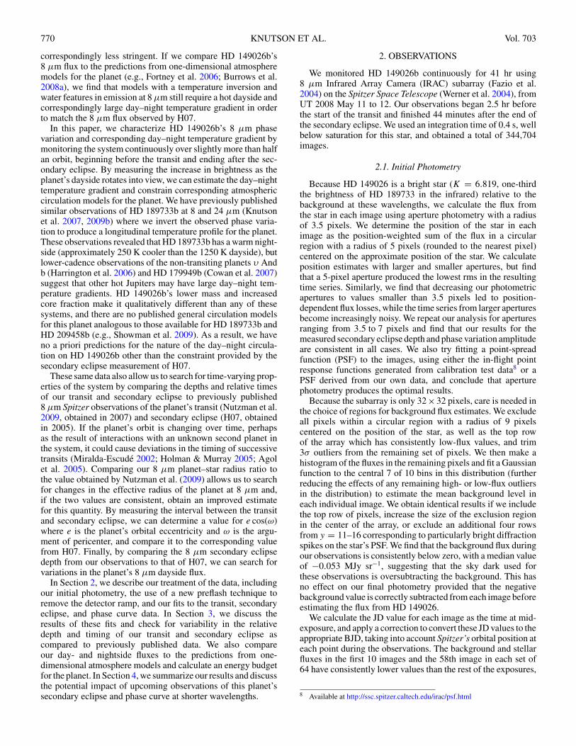
Figure 1. rms of the time series between the end of the transit and the start of thesecondary eclipse (10 < dt < 35 hr) over a range of bin sizes (black line, binsup to 50,000 points). We have fitted and removed a linear function of time fromthese data to correct for the effects of the planet’s phase variation before binningthe data and calculating the resulting rms. The solid red line shows the rms ofthe unbinned data scaled by
√n where n is the number of points in each bin.
The increased noise for bin sizes between 1000 and 4000 points (10–30 minutetimescales) may be related to the pointing jitter of the telescope, which shiftsback and forth by approximately 0.1 pixels in x and y over 1 hr cycles. Althoughwe find no evidence for a direct relation between the measured x/y positions ofthe star on the array and the corresponding stellar fluxes, the fact that this excessnoise disappears for bin sizes larger than 8000 points (1 hr intervals) suggeststhese two phenomena may be related.
but we find that this behavior disappears after the backgroundis subtracted. As a check, we exclude these low frames andrepeat our analysis, and find that we obtain consistent results(secondary eclipse depth and phase variation amplitude) in bothcases. We include these frames in our final analysis.
Our final time series has a number of high-flux outliersproduced by the presence of transient hot pixels in the array.We remove these points by discarding images where the xposition, y position, or total flux from the star in a 3.5-pixelaperture differed by more than 3σ from the median value forthese quantities in each set of 64 images (because we calculatethe star’s position as the position-weighted sum of the flux ina given region, transient hot pixels may affect these estimateseven if they are not included in the final photometry). We trim0.78% of the images using this method, and see no evidence forremaining outliers in the final time series. We calculate the rmsof the points in each bins in the phase curve plotted in Figure 7and find that the average rms in these bins is 0.826%, whichis a factor of 1.27 higher than the predicted photon noise fromthe star alone (we do not include the noise contribution fromthe background flux because this flux is negative in our images,and we do not have a reliable estimate of its true value with acorrect sky dark subtraction). This is consistent with previousSpitzer photometry in this bandpass for GJ 436, HD 149026, andHD 189733 (Deming et al. 2007; H07; Knutson et al. 2007), allof which have roughly comparable fluxes in this bandpass. Wefind that this noise is reasonably white; Figure 1 shows the rmsof the time series between the end of the transit and the startof the secondary eclipse (10 < dt < 35 hr) over a range ofbin sizes up to 50,000 points after the data have fitted with alinear function of time which was then removed to ensure thatthe real astrophysical change in the planet’s flux does not inflatethe resulting rms estimates.
2.2. Preflashing and the Detector Ramp Effect
After determining the optimal method for estimating thefluxes in each bandpass, we must remove any remaining de-tector effects from the data. There is a well-documented detec-tor effect (H07; Knutson et al. 2007, 2008; Charbonneau et al.2008) in this array that causes the effective gain (and thus themeasured flux) in individual pixels to increase over time. Thiseffect has been referred to as the “detector ramp,” and has alsobeen observed to occur in the IRS 16 μm peak-up and MIPS24 μm arrays, which are made from the same material (Deminget al. 2006; Charbonneau et al. 2008). The IRAC 5.8 μm arrayalso shows a related behavior, with an initial upward asymptotein the measured flux over the first 30–60 minutes of observa-tion followed by a more gradual downward slope (Charbonneauet al. 2008; Knutson et al. 2008, 2009a; Machalek et al. 2008).The size of this effect depends on the illumination level of theindividual pixel. Pixels with high illuminations (>250 MJy sr−1
in the 8 μm channel) will converge to a constant value withinthe first hour of observations, whereas lower-illumination pixelswill show a linear increase in the measured flux over time witha slope that varies inversely with the logarithm of the illumi-nation level. It has been suggested that this effect may be theresult of charge trapping in the array, with higher-illuminationpixels filling their wells more quickly than lower-illuminationpixels.
We mitigated this effect by observing M17, a nearby opencluster with diffuse bright emission at 8 μm, centered on theposition α = 18h20m28.s0, δ = −16◦12′19.′′5 for 32 minutesimmediately prior to the start of our science observations.This preflash is designed to saturate out the ramp effect byexposing the array to a uniformly bright source with fluxesthat are approximately 10× higher than the peak flux in thecenter of HD 149026’s PSF. The region of M17 that we use forour preflash has fluxes between 3500 and 8000 MJy sr−1 in theIRAC 8 μm subarray aperture, with an average flux of 7400 MJysr−1 in a circular region with a radius of 3.5 pixels centered on theposition of HD 149026 in our science images. We use the sameexposure time and subarray observing mode for our preflashthat we use for our observations of HD 149026, obtaining atotal of 4480 preflash images. The peak flux in these imagesoccurs at the position of a star in the corner of the array with amaximum flux of 13,000 MJy sr−1 or 100,000e−, correspondingto half of the full well depth in this array. Because we are wellbelow saturation, we do not expect any latency effects in oursubsequent science images.
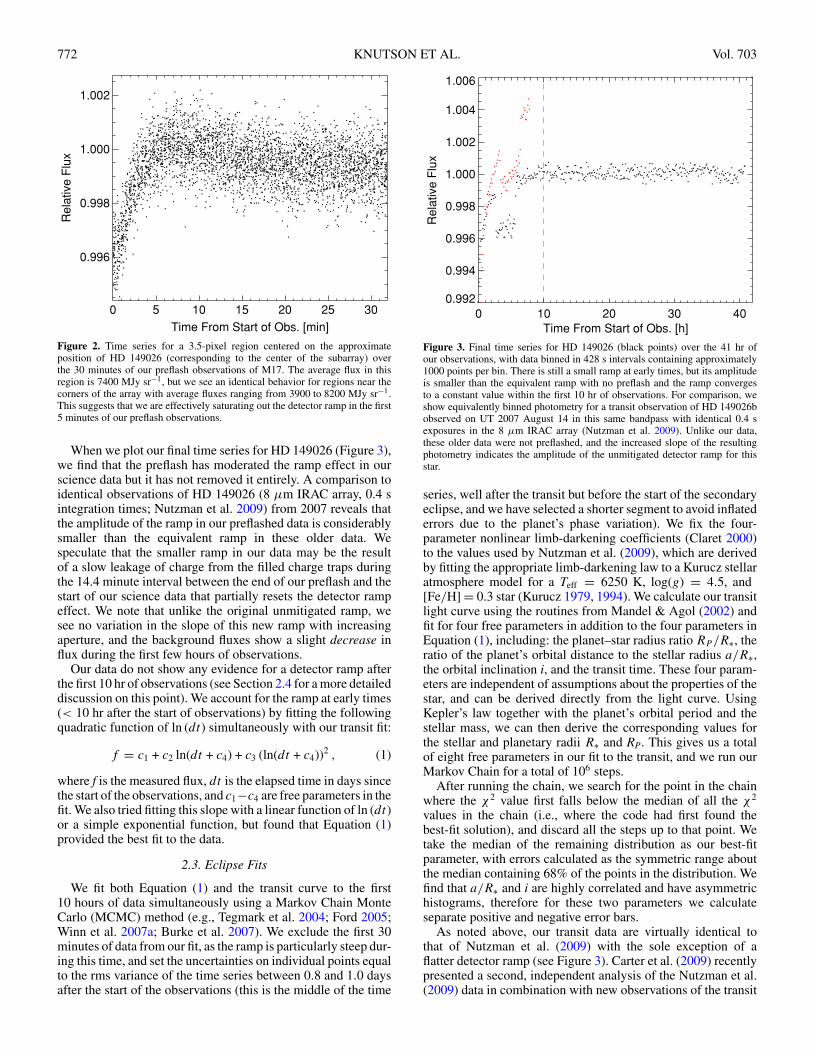
We evaluate the effectiveness of our preflash by calculatingthe total flux in an aperture with a 3.5-pixel radius centered on(1) the center of the array in the preflash images, correspondingto the position of HD 149026 in our science observations, (2) aregion near the corner of the array in the preflash images witha lower flux around 3500 MJy sr−1, and (3) a bright star inthe opposite corner of the array in the preflash images with apeak flux of 13,000 MJy sr−1. We find that in all cases thereis a linear increase in the measured flux during the first 5minutes of observations with a total amplitude of 0.4% (seeFigure 2), followed by a slight decrease in the measured fluxand then remaining effectively constant for the final 15 minutesof observations. Based on these data, we conclude that theeffectiveness of our preflash is independent of the brightness ofour preflash source above a minimum threshold value of 4000MJy sr−1, and that the charge traps across our entire 32 × 32pixel subarray are filled in the first 5 minutes of our preflashobservations.
772 KNUTSON ET AL. Vol. 703
0 5 10 15 20 25 30
Time From Start of Obs. [min]
0.996
0.998
1.000
1.002
Rela
tive F
lux
Figure 2. Time series for a 3.5-pixel region centered on the approximateposition of HD 149026 (corresponding to the center of the subarray) overthe 30 minutes of our preflash observations of M17. The average flux in thisregion is 7400 MJy sr−1, but we see an identical behavior for regions near thecorners of the array with average fluxes ranging from 3900 to 8200 MJy sr−1.This suggests that we are effectively saturating out the detector ramp in the first5 minutes of our preflash observations.
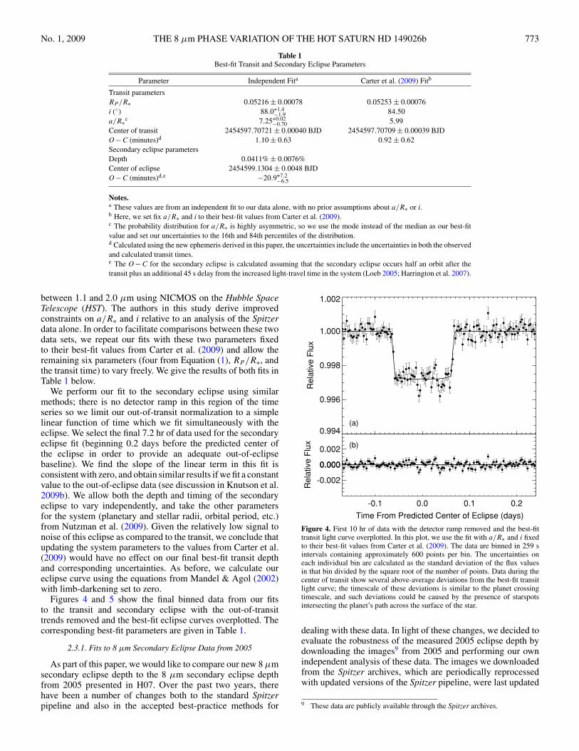
When we plot our final time series for HD 149026 (Figure 3),we find that the preflash has moderated the ramp effect in ourscience data but it has not removed it entirely. A comparison toidentical observations of HD 149026 (8 μm IRAC array, 0.4 sintegration times; Nutzman et al. 2009) from 2007 reveals thatthe amplitude of the ramp in our preflashed data is considerablysmaller than the equivalent ramp in these older data. Wespeculate that the smaller ramp in our data may be the resultof a slow leakage of charge from the filled charge traps duringthe 14.4 minute interval between the end of our preflash and thestart of our science data that partially resets the detector rampeffect. We note that unlike the original unmitigated ramp, wesee no variation in the slope of this new ramp with increasingaperture, and the background fluxes show a slight decrease influx during the first few hours of observations.
Our data do not show any evidence for a detector ramp afterthe first 10 hr of observations (see Section 2.4 for a more detaileddiscussion on this point). We account for the ramp at early times(< 10 hr after the start of observations) by fitting the followingquadratic function of ln (dt) simultaneously with our transit fit:
f = c1 + c2 ln(dt + c4) + c3 (ln(dt + c4))2 , (1)
where f is the measured flux, dt is the elapsed time in days sincethe start of the observations, and c1−c4 are free parameters in thefit. We also tried fitting this slope with a linear function of ln (dt)or a simple exponential function, but found that Equation (1)provided the best fit to the data.
2.3. Eclipse Fits
We fit both Equation (1) and the transit curve to the first10 hours of data simultaneously using a Markov Chain MonteCarlo (MCMC) method (e.g., Tegmark et al. 2004; Ford 2005;Winn et al. 2007a; Burke et al. 2007). We exclude the first 30minutes of data from our fit, as the ramp is particularly steep dur-ing this time, and set the uncertainties on individual points equalto the rms variance of the time series between 0.8 and 1.0 daysafter the start of the observations (this is the middle of the time
0 10 20 30 40Time From Start of Obs. [h]
0.992
0.994
0.996
0.998
1.000
1.002
1.004
1.006
Re
lativ
e F
lux
Figure 3. Final time series for HD 149026 (black points) over the 41 hr ofour observations, with data binned in 428 s intervals containing approximately1000 points per bin. There is still a small ramp at early times, but its amplitudeis smaller than the equivalent ramp with no preflash and the ramp convergesto a constant value within the first 10 hr of observations. For comparison, weshow equivalently binned photometry for a transit observation of HD 149026bobserved on UT 2007 August 14 in this same bandpass with identical 0.4 sexposures in the 8 μm IRAC array (Nutzman et al. 2009). Unlike our data,these older data were not preflashed, and the increased slope of the resultingphotometry indicates the amplitude of the unmitigated detector ramp for thisstar.
series, well after the transit but before the start of the secondaryeclipse, and we have selected a shorter segment to avoid inflatederrors due to the planet’s phase variation). We fix the four-parameter nonlinear limb-darkening coefficients (Claret 2000)to the values used by Nutzman et al. (2009), which are derivedby fitting the appropriate limb-darkening law to a Kurucz stellaratmosphere model for a Teff = 6250 K, log(g) = 4.5, and[Fe/H] = 0.3 star (Kurucz 1979, 1994). We calculate our transitlight curve using the routines from Mandel & Agol (2002) andfit for four free parameters in addition to the four parameters inEquation (1), including: the planet–star radius ratio RP /R∗, theratio of the planet’s orbital distance to the stellar radius a/R∗,the orbital inclination i, and the transit time. These four param-eters are independent of assumptions about the properties of thestar, and can be derived directly from the light curve. UsingKepler’s law together with the planet’s orbital period and thestellar mass, we can then derive the corresponding values forthe stellar and planetary radii R∗ and RP. This gives us a totalof eight free parameters in our fit to the transit, and we run ourMarkov Chain for a total of 106 steps.
After running the chain, we search for the point in the chainwhere the χ2 value first falls below the median of all the χ2
values in the chain (i.e., where the code had first found thebest-fit solution), and discard all the steps up to that point. Wetake the median of the remaining distribution as our best-fitparameter, with errors calculated as the symmetric range aboutthe median containing 68% of the points in the distribution. Wefind that a/R∗ and i are highly correlated and have asymmetrichistograms, therefore for these two parameters we calculateseparate positive and negative error bars.
As noted above, our transit data are virtually identical tothat of Nutzman et al. (2009) with the sole exception of aflatter detector ramp (see Figure 3). Carter et al. (2009) recentlypresented a second, independent analysis of the Nutzman et al.(2009) data in combination with new observations of the transit
No. 1, 2009 THE 8 μm PHASE VARIATION OF THE HOT SATURN HD 149026b 773
Table 1Best-fit Transit and Secondary Eclipse Parameters
Parameter Independent Fita Carter et al. (2009) Fitb
Transit parametersRP /R∗ 0.05216 ± 0.00078 0.05253 ± 0.00076i (◦) 88.0+1.4
−1.9 84.50a/R∗c 7.25+0.02
−0.70 5.99Center of transit 2454597.70721 ± 0.00040 BJD 2454597.70709 ± 0.00039 BJDO − C (minutes)d 1.10 ± 0.63 0.92 ± 0.62Secondary eclipse parametersDepth 0.0411% ± 0.0076%Center of eclipse 2454599.1304 ± 0.0048 BJDO − C (minutes)d,e −20.9+7.2
−6.5
Notes.a These values are from an independent fit to our data alone, with no prior assumptions about a/R∗ or i.b Here, we set fix a/R∗ and i to their best-fit values from Carter et al. (2009).c The probability distribution for a/R∗ is highly asymmetric, so we use the mode instead of the median as our best-fitvalue and set our uncertainties to the 16th and 84th percentiles of the distribution.d Calculated using the new ephemeris derived in this paper, the uncertainties include the uncertainties in both the observedand calculated transit times.e The O − C for the secondary eclipse is calculated assuming that the secondary eclipse occurs half an orbit after thetransit plus an additional 45 s delay from the increased light-travel time in the system (Loeb 2005; Harrington et al. 2007).
between 1.1 and 2.0 μm using NICMOS on the Hubble SpaceTelescope (HST). The authors in this study derive improvedconstraints on a/R∗ and i relative to an analysis of the Spitzerdata alone. In order to facilitate comparisons between these twodata sets, we repeat our fits with these two parameters fixedto their best-fit values from Carter et al. (2009) and allow theremaining six parameters (four from Equation (1), RP /R∗, andthe transit time) to vary freely. We give the results of both fits inTable 1 below.
We perform our fit to the secondary eclipse using similarmethods; there is no detector ramp in this region of the timeseries so we limit our out-of-transit normalization to a simplelinear function of time which we fit simultaneously with theeclipse. We select the final 7.2 hr of data used for the secondaryeclipse fit (beginning 0.2 days before the predicted center ofthe eclipse in order to provide an adequate out-of-eclipsebaseline). We find the slope of the linear term in this fit isconsistent with zero, and obtain similar results if we fit a constantvalue to the out-of-eclipse data (see discussion in Knutson et al.2009b). We allow both the depth and timing of the secondaryeclipse to vary independently, and take the other parametersfor the system (planetary and stellar radii, orbital period, etc.)from Nutzman et al. (2009). Given the relatively low signal tonoise of this eclipse as compared to the transit, we conclude thatupdating the system parameters to the values from Carter et al.(2009) would have no effect on our final best-fit transit depthand corresponding uncertainties. As before, we calculate oureclipse curve using the equations from Mandel & Agol (2002)with limb-darkening set to zero.
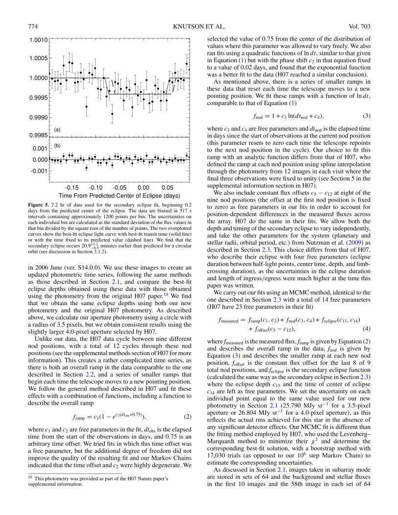
Figures 4 and 5 show the final binned data from our fitsto the transit and secondary eclipse with the out-of-transittrends removed and the best-fit eclipse curves overplotted. Thecorresponding best-fit parameters are given in Table 1.
2.3.1. Fits to 8 μm Secondary Eclipse Data from 2005
As part of this paper, we would like to compare our new 8 μmsecondary eclipse depth to the 8 μm secondary eclipse depthfrom 2005 presented in H07. Over the past two years, therehave been a number of changes both to the standard Spitzerpipeline and also in the accepted best-practice methods for
0.994
0.996
0.998
1.000
1.002
Re
lativ
e F
lux
(a)
(b)
-0.1 0.0 0.1 0.2
Time From Predicted Center of Eclipse (days)
-0.002
0.000
0.002
0.000
Re
lativ
e F
lux
Figure 4. First 10 hr of data with the detector ramp removed and the best-fittransit light curve overplotted. In this plot, we use the fit with a/R∗ and i fixedto their best-fit values from Carter et al. (2009). The data are binned in 259 sintervals containing approximately 600 points per bin. The uncertainties oneach individual bin are calculated as the standard deviation of the flux valuesin that bin divided by the square root of the number of points. Data during thecenter of transit show several above-average deviations from the best-fit transitlight curve; the timescale of these deviations is similar to the planet crossingtimescale, and such deviations could be caused by the presence of starspotsintersecting the planet’s path across the surface of the star.
dealing with these data. In light of these changes, we decided toevaluate the robustness of the measured 2005 eclipse depth bydownloading the images9 from 2005 and performing our ownindependent analysis of these data. The images we downloadedfrom the Spitzer archives, which are periodically reprocessedwith updated versions of the Spitzer pipeline, were last updated
9 These data are publicly available through the Spitzer archives.
774 KNUTSON ET AL. Vol. 703
0.9985
0.9990
0.9995
1.0000
1.0005
1.0010
(a)
(b)
-0.15 -0.10 -0.05 0.00 0.05
Time From Predicted Center of Eclipse (days)
-0.001
0.000
0.001
Figure 5. 7.2 hr of data used for the secondary eclipse fit, beginning 0.2days from the predicted center of the eclipse. The data are binned in 517 sintervals containing approximately 1200 points per bin. The uncertainties oneach individual bin are calculated as the standard deviation of the flux values inthat bin divided by the square root of the number of points. The two overplottedcurves show the best-fit eclipse light curve with best-fit transit time (solid line)or with the time fixed to its predicted value (dashed line). We find that thesecondary eclipse occurs 20.9+7.2
−6.5 minutes earlier than predicted for a circularorbit (see discussion in Section 3.1.2).
in 2006 June (ver. S14.0.0). We use these images to create anupdated photometric time series, following the same methodsas those described in Section 2.1, and compare the best-fiteclipse depths obtained using these data with those obtainedusing the photometry from the original H07 paper.10 We findthat we obtain the same eclipse depths using both our newphotometry and the original H07 photometry. As describedabove, we calculate our aperture photometry using a circle witha radius of 3.5 pixels, but we obtain consistent results using theslightly larger 4.0-pixel aperture selected by H07.
Unlike our data, the H07 data cycle between nine differentnod positions, with a total of 12 cycles through these nodpositions (see the supplemental methods section of H07 for moreinformation). This creates a rather complicated time series, asthere is both an overall ramp in the data comparable to the onedescribed in Section 2.2, and a series of smaller ramps thatbegin each time the telescope moves to a new pointing position.We follow the general method described in H07 and fit theseeffects with a combination of functions, including a function todescribe the overall ramp
framp = c1(1 − ec2(dtobs+0.75)), (2)
where c1 and c2 are free parameters in the fit, dtobs is the elapsedtime from the start of the observations in days, and 0.75 is anarbitrary time offset. We tried fits in which this time offset wasa free parameter, but the additional degree of freedom did notimprove the quality of the resulting fit and our Markov Chainsindicated that the time offset and c2 were highly degenerate. We
10 This photometry was provided as part of the H07 Nature paper’ssupplemental information.
selected the value of 0.75 from the center of the distribution ofvalues where this parameter was allowed to vary freely. We alsoran fits using a quadratic functions of ln dt , similar to that givenin Equation (1) but with the phase shift c2 in that equation fixedto a value of 0.02 days, and found that the exponential functionwas a better fit to the data (H07 reached a similar conclusion).
As mentioned above, there is a series of smaller ramps inthese data that reset each time the telescope moves to a newpointing position. We fit these ramps with a function of ln dt ,comparable to that of Equation (1)
fnod = 1 + c3 ln(dtnod + c4), (3)
where c3 and c4 are free parameters and dtnod is the elapsed timein days since the start of observations at the current nod position(this parameter resets to zero each time the telescope repointsto the next nod position in the cycle). Our choice to fit thisramp with an analytic function differs from that of H07, whodefined the ramp at each nod position using spline interpolationthrough the photometry from 12 images in each visit where thefinal three observations were fixed to unity (see Section 5 in thesupplemental information section in H07).
We also include constant flux offsets c5 − c12 at eight of thenine nod positions (the offset at the first nod position is fixedto zero) as free parameters in our fits in order to account forposition-dependent differences in the measured fluxes acrossthe array. H07 do the same in their fits. We allow both thedepth and timing of the secondary eclipse to vary independently,and take the other parameters for the system (planetary andstellar radii, orbital period, etc.) from Nutzman et al. (2009) asdescribed in Section 2.3. This choice differs from that of H07,who describe their eclipse with four free parameters (eclipseduration between half-light points, center time, depth, and limb-crossing duration), as the uncertainties in the eclipse durationand length of ingress/egress were much higher at the time thispaper was written.
We carry out our fits using an MCMC method, identical to theone described in Section 2.3 with a total of 14 free parameters(H07 have 23 free parameters in their fit)
fmeasured = framp(c1, c2) ∗ fnod(c3, c4) ∗ feclipse(c13, c14)
+ foffset(c5 − c12), (4)
where fmeasured is the measured flux, framp is given by Equation (2)and describes the overall ramp in the data, fnod is given byEquation (3) and describes the smaller ramp at each new nodposition, foffset is the constant flux offset for the last 8 of 9total nod positions, and feclipse is the secondary eclipse function(calculated the same way as the secondary eclipse in Section 2.3)where the eclipse depth c13 and the time of center of eclipsec14 are left as free parameters. We set the uncertainty on eachindividual point equal to the same value used for our newphotometry in Section 2.1 (25.790 MJy sr−1 for a 3.5-pixelaperture or 26.804 MJy sr−1 for a 4.0-pixel aperture), as thisreflects the actual rms achieved for this star in the absence ofany significant detector effects. Our MCMC fit is different thanthe fitting method employed by H07, who used the Levenberg–Marquardt method to minimize their χ2 and determine thecorresponding best-fit solution, with a bootstrap method with17,030 trials (as opposed to our 106 step Markov Chain) toestimate the corresponding uncertainties.
As discussed in Section 2.1, images taken in subarray modeare stored in sets of 64 and the background and stellar fluxesin the first 10 images and the 58th image in each set of 64
No. 1, 2009 THE 8 μm PHASE VARIATION OF THE HOT SATURN HD 149026b 775
have consistently lower values than the rest of the exposures.For our new data, we found that this effect was removed bythe background subtraction, but as a check we repeat ourfits to the updated photometry for the 2005 data with andwithout these images. We find that we obtain consistent eclipsedepths when we trim the 58th image alone (an eclipse depth of0.055% ± 0.007%), trim the first five images and 58th image(an eclipse depth of 0.057% ± 0.007%), or the first 10 imagesand the 58th image (an eclipse depth of 0.060% ± 0.008%). Ifwe change our method for removing transient hot pixels fromthe time series from the one described at the end of Section 2.1to a simple flux cutoff (any images with fluxes lower than 3000MJy sr−1 or higher than 3230 MJy sr−1 for a 3.5-pixel radiusaperture are removed, where the flux cutoffs are chosen usinga simple visual inspection of the time series), we obtain aneven deeper eclipse depth of 0.086%+0.016%
−0.020%. Using a 4.0-pixelaperture and our original bad pixel filtering method, and eithertrimming both the 58th image and first 10 images in each setof 64 or leaving those images in, we obtain eclipse depths of0.052% ± 0.009% and 0.048% ± 0.008%, respectively. If weallow the time offset of 0.75 in Equation (2) to vary freely inour fits with a 3.5-pixel aperture and trim the first 10 imagesand the 58th images, we obtain a slightly deeper eclipse depthwith larger uncertainties (0.076%+0.014%
−0.020%). However, this fit isnot stable, as we obtain a depth of 0.058%+0.009%
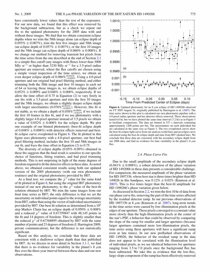
−0.012% if we includethe first 10 frames in this fit, and if we use photometry with aslightly larger 4.0-pixel aperture instead of 3.5 pixels we obtaina value of 0.052% ± 0.008% for the eclipse depth. We plotone example of our binned photometry (best-fit eclipse depthof 0.048% ± 0.008%) with detector effects removed and best-fit eclipse curve overplotted in Figure 6. The fit plotted in thisfigure uses photometry with a 4.0-pixel aperture, our best badpixel filtering method, includes the first 10 and 58th images inour fit, and fixes the time offset in Equation (2) to 0.75.
The diversity of eclipse depths (0.05%–0.09%) obtained inthese fits suggests that the final result is sensitive to our specificchoice of functions, fitting routines, and bad pixel trimmingmethods. This is not surprising in light of the many degrees offreedom required to fit the detector effects in these data. As notedabove, we obtained consistent results using both our updatedversion of the 2005 photometry (with our own photometryroutines) and the original photometry provided by H07.
As a final test, we compare the χ2 value for the same kindof fit plotted in Figure 6, but using the original H07 photometryinstead of our new photometry, to the χ2 value of the best-fitsolution obtained by H07. We trim the same images from ourfinal time series as H07; the only difference is that we set theuncertainty on individual points equal to the average uncertaintyfrom H07, rather than using the vector of individual uncertaintiesprovided by H07. Our best-fit solution as determined from a 106
step Markov Chain has an eclipse depth of 0.050% ± 0.008%and a reduced χ2 value of 0.67359847 with 48,145 points inthe fit and 14 degrees of freedom. This is slightly smaller thanthe reduced χ2 of 0.67368895 obtained by H07 with the samenumber of points and 23 degrees of freedom (J. Harrington 2009,private communication), but the difference is not statisticallysignificant.
Based on this analysis, we conclude that these data areconsistent with a shallower eclipse depth than that publishedby H07. As we discuss in more detail in Section 3.1.1, we findthat there is no evidence for variability in the planet’s 8 μmflux over the three-year interval between these data and our newobservations.
0.9985
0.9990
0.9995
1.0000
1.0005
1.0010
(a)
(b)
-0.15 -0.10 -0.05 0.00 0.05 0.10Time From Predicted Center of Eclipse (days)
-0.001
0.000
0.001
Figure 6. Updated photometry for an 8 μm eclipse of HD 149026b observedon UT 2005 August 24, originally published by Harrington et al. (2007). Thetime series shown in this plot is calculated our own photometry pipeline with a4.0-pixel radius aperture and has detector effects removed. These observationslasted 6.0 hr, but we have plotted the same time interval (7.2 hr) as in Figure 5to facilitate comparisons. The data are binned in 527 s intervals containingapproximately 1200 points per bin. The uncertainties on each individual binare calculated in the same way as Figure 5. The two overplotted curves showthe best-fit eclipse light curve from our analysis (solid line) and an eclipse curvecalculated using the best-fit eclipse depth and time from H07 (dashed line). Weconclude that these data are consistent with the secondary eclipse depth fromour 2008 data, and find no evidence for time variability in the planet’s 8 μmflux.
2.4. Phase Curve Fits
Due to the small amplitude of the secondary eclipse depth(0.041% ± 0.008%), a robust detection of the phase variationof HD 149206b in these data presents a considerable challenge.For comparison, the measured amplitude of the phase variationfor HD 189733b, whose host star is three times brighter than HD149026 in this bandpass, was 0.12% ± 0.02% (Knutson et al.2007). This is five times larger than the best-fit amplitude forHD 149026b’s phase variation given below.
As discussed in Section 2.2, we trim the first 10 hr of data fromour phase curve fits, removing the part of the time series affectedby the residual detector ramp. In our previous observations ofHD 189733b at 8 μm (Knutson et al. 2007), long-term trendsin the time series were caused by low-illumination pixels at theedges of our aperture. These pixels converged to a constant valuemore slowly than the high-illumination pixels at the center ofthe star’s PSF, a behavior that could be observed by comparingthe slope of the ramp for smaller and larger apertures (becauselarger apertures contained more low-illumination pixels, thetime series using these apertures will have a significant rampeven at late times). In our new preflashed observations ofHD 149026, the behavior of the residual ramp in the datadoes not appear to be correlated with the illumination levelof individual pixels, as we see identical behaviors for aperturesranging from 3.5 to 7.0 pixels once the background flux hasbeen subtracted. We take this as evidence that the low-flux,large-slope component of the ramp has been effectively removed
776 KNUTSON ET AL. Vol. 703
-0.1 0.0 0.1 0.2 0.3 0.4 0.5 0.6
Orbital Phase
0.9998
1.0000
1.0002
1.0004
1.0006
1.0008
Rel
ativ
e F
lux
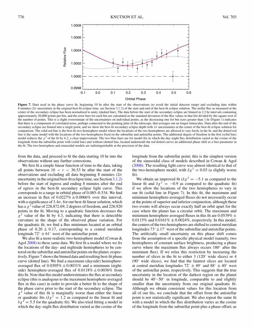
Figure 7. Data used in the phase curve fit, beginning 10 hr after the start of the observations (to avoid the initial detector ramp) and excluding data within8 minutes (2σ uncertainty in the original best-fit eclipse time, see Section 3.1.2) of the start and end of the best-fit eclipse solution. The stellar flux as measured at thecenter of the secondary eclipse has been normalized to unity (dashed line). The data before the start of the secondary eclipse are binned in 2.2 hr intervals containingapproximately 20,000 points per bin, and the error bars for each bin are calculated as the standard deviation of the flux values in that bin divided by the square root ofthe number of points. This is a slight overestimate of the uncertainties on individual points, as the decreasing rms for bin sizes greater than 1 hr (Figure 1) indicatesthat there is a component of correlated noise, perhaps connected to the pointing jitter of the telescope, that averages out on longer timescales. Data after the end of thesecondary eclipse are binned into a single point, and we show the best-fit secondary eclipse depth with 1σ uncertainties at the center of the best-fit eclipse solution forcomparison. The solid red line is the best-fit two-hemisphere model where the locations of the two hemispheres are allowed to vary freely in the fit, and the dotted redline is the same model with the locations of the two hemispheres fixed on the substellar and antistellar points. The additional degree of freedom in the first (solid line)model reduces the χ2 of the fit by 6.2, a clear improvement. The two blue lines are for model fits in which the day–night flux distribution varied as the cosine of thelongitude from the substellar point with (solid line) and without (dotted line, located underneath the red dotted curve) an additional phase shift as a free parameter inthe fit. The two-hemisphere and sinusoidal models are indistinguishable at the precision of the data.
from the data, and proceed to fit the data starting 10 hr into theobservations without any further corrections.
We first fit a simple linear function of time to the data, takingall points between 10 < t < 36.53 hr after the start of theobservations and excluding all data beginning 8 minutes (2σuncertainty in the original best-fit eclipse time, see Section 3.1.2)before the start of ingress and ending 8 minutes after the endof egress in the best-fit secondary eclipse light curve. Thiscorresponds to a range in orbital phase of 0.085–0.534. We findan increase in flux of 0.0227% ± 0.0066% over this interval,with a significance of 3.4σ , for our best-fit linear solution, whichhas a χ2 value of 228,872.69, 2 degrees of freedom, and 228,920points in the fit. Moving to a quadratic function decreases theχ2 value of the fit by 4.3, indicating that there is detectiblecurvature in the shape of the observed phase variation. Forthe quadratic fit, we find a flux minimum located at an orbitalphase of 0.20 ± 0.17, corresponding to a central meridianlongitude 72◦ ± 61◦ west of the antistellar point.
We also fit a more realistic two-hemisphere model (Cowan &Agol 2008) to these same data. We first fit a model where we fixthe locations of the day- and nightside hemispheres to be cen-tered on the substellar and antistellar points on the planet, respec-tively. Figure 7 shows the binned data and resulting best-fit phasecurve (dotted line). We find a maximum (dayside) hemisphere-averaged flux of 0.0305% ± 0.0031% and a minimum (night-side) hemisphere-averaged flux of 0.0118% ± 0.0036% fromthis fit. Note that this model underestimates the flux at secondaryeclipse (this is analogous to the maximum hemisphere-averagedflux in this case) in order to provide a better fit to the shape ofthe phase curve prior to the start of the secondary eclipse. Theχ2 value of this fit is marginally worse than either the linearor quadratic fits (δχ2 = 1.2 as compared to the linear fit andδχ2 = 5.5 for the quadratic fit). We also tried fitting a model inwhich the day–night flux distribution varied as the cosine of the
longitude from the substellar point; this is the simplest versionof the sinusoidal class of models described in Cowan & Agol(2008). The resulting light curve was almost identical to that ofthe two-hemisphere model, with δχ2 = 0.03 (a slightly worsefit).
We obtain an improved fit (δχ2 = −5.1 as compared to thelinear fit and δχ2 = −0.9 as compared to the quadratic fit)if we allow the locations of the two hemispheres to vary inour fit (solid line in Figure 7). In this fit, the maximum andminimum hemisphere-averaged fluxes do not necessarily occurat the points of superior and inferior conjunction, although thesetwo events will always occur exactly half an orbit apart for thecase where the planet has a circular orbit. The maximum andminimum hemisphere-averaged fluxes in this fit are 0.0539% ±0.0115% and 0.0161% ± 0.0024%, respectively. In this model,the centers of the two hemispheres are shifted to central meridianlongitudes 73◦±17◦ west of the substellar and antistellar points.The artificially small uncertainty on this phase shift comesfrom the assumption of a specific physical model (namely, twohemispheres of constant surface brightness, producing a phasecurve where the maximum flux always occurs 180◦ after theminimum flux). If we relax this restriction by increasing thenumber of slices in the fit to either 3 (120◦ wide slices) or 4(90◦ wide slices), we find that the faintest slices are locatedat central meridian longitudes 72◦ ± 49◦ and 88◦ ± 40◦ westof the antistellar point, respectively. This suggests that the trueuncertainty in the location of the darkest region on the planetshould be 40◦–50◦ in longitude, comparable to and slightlysmaller than the uncertainty from our original quadratic fit.Although we obtain consistent values for this location fromall of our fits, we conclude that the offset from the antistellarpoint is not statistically significant. We also repeat the same fitwith a model in which the flux distribution varies as the cosineof the longitude from the substellar point plus a phase offset; as
No. 1, 2009 THE 8 μm PHASE VARIATION OF THE HOT SATURN HD 149026b 777
-5 0 5Time From Transit Center [d]
0.996
0.998
1.000
1.002
1.004
Rela
tive F
lux
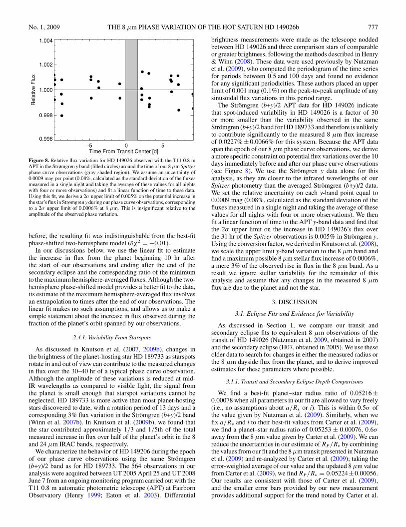
Figure 8. Relative flux variation for HD 149026 observed with the T11 0.8 mAPT in the Strømgren y band (filled circles) around the time of our 8 μm Spitzerphase curve observations (gray shaded region). We assume an uncertainty of0.0009 mag per point (0.08%, calculated as the standard deviation of the fluxesmeasured in a single night and taking the average of these values for all nightswith four or more observations) and fit a linear function of time to these data.Using this fit, we derive a 2σ upper limit of 0.005% on the potential increase inthe star’s flux in Strømgren y during our phase curve observations, correspondingto a 2σ upper limit of 0.0006% at 8 μm. This is insignificant relative to theamplitude of the observed phase variation.
before, the resulting fit was indistinguishable from the best-fitphase-shifted two-hemisphere model (δχ2 = −0.01).
In our discussions below, we use the linear fit to estimatethe increase in flux from the planet beginning 10 hr afterthe start of our observations and ending after the end of thesecondary eclipse and the corresponding ratio of the minimumto the maximum hemisphere-averaged fluxes. Although the two-hemisphere phase-shifted model provides a better fit to the data,its estimate of the maximum hemisphere-averaged flux involvesan extrapolation to times after the end of our observations. Thelinear fit makes no such assumptions, and allows us to make asimple statement about the increase in flux observed during thefraction of the planet’s orbit spanned by our observations.
2.4.1. Variability From Starspots
As discussed in Knutson et al. (2007, 2009b), changes inthe brightness of the planet-hosting star HD 189733 as starspotsrotate in and out of view can contribute to the measured changesin flux over the 30–40 hr of a typical phase curve observation.Although the amplitude of these variations is reduced at mid-IR wavelengths as compared to visible light, the signal fromthe planet is small enough that starspot variations cannot beneglected. HD 189733 is more active than most planet-hostingstars discovered to date, with a rotation period of 13 days and acorresponding 3% flux variation in the Stromgren (b+y)/2 band(Winn et al. 2007b). In Knutson et al. (2009b), we found thatthe star contributed approximately 1/3 and 1/5th of the totalmeasured increase in flux over half of the planet’s orbit in the 8and 24 μm IRAC bands, respectively.
We characterize the behavior of HD 149206 during the epochof our phase curve observations using the same Stromgren(b+y)/2 band as for HD 189733. The 564 observations in ouranalysis were acquired between UT 2005 April 25 and UT 2008June 7 from an ongoing monitoring program carried out with theT11 0.8 m automatic photometric telescope (APT) at FairbornObservatory (Henry 1999; Eaton et al. 2003). Differential
brightness measurements were made as the telescope noddedbetween HD 149026 and three comparison stars of comparableor greater brightness, following the methods described in Henry& Winn (2008). These data were used previously by Nutzmanet al. (2009), who computed the periodogram of the time seriesfor periods between 0.5 and 100 days and found no evidencefor any significant periodicities. These authors placed an upperlimit of 0.001 mag (0.1%) on the peak-to-peak amplitude of anysinusoidal flux variations in this period range.
The Stromgren (b+y)/2 APT data for HD 149026 indicatethat spot-induced variability in HD 149026 is a factor of 30or more smaller than the variability observed in the sameStromgren (b+y)/2 band for HD 189733 and therefore is unlikelyto contribute significantly to the measured 8 μm flux increaseof 0.0227% ± 0.0066% for this system. Because the APT dataspan the epoch of our 8 μm phase curve observations, we derivea more specific constraint on potential flux variations over the 10days immediately before and after our phase curve observations(see Figure 8). We use the Stromgren y data alone for thisanalysis, as they are closer to the infrared wavelengths of ourSpitzer photometry than the averaged Stromgren (b+y)/2 data.We set the relative uncertainty on each y-band point equal to0.0009 mag (0.08%, calculated as the standard deviation of thefluxes measured in a single night and taking the average of thesevalues for all nights with four or more observations). We thenfit a linear function of time to the APT y-band data and find thatthe 2σ upper limit on the increase in HD 149026’s flux overthe 31 hr of the Spitzer observations is 0.005% in Stromgren y.Using the conversion factor, we derived in Knutson et al. (2008),we scale the upper limit y-band variation to the 8 μm band andfind a maximum possible 8 μm stellar flux increase of 0.0006%,a mere 3% of the observed rise in flux in the 8 μm band. As aresult we ignore stellar variability for the remainder of thisanalysis and assume that any changes in the measured 8 μmflux are due to the planet and not the star.
3. DISCUSSION
3.1. Eclipse Fits and Evidence for Variability
As discussed in Section 1, we compare our transit andsecondary eclipse fits to equivalent 8 μm observations of thetransit of HD 149026 (Nutzman et al. 2009, obtained in 2007)and the secondary eclipse (H07, obtained in 2005). We use theseolder data to search for changes in either the measured radius orthe 8 μm dayside flux from the planet, and to derive improvedestimates for these parameters where possible.
3.1.1. Transit and Secondary Eclipse Depth Comparisons
We find a best-fit planet–star radius ratio of 0.05216 ±0.00078 when all parameters in our fit are allowed to vary freely(i.e., no assumptions about a/R∗ or i). This is within 0.5σ ofthe value given by Nutzman et al. (2009). Similarly, when wefix a/R∗ and i to their best-fit values from Carter et al. (2009),we find a planet–star radius ratio of 0.05253 ± 0.00076, 0.6σaway from the 8 μm value given by Carter et al. (2009). We canreduce the uncertainties in our estimate of RP /R∗ by combiningthe values from our fit and the 8 μm transit presented in Nutzmanet al. (2009) and re-analyzed by Carter et al. (2009); taking theerror-weighted average of our value and the updated 8 μm valuefrom Carter et al. (2009), we find RP /R∗ = 0.05224±0.00056.Our results are consistent with those of Carter et al. (2009),and the smaller error bars provided by our new measurementprovides additional support for the trend noted by Carter et al.
778 KNUTSON ET AL. Vol. 703
(2009), in which the transit depth between 1 and 2 μm appears tobe marginally deeper than the equivalent values for visible-lightphotometry (Winn et al. 2008) and the Spitzer 8 μm bandpass.Carter et al. (2009) conclude that this discrepancy is most likelydue to systematic errors rather than a real variation in theproperties of the planet’s atmosphere; the noise in their 1.4 μmNICMOS data is a factor of 2 above the predicted photon noiseand its properties are poorly understood. The good agreementbetween our 8 μm transit and that of Nutzman et al. (2009)suggests that the problem most likely lies with the NICMOSdata, as the noise in the Spitzer data sets is only a factor of 1.28and 1.15 above the photon noise limit, respectively.
If we compare our new secondary eclipse depth to thatreported by H07 in this bandpass, it initially appears as if thisquantity might be varying in time. Our best-fit secondary eclipsedepth is 0.0411% ± 0.0076%, a factor of 2 smaller (3.0σ )than the value of 0.082%+0.009%
−0.012% from H07. Fixing the timeof secondary eclipse in our fits to its predicted value results ina slightly shallower eclipse depth, with a net change of 0.006%or 0.8σ as compared to our original fit.
It is possible that the removal of large-amplitude detectoreffects in the older H07 data might have resulted in an over-estimate of the true eclipse depth, in which case our two mea-surements might in fact be consistent. Although, H07 used thesame 0.4 s exposure time and 8 μm IRAC subarray as we did,our observations place the star at a single pixel at the center ofthe subarray whereas the H07 data cycle between nine differentnod positions, with a total of 12 complete cycles over 6.4 hr ofobservations. Each nod position has a slightly different gain andthe move to a new nod position results in a slight reset of the de-tector ramp effect described in Section 2.2, therefore H07 mustfit a total of 23 free parameters in their fit as compared to ourfour free parameters. They must also remove a ramp spanningthe entire data set with a total rise of 1.3%, 15 times larger thantheir inferred 0.084% decrease in flux during secondary eclipse.
As compared to the H07 fits, our analysis is much simpler. Wedo not nod, therefore we have no need to normalize to differentnod positions. We preflash our data to mitigate the ramp andthe secondary eclipse occurs at the end of our observations,where the slope is minimal (the best-fit coefficient for the linearfunction of time in our eclipse fits differs from zero by only0.2σ and we obtain the same results when we limit our fits toa simple constant term to describe the out-of-eclipse flux). Wealso have more data out of eclipse than H07, which is helpfulfor determining a robust out-of-eclipse baseline. Although theuncertainties in our measured eclipse depth are only slightlysmaller than those reported by H07 for the 2005 eclipse, weconclude that our new eclipse depth is a more reliable estimateof the planet’s 8 μm flux for the reasons listed above.
As discussed in Section 2.3.1, we evaluate the robustness ofthe eclipse depth provided by H07 by downloading the imagesfrom 2005 from the Spitzer archives and performing our ownindependent analysis of these data. Depending on our specificchoices for which data to trim and what functional forms to fit,we find eclipse depths ranging from 0.05% to 0.08%, althoughan eclipse depth around 0.05% is preferred in a majority of ourfits (Figure 6). If we repeat these fits using the same photometryas H07, we find solutions with eclipse depths closer to 0.05%where the χ2 value is indistinguishable from the best χ2 valueobtained by H07. Our results suggest that the 2005 data are infact consistent with our new 2008 observations, and we thereforeconclude that there is no evidence for variability in the planet’s8 μm flux.
-400 -300 -200 -100 0 100
Orbit Number
-20
-15
-10
-5
0
5
10
15
O-C
(m
in)
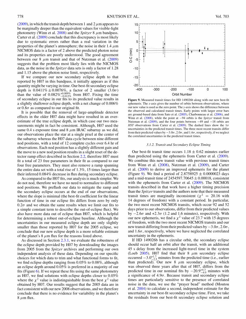
Figure 9. Measured transit times for HD 149026b along with our new best-fitephemeris. The x-axis gives the number of orbits between observations, whereour new value is used as the zero point. The y-axis shows the difference betweenthe observed and calculated transit times. Early points with larger error barsare ground-based data from Sato et al. (2005), Charbonneau et al. (2006), andWinn et al. (2008), while the point at −94 orbits is the Spitzer transit fromNutzman et al. (2009), and the four points between −49 and −18 orbits areHST observations from Carter et al. (2009). The dashed lines show the 1σ
uncertainties in the predicted transit times. The three most recent transits differfrom their predicted values by −3.0σ , 2.0σ , and 1.6σ , respectively, if we neglectthe correlated uncertainties in the predicted transit times.
3.1.2. Transit and Secondary Eclipse Timing
Our best-fit transit time occurs 1.18 ± 0.62 minutes earlierthan predicted using the ephemeris from Carter et al. (2009).We combine this new transit value with previous transit timesfrom Winn et al. (2008), Nutzman et al. (2009), and Carteret al. (2009) to derive an improved ephemeris for the planet(Figure 9). We find a period of 2.8758925 ± 0.0000023 daysand a mid-transit time of 2454597.70645 ± 0.00018, consistentwith the ephemeris from Carter et al. (2009). The NICMOStransits described in that work have a higher timing precisionthan the Spitzer transits and the authors note that their measuredtransit times are marginally inconsistent (χ2 = 20.16 with14 degrees of freedom) with a constant period. In particular,the two most recent NICMOS transits, which occur 92 and 52days prior to our observations, differ from their predicted valuesby −2.6σ and +2.3σ (1.2 and 1.6 minutes), respectively. Withour new ephemeris, we find a χ2 value of 23.7 with 15 degreesof freedom, with the two most recent NICMOS transits and ournew transit differing from their predicted values by −3.0σ , 2.0σ ,and 1.6σ , respectively, where we have neglected the correlateduncertainty in the ephemeris.
If HD 149026b has a circular orbit, the secondary eclipseshould occur half an orbit after the transit, with an additional45 s delay from the increased light-travel time in the system(Loeb 2005). H07 find that their 8 μm secondary eclipseoccurred −3.0+1.7
−2.5 minutes from the predicted time (i.e., earlierthan predicted). Our new 8 μm secondary eclipse, whichwas observed three years after that of H07, differs from thepredicted time in our nominal fits by −20.9+4.3
−4.0 minutes witha significance of 4.9σ . Because transit and secondary eclipsetimes are particularly sensitive to the presence of correlatednoise in the data, we use the “prayer bead” method (Moutouet al. 2004) to calculate a second, independent estimate for theuncertainty in our best-fit secondary eclipse time. First, we takethe residuals from our best-fit secondary eclipse solution and
No. 1, 2009 THE 8 μm PHASE VARIATION OF THE HOT SATURN HD 149026b 779
-40 -30 -20 -10 0 10Offset in Eclipse Time [min]
0.01
0.02
0.03
0.04
Pro
ba
bili
ty D
en
sity
-40 -30 -20 -10 0 10Offset in Eclipse Time [min]
0.00
0.01
0.02
0.03
0.04
0.05
0.06
Pro
ba
bili
ty D
en
sity
-40 -30 -20 -10 0 10Offset in Eclipse Time [min]
0.01
0.02
0.03
0.04
Pro
ba
bili
ty D
en
sity
-40 -30 -20 -10 0 10Offset in Eclipse Time [min]
0.00
0.01
0.02
0.03
0.04
0.05
Pro
ba
bili
ty D
en
sity
-40 -30 -20 -10 0 10Offset in Eclipse Time [min]
0.00
0.01
0.02
0.03
0.04
0.05
Pro
ba
bili
ty D
en
sity
-40 -30 -20 -10 0 10Offset in Eclipse Time [min]
0.00
0.01
0.02
0.03
0.04
0.05
0.06P
rob
ab
ility
De
nsi
ty
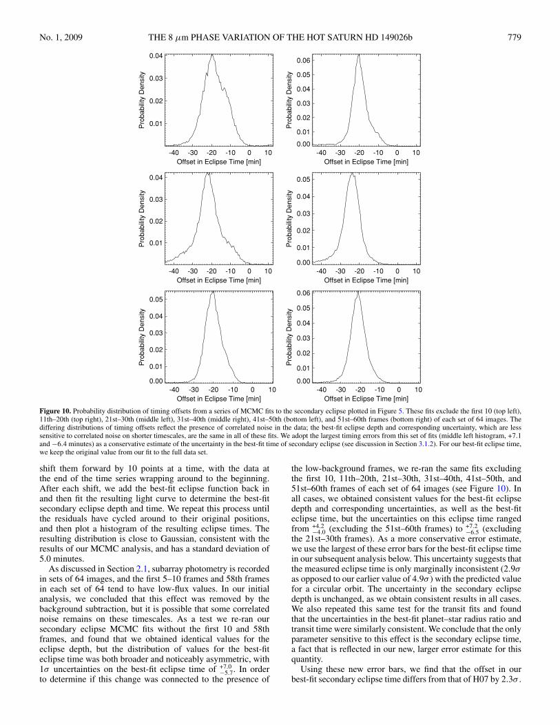
Figure 10. Probability distribution of timing offsets from a series of MCMC fits to the secondary eclipse plotted in Figure 5. These fits exclude the first 10 (top left),11th–20th (top right), 21st–30th (middle left), 31st–40th (middle right), 41st–50th (bottom left), and 51st–60th frames (bottom right) of each set of 64 images. Thediffering distributions of timing offsets reflect the presence of correlated noise in the data; the best-fit eclipse depth and corresponding uncertainty, which are lesssensitive to correlated noise on shorter timescales, are the same in all of these fits. We adopt the largest timing errors from this set of fits (middle left histogram, +7.1and −6.4 minutes) as a conservative estimate of the uncertainty in the best-fit time of secondary eclipse (see discussion in Section 3.1.2). For our best-fit eclipse time,we keep the original value from our fit to the full data set.
shift them forward by 10 points at a time, with the data atthe end of the time series wrapping around to the beginning.After each shift, we add the best-fit eclipse function back inand then fit the resulting light curve to determine the best-fitsecondary eclipse depth and time. We repeat this process untilthe residuals have cycled around to their original positions,and then plot a histogram of the resulting eclipse times. Theresulting distribution is close to Gaussian, consistent with theresults of our MCMC analysis, and has a standard deviation of5.0 minutes.
As discussed in Section 2.1, subarray photometry is recordedin sets of 64 images, and the first 5–10 frames and 58th framesin each set of 64 tend to have low-flux values. In our initialanalysis, we concluded that this effect was removed by thebackground subtraction, but it is possible that some correlatednoise remains on these timescales. As a test we re-ran oursecondary eclipse MCMC fits without the first 10 and 58thframes, and found that we obtained identical values for theeclipse depth, but the distribution of values for the best-fiteclipse time was both broader and noticeably asymmetric, with1σ uncertainties on the best-fit eclipse time of +7.0
−5.7. In orderto determine if this change was connected to the presence of
the low-background frames, we re-ran the same fits excludingthe first 10, 11th–20th, 21st–30th, 31st–40th, 41st–50th, and51st–60th frames of each set of 64 images (see Figure 10). Inall cases, we obtained consistent values for the best-fit eclipsedepth and corresponding uncertainties, as well as the best-fiteclipse time, but the uncertainties on this eclipse time rangedfrom +4.2
−4.0 (excluding the 51st–60th frames) to +7.2−6.5 (excluding
the 21st–30th frames). As a more conservative error estimate,we use the largest of these error bars for the best-fit eclipse timein our subsequent analysis below. This uncertainty suggests thatthe measured eclipse time is only marginally inconsistent (2.9σas opposed to our earlier value of 4.9σ ) with the predicted valuefor a circular orbit. The uncertainty in the secondary eclipsedepth is unchanged, as we obtain consistent results in all cases.We also repeated this same test for the transit fits and foundthat the uncertainties in the best-fit planet–star radius ratio andtransit time were similarly consistent. We conclude that the onlyparameter sensitive to this effect is the secondary eclipse time,a fact that is reflected in our new, larger error estimate for thisquantity.
Using these new error bars, we find that the offset in ourbest-fit secondary eclipse time differs from that of H07 by 2.3σ .
780 KNUTSON ET AL. Vol. 703
In our re-analysis of the H07 data (Section 3.1.1), we find abest-fit eclipse time 3.3 minutes later than the value derived byH07, albeit with larger uncertainties (±3.5 minutes as opposedto H07’s value of +1.7
−2.5 minutes). Using this value, the timingoffset in the 2005 eclipse differs from that of our 2008 eclipseby 2.6σ . If this offset is confirmed by future observations, itwould suggest that the planet’s orbit may have changed duringthe three-year interval between the two observations.
The timing offset observed in our new data corresponds toa value of −0.0079+0.0027
−0.0025 for e cos (ω), where e is the planet’sorbital eccentricity and ω is the argument of pericenter. This isconsistent with the radial velocity observations of this systemfrom Sato et al. (2005) and Wolf et al. (2007), which arepoorly sampled and thus do not provide strong constraintson the planet’s orbital eccentricity. Madhusudhan & Winn(2009) derive upper limits on e sin (ω) and e cos (ω) from asimultaneous fit to the available transit, secondary eclipse, andradial velocity data, but the uncertainty in e cos (ω) is dominatedby the uncertainty in the secondary eclipse time from H07 andtheir value for e sin (ω) = 0.109+0.042
−0.068 is still poorly constrainedrelative to our estimate for e cos (ω). If real, the observedchange in e cos (ω) could be due to either a changing orbitaleccentricity or a precessing orbit (i.e., a change in e or in ω).The addition of four new secondary eclipses observed as part ofan ongoing Spitzer target of opportunity program (J. Harrington2009, private communication) should either confirm or disprovethe presence of the timing offset suggested by our data, as wellas constraining any temporal variability in this quantity.
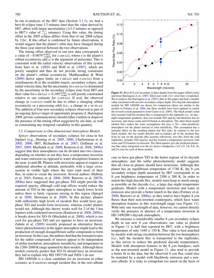
3.2. Comparisons to One-dimensional Atmosphere ModelsSpitzer observations of secondary eclipses for close-in hot
Jupiters (e.g., Deming et al. 2005, 2006; Charbonneau et al.2005, 2008; H07; Richardson et al. 2007; Grillmair et al.2007, 2009; Machalek et al. 2008; Knutson et al. 2008, 2009a)suggest that their atmospheres can be divided into two classes,depending on whether or not they have a temperature inversionand water emission (as opposed to water absorption) features inthe near- to mid-IR. Planets with inversions appear to require anadditional absorber at altitude, preferably with a large cross-section in visible light where the stars emit most of theirflux, in order to create the inversion. Several authors (Hubenyet al. 2003; Fortney et al. 2006, 2008; Burrows et al. 2007b,2008a) have suggested that gas-phase TiO might provide therequired opacity, although cold trap effects would reduce theamount of TiO in the upper atmosphere to much lower levelsunless there is fairly vigorous mixing in this region (Spiegelet al. 2009; Showman et al. 2009). In this picture, planetswith sufficiently high levels of incident flux would have gas-phase TiO and would form inversions, whereas cooler planetswould not. Although this theory works well for 2 of the 3 hotJupiters with confirmed inversions (Knutson et al. 2008, 2009a),it breaks down for XO-1b (Machalek et al. 2008), which is toocool for gas-phase TiO and yet appears to have an inversion.Zahnle et al. (2009) recently proposed an alternative theorywhere photochemistry in the upper atmosphere might lead to theproduction of enough disequilibrium sulfur compounds to forman inversion. In this case, the authors find that the formation ratesfor the sulfur compounds of interest appear to be independentof stellar insolation, atmospheric metallicity, and temperature inthe 1200–2000 K range spanned by their models. Although thesemodels correctly predict that XO-1b should have an inversion,they fail to explain why HD 189733b and TrES-1 do not.
HD 149026b is a clear candidate for an inversion in eitherscenario, as it receives enough incident flux in the zero-albedo
2 3 4 5 6 7 8 9 10 20
Wavelength (microns)
0.00
0.02
0.04
0.06
0.08
0.10
0.12
Pla
net-
Sta
r F
lux
Ratio
(%
)
Figure 11. Best-fit 8 μm secondary eclipse depths from this paper (filled circle)and from Harrington et al. (2007; filled star) with ±1σ error bars overplotted.We re-analyze the Harrington et al. (2007) data in this paper and find a smallervalue consistent with our new secondary eclipse depth. Two dayside atmospheremodels for HD 149026b are shown for comparison (these are similar to themodels in Fortney et al. 2006, but these models have been updated to matchthe revised system parameters from Carter et al. 2009). The black model (solidline) assumes half the incident flux is transported to the nightside (i.e., no day–night temperature gradient), does not include TiO opacity and therefore has noinversion, and shows water and CO bands in absorption. The other black model(dotted line) makes the same assumptions but uses a 30× solar-metallicityatmosphere for the planet instead of solar metallicity. This assumption has aminimal effect on the resulting planet–star flux ratio. In contrast to the twoblack models, the red model absorbs and re-radiates all of the incident fluxfrom its star on the dayside (this assumes effectively zero flux from the coldnightside), includes TiO opacity, and has formed a temperature inversion withwater and CO features in emission. The filled squares give the predicted planet–star flux ratios integrated over the six Spitzer bandpasses (3.6, 4.5, 5.8, 8.0, 16,and 24 μm) for each of these models.
case to have gas-phase TiO in the hotter regions of its daysideatmosphere, and the sulfur photochemistry model suggeststhat all close-in planets should have inversions. Although thisplanet has an equilibrium temperature of 1740 K, the 8 μmsecondary eclipse depth measured by H07 corresponds to an8 μm brightness temperature of 2300 ± 200 K. In order tomatch this high dayside flux, models must keep as much energyas possible on the dayside (i.e., a large day–night temperaturegradient). Models with a temperature inversion and water inemission also provide a better match to the data (Fortney et al.2006; Burrows et al. 2008a), as they tend to have higher 8 μmfluxes than their non-inverted counterparts, which have waterabsorption features in this wavelength range (see Figure 11).With only one wavelength of data, however, we cannot directlyverify the presence or absence of a temperature inversion inHD 149026b’s dayside atmosphere.
We measure a considerably smaller 8 μm secondary eclipsedepth in our new 8 μm observations; our value as plottedin Figure 11 is half that reported by H07, with a brightnesstemperature of only 1440 ± 150 K. This value is best matchedby models with strong circulation between the two hemispheres(i.e., half the incident flux is transported to the nightside),as this serves to reduce the predicted dayside temperatures.Models with absorption features in the 8 μm bandpass, suchas the non-inverted model in Figure 11, also tend to providea better fit to the data, but the observed 8 μm flux could alsobe matched by a model with blackbody emission and a non-zero albedo. It is risky to extrapolate too much on the basis of
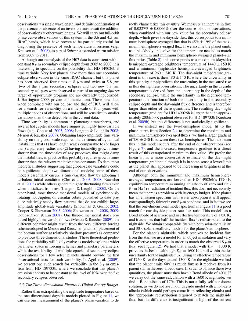
No. 1, 2009 THE 8 μm PHASE VARIATION OF THE HOT SATURN HD 149026b 781
observations at a single wavelength, and definite confirmation ofthe presence or absence of an inversion must await the additionof observations at other wavelengths. We will carry out full-orbitphase curve observations of this system in the 3.6 and 4.5 μmIRAC bands, which have proven to be particularly useful fordiagnosing the presence of such temperature inversions (e.g.,Knutson et al. 2008), as part of Spitzer’s extended warm missionfrom 2009 to 2011.
Although our reanalysis of the H07 data is consistent with aconstant 8 μm secondary eclipse depth from 2005 to 2008, it isinteresting to speculate on the possibility that HD 149026b istime variable. Very few planets have more than one secondaryeclipse observation in the same IRAC channel, but this planethas been observed four times at 8 μm and twice at 5.8 μm(two of the 8 μm secondary eclipses and two new 5.8 μmsecondary eclipses were observed as part of an ongoing Spitzertarget of opportunity program and are currently unpublished;J. Harrington 2009, private communication). These new data,when combined with our eclipse and that of H07, will allowfor a search for variability on a time scale of four years withmultiple epochs of observations, and will be sensitive to smallervariations than those detectible in the current data.
Time variability is common in planetary atmospheres, andseveral hot Jupiter models have suggested highly time-variableflows (e.g., Cho et al. 2003, 2008; Langton & Laughlin 2008;Menou & Rausher 2009). Obtaining large-amplitude time vari-ability on the global scale requires the existence of dynamicalinstabilities that (1) have length scales comparable to (or largerthan) a planetary radius and (2) having instability growth timesshorter than the timescales of any processes that might dampthe instabilities; in practice this probably requires growth timesshorter than the relevant radiative time constants. To date, mosttheoretical studies suggesting that global-scale variability couldbe significant adopt two-dimensional models; some of thesemodels essentially ensure a time-variable flow by adopting aturbulent initial condition (Cho et al. 2003, 2008; Rauscheret al. 2008) while others generate highly fluctuating flows evenwhen initialized from rest (Langton & Laughlin 2008). On theother hand, most three-dimensional models of synchronouslyrotating hot Jupiters on circular orbits published to date pro-duce relatively steady flow patterns that do not exhibit large-amplitude global-scale variability (Showman & Guillot 2002;Cooper & Showman 2005, 2006; Showman et al. 2008, 2009;Dobbs-Dixon & Lin 2008). One three-dimensional study pro-duced highly time variable flows (Menou & Rausher 2009); thedifferent behavior might result from the very different forcingscheme adopted in Menou and Rauscher (and their placement ofthe bottom surface at relatively shallow pressure) as comparedto previous three-dimensional studies. These theoretical predic-tions for variability will likely evolve as models explore a widerparameter space in forcing schemes and planetary parameters,while the availability of multiple epochs of secondary eclipseobservations for a few select planets should provide the firstobservational tests for such variability. In Agol et al. (2009),we present one such search for variability in the 8 μm emis-sion from HD 189733b, where we conclude that this planet’semission appears to be constant at the level of 10% over the fivesecondary eclipses observed.
3.3. The Three-dimensional Picture: A Global Energy Budget
Rather than extrapolating the nightside temperature based onthe one-dimensional dayside models plotted in Figure 11, wecan use our measurement of the planet’s phase variation to di-
rectly characterize this quantity. We measure an increase in fluxof 0.0227% ± 0.0066% over the course of our observations;when combined with our new value for the secondary eclipsedepth, which gives the dayside flux, this corresponds to a mini-mum hemisphere-averaged flux that is 45% ± 19% of the max-imum hemisphere-averaged flux. If we assume the planet emitsas a blackbody and solve for the temperature needed to matchthe maximum and minimum hemisphere-averaged planet–starflux ratios (Table 2), this corresponds to a maximum (dayside)hemisphere-averaged brightness temperature of 1440 ± 150 Kand a minimum (nightside) hemisphere-averaged brightnesstemperature of 960 ± 240 K. The day–night temperature gra-dient in this case is then 480 ± 140 K, where the uncertainty inthis quantity simply reflects the uncertainty in the measured risein flux during these observations. The uncertainty in the daysidetemperature is derived from the uncertainty in the depth of thesecondary eclipse, while the uncertainty in the nightside tem-perature is a function of both the uncertainty in the secondaryeclipse depth and the day–night flux difference and is thereforelarger than either of these quantities. The resulting day–nighttemperature gradient for HD 149026b is larger than the approx-imately 200±50 K gradient observed for HD 189733b (Knutsonet al. 2009b), but this difference is not statistically significant.
If we instead use the two-hemisphere model fit to thephase curve from Section 2.4 to determine the maximum andminimum hemisphere-averaged fluxes, we find a larger gradientof 780 ± 240 K between these two hemispheres. The maximumflux in this model occurs after the end of our observations (seeFigure 7), and the increased temperature gradient is a directresult of this extrapolated maximum flux value. We prefer thelinear fit as a more conservative estimate of the day–nighttemperature gradient, although it is in some sense a lower limitas the planet still appeared to be increasing in brightness at theend of our observations.
Although both the minimum and maximum hemisphere-averaged temperatures are lower than HD 149026b’s 1770 Kequilibrium temperature assuming an albedo of zero and uni-form (4π ) re-radiation of incident flux, this does not necessarilymean that there is a problem with its energy budget. If the planethas an emission spectrum with water absorption it will appearcorrespondingly fainter in our 8 μm bandpass, and in fact we seethat the one-dimensional model spectrum in Figure 11 is a goodmatch for our dayside planet–star flux ratio. This model has aBond albedo of near zero and an effective temperature of 1750 K,and it assumes that half the incident flux is redistributed to thenightside. We obtain comparable fits with both solar-metallicityand 30× solar-metallicity models for the planet’s atmosphere.
For the planet’s nightside, which receives no incident fluxfrom the star, we use a model for an object in isolation and varythe effective temperature in order to match the observed 8 μmflux (see Figure 12). We find that a model with Teff = 1300 Kprovides the best fit, although Teff = 1600 K is still within the 1σuncertainty for the nightside flux. Using an effective temperatureof 1750 K for the dayside and 1300 K for the nightside we findthat the planet emits 60% as much flux as it receives from itsparent star in the zero-albedo case. In order to balance these twoquantities, the planet must then have a Bond albedo of 40%. Ifwe carry out the same calculation with a 1600 K nightside, wefind a Bond albedo of 17%. This is not a fully self-consistentsolution, as we do not re-run our dayside model with a non-zeroalbedo (which could perhaps come from reflecting clouds) andthe appropriate redistribution required to match the nightsideflux, but the difference is insignificant in light of the current
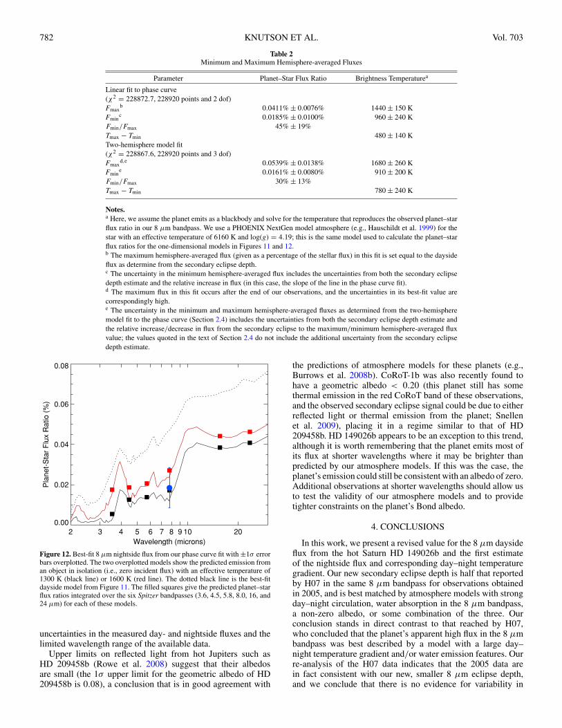
782 KNUTSON ET AL. Vol. 703
Table 2Minimum and Maximum Hemisphere-averaged Fluxes
Parameter Planet–Star Flux Ratio Brightness Temperaturea
Linear fit to phase curve(χ2 = 228872.7, 228920 points and 2 dof)Fmax
b 0.0411% ± 0.0076% 1440 ± 150 KFmin
c 0.0185% ± 0.0100% 960 ± 240 KFmin/Fmax 45% ± 19%Tmax − Tmin 480 ± 140 KTwo-hemisphere model fit(χ2 = 228867.6, 228920 points and 3 dof)Fmax
d,e 0.0539% ± 0.0138% 1680 ± 260 KFmin
e 0.0161% ± 0.0080% 910 ± 200 KFmin/Fmax 30% ± 13%Tmax − Tmin 780 ± 240 K
Notes.a Here, we assume the planet emits as a blackbody and solve for the temperature that reproduces the observed planet–starflux ratio in our 8 μm bandpass. We use a PHOENIX NextGen model atmosphere (e.g., Hauschildt et al. 1999) for thestar with an effective temperature of 6160 K and log(g) = 4.19; this is the same model used to calculate the planet–starflux ratios for the one-dimensional models in Figures 11 and 12.b The maximum hemisphere-averaged flux (given as a percentage of the stellar flux) in this fit is set equal to the daysideflux as determine from the secondary eclipse depth.c The uncertainty in the minimum hemisphere-averaged flux includes the uncertainties from both the secondary eclipsedepth estimate and the relative increase in flux (in this case, the slope of the line in the phase curve fit).d The maximum flux in this fit occurs after the end of our observations, and the uncertainties in its best-fit value arecorrespondingly high.e The uncertainty in the minimum and maximum hemisphere-averaged fluxes as determined from the two-hemispheremodel fit to the phase curve (Section 2.4) includes the uncertainties from both the secondary eclipse depth estimate andthe relative increase/decrease in flux from the secondary eclipse to the maximum/minimum hemisphere-averaged fluxvalue; the values quoted in the text of Section 2.4 do not include the additional uncertainty from the secondary eclipsedepth estimate.
2 3 4 5 6 7 8 9 10 20Wavelength (microns)
0.00
0.02
0.04
0.06
0.08
Pla
net-
Sta
r F
lux
Ratio
(%
)
Figure 12. Best-fit 8 μm nightside flux from our phase curve fit with ±1σ errorbars overplotted. The two overplotted models show the predicted emission froman object in isolation (i.e., zero incident flux) with an effective temperature of1300 K (black line) or 1600 K (red line). The dotted black line is the best-fitdayside model from Figure 11. The filled squares give the predicted planet–starflux ratios integrated over the six Spitzer bandpasses (3.6, 4.5, 5.8, 8.0, 16, and24 μm) for each of these models.
uncertainties in the measured day- and nightside fluxes and thelimited wavelength range of the available data.
Upper limits on reflected light from hot Jupiters such asHD 209458b (Rowe et al. 2008) suggest that their albedosare small (the 1σ upper limit for the geometric albedo of HD209458b is 0.08), a conclusion that is in good agreement with
the predictions of atmosphere models for these planets (e.g.,Burrows et al. 2008b). CoRoT-1b was also recently found tohave a geometric albedo < 0.20 (this planet still has somethermal emission in the red CoRoT band of these observations,and the observed secondary eclipse signal could be due to eitherreflected light or thermal emission from the planet; Snellenet al. 2009), placing it in a regime similar to that of HD209458b. HD 149026b appears to be an exception to this trend,although it is worth remembering that the planet emits most ofits flux at shorter wavelengths where it may be brighter thanpredicted by our atmosphere models. If this was the case, theplanet’s emission could still be consistent with an albedo of zero.Additional observations at shorter wavelengths should allow usto test the validity of our atmosphere models and to providetighter constraints on the planet’s Bond albedo.
4. CONCLUSIONS
In this work, we present a revised value for the 8 μm daysideflux from the hot Saturn HD 149026b and the first estimateof the nightside flux and corresponding day–night temperaturegradient. Our new secondary eclipse depth is half that reportedby H07 in the same 8 μm bandpass for observations obtainedin 2005, and is best matched by atmosphere models with strongday–night circulation, water absorption in the 8 μm bandpass,a non-zero albedo, or some combination of the three. Ourconclusion stands in direct contrast to that reached by H07,who concluded that the planet’s apparent high flux in the 8 μmbandpass was best described by a model with a large day–night temperature gradient and/or water emission features. Ourre-analysis of the H07 data indicates that the 2005 data arein fact consistent with our new, smaller 8 μm eclipse depth,and we conclude that there is no evidence for variability in
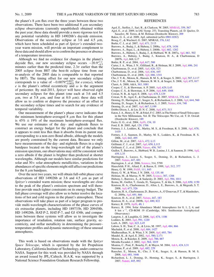
No. 1, 2009 THE 8 μm PHASE VARIATION OF THE HOT SATURN HD 149026b 783
the planet’s 8 μm flux over the three years between these twoobservations. There have been two additional 8 μm secondaryeclipse observations (currently unpublished) obtained withinthe past year; these data should provide a more rigorous test forany potential variability in HD 149026b’s dayside emission.Observations of the secondary eclipse at 3.6 and 4.5 μm,which have been scheduled as part of Spitzer’s extended two-year warm mission, will provide an important complement tothese data and should allow us to confirm the presence or absenceof a temperature inversion.
Although we find no evidence for changes in the planet’sdayside flux, our new secondary eclipse occurs −20.9+7.2
−6.5minutes earlier than the predicted time, 2.3σ earlier than the2005 eclipse from H07 (the best-fit eclipse time from ourre-analysis of the 2005 data is comparable to that reportedby H07). The timing offset for our new secondary eclipsecorresponds to a value of −0.0079+0.0027
−0.0025 for e cos(ω), wheree is the planet’s orbital eccentricity and ω is the argumentof pericenter. By mid-2011, Spitzer will have observed eightsecondary eclipses for this planet (one each at 3.6 and 4.5μm, two at 5.8 μm, and four at 8.0 μm); these data willallow us to confirm or disprove the presence of an offset inthe secondary eclipse times and to search for any evidence oftemporal variability.
Our measurement of the planet’s phase curve indicates thatthe minimum hemisphere-averaged 8 μm flux for this planetis 45% ± 19% of the maximum hemisphere-averaged flux.We use our estimates of the day- and nightside fluxes toconstruct an energy budget for the planet and conclude thatit appears to emit less flux than it absorbs from its parent star,corresponding to a non-zero Bond albedo, although the modelsare poorly constrained by the current data. Because we onlyhave measurements of the day- and nightside fluxes in a singlebandpass located on the long-wavelength tail of the planet’semission spectrum, our observations may still be consistent witha zero albedo if the planet is brighter than predicted at shorterwavelengths. Although our models have similar predictions forsolar and 30× solar atmospheric metallicities, variations in theabundances of specific elements might still affect our predictionsfor the 8 μm bandpass.
Over the next two years, we will obtain full-orbit phase curveobservations of HD 149026b at 3.6 and 4.5 μm as part ofSpitzer’s extended warm mission; these wavelengths are closeto the peak of the planet’s emission spectrum and will there-fore provide much tighter constraints on its energy budget. Thefull phase coverage will also allow us to better resolve the loca-tions of hot and cold regions in the planet’s atmosphere. Theseobservations will take place as part of a larger program to pro-vide multi-wavelength characterizations of the phase curves ofsix extrasolar planets, including HD 189733b, HD 209458b,HD 149026b, HAT-P-2, HAT-P-7, and GJ 436b, and compar-isons between these systems will allow us to investigate theimportance of irradiation, rotation rate, surface gravity, ec-centricity, and stellar metallicity in determining the pressure–temperature profiles and dynamic meteorology of these unusualatmospheres.
This work is based on observations made with the SpitzerSpace Telescope, which is operated by the Jet PropulsionLaboratory, California Institute of Technology, under contract toNASA. Support for this work was provided by NASA throughan award issued by JPL/Caltech. H.A.K. was supported by aNational Science Foundation Graduate Research Fellowship.
REFERENCES
Agol, E., Steffen, J., Sari, R., & Clarkson, W. 2005, MNRAS, 359, 567Agol, E., et al. 2009, in IAU Symp. 253, Transiting Planets, ed. D. Queloz, D.
Sasselov, M. Torres, & M. Holman (Dordrecht: Kluwer), 209Bakos, G. A., et al. 2009, ApJ, submitted (arXiv:0901.0282)Broeg, C., & Wuchterl, G. 2007, MNRAS, 376, L62Burke, C. J., et al. 2007, ApJ, 671, 2115Burrows, A., Budaj, J., & Hubeny, I. 2008a, ApJ, 678, 1436Burrows, A., Ibgui, L., & Hubeny, I. 2008b, ApJ, 682, 1282Burrows, A., Hubeny, I., Budaj, J., & Hubbard, W. B. 2007a, ApJ, 661, 502Burrows, A., Hubeny, I., Budaj, J., Knutson, H. A., & Charbonneau, D
2007b, ApJ, 668, L17Butler, R. P., et al. 2004, ApJ, 617, 580Carter, J. A., Winn, J. N., Gilliland, R., & Holman, M. J. 2009, ApJ, 696, 241Charbonneau, D., et al. 2005, ApJ, 626, 523Charbonneau, D., et al. 2006, ApJ, 636, 445Charbonneau, D., et al. 2008, ApJ, 686, 1341Cho, J. Y.-K., Menou, K., Hansen, B. M. S., & Seager, S. 2003, ApJ, 587, L117Cho, J. Y.-K., Menou, K., Hansen, B. M. S., & Seager, S. 2008, ApJ, 675, 817Claret, A. 2000, A&A, 363, 1081Cooper, C. S., & Showman, A. P. 2005, ApJ, 629, L45Cooper, C. S., & Showman, A. P. 2006, ApJ, 649, 1048Cowan, N. B., & Agol, E. 2008, ApJ, 678, L129Cowan, N. B., Agol, E., & Charbonneau, D. 2007, MNRAS, 379, 641Deming, D., Harrington, J., Seager, S., & Richardson, L. J. 2006, ApJ, 644, 560Deming, D., Seager, S., & Richardson, L. J. 2005, Nature, 434, 740Deming, D., et al. 2007, ApJ, 667, L199Dobbs-Dixon, I., & Lin, D. N. C. 2008, ApJ, 673, 513Eaton, J. A., Henry, G. W., & Fekel, F. C. 2003, in The Future of Small Telescopes
in the New Millennium, Vol. II: The Telescopes We Use, ed. T. D. Oswalt(Dordrecht: Kluwer), 189
Fazio, G. G., et al. 2004, ApJS, 154, 10Ford, E. B. 2005, ApJ, 129, 1706Fortney, J. J., Lodders, K., Marley, M. S., & Freedman, R. S. 2008, ApJ, 678,
1419Fortney, J. J., Saumon, D., Marley, M. S., Lodders, K., & Freedman, R. S.
2006, ApJ, 642, 495Gillon, M., et al. 2007, A&A, 472, L13Grillmair, C. J., et al. 2007, ApJ, 658, L115Grillmair, C. J., et al. 2009, Nature, 456, 767Guillot, T., Burrows, A., Hubbard, W. B., Lunine, J. I., & Saumon, D. 1996, ApJ,
459, L35Harrington, J., Luszcz, S., Seager, S., Deming, D., & Richardson, L. J.
2007, Nature, 447, 691Harrington, J., et al. 2006, Science, 314, 5799Hauschildt, P. H., Allard, F., & Baron, E. 1999, ApJ, 512, 377Henry, G. W. 1999, PASP, 111, 845Henry, G. W., & Winn, J. N. 2008, AJ, 135, 68Holman, M., & Murray, N. W. 2005, Science, 307, 1288Hubeny, I., Burrows, A., & Sudarsky, D. 2003, ApJ, 594, 1011Ikoma, M., Guillot, T., Genda, H., Tanigawa, T., & Ida, S. 2006, ApJ, 650, 1150Knutson, H. A., Charbonneau, D., Allen, L. E., Burrows, A., & Megeath, S. T.
2008, ApJ, 673, 526Knutson, H. A., Charbonneau, D., Burrows, A., O’Donovan, F. T., & Mandushev,
G. 2009a, ApJ, 691, 866Knutson, H. A., et al. 2007, Nature, 447, 183Knutson, H. A., et al. 2009b, ApJ, 690, 822Kurucz, R. 1979, ApJS, 40, 1Kurucz, R. 1994, Solar Abundance Model Atmospheres for 0, 1, 2, 4, and
8 km s−1, CD-ROM 19 (Cambridge, MA: Smithsonian AstrophysicalObservatory)
Langton, J., & Laughlin, G. 2008, ApJ, 674, 1106Lodders, K. 2003, ApJ, 591, 1220Loeb, A. 2005, ApJ, 623, L45Lubow, S. H., Tout, C. A., & Livio, M. 1997, ApJ, 484, 866Machalek, P., et al. 2008, ApJ, 684, 1427Madhusudhan, N., & Winn, J. N. 2009, ApJ, 693, 784Mandel, K., & Agol, E. 2002, ApJ, 580, L171Menou, K., & Rausher, E. 2009, ApJ, 700, 887Miralda Escudee, J. 2002, ApJ, 564, 1019Moutou, C., Pont, F., Bouchy, F., & Mayor, M. 2004, A&A, 424, L31Nutzman, P., et al. 2009, ApJ, 692, 229Rauscher, E., Menou, K., Cho, J. Y.-K., Seager, S., & Hansen, B. M. S.
2008, ApJ, 681, 1646Richardson, L. J., Deming, D., Horning, K., Seager, S., & Harrington, J.
2007, Nature, 445, 892
784 KNUTSON ET AL. Vol. 703
Rowe, J. F., et al. 2008, ApJ, 689, 1345Sato, B., et al. 2005, ApJ, 633, 465Snellen, I. A. G., de Mooij, E. J. W., & Albrecht, S. 2009, Nature, 459, 543Showman, A. P., & Guillot, T. 2002, A&A, 385, 166Showman, A. P., et al. 2008, ApJ, 682, 559Showman, A. P., et al. 2009, ApJ, 699, 564Spiegel, D. S., Silverio, K., & Burrows, A. 2009, ApJ, 699, 1487Tegmark, M., et al. 2004, Phys. Rev. D, 69, 103501
Werner, M. W., et al. 2004, ApJS, 154, 1Winn, J. N., Holman, M. J., & Roussanova, A. 2007a, ApJ, 657,
1098Winn, J. N., et al. 2007b, AJ, 133, 1828Winn, J. N., et al. 2008, ApJ, 675, 1531Wolf, A. S., et al. 2007, ApJ, 667, 549Zahnle, K., Marley, M. S., Freedman, R. S., Lodders, K., & Fortney, J. J.
2009, ApJ, 701, L20


![TUSSO | Espresso v4 [HD] - EL](https://static.fdocument.org/doc/165x107/544fd122af7959e1108b9656/tusso-espresso-v4-hd-el.jpg)