Reliability Analysis of Logic Circuitskmram/publications/tcad09.pdfDigital Object Identiﬁer...

392 IEEE TRANSACTIONS ON COMPUTER-AIDED DESIGN OF INTEGRATED CIRCUITS AND SYSTEMS, VOL. 28, NO. 3, MARCH 2009

Reliability Analysis of Logic CircuitsMihir R. Choudhury, Student Member, IEEE, and Kartik Mohanram, Member, IEEE

Abstract—Reliability of logic circuits is emerging as an impor-tant concern in scaled electronic technologies. Reliability analysisof logic circuits is computationally complex because of the expo-nential number of inputs, combinations, and correlations in gatefailures. This paper presents three accurate and scalable algo-rithms for reliability analysis of logic circuits. The first algorithm,called observability-based reliability analysis, provides a closed-form expression for reliability and is accurate when single gatefailures are dominant in a logic circuit. The second algorithm,called single-pass reliability analysis, computes reliability in asingle topological walk through the logic circuit. It computes theexact reliability for circuits without reconvergent fan-out, evenin the presence of multiple gate failures. The algorithm can alsohandle circuits with reconvergent fan-out with high accuracy usingcorrelation coefficients as described in this paper. The third algo-rithm, called maximum-k gate failure reliability analysis, allowsa constraint on the maximum number (k) of gates that can failsimultaneously in a logic circuit. Simulation results for severalbenchmark circuits demonstrate the accuracy, performance, andpotential applications of the proposed algorithms.

Index Terms—Gate failures, logic circuits, reliability analysis.

I. INTRODUCTION

I T IS WIDELY acknowledged that there will be a sharpincrease in manufacturing defect levels and transient fault

rates in future electronic technologies, e.g., [1]–[5]. Defectsand faults impact performance and limit the reliability of elec-tronic systems. This has led to considerable interest in practicaltechniques for reliability analysis that are accurate, robust, andscalable with design complexity. Reliability analysis of logiccircuits refers to the problem of evaluating the effects of errorsdue to noise at individual transistors, gates, or logic blocks onthe outputs of the circuit. The models for noise range fromhighly specific decomposition of the sources, e.g., single-eventupsets, to highly abstract models that combine the effects ofdifferent failure mechanisms.

Reliability analysis of logic circuits is computationally com-plex because of the exponential number of inputs, combina-tions, and correlations in gate failures. Standard techniquesfor reliability analysis use fault injection and simulation ina Monte Carlo framework. Although parallelizable, they arestill not efficient for use on large circuits. Analytical methods

Manuscript received April 10, 2008; revised July 23, 2008. Current versionpublished February 19, 2009. This research was supported in part by CAREERAward CCF-0746850 from the National Science Foundation and in part by theA. Richard Newton Graduate Scholarship. This paper was recommended byAssociate Editor N. K. Jha.

The authors are with the Department of Electrical and Computer Engi-neering, Rice University, Houston, TX 77005 USA (e-mail: [email protected];[email protected]).

Color versions of one or more of the figures in this paper are available onlineat http://ieeexplore.ieee.org.

Digital Object Identifier 10.1109/TCAD.2009.2012530

for reliability analysis are applicable to very simple structuressuch as two-input and three-input gates, and regular fabrics [6],[7]. Although they can be applied to large multilevel circuitswith simplifying assumptions and compositional rules, there isa significant loss in accuracy. Recent advances in reliabilityanalysis are based on probabilistic transfer matrices (PTMs)[8], Bayesian networks [9], and Markov random fields [10],[11]. However, all approaches require significant runtimes forsmall benchmark circuits. In the PTM approach, this can beattributed to the storage and manipulation of large algebraicdecision diagrams (ADDs) used to represent the probabilisticbehavior of the circuit. In the Bayesian network approach, thelarge runtimes arise from large conditional probability tablesthat support Bayesian network operations. The use of Markovrandom fields becomes computationally intensive for arbitrarymultilevel logic circuits because it involves minimization of acomplex Gibbs distribution function with a large number ofvariables. Many reliability analysis techniques have been pro-posed in the context of soft errors [12], [13]. These techniquespredict soft error rate in circuits, accounting for electricalmasking, and latching-window masking in addition to logicalmasking. Since these techniques are specific to soft errors, theyfocus mainly on predicting single gate failure effects.

This paper presents three accurate and scalable algorithmsfor reliability analysis of logic circuits. The first algorithm,called observability-based reliability analysis, uses observabil-ity metrics to quantify the impact of a gate failure on the outputof the circuit. The observability-based approach provides aclosed-form expression for circuit reliability as a function ofthe failure probabilities and observabilities of the gates. Theclosed-form expression is accurate when the probability of asingle gate failure is significantly higher than the probability ofmultiple gate failures.

The second algorithm, called single-pass reliability analysis,leverages insights into the effects of multiple gate failuresderived from observability-based reliability analysis. In this al-gorithm, gates are topologically sorted and processed in a singlepass from the inputs to the outputs. Topological sorting ensuresthat before a gate is processed, the effects of multiple gate fail-ures in the transitive fan-in cone of the gate are computed andstored at the inputs of the gate. Using the joint signal prob-ability distribution of the gate’s inputs, the propagated errorprobabilities from its transitive fan-in stored at its inputs, andthe failure probability of the gate, the cumulative effect offailures are computed at the output of the gate. The single-pass reliability analysis algorithm is provably exact for circuitswithout reconvergent fan-out. Reconvergent fan-out introducescorrelations when error probabilities are combined at the pointof reconvergence, which is handled using correlation coeffi-cients. The accuracy of the algorithm can be improved by using

0278-0070/$25.00 © 2009 IEEE

Authorized licensed use limited to: Rice University. Downloaded on April 14, 2009 at 14:05 from IEEE Xplore. Restrictions apply.

CHOUDHURY AND MOHANRAM: RELIABILITY ANALYSIS OF LOGIC CIRCUITS 393

higher order correlation coefficients to capture the correlationeffects. However, the computational complexity increases asthe number of correlation coefficients increases. This paperexplores the tradeoff between accuracy and computational com-plexity for 0, 4, and 16 correlation coefficients.

The above algorithms for reliability analysis use an indepen-dent gate failure model, in which there is a nonzero probabilityof a large number of gates failing simultaneously. However, inpractice, it is reasonable to expect an upper bound, k, on themaximum number of gates that can fail simultaneously in thelogic circuit. Termed the maximum-k gate failure model,the gate failures remain independent although the global con-straint due to the upper bound k introduces correlation amonggate failures. The third algorithm, called maximum-k gate fail-ure reliability analysis, is based on a technique that generatesa set of gate failures (of cardinality ≤ k) according to theindependent gate failure model. Given this set of gate failures,single-pass reliability analysis is used to evaluate their effecton the output(s) of the circuit. For a logic circuit with N gates,generating samples of failed gates is challenging because thesize of the sample space is O(Nk) and all brute-force solutionsare computationally intensive. The sampling algorithm pro-posed in this paper has a computational complexity of O(Nk2).Simulation results for several benchmark circuits demonstratethe accuracy, performance, and potential applications of theproposed analysis algorithms to guide logic design for bothredundancy-free and redundancy-based reliability enhancementin logic circuits [14]–[16].

This paper is an extended version of [17] and is organized asfollows. Section II provides a background in reliability analysis.Section III describes the observability-based algorithm for reli-ability analysis. Section IV describes the single-pass algorithmfor reliability analysis. Section V describes the maximum-kgate failure model and an efficient algorithm for reliabilityanalysis. Section VI presents simulation results. Section VII isa conclusion.

II. BACKGROUND

The classical model for errors due to noise in a logic circuitwas introduced by von Neumann in 1956 [6]. Noise at a gate ismodeled as a binary symmetric channel (BSC), with a crossoverprobability ε. In other words, following the computation at thegate, the BSC can cause the gate output to toggle symmetrically(from 0 → 1 or 1 → 0) with the same probability of error, ε.Each gate has an ε ∈ [0, 0.5] associated with it, where ε equalszero for an error-free gate, and ε equals 0.5 for a perfectlynoisy gate (a gate with random output). It is unrealistic for agate to have ε > 0.5 because it would mean that the outputof the gate is more likely to be faulty than correct. In such acase, adding a NOT gate at the output of the gate would makethe combination of the two gates more reliable. For example,if an AND gate in a circuit has a failure probability 0.7, thenadding a NOT gate with a failure probability x at the output ofthe AND gate means that the failure probability of the combi-nation is ε′ = 0.7x + 0.3(1 − x). For any value of x in [0,1],ε′ ≤ 0.7. Hence, in this paper, we only consider gate failureprobability in [0, 0.5]. Note that gates are assumed to fail in-

dependently of each other. Although this may not be a realisticassumption, since effects of noise are potentially localized andcorrelated, it helps to simplify reliability analysis while stillproviding valuable insights into circuit reliability. In this paper,the phrases “gate is in error,” “erroneous gate,” and “gate hasfailed” are used to mean that a particular gate is known toproduce an incorrect output.

The BSC model allows the effects of different sources ofnoise such as crosstalk, terrestrial cosmic radiation, electro-magnetic interference, etc., to be combined into the failureprobability ε. At the electrical level, the effects of noise canusually be modeled by a probability distribution about thenominal voltage, instead of a single number. Traditionally, aGaussian distribution has been shown to be a good approxima-tion for this distribution. Reliability analysis is a problem in thediscrete domain (involving Boolean logic) and the noise at thegates, modeled by a Gaussian distribution, is in the continuousdomain. As a result, reliability analysis would require Booleanoperations on Gaussian distributions to propagate errors fromgate inputs to the output. Since the resulting distribution maynot be Gaussian, either scalability or accuracy will be lost in thisapproach. Since there are multiple sources of noise and since itis desirable to work with a higher abstraction for the combinedeffects of these sources, the Gaussian model for noise is dis-cretized by computing the probability that the nominal voltageexceeds the noise margin for both low and high output voltages.Without loss of generality, the average probability that the lowand high voltages exceed the noise margin is used to estimatethe gate failure probability ε for the rest of this paper. Note thatall the algorithms proposed in this paper can be extended tohandle 0 → 1 and 1 → 0 gate failure probabilities separately.

Reliability of a logic circuit is defined as the probability oferror at the output of the logic circuit δ as a function of failureprobabilities �ε of the gates, where �ε is the vector containingthe failure probabilities {ε1, ε2, . . .} of the gates in the circuit.Reliability δ(�ε) can lie in the interval from zero to one. Theexpected number of simultaneous gate failures is given by∑

εi. Thus, the value of εis determines the distribution of thenumber of simultaneous gate failures. Note that if εi �= 0∀i,then the number of simultaneous gate failures can vary fromzero to all the gates in the circuit with some nonzero probability(although the probability of a large number of simultaneousgate failures is very low). Such a wide range for the numberof gate failures is an artifact of the independent gate failuremodel. The independent gate failure model can be improved byimposing a limit on the number of simultaneous gate failures.For instance, in the single gate failure model, the limit is one.This paper describes an efficient reliability analysis algorithmwhen the limit on the number of simultaneous gate failures isk ≤ N .

In special cases, reliability analysis can leverage existingtechniques from switching activity computation [18] and ob-servability computation [19]. If failures at only the primaryinputs of the circuit are considered, and gates are assumed tobe error free, then the problem of reliability analysis can besolved using switching activity computation algorithms. The0 → 1 and 1 → 0 error probabilities can be thought of as theswitching probability, and the switching activity of every gate



can be computed. The resulting 0 → 1 and 1 → 0 switchingprobabilities at a gate are the error probabilities at that gate.However, in the general case, reliability analysis becomes morecomplex when gate failures are also considered, because ofthe exponential number of combinations of gate failures. Ifonly single gate failures are considered, the reliability analysisproblem can be solved by simply computing the observabilityof the gates. The contribution of each gate to the error proba-bility of an output (y) is given by the failure probability of thegate (ε) times the observability of the gate at the output y. Inthe general case, reliability analysis for multiple gate failuresbecomes more complex because the observabilities of the gatesare not independent of each other, and the gate failures canchange observability of the gates. These effects are describedin greater detail in Section III-A.

The traditional approach to reliability analysis uses faultinjection and simulation in a Monte Carlo framework. Recentprogress in reliability analysis has seen the use of PTMs [8],Bayesian networks [9], and Markov random fields [10], [11].Without exception, these approaches suffer from the problemof scalability. Monte Carlo simulations have the added dis-advantage of inflexibility, since the entire simulation has tobe repeated for any change in circuit structure or �ε. PTM-based reliability analysis uses transfer matrices to representinput–output behavior of noisy circuits. PTMs store the prob-ability of occurrence of every input–output vector pair for eachlevel in the circuit to compute the probability of error at theoutput of the circuit. This leads to massive matrix storage andmanipulation overhead. Even with compaction of the matri-ces using ADDs, the high runtimes reported for benchmarkcircuits with 20–50 gates suggest their inapplicability to largecircuits. Although this problem is somewhat mitigated in theBayesian network approach for small circuits, manipulatingBayesian networks for large circuits is potentially intractable.A probabilistic design methodology based on Markov randomfields is presented in [10] that uses the Gibbs distribution tocharacterize reliability in terms of entropy and noise in terms ofthermal energy. Evaluating reliability using this technique be-comes computationally intensive for arbitrary multilevel logiccircuits because it involves minimization of a complex Gibbsdistribution function with a large number of variables. Thistechnique is more suitable for evaluating reliability of regularredundancy architectures like triple modular redundancy andNAND multiplexing [11]. Alternatively, analytical approachesdeveloped to study fault-tolerant approaches like NAND multi-plexing and majority voting can be used for reliability analysis[6], [7]. However, the simple compositional rules that theseapproaches use work best on regular structures. When used onirregular multilevel structures such as logic circuits, they suffersignificant penalties in accuracy even on small circuits.

III. OBSERVABILITY-BASED RELIABILITY ANALYSIS

In this section, an intuitive approach to reliability analysis isdescribed. It is based upon the observation that a failure at agate close to the primary output has a greater probability ofpropagating to the primary output than a gate several levelsof logic away from the primary outputs. This is because a

failure that has to propagate through several levels of logic hasa higher probability of being logically masked. This can bequantified by applying the concept of observability [19], whichhas historically found use in the testing and logic synthesisdomains [20].

For reliability analysis, the observability of any wire in thecircuit can be defined as the probability that a 0 → 1 or 1 → 0error at that wire affects the output of the circuit. Note thatthe observabilities are the noiseless observabilities, i.e., all thegates are assumed noise-free when the observabilities are cal-culated. Observabilities can be calculated using Boolean differ-ences, symbolic techniques based on binary decision diagrams(BDDs), or simulation. Using the observabilities, a closed-formexpression for the reliability, δy(�ε), is derived.

Let us begin with the trivial case of a circuit with a singlegate having a failure probability ε. Since there is only one gate,the output of the gate is the primary output of the circuit and hasan observability o of 1. Hence, the probability of failure of theoutput is equal to ε · o = ε. Now, consider the case of a circuitwith two cascaded gates g1 and g2 having failure probabilitiesε1 and ε2 and observabilities o1 and o2. When both gates areerror free, the primary output of the circuit is always error free.When at least one gate is in error, the error at the primary outputis computed by analyzing two cases when 1) only one gate is inerror and 2) both g1 and g2 are in error. When exactly one gatehas failed, the primary output is in error when the failed gateis observable. Hence, the first error component of the output isε1(1 − ε2)o1 + (1 − ε1)ε2o2.

When both g1 and g2 are in error, the primary output is inerror when g1 and g2 are jointly observable. Joint observabilityof two gates g1 and g2 is the probability that the primaryoutput toggles when the outputs of both g1 and g2 toggle. Notethat the joint observability is different from the simultaneousobservability of g1 and g2, which is the probability that atoggle at g1 causes a toggle at the primary output and a toggleat g2 also causes a toggle at the primary output. Computingjoint observability for all combinations of multiple gate failuresis expensive because joint observability computation is itselfcomputationally demanding and the number of combinationsof multiple gate failures is exponential in the number of gatesin the circuit. Thus, observability-based reliability analysismakes two simplifying assumptions for estimating the effect ofmultiple gate failures.

1) The effect of gate failures at the primary output aredecoupled from each other, i.e., a failure at each gate gi

is assumed to affect the output with a probability oi

regardless of other gate failures. This assumption allowsthe joint observability to be replaced by simultaneous ob-servability, which is computationally less demanding, tocompute the effect of multiple gate failures at the output.

2) The observability of the gates are assumed to be inde-pendent of each other. Using this assumption, the compu-tation of simultaneous observability of two gates can besimplified to the product of the individual gate observabil-ities. For instance, the probability that g1 is observableand g2 is not observable is given by o1(1 − o2) and theprobability that g1 and g2 are both not observable is givenby (1 − o1)(1 − o2).



Let Ω be the set of all the gates in the circuit and S be theset of all nonempty subsets of Ω. Consider a set G ∈ S ofgates that have failed. The exact effect of these failed gates isgiven by the joint observability of the gates in G. Using the firstassumption, it can be argued that the output is in error wheneveran odd number of gates in G are simultaneously observable.Using the same assumption, when an even number of gatesin G are simultaneously observable, the effect of these gatefailures cancel each other. Thus, the joint observability of gatesin G is estimated as the sum of simultaneous observability ofan odd number of gates in G. Using the second assumption,the simultaneous observability of the two gates is given bythe product of their individual observabilities. Note that inpractice, there are cases when an odd number of simultaneouslyobservable gates in G do not cause an error at the primaryoutput and also cases when an even number of simultaneouslyobservable gates in G cause an error at the primary output.These are averaged and absorbed into the probability of an oddnumber of failed gates being simultaneously observable by thefirst assumption.

For the two gate example described above, the second errorcomponent of the output (both gates in error) is given byε1ε2(o1(1 − o2) + o2(1 − o1)). The first term o1(1 − o2) isthe probability that g1 is observable and g2 is not and viceversa for the second term. The joint observability of g1 andg2 is estimated by o1(1 − o2) + o2(1 − o1) (odd number oferroneous gates being simultaneously observable). The inaccu-racies introduced due to the two simplifying assumptions areillustrated with an example in Section III-A.

With this background, we shall derive the expression forthe probability of error at the output for a general circuitwith N gates. Without loss of generality, we assume that thecircuit has a single output y. Denote the error probability(observability) of the ith gate by εi(oi). Let 2G denotes theset of all subsets of G. Let F ∈ 2G be the set of gates in Gthat are simultaneously observable. Using the first assumption,the output y will be in error when an odd number of gatesin G are simultaneously observable, i.e., F contains an oddnumber of gates. Using the second assumption, the simul-taneous observability of a set of gates can be computed bysimply multiplying the individual observabilities of the gates.For instance, if G contains three gates (g1, g2, and g3) andF = {g1, g2}, then the probability that g1 and g2 are simulta-neously observable is given by o1o2(1 − o3). In general, theprobability that the gates in F are observable is given by A =∏

i/∈F (1 − oi)∏

j∈F oj . The expression B =∏

i/∈F (1 − oi)∏j∈F −oj has the same magnitude as A and same sign as A

when F has an even number of gates, and opposite sign asA when F has an odd number of gates. Thus, when F hasan odd number of gates, the expression 1/2(A − B) gives theprobability that the gates in F are observable, and when F hasan even number of gates 1/2(A − B) is equal to zero. Thus, theprobability that an odd number of gates in G are observable isgiven by

∑F∈2G

12

⎛⎝∏

i/∈F

(1 − oi)∏j∈F

oj −∏i/∈F

(1 − oi)∏j∈F

−oj

⎞⎠ . (1)

By the first simplifying assumption, the probability of error atthe output y(yerror) given that the gates in G have failed is alsogiven by (1). Thus

Pr(yerror|G) =12

⎛⎝∑

F∈2G

∏i/∈F

(1 − oi)∏j∈F

oj

−∑

F∈2G

∏i/∈F

(1 − oi)∏j∈F

−oj

⎞⎠

= 1/2

⎛⎝∏

j∈G

(oj +(1−oj))−∏j∈G

((1−oj)−oj)

⎞⎠

= 1/2

⎛⎝1 −

∏j∈G

(1 − 2oj)

⎞⎠ .

The probability that the gates in G are in error and the gates inGc(Ω \ G) are error free is given by

∏i∈G εi

∏j∈Gc(1 − εj).

Thus, the probability of error at the output y is given by

Pr(yerror) =∑G∈S

∏i∈G

εi

∏j∈Gc

(1 − εj)

×(1 −∏j∈G(1 − 2oj)

2

)⇒ Pr(yerror) = 1/2

∑G∈S

∏i∈G

εi

∏j∈Gc

(1 − εj)

− 1/2∑G∈S

∏i∈G

εi(1 − 2oi)∏

j∈Gc

(1 − εj).

Since S contains all nonempty subsets of Ω, the firstterm

∑G∈S

∏i∈G εi

∏j∈Gc(1 − εj) contains all the terms in∏

i∈Ω((1 − εi) + εi) (when it is expanded) except∏

i∈Ω(1 −εi). Hence, the first term can be replaced by∏

i∈Ω

(1 − εi + εi) −∏i∈Ω

(1 − εi) = 1 −∏i∈Ω

(1 − εi).

A similar transformation for the second term yields

Pr(yerror)=1/2

(1−∏i∈Ω

(1−εi)

)

−1/2

(∏i∈Ω

(1−εi+εi(1−2oi))−∏i∈Ω

(1−εi)

)

⇒ Pr(yerror)=1/2

(1−∏i∈Ω

(1−2εioi)

). (2)

Equation (2) is a closed-form expression for the reliabilityof the output of a circuit as a function of error probabilitiesat each gate. Since the product of (1 − 2εioi) is over all gatesin the circuit, it can be computed very efficiently once theobservability of each gate is known. It is interesting to notethat the closed-form expression computes the exact expressionfor reliability of an XOR tree circuit. The observabilities of theXOR gates in the tree are independent and always equal to oneirrespective of other XOR gate failures in the tree. Thus, the twosimplifying assumptions of the observability-based reliability



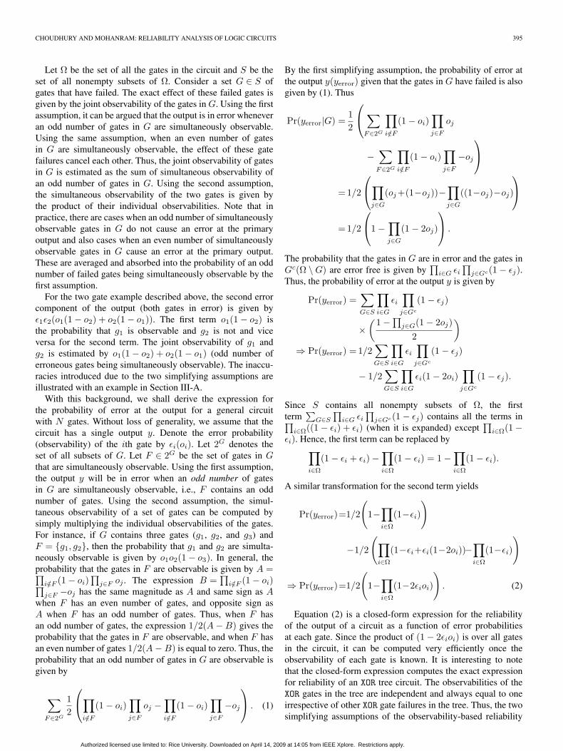
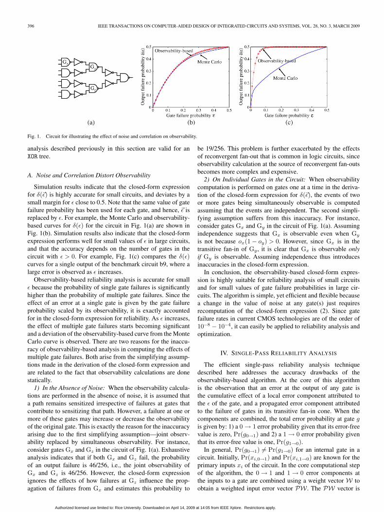
Fig. 1. Circuit for illustrating the effect of noise and correlation on observability.

analysis described previously in this section are valid for anXOR tree.

A. Noise and Correlation Distort Observability

Simulation results indicate that the closed-form expressionfor δ(�ε) is highly accurate for small circuits, and deviates by asmall margin for ε close to 0.5. Note that the same value of gatefailure probability has been used for each gate, and hence, �ε isreplaced by ε. For example, the Monte Carlo and observability-based curves for δ(ε) for the circuit in Fig. 1(a) are shown inFig. 1(b). Simulation results also indicate that the closed-formexpression performs well for small values of ε in large circuits,and that the accuracy depends on the number of gates in thecircuit with ε > 0. For example, Fig. 1(c) compares the δ(ε)curves for a single output of the benchmark circuit b9, where alarge error is observed as ε increases.

Observability-based reliability analysis is accurate for smallε because the probability of single gate failures is significantlyhigher than the probability of multiple gate failures. Since theeffect of an error at a single gate is given by the gate failureprobability scaled by its observability, it is exactly accountedfor in the closed-form expression for reliability. As ε increases,the effect of multiple gate failures starts becoming significantand a deviation of the observability-based curve from the MonteCarlo curve is observed. There are two reasons for the inaccu-racy of observability-based analysis in computing the effects ofmultiple gate failures. Both arise from the simplifying assump-tions made in the derivation of the closed-form expression andare related to the fact that observability calculations are donestatically.

1) In the Absence of Noise: When the observability calcula-tions are performed in the absence of noise, it is assumed thata path remains sensitized irrespective of failures at gates thatcontribute to sensitizing that path. However, a failure at one ormore of these gates may increase or decrease the observabilityof the original gate. This is exactly the reason for the inaccuracyarising due to the first simplifying assumption—joint observ-ability replaced by simultaneous observability. For instance,consider gates Gx and Gz in the circuit of Fig. 1(a). Exhaustiveanalysis indicates that if both Gx and Gz fail, the probabilityof an output failure is 46/256, i.e., the joint observability ofGx and Gz is 46/256. However, the closed-form expressionignores the effects of how failures at Gz influence the prop-agation of failures from Gx and estimates this probability to

be 19/256. This problem is further exacerbated by the effectsof reconvergent fan-out that is common in logic circuits, sinceobservability calculation at the source of reconvergent fan-outsbecomes more complex and expensive.

2) On Individual Gates in the Circuit: When observabilitycomputation is performed on gates one at a time in the deriva-tion of the closed-form expression for δ(�ε), the events of twoor more gates being simultaneously observable is computedassuming that the events are independent. The second simpli-fying assumption suffers from this inaccuracy. For instance,consider gates Gx and Gy in the circuit of Fig. 1(a). Assumingindependence suggests that Gx is observable even when Gy

is not because ox(1 − oy) > 0. However, since Gx is in thetransitive fan-in of Gy , it is clear that Gx is observable onlyif Gy is observable. Assuming independence thus introducesinaccuracies in the closed-form expression.

In conclusion, the observability-based closed-form expres-sion is highly suitable for reliability analysis of small circuitsand for small values of gate failure probabilities in large cir-cuits. The algorithm is simple, yet efficient and flexible becausea change in the value of noise at any gate(s) just requiresrecomputation of the closed-form expression (2). Since gatefailure rates in current CMOS technologies are of the order of10−8 − 10−4, it can easily be applied to reliability analysis andoptimization.

IV. SINGLE-PASS RELIABILITY ANALYSIS

The efficient single-pass reliability analysis techniquedescribed here addresses the accuracy drawbacks of theobservability-based algorithm. At the core of this algorithmis the observation that an error at the output of any gate isthe cumulative effect of a local error component attributed tothe ε of the gate, and a propagated error component attributedto the failure of gates in its transitive fan-in cone. When thecomponents are combined, the total error probability at gate gis given by: 1) a 0 → 1 error probability given that its error-freevalue is zero, Pr(g0→1) and 2) a 1 → 0 error probability giventhat its error-free value is one, Pr(g1→0).

In general, Pr(g0→1) �= Pr(g1→0) for an internal gate in acircuit. Initially, Pr(xi,0→1) and Pr(xi,1→0) are known for theprimary inputs xi of the circuit. In the core computational stepof the algorithm, the 0 → 1 and 1 → 0 error components atthe inputs to a gate are combined using a weight vector W toobtain a weighted input error vector PW . The PW vector is



TABLE IEXPRESSIONS FOR WEIGHTED INPUT ERROR COMPONENTS

then combined with the local gate failure probability ε to obtainPr(g0→1) and Pr(g1→0) at the output of the gate. Computationof the: 1) weight vector and 2) weighted input error vector isdescribed below.

Single-pass reliability analysis is performed by applying thecore computational step of the algorithm recursively to the gatesin a topological order. At the end of the single pass, Pr(y0→1)and Pr(y1→0) is obtained for the output y of the circuit. Thereliability δy of an output y is then given by the weighted sumof Pr(y0→1) and Pr(y1→0) as follows:

δy(ε) = Pr(y = 0)Pr(y0→1) + Pr(y = 1)Pr(y1→0).

Given the weight vectors at all gates, the time complexity ofthe algorithm is O(N), where N is the number of gates in thecircuit. Note that single-pass reliability analysis gives the exactvalues of probability of error at the output in the absence ofreconvergent fan-out.

1) Weight Vector: The weight vector for a gate stores theprobability of occurrence of every combination of inputs at thatgate. For instance, the weight vector of a two-input (three-input)gate consists of four (eight) entries. Since the weight vectoris just the joint signal probability distribution of the inputs ofa gate, it can be computed by random pattern simulation orsymbolic techniques based on BDDs. Weight vectors are inde-pendent of �ε and change only if the structure of the logic circuitchanges. To improve the efficiency of the algorithm, weightvector computation may be performed once at the beginningand used over several runs of reliability analysis. The BDDsfor the gates in the circuit are used to compute the componentsW00, W01, etc., of W . For example, if b1 and b2 are the inputs toa gate, W00 is given by the number of minterms in b1b2 dividedby the total number of input vectors to the circuit.

2) Expressions for Weighted Input Error Vector: Expres-sions for the components of PW , for a two-input AND gate withinputs i and j, are given in Table I. The calculation of PW(0)to propagate the 0 → 1 error component using the entries inthe upper part of Table I is described here. Propagation of the1 → 0 input error component is similar, using the entries in thelower part of Table I.

Since the probability of a 0 → 1 error is actually the proba-bility of a 0 → 1 error given that the error-free output of the gateis zero, there are only three rows in the upper table, one for eachinput vector for which the output of the AND gate is zero. Thefirst column in the table is the input vector under consideration.The input vector has been ordered as ij. The second column is

the probability of occurrence of the input vector, i.e., the weightvector. The third column is the probability of a 0 → 1 error atg, caused only due to errors at its inputs (when g itself doesnot fail). The entries in the third column are computed usingPr(i0→1), Pr(i1→0), Pr(j0→1), and Pr(j1→0) as illustratedbelow with an example.

Consider the input 10, whose error-free output is zero. Forg to be in error only due to errors at the inputs, j has tofail, and i has to be error free so that the input to the gateis 11 instead of 10. Thus, the probability of a 0 → 1 errorat g due to this input vector is (1 − Pr(i1→0)) Pr(j0→1). Tocompute the effect of the input vector 10, this probabilityof error is weighted by its probability of occurrence, i.e., byW10. Thus, the value in the third column for the vector 10 isW10(1 − Pr(i0→1)) Pr(j0→1). Similar entries for the inputs 00and 01 are derived, and summed to obtain an expression for theweighted input error probability PW(0).

Since we are calculating the weighted 0 → 1 input errorprobability at g given that the error-free output is zero, PW(0)has to be divided by W(0) to restrict the inputs to a set forwhich the error-free output is zero. Thus, the weighted 0 → 1and 1 → 0 input error probability at g are given by

Pr(g0→1|g does not fail) =PW(0)/W(0)

Pr(g1→0|g does not fail) =PW(1)/W(1).

3) Expressions for Pr(g0→1) and Pr(g1→0): If g fails witha probability of ε, Pr(g0→1) is given by

Pr(g0→1) = (1 − ε)(PW(0)

W(0)

)+ ε

(1 − PW(0)

W(0)

).

Similarly, Pr(g1→0) is given by

Pr(g1→0) = (1 − ε)(PW(1)

W(1)

)+ ε

(1 − PW(1)

W(1)

).

Note that the two terms (1 − Pr(i1→0)) and Pr(j0→1)) aremultiplied in the computation of the entries in the third columnof Table I. This implies that the events of i being correct andj failing are assumed independent. This assumption is validif the gate is not a site for reconvergence of fan-out. Sincereconvergence causes the two events to be correlated, it ishandled separately in Section IV-A.

Although the computation has been illustrated for an ANDgate, the computation for an OR gate is symmetric, i.e., thereare three rows for the probability of 1 → 0 error table and asingle row for the probability of 0 → 1 error table. Inverters,NANDs, NORs, and XORs are all handled in a similar manner andthe tables have been excluded for brevity.

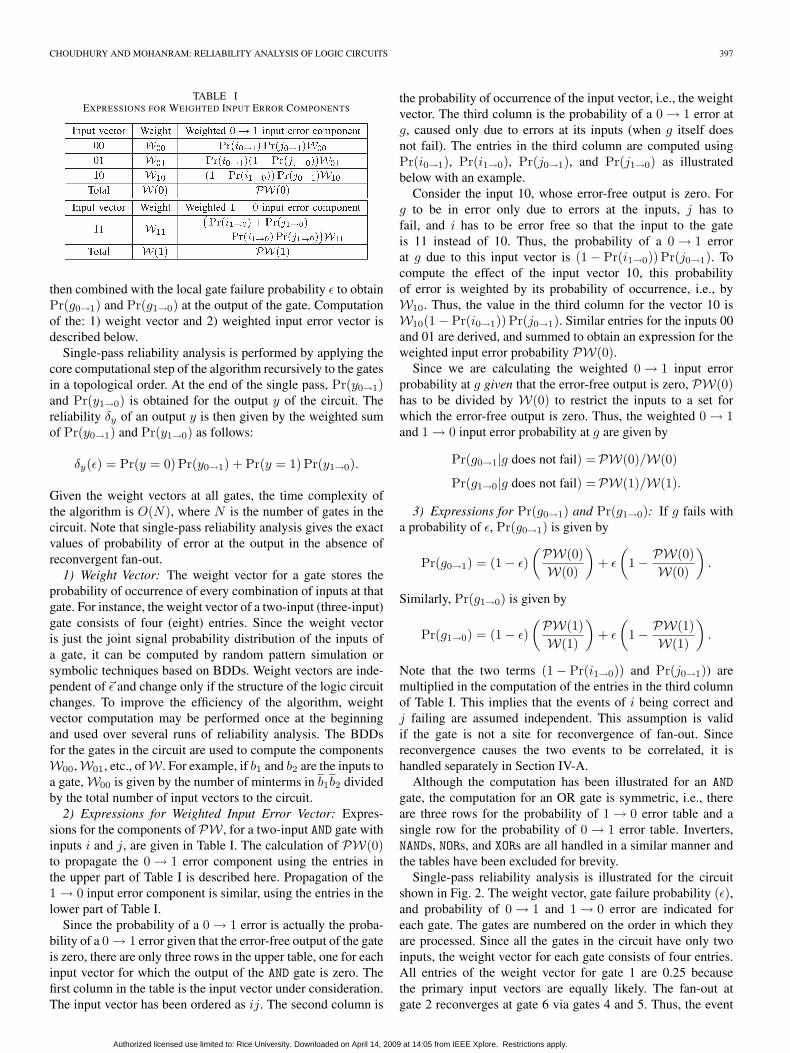
Single-pass reliability analysis is illustrated for the circuitshown in Fig. 2. The weight vector, gate failure probability (ε),and probability of 0 → 1 and 1 → 0 error are indicated foreach gate. The gates are numbered on the order in which theyare processed. Since all the gates in the circuit have only twoinputs, the weight vector for each gate consists of four entries.All entries of the weight vector for gate 1 are 0.25 becausethe primary input vectors are equally likely. The fan-out atgate 2 reconverges at gate 6 via gates 4 and 5. Thus, the event



Fig. 2. Illustrative example for single-pass reliability analysis.

of 0 → 1 and 1 → 0 error at the outputs of gates 4 and 5are correlated. However, independence is assumed and theprobability of these events are used in the computation of 0 → 1and 1 → 0 probability of error values for the output of gate 6.

A. Handling Reconvergent Fan-out

The presence of reconvergent fan-out renders the single-passreliability analysis approximate because the events of 0 → 1 or1 → 0 error for the inputs of a gate may not be independentat the point of reconvergence. Handling reconvergent fan-outhas been the subject of extensive research in signal probabilitycomputation. In this section, the theory of correlation coeffi-cients used in signal probability computation [21], is extendedto make single-pass reliability analysis more accurate in thepresence of reconvergent fan-out.

This approach relies on the propagation of the correlationcoefficients for a pair of wires from the source of fan-out tothe point of reconvergence. Note that the word “wire” hasbeen used as opposed to “node” because for a gate with fan-out > 1, each fan-out is treated as a separate wire, but theyconstitute the same node. The correlation coefficient for eventson a pair of wires is defined as the joint probability of the eventsdivided by the product of their marginal probabilities. Forsignal probability computation, an event on a wire is definedas the value of the wire being one. Thus, for a pair of wires, asingle correlation coefficient is sufficient to compute the jointprobability of a one on both the wires.

For reliability analysis, however, an event is defined as a0 → 1 or 1 → 0 error on a wire. Hence, instead of a singlecorrelation coefficient, four correlation coefficients for a pairof wires, one for every combination of events on the pair ofwires are used. If v and w are two wires, the four correlationcoefficients for this pair are denoted by Cvw, Cvw, Cvw, and Cvw,where v, w, v, and w refers to the event of a 0 → 1, 0 → 1,1 → 0, and 1 → 0 error at v and w, respectively.

The correlation coefficients come into play at the gates whoseinputs are the site of reconvergence of fan-out. At such gates,the events of 0 → 1 or 1 → 0 error at the inputs are notindependent. Thus, the entries in the third column of Table Iare weighted by the appropriate correlation coefficient, e.g.,Pr(i0→1)(1−Pr(j1→0)) becomes Pr(i0→1)(1−Pr(j1→0)Cij).

1) Correlation Coefficient Computation: The correlationcoefficient for a pair of wires can be calculated by first com-

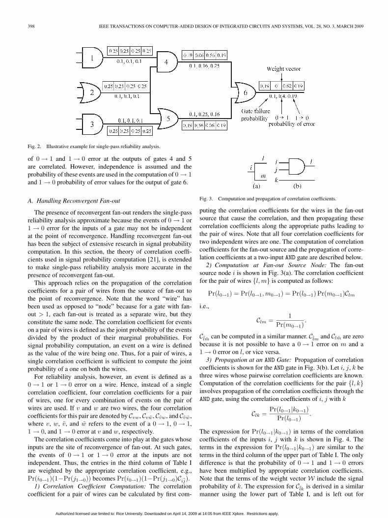
Fig. 3. Computation and propagation of correlation coefficients.

puting the correlation coefficients for the wires in the fan-outsource that cause the correlation, and then propagating thesecorrelation coefficients along the appropriate paths leading tothe pair of wires. Note that all four correlation coefficients fortwo independent wires are one. The computation of correlationcoefficients for the fan-out source and the propagation of corre-lation coefficients at a two-input AND gate are described below.

2) Computation at Fan-out Source Node: The fan-outsource node i is shown in Fig. 3(a). The correlation coefficientfor the pair of wires {l,m} is computed as follows:

Pr(l0→1) = Pr(l0→1,m0→1) = Pr(l0→1) Pr(m0→1)Clm

i.e.,

Clm =1

Pr(m0→1).

Clm can be computed in a similar manner. Clm and Clm are zerobecause it is not possible to have a 0 → 1 error on m and a1 → 0 error on l, or vice versa.

3) Propagation at an AND Gate: Propagation of correlationcoefficients is shown for the AND gate in Fig. 3(b). Let i, j, k bethree wires whose pairwise correlation coefficients are known.Computation of the correlation coefficients for the pair {l, k}involves propagation of the correlation coefficients through theAND gate, using the correlation coefficients of i, j with k

Clk =Pr(l0→1|k0→1)

Pr(l0→1).

The expression for Pr(l0→1|k0→1) in terms of the correlationcoefficients of the inputs i, j with k is shown in Fig. 4. Theterms in the expression for Pr(l0→1|k0→1) are similar to theterms in the third column of the upper part of Table I. The onlydifference is that the probability of 0 → 1 and 1 → 0 errorshave been multiplied by appropriate correlation coefficients.Note that the terms of the weight vector W include the signalprobability of k. The expression for Clk is derived in a similarmanner using the lower part of Table I, and is left out for



Fig. 4. Derivation of Pr(l0→1|k0→1) in terms of correlation coefficients of its inputs.

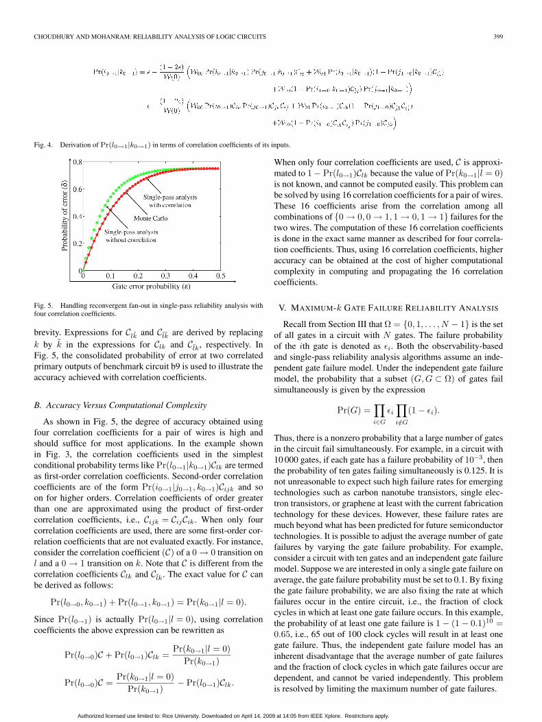
Fig. 5. Handling reconvergent fan-out in single-pass reliability analysis withfour correlation coefficients.

brevity. Expressions for Clk and Clk are derived by replacingk by k in the expressions for Clk and Clk, respectively. InFig. 5, the consolidated probability of error at two correlatedprimary outputs of benchmark circuit b9 is used to illustrate theaccuracy achieved with correlation coefficients.

B. Accuracy Versus Computational Complexity

As shown in Fig. 5, the degree of accuracy obtained usingfour correlation coefficients for a pair of wires is high andshould suffice for most applications. In the example shownin Fig. 3, the correlation coefficients used in the simplestconditional probability terms like Pr(l0→1|k0→1)Clk are termedas first-order correlation coefficients. Second-order correlationcoefficients are of the form Pr(i0→1|j0→1, k0→1)Cijk and soon for higher orders. Correlation coefficients of order greaterthan one are approximated using the product of first-ordercorrelation coefficients, i.e., Cijk = CijCik. When only fourcorrelation coefficients are used, there are some first-order cor-relation coefficients that are not evaluated exactly. For instance,consider the correlation coefficient (C) of a 0 → 0 transition onl and a 0 → 1 transition on k. Note that C is different from thecorrelation coefficients Clk and Clk. The exact value for C canbe derived as follows:

Pr(l0→0, k0→1) + Pr(l0→1, k0→1) = Pr(k0→1|l = 0).

Since Pr(l0→1) is actually Pr(l0→1|l = 0), using correlationcoefficients the above expression can be rewritten as

Pr(l0→0)C + Pr(l0→1)Clk =Pr(k0→1|l = 0)

Pr(k0→1)

Pr(l0→0)C =Pr(k0→1|l = 0)

Pr(k0→1)− Pr(l0→1)Clk.

When only four correlation coefficients are used, C is approxi-mated to 1 − Pr(l0→1)Clk because the value of Pr(k0→1|l = 0)is not known, and cannot be computed easily. This problem canbe solved by using 16 correlation coefficients for a pair of wires.These 16 coefficients arise from the correlation among allcombinations of {0 → 0, 0 → 1, 1 → 0, 1 → 1} failures for thetwo wires. The computation of these 16 correlation coefficientsis done in the exact same manner as described for four correla-tion coefficients. Thus, using 16 correlation coefficients, higheraccuracy can be obtained at the cost of higher computationalcomplexity in computing and propagating the 16 correlationcoefficients.

V. MAXIMUM-k GATE FAILURE RELIABILITY ANALYSIS

Recall from Section III that Ω = {0, 1, . . . , N − 1} is the setof all gates in a circuit with N gates. The failure probabilityof the ith gate is denoted as εi. Both the observability-basedand single-pass reliability analysis algorithms assume an inde-pendent gate failure model. Under the independent gate failuremodel, the probability that a subset (G,G ⊂ Ω) of gates failsimultaneously is given by the expression

Pr(G) =∏i∈G

εi

∏i/∈G

(1 − εi).

Thus, there is a nonzero probability that a large number of gatesin the circuit fail simultaneously. For example, in a circuit with10 000 gates, if each gate has a failure probability of 10−3, thenthe probability of ten gates failing simultaneously is 0.125. It isnot unreasonable to expect such high failure rates for emergingtechnologies such as carbon nanotube transistors, single elec-tron transistors, or graphene at least with the current fabricationtechnology for these devices. However, these failure rates aremuch beyond what has been predicted for future semiconductortechnologies. It is possible to adjust the average number of gatefailures by varying the gate failure probability. For example,consider a circuit with ten gates and an independent gate failuremodel. Suppose we are interested in only a single gate failure onaverage, the gate failure probability must be set to 0.1. By fixingthe gate failure probability, we are also fixing the rate at whichfailures occur in the entire circuit, i.e., the fraction of clockcycles in which at least one gate failure occurs. In this example,the probability of at least one gate failure is 1 − (1 − 0.1)10 =0.65, i.e., 65 out of 100 clock cycles will result in at least onegate failure. Thus, the independent gate failure model has aninherent disadvantage that the average number of gate failuresand the fraction of clock cycles in which gate failures occur aredependent, and cannot be varied independently. This problemis resolved by limiting the maximum number of gate failures.



If we are concerned with only single gate failures, we canset the limit to one. Now, the failure probability of the gateswill determine the fraction of clock cycles in which at least onegate failure occurs in the circuit. For instance, if the failureprobability is 0.1, the probability that no gate failures occuris equal to (1 − 0.1)10 = 0.910. Probability that exactly onegate fails is 10 × 0.1 × (1 − 0.1)9 = 0.99. Hence, the fractionof clock cycles in which gate failures occur is 0.99/(0.910 +0.99) = 0.53. Single-event upsets are an excellent example ofmaximum-k gate failure model. For instance, let us assume thatthe flux of energetic particle strikes is such that it can cause oneupset every N cycles. In the maximum-k gate failure model,this is done by setting the limit on the number of gate failuresto one, and adjusting the failure probabilities of the gates suchthat the error rate of the circuit is 1/N . To summarize, a morerealistic gate failure model is to have an upper bound on thenumber of simultaneous gate failures.

Under the maximum-k gate failure model, gate failures arestill independent of each other. However, an additional con-straint, that only a maximum of k gates can fail simultaneously,is introduced. This global constraint causes the gate failures tobe correlated with each other, which can be explained mathe-matically as follows. Note that the maximum number of gatefailures that can occur in parallel is an empirical quantity thatdepends on the source of the noise. For instance, in the caseof memories, single/double bit errors are pervasive. A similarcharacterization of noise sources in logic circuits can be usedto determine the maximum simultaneous number of failures ina logic circuit.

Let Xi be a random variable that takes a value one whenthe ith gate fails and a value zero otherwise. In the maximum-k gate failure model, the Xis are independent of each other,but the additional constraint is that

∑Xi ≤ k. This constraint

means that Pr(Xk+1 = 1|X1 = 1,X2 = 1, . . . , Xk = 1) = 0.However, Pr(Xk+1 = 1) = εk+1. Since the conditional proba-bility is not equal to the marginal probability, the gate failuresare correlated with each other.

In the rest of this section, a maximum-k gate failure reliabil-ity analysis algorithm that combines a sampling algorithm withsingle-pass reliability analysis is described. Several techniquesto sample k (with given weights) out of a sample space of Nhave been proposed in literature, e.g., [22]. However, for themaximum-k gate failure model, the size of the sample space is(N0

)+(N1

)+ · · · + (Nk ). For N of the order of 104, the sample

space becomes intractably large even for k = 3. However, aspecial property of the sample space—the independence of gatefailures—is exploited in the proposed sampling algorithm toreduce the computational complexity to O(Nk2).

A. Why Fault Injection and Simulation Does Not Scale

The most straightforward algorithm for reliability analysiswith the maximum-k gate failure model is based on fault in-jection and random pattern simulation in a Monte Carlo frame-work. By generating a random number uniformly distributedover the interval [0,1] for each gate and comparing it to thefailure probability of the gate, it can be determined whetherthe gate has failed or not. Thus, the set of all failed gates

constitutes a sample of failed gates. Since the random numbersfor each gate are generated independently, there is no controlover the size of the sample. A sample of failed gates has to bediscarded if it violates the constraint on the maximum numberof gate failures. If the constraint is satisfied, random patternsimulation is performed to evaluate the effect of the failed gateson the outputs. This procedure is repeated for a large number ofsamples, and their effect on the outputs is averaged.

A major drawback of this algorithm is that for large valuesof gate failure probabilities and low values of k, a large numberof generated samples may not obey the constraint on maximumnumber of gate failures and have to be discarded. For instance,suppose that the total number of gates in the circuit is 10 000,each gate fails independently with a probability 0.05, and k=3.Since fault injection is performed independently at each gate,the average number of erroneous gates is 10 000 × 0.05 =500 3. Hence, a large number of samples will be discardedbecause they do not satisfy the constraint on the maximumnumber of gate failures. Thus, a very large number of runs arerequired to achieve convergence of the solution, and this makesthe algorithm computationally intensive.

In contrast, the maximum-k gate failure algorithm, describedbelow, is based on generating only correct samples of gatefailures (which satisfy the constraint on the maximum numberof gate failures). After generating a sample of failed gates, thesingle-pass reliability analysis algorithm is used to evaluate theprobability of error at the output of the circuit. The probabilityof failure at each primary output is obtained by averaging overa large number of samples. Since only correct samples aregenerated and since single-pass reliability analysis is used tocompute the effect of each sample of gate failures, the algorithmis orders of magnitude faster the Monte Carlo approach.

B. Sampling Algorithm

When the maximum number of simultaneous gate failures isbounded by k, the sample space of the possible combinationsof simultaneous gate failures is reduced to sets G with |G| ≤ k.Let Sε be the sum of the probability of gate failure combina-tions in this sample space. Thus, Sε is given by the followingexpression:

Sε =∑

{G⊂Ω,|G|≤k}

∏i∈G

εi

∏i/∈G

(1 − εi).

Note that Sε �= 1 because the sample space is reduced to sets Gsuch that |G| ≤ k. Thus, for the maximum-k gate failure modelthe probability that a subset of gates, G, fail simultaneously isgiven by the following expression:

Pr(G) ={∏

i∈G εi

∏i/∈G(1 − εi)/Sε, |G| ≤ k

0, |G| > k.(3)

Let αi = εi/(1 − εi). If Sα is defined as

Sα =∑

{G⊂Ω,|G|≤k}

∏i∈G

αi



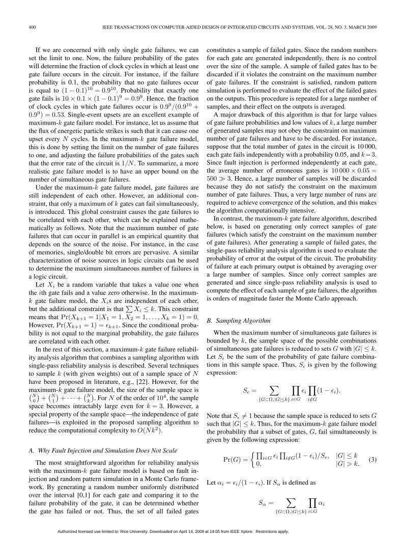
TABLE IISAMPLE SPACE OF POSSIBLE GATE FAILURES

(3) can be rewritten more succinctly in terms of αi and Sα as

Pr(G) ={∏

i∈G αi/Sα, |G| ≤ k0, |G| > k.

(4)

As an illustration for the probability distribution expressed by(4), the sample space and associated probability of failure forN = 4 and k = 2 is shown in Table II.

We start by describing two straightforward techniques forgenerating samples of erroneous gates according to the proba-bility distribution given in (3). It turns out that the first solutionis incorrect because the generated samples have a slightlydifferent probability distribution, and that the second solution iscomputationally intractable. This motivates the third solution,which is efficient and generates the samples from the correctprobability distribution.

The first intuitive approach to generate a sample of ≤ k gatesis to select the gates one at a time over k steps. In each step,the interval [0,1] is divided into subintervals proportional to{1, α1, α2, . . .}. The subinterval αi corresponds to failure ofgate i. The subinterval proportional to one corresponds to “nogate failure.” A uniformly distributed random number is gener-ated in the interval [0,1] and the subinterval in which the gener-ated random number lies indicates the erroneous gate. Note thatif the random number lies in the subinterval proportional to one,then no gate is erroneous in that step. If the random number liesin the interval αi, then the ith gate is designated as failed, and itis removed from the Ω. The reduced Ω is then used for the nextstep. This procedure is repeated for k steps. For instance, sup-pose k = 3. If the three steps generate {1, 1, 1}, then no gate hasfailed (denoted as {} in Table II). If {1, α2, α4} is generated,then gate 2 and gate 4 have failed (denoted as {2, 4} in Table II).Although this approach seems correct at first, a closer look re-veals that the distribution from which the sample of failed gatesis generated by this approach is incorrect. The reason is that thesamples of gate failures shown in Table II are unordered sets,i.e., the sample {1, α2, α4} is the same as {α2, 1, α4}. How-ever, the sample {α1, α2, α4} can be generated in six ways inthis algorithm (differing only in the order in which the gates aregenerated in different steps, {α1, α2, α4}, {α1, α4, α2}, . . .).However, the sample {1, 1, 1} can be generated only once, andthe sample {1, 1, α2} can be generated in only three ways.

A second straightforward but inefficient approach is to dividethe interval [0,1] into subintervals of widths equal to the proba-

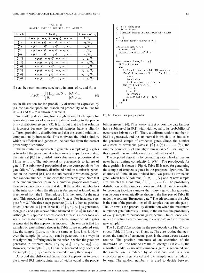
Fig. 6. Proposed sampling algorithm.

bilities given in (4). Thus, every subset of possible gate failureshas a subinterval in [0,1] with width equal to its probability ofoccurrence [given by (4)]. Then, a uniform random number in[0,1] is generated, and the subinterval in which it lies indicatesthe generated sample of erroneous gates. Since, the numberof subsets of erroneous gates is

(N0

)+(N1

)+ · · · + (Nk ), the

runtime complexity of this algorithm is O(Nk). For large N ,this algorithm is unusable even for small values of k.

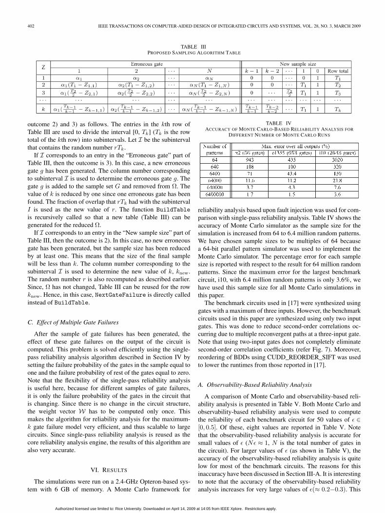
The proposed algorithm for generating a sample of erroneousgates has a runtime complexity O(Nk2). The pseudocode forthe algorithm is shown in Fig. 6. Table III is used for generatingthe sample of erroneous gates in the proposed algorithm. Thecolumns of Table III are divided into two parts: 1) erroneousgate, which has N columns, {1, 2, . . . , N} and 2) new samplesize, which has k columns, {0, 1, . . . , k − 1}. The probabilitydistribution of the samples shown in Table II can be rewrittenby grouping together samples that share a gate. This groupingcan be done systematically as shown in the first part of Table IIIunder the column “Erroneous gate.” The jth column in the tableis the sum of the probabilities of all samples that contain gate j.The ith row is the probability distribution when the maximumnumber of gate failures is i. Thus, in the ith row, the probabilityof every sample of erroneous gates occurs i times, once eachunder the column corresponding to every gate in the erroneousgate sample.

The BuildTable routine in the pseudocode (in Fig. 6) con-structs Table III for a given Ω and k. The core routine that gen-erates the sample of erroneous gates is the NextGateFailureroutine. The possible outcomes of an execution of theNextGateFailure routine are the following: 1) if k = 0, thealgorithm ends; 2) no new erroneous gate is generated andthe sample size is reduced by at least one; and 3) a newerroneous gate is generated and the sample size is reducedby one. The random number r is used to decide between



TABLE IIIPROPOSED SAMPLING ALGORITHM TABLE

outcome 2) and 3) as follows. The entries in the kth row ofTable III are used to divide the interval [0, Tk] (Tk is the rowtotal of the kth row) into subintervals. Let I be the subintervalthat contains the random number rTk.

If I corresponds to an entry in the “Erroneous gate” part ofTable III, then the outcome is 3). In this case, a new erroneousgate g has been generated. The column number correspondingto subinterval I is used to determine the erroneous gate g. Thegate g is added to the sample set G and removed from Ω. Thevalue of k is reduced by one since one erroneous gate has beenfound. The fraction of overlap that rTk had with the subintervalI is used as the new value of r. The function BuildTableis recursively called so that a new table (Table III) can begenerated for the reduced Ω.

If I corresponds to an entry in the “New sample size” part ofTable III, then the outcome is 2). In this case, no new erroneousgate has been generated, but the sample size has been reducedby at least one. This means that the size of the final samplewill be less than k. The column number corresponding to thesubinterval I is used to determine the new value of k, knew.The random number r is also recomputed as described earlier.Since, Ω has not changed, Table III can be reused for the rowknew. Hence, in this case, NextGateFailure is directly calledinstead of BuildTable.

C. Effect of Multiple Gate Failures

After the sample of gate failures has been generated, theeffect of these gate failures on the output of the circuit iscomputed. This problem is solved efficiently using the single-pass reliability analysis algorithm described in Section IV bysetting the failure probability of the gates in the sample equal toone and the failure probability of rest of the gates equal to zero.Note that the flexibility of the single-pass reliability analysisis useful here, because for different samples of gate failures,it is only the failure probability of the gates in the circuit thatis changing. Since there is no change in the circuit structure,the weight vector W has to be computed only once. Thismakes the algorithm for reliability analysis for the maximum-k gate failure model very efficient, and thus scalable to largecircuits. Since single-pass reliability analysis is reused as thecore reliability analysis engine, the results of this algorithm arealso very accurate.

VI. RESULTS

The simulations were run on a 2.4-GHz Opteron-based sys-tem with 6 GB of memory. A Monte Carlo framework for

TABLE IVACCURACY OF MONTE CARLO-BASED RELIABILITY ANALYSIS FOR

DIFFERENT NUMBER OF MONTE CARLO RUNS

reliability analysis based upon fault injection was used for com-parison with single-pass reliability analysis. Table IV shows theaccuracy of Monte Carlo simulator as the sample size for thesimulation is increased from 64 to 6.4 million random patterns.We have chosen sample sizes to be multiples of 64 becausea 64-bit parallel pattern simulator was used to implement theMonte Carlo simulator. The percentage error for each samplesize is reported with respect to the result for 64 million randompatterns. Since the maximum error for the largest benchmarkcircuit, i10, with 6.4 million random patterns is only 3.6%, wehave used this sample size for all Monte Carlo simulations inthis paper.

The benchmark circuits used in [17] were synthesized usinggates with a maximum of three inputs. However, the benchmarkcircuits used in this paper are synthesized using only two inputgates. This was done to reduce second-order correlations oc-curring due to multiple reconvergent paths at a three-input gate.Note that using two-input gates does not completely eliminatesecond-order correlation coefficients (refer Fig. 7). Moreover,reordering of BDDs using CUDD_REORDER_SIFT was usedto lower the runtimes from those reported in [17].

A. Observability-Based Reliability Analysis

A comparison of Monte Carlo and observability-based reli-ability analysis is presented in Table V. Both Monte Carlo andobservability-based reliability analysis were used to computethe reliability of each benchmark circuit for 50 values of ε ∈[0, 0.5]. Of these, eight values are reported in Table V. Notethat the observability-based reliability analysis is accurate forsmall values of ε (Nε ≈ 1, N is the total number of gates inthe circuit). For larger values of ε (as shown in Table V), theaccuracy of the observability-based reliability analysis is quitelow for most of the benchmark circuits. The reasons for thisinaccuracy have been discussed in Section III-A. It is interestingto note that the accuracy of the observability-based reliabilityanalysis increases for very large values of ε(≈ 0.2−0.3). This



Fig. 7. Figure shows the circuit structures that introduce (a) first-order and(b) higher-order correlation coefficients.

is because for such large values of ε, δ(ε) for the outputs beginto saturate at 0.5 (pure noise). The value of the observability-based closed-form expression also begins to saturate to 0.5for those values of ε. Hence, the percentage error decreases.When ε is 0.5, both evaluate to 0.5 and the percentage erroris zero. The runtimes for small- and medium-sized circuits areencouraging. However, for the large benchmark circuits (e.g.,c3540) the runtime is high. This is because exact observabilitycomputation is computationally intensive as reconvergent fan-out increases, and this occurs with the c3540 benchmark.

B. Single-Pass Reliability Analysis

Simulation results comparing single-pass reliability analysiswith Monte Carlo simulations are reported in Table VI. InTable VI, columns 1 and 2 give the name and number of gatesin the benchmark circuit. Both the Monte Carlo and single-pass reliability frameworks were used to compute δ(�ε) for tendifferent values of ε over the range 0 to 0.5. Note that thesame value of ε has been used for all the gates in the circuit,and hence, �ε is replaced by ε. The third column reports thepercentage error in single-pass reliability analysis with 0, 4, and16 correlation coefficients, averaged over all the outputs andover ten values of ε ∈ [0, 0.5]. The cumulative runtime for tenruns is reported in the fourth column. The runtime required forthe weight vector computation used in the single-pass reliabilityanalysis is reported under the setup time column in the table.

The maximum percentage error in δ(�ε) is less than 2%for the largest benchmark circuit, i10. For circuits with sig-nificant reconvergent fan-out, e.g., c499, c1355, and c1908,the maximum percentage error in δ(�ε) is 13.1%, 13.5%, and

6.5%, respectively. The largest percentage error is observedwhen zero correlation coefficients are used, i.e., when thecorrelations in failures introduced due to reconvergent fan-out is ignored. The percentage error progressively improvesas 4 and 16 correlation coefficients are used. Note that theerror correcting benchmark circuits like c499, c1355, andc1908 have large reconvergent fan-out that requires the useof higher-order correlation coefficients. The circuit structure(s)that introduce first-order and higher-order correlation coeffi-cients are shown in Fig. 7(a) and (b) respectively. Since thehigher-order correlation coefficients are approximated in allthree schemes (0, 4, and 16), only a slight improvement inaccuracy is observed when 4 and 16 correlation coefficientsare used.

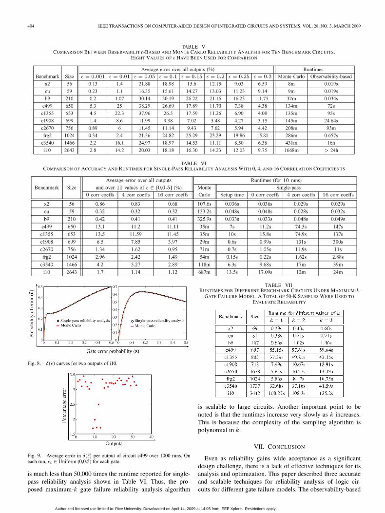
Fig. 8 shows δ(ε) for two outputs of benchmark i10. The conesizes of the two outputs are 662 and 1034 gates, respectively.Each graph has two curves: one from Monte Carlo reliabilityanalysis and one from single-pass reliability analysis using zerocorrelation coefficients. The two curves are indistinguishable,as shown in the figure. The diverse shapes of the curvesillustrates not only the complexity of the relation between δ andε, but also the accuracy of single-pass reliability analysis.

Fig. 9 shows the percentage error in δ(�ε) for each of the32 outputs of benchmark circuit c499. On each run, the ε foreach gate was derived from a uniform random distributionover the interval [0,0.5]. Single-pass reliability analysis withzero correlation coefficients was compared to Monte Carloreliability analysis. The percentage error in δ(�ε) for each output,averaged over 1000 runs, is 1.5%–3.5%. This illustrates thatsingle-pass reliability analysis is highly accurate even when theε values are allowed to vary independently at every gate.

It is clear from the results that the proposed single-pass relia-bility analysis technique is highly accurate. Although a head-to-head performance comparison with approaches based onPTMs and Bayesian networks was not possible, it is our beliefbased on the results reported in [9] that the proposed techniqueaffords at least a 500 X speedup over Bayesian networks onthe largest circuit b9: 2.5 seconds for Bayesian networks versus0.005 seconds per run with single-pass reliability analysis. Notealso that results reported in [9] show that Bayesian networksafford a 1000 X speedup over PTMs. In summary, it is rea-sonable to conclude that the strengths of the proposed single-pass reliability analysis algorithm are its accuracy, scalabilityto large circuits, and speedup in performance.

C. Maximum-k Gate Failure Model

The results for reliability analysis under the maximum-kgate failure model for different benchmark circuits is shown inTable VII. The results have been presented for three values ofk. Single-pass reliability analysis with zero correlation coeffi-cients was used as the core engine to evaluate the reliabilityfor the 50,000 samples generated by the sampling algorithm.A significant fraction of the runtime can be attributed to theweight vector computation W . For the maximum-k gate failurereliability analysis, W is computed only once and stored foruse in all the 50,000 runs. Thus, the runtime reported formaximum-k gate failure reliability analysis shown in Table VII



TABLE VCOMPARISON BETWEEN OBSERVABILITY-BASED AND MONTE CARLO RELIABILITY ANALYSIS FOR TEN BENCHMARK CIRCUITS.

EIGHT VALUES OF ε HAVE BEEN USED FOR COMPARISON

TABLE VICOMPARISON OF ACCURACY AND RUNTIMES FOR SINGLE-PASS RELIABILITY ANALYSIS WITH 0, 4, AND 16 CORRELATION COEFFICIENTS

Fig. 8. δ(ε) curves for two outputs of i10.

Fig. 9. Average error in δ(�ε) per output of circuit c499 over 1000 runs. Oneach run, εi ∈ Uniform (0,0.5) for each gate.

is much less than 50,000 times the runtime reported for single-pass reliability analysis shown in Table VI. Thus, the pro-posed maximum-k gate failure reliability analysis algorithm

TABLE VIIRUNTIMES FOR DIFFERENT BENCHMARK CIRCUITS UNDER MAXIMUM-k

GATE FAILURE MODEL. A TOTAL OF 50-K SAMPLES WERE USED TO

EVALUATE RELIABILITY

is scalable to large circuits. Another important point to benoted is that the runtimes increase very slowly as k increases.This is because the complexity of the sampling algorithm ispolynomial in k.

VII. CONCLUSION

Even as reliability gains wide acceptance as a significantdesign challenge, there is a lack of effective techniques for itsanalysis and optimization. This paper described three accurateand scalable techniques for reliability analysis of logic cir-cuits for different gate failure models. The observability-based



reliability analysis algorithm provides a closed-form expressionfor reliability using the observabilities of the gates, and isaccurate when single gate failures are dominant. The single-pass reliability analysis algorithm is based on a single topo-logical walk through the circuit to compute the reliability ofthe circuit, and is accurate even for multiple gate failures. Themaximum-k gate failure reliability analysis algorithm allows anupper limit, k, on the number of simultaneous gate failures in acircuit. An efficient sampling technique is proposed to generatea set of ≤ k failed gates, and single-pass reliability analysis isused to evaluate the effect of these failed gates at the outputs.The three algorithms have potential applications to reliabilityanalysis of failures arising due to a broad range of mechanismsincluding single-event effects, process variations, and reliabilitydegradation due to aging.

REFERENCES

[1] R. W. Keyes, “Fundamental limits of silicon technology,” Proc. IEEE,vol. 89, no. 3, pp. 227–239, Mar. 2001.

[2] J. D. Meindl, Q. Chen, and J. A. Davis, “Limits on silicon nanoelectronicsfor terascale integration,” Science, vol. 293, no. 5537, pp. 2044–2049,Sep. 2001.

[3] G. Bourianoff, “The future of nanocomputing,” Computer, vol. 36, no. 8,pp. 44–53, Aug. 2003.

[4] V. V. Zhirnov, R. K. Cavin, J. A. Hutchby, and G. I. Bourianoff, “Limitsto binary logic switch scaling—A Gedanken model,” Proc. IEEE, vol. 91,no. 11, pp. 1934–1939, Nov. 2003.

[5] M. A. Breuer, S. K. Gupta, and T. M. Mak, “Defect and error tolerancein the presence of massive numbers of defects,” IEEE Des. Test Comput.,vol. 21, no. 3, pp. 216–227, May/Jun. 2004.

[6] J. von Neumann, “Probabilistic logics and the synthesis of reli-able organisms from unreliable components,” in Automata Studies,C. E. Shannon and J. McCarthy, Eds. Princeton, NJ: Princeton Univ.Press, 1956, pp. 43–98.

[7] A. Sadek, K. Nikoliæ, and M. Forshaw, “Parallel information and com-putation with restitution for noise-tolerant nanoscale logic networks,”Nanotechnology, vol. 15, no. 1, pp. 192–210, Jan. 2004.

[8] S. Krishnaswamy, G. Viamontes, I. Markov, and J. Hayes, “Accurate re-liability evaluation and enhancement via probabilistic transfer matrices,”in Proc. Des. Autom. Test Eur., 2005, pp. 282–287.

[9] T. Rejimon and S. Bhanja, “Scalable probabilistic computing modelsusing Bayesian networks,” in Proc. Int. Midwest Symp. Circuits Syst.,2005, pp. 712–715.

[10] I. Bahar, J. L. Mundy, and J. Chen, “A probabilistic-based design method-ology for nanoscale computation,” in Proc. Int. Conf. Comput.-AidedDes., 2003, pp. 480–486.

[11] D. Bhaduri and S. Shukla, “Nanolab: A tool for evaluating reliabilityof defect-tolerant nano architectures,” in Proc. Annu. Symp. VLSI, 2004,pp. 25–31.

[12] B. Zhang, W.-S. Wang, and M. Orshansky, “FASER: Fast analysis of softerror susceptibility for cell-based designs,” in Proc. Int. Symp. QualityElectron. Des., 2006, pp. 755–760.

[13] M. Zhang and N. R. Shanbhag, “A soft error rate analysis (SERA) method-ology,” in Proc. Int. Conf. Comput.-Aided Des., 2004, pp. 111–118.

[14] S. Almukhaizim, Y. Makris, Y.-S. Yang, and A. Veneris, “Seamless inte-gration of SER in rewiring based design space exploration,” in Proc. Int.Test Conf., 2006, pp. 1–9.

[15] S. Krishnaswamy, S. Plaza, I. Markov, and J. Hayes, “Enhancing designrobustness with reliability-aware resynthesis and logic simulation,” inProc. Int. Conf. Comput.-Aided Des., 2007, pp. 149–154.

[16] M. Choudhury and K. Mohanram, “Approximate logic circuits for lowoverhead, non-intrusive concurrent error detection,” in Proc. Des. Autom.Test Eur., 2008, pp. 903–908.

[17] M. Choudhury and K. Mohanram, “Accurate and scalablereliability analysis of logic circuits,” in Proc. Des. Autom. Test Eur., 2007,pp. 1454–1459.

[18] M. Nemani and F. Najm, “Towards a high-level power estimation capa-bility,” IEEE Trans. Comput.-Aided Design Integr. Circuits Syst., vol. 15,no. 6, pp. 588–598, Jun. 1996.

[19] M. Damiani and G. De Micheli, “Observability don’t care sets andBoolean relations,” in Proc. Int. Conf. Comput.-Aided Des., 1990,pp. 502–505.

[20] T. Larrabee, “Test pattern generation using Boolean satisfiability,”IEEE Trans. Comput.-Aided Design Integr. Circuits Syst., vol. 11, no. 1,pp. 4–15, Jan. 1992.

[21] S. Ercolani, M. Favalli, M. Damiani, P. Olivo, and B. Ricco, “Estimateof signal probability in combinational logic networks,” in Proc. Eur. TestConf., 1989, pp. 132–138.

[22] G. Fishman, “Monte Carlo: Concepts, algorithms and applications,” inSpringer Series in Operations Research. New York: Springer-Verlag,1995.

Mihir R. Choudhury (S’06) received the B.Tech.degree in computer science and engineering fromIndian Institute of Technology, Bombay, India, in2005 and the M.S. degree in electrical and computerengineering from Rice University, Houston, TX, in2008, where he is currently working toward the Ph.D.degree in computer engineering.

His research interests include logic synthesis, cir-cuit simulation, and design for reliability in scaledelectronic technologies.

Kartik Mohanram (S’00–M’04) received theB.Tech. degree in electrical engineering from IndianInstitute of Technology, Bombay, India, in 1998 andthe M.S. and Ph.D. degrees in computer engineeringfrom University of Texas, Austin, in 2000 and 2003,respectively.

He is currently an Assistant Professor with theDepartment of Electrical and Computer Engineering,Rice University, Houston, TX. His primary researchinterests are in computer engineering and systems,with an emphasis on modeling, simulation, and

computer-aided design for scaled electronic technologies.Dr. Mohanram is a recipient of the National Science Foundation CAREER

Award, the Association for Computing Machinery/Special Interest Group De-sign Automation Technical Leadership Award, and the A. Richard NewtonGraduate Scholarship.


Reliability Analysis of Logic Circuitskmram/publications/tcad09.pdfDigital Object Identiﬁer...

Documents

Transcript of Reliability Analysis of Logic Circuitskmram/publications/tcad09.pdfDigital Object Identiﬁer...