On the False Discovery Rates of a Frequentist: Asymptotic ...

On the False Discovery Rates of a

Frequentist: Asymptotic Expansions

Anirban DasGupta

Department of Statistics, Purdue University105 North University Street

West Lafayette, IN 47907-2067email: [email protected]

Tonglin Zhang

Department of Statistics, Purdue University105 North University Street

West Lafayette, IN 47907-2067email: [email protected]

Abstract: Consider a testing problem for the null hypothesis H0 : θ ∈ Θ0.The standard frequentist practice is to reject the null hypothesis when thep-value is smaller than a threshold value α, usually 0.05. We ask the ques-tion how many of the null hypotheses a frequentist rejects are actuallytrue. Precisely, we look at the Bayesian false discovery rate δn = Pg(θ ∈Θ0|p − value < α) under a proper prior density g(θ). This depends on theprior g, the sample size n, the threshold value α as well as the choice of thetest statistic. We show that the Benjamini-Hochberg FDR in fact convergesto δn almost surely under g for any fixed n. For one-sided null hypothe-ses, we derive a third order asymptotic expansion for δn in the continuousexponential family when the test statistic is the MLE and in the locationfamily when the test statistic is the sample median. We also briefly men-tion the expansion in the uniform family when the test statistic is the MLE.The expansions are derived by putting together Edgeworth expansions forthe CDF, Cornish-Fisher expansions for the quantile function and variousTaylor expansions. Numerical results show that the expansions are veryaccurate even for a small value of n (e.g., n = 10). We make many usefulconclusions from these expansions, and specifically that the frequentist isnot prone to false discoveries except when the prior g is too spiky. Theresults are illustrated by many examples.

AMS 2000 subject classifications: Primary 62F05; secondary 62F03,62F15.Keywords and phrases: Cornish-Fisher expansions, Edgeworth expan-sions, exponential families, false discovery rate, location families, MLE,p-value.

1. Introduction

In a strikingly interesting short note, Soric [19] raised the question of estab-lishing upper bounds on the proportion of fictitious statistical discoveries in abattery of independent experiments. Thus, if m null hypotheses are tested inde-pendently,of which m0 happen to be true, but V among these m0 are rejected

1

imsart ver. 2006/01/04 file: pvaluerev.tex date: April 9, 2006

2

at a significance level α, and another S among the false ones are also rejected,Soric essentially suggested E(V )/(V +S) as a measure of the false discovery ratein the chain of m independent experiments. Benjamini and Hochberg [3] thenlooked at the question in much greater detail and gave a careful discussion forwhat a correct formulation for the false discovery rate of a group of frequentistsshould be, and provided a concrete procedure that actually physically controlsthe groupwise false discovery rate. The problem is simultaneously theoreticallyattractive,socially relevant, and practically important. The practical importancecomes from its obvious relation to statistical discoveries made in clinical trials,and in modern microarray experiments. The continued importance of the prob-lem is reflected in two recent articles, Efron [5], and Storey [21], who provideserious Bayesian connections and advancements in the problem. See also Storey[20], Storey, Taylor and Siegmund [23], Storey and Tibshirani [22], Genoveseand Wasserman [10], and Finner and Roters [9], among many others in thiscurrently active area.

Around the same time that Soric raised the issue of fictitious frequentistdiscoveries made by a mechanical adoption of the use of p-values, a differentdebate was brewing in the foundation literature. Berger and Sellke [2], in athought provoking article, gave analytical foundations to the thesis in Edwards,Lindman and Savage [4] that the frequentist practice of rejecting a sharp null ata traditional 5% level amounts to a rush to judgment against the null hypothesis.By deriving lower bounds or exact values for the minimum value of the posteriorprobability of a sharp null hypothesis over a variety of classes of priors, Bergerand Sellke [2] argued that p-values traditionally regarded as small understatethe plausibility of nulls, at least in some problems. Casella and Berger [7], gavea collection of theorems that show that the discrepancy disappears under broadconditions if the null hypothesis is composite one-sided. Since the articles ofBerger and Sellke [2] and Casella and Berger [7], there has been an avalanche ofactivity in the foundation literature on the safety of use of p-values in testingproblems. See Hall and Sellinger [11], Sellke, Bayarri and Berger [18], Marden[14] and Schervish [17] for a contemporary exposition.

It is conceptually clear that the frequentist FDR literature and the foundationliterature were both talking about a similar issue : is the frequentist practice ofrejecting nulls at traditional p-values an invitation to rampant false discoveries? The structural difference was that the FDR literature did not introduce aformal prior on the unknown parameters, while the foundation literature didnot go into multiple testing, as is the case in microarray or other emerginginteresting applications. The purpose of this article is to marry the two schoolstogether, while giving a new rigorous analysis of the interesting question : “howmany of the null hypotheses a frequentist rejects are actually true” and the flipside of that question, namely, “how many of the null hypotheses a frequentistaccepts are actually false”. The calculations are completely different from whatthe previous researchers have done, although we then demonstrate that ourformulation directly relates to both the traditional FDR calculations, and thefoundational effort in Berger and Sellke [2], and others. We have thus a dual goal;providing a new approach, and integrating it with the two existing approaches.


3

In Section 2, we demonstrate the connection in very great generality, withoutpractically any structural assumptions at all. This was comforting. As regardsconcrete results, it seems appropriate that the one parameter exponential familycase be looked at, it being the first structured case one would want to investigate.In Section 3, we do so, using the MLE as the test statistic. In Section 4, we lookat a general location parameter, but using the median as the test statistic. Weused the median for two reasons. First, for general location parameters, themedian is credible as a test statistic, while the mean obviously is not. Second,it is important to investigate the extent to which the answers depend on thechoice of the test statistic; by studying the median, we get an opportunity tocompare the answers for the mean and the median in the special normal case.Tobe specific, let us consider the one sided testing problem based on an i.i.d. sampleX1, · · · ,Xn from a distribution family with parameter θ in the parameter spaceΩ which is an interval of R. Without loss of generality, we assume Ω = (θ, θ)with −∞ ≤ θ < θ ≤ ∞. We consider the testing problem

H0 : θ ≤ θ0 vs H1 : θ > θ0,

where θ0 ∈ (θ, θ). Suppose the α, 0 < α < 1, level test rejects H0 if Tn ∈ C,where Tn is a test statistic. We study the behavior of the quantities,

δn = P (θ ≤ θ0|Tn ∈ C) = P (H0|p − value < α)

andεn = P (θ > θ0|Tn 6∈ C) = P (H1|p − value ≥ α).

Note that δn and εn are inherently Bayesian quantities. By an almost egregiousabuse of nomenclature, we will refer to δn and εn as type I and type II errors inthis article. Our principal objective is to obtain third order asymptotic expan-sions for δn and εn assuming a Bayesian proper prior for θ. Suppose g(θ) is anysufficiently smooth proper prior density of θ. In the regular case, the expansionfor δn we obtain is like

δn =P (θ ≤ θ0, Tn ∈ C)

P (Tn ∈ C)=

c1√n

+c2

n+

c3

n3/2+ O(n−2), (1)

and the expansion for εn is like

εn =P (θ > θ0, Tn 6∈ C)

P (Tn 6∈ C)=

d1√n

+d2

n+

d3

n3/2+ O(n−2), (2)

where the coefficients c1, c2, c3, d1, d2, and d3 depend on the problem, the teststatistic Tn, the value of α and the prior density g(θ). In the nonregular case,the expansion differs qualitatively; for both δn and εn the successive terms arein powers of 1/n instead of the powers of 1/

√n. Our ability to derive a third

order expansion results in a surprisingly accurate expansion, sometimes for n assmall as n = 4. The asymptotic expansions we derive are not just of theoreticalinterest; the expansions let us conclude interesting things, as in Sections 3.2 and


4

4.5, that would be impossible to conclude from the exact expressions for δn andεn.

The expansions of δn and εn require the expansions of the numerators andthe denominators of (1) and (2) respectively. In the regular case, the expansionof the numerator of (1) is like

An = P (θ ≤ θ0, Tn ∈ C) =a1√n

+a2

n+

a3

n3/2+ O(n−2) (3)

and the expansion of the numerator of (2) is like

An = P (θ > θ0, Tn 6∈ C) =a1√n

+a2

n+

a3

n3/2+ O(n−2). (4)

Then, the expansion of the denominator of (1) is

Bn = P (Tn ∈ C) = An + λ − An = λ − b1√n− b2

n− b3

n3/2+ O(n−2), (5)

where λ = P (θ > θ0) =∫ θ

θ0g(θ)dθ and assume 0 < λ < 1, b1 = a1 − a1,

b2 = a2 − a2 and b3 = a3 − a3, and the expansion of the denominator of (2) is

Bn = P (Tn 6∈ C) = 1 − Bn = 1 − λ +b1√n

+b2

n+

b3

n3/2+ O(n−2). (6)

Then, we have

c1 =a1

λ, c2 =

a1b1

λ2+

a2

λ, c3 =

a3

λ+

a1b2 + a2b1

λ2+

a1b21

λ3,

d1 =a1

1 − λ, d2 =

a2

1 − λ− a1b1

(1 − λ)2, d3 =

a3

1 − λ− a2b1 + a1b2

(1 − λ)2+

a1b21

(1 − λ)3.

(7)

We will frequently use the three notations in the expansions: the standard nor-mal PDF φ, the standard normal CDF Φ and the standard normal upper αquantile zα = Φ−1(1 − α).

The principal ingredients of our calculations are Edgeworth expansions, Cor-nish Fisher expansions and Taylor expansions. The derivation of the expansionsgot very complex. But at the end, we learn a number of interesting things. Welearn that typically the false discovery rate δn is small, and smaller than thepre-experimental claim α for quite small n. We learn that typically εn > δn,so that the frequentist is less vulnerable to false discovery than to false accep-tance. We learn that only priors very spiky at the boundary between H0 andH1 can cause large false discovery rates. We also learn that these phenomenado not really change if the test statistic is changed. So while the article is tech-nically complex and the calculations are long, the consequences are rewarding.The analogous expansions are qualitatively different in the nonregular case. Wecould not report them here due to shortage of space. We should also add that weleave open the question of establishing these expansions for problems with nui-sance parameters, multivariate problems, and dependent data. Results similarto ours are expected in such problems.


5

2. Connection to Benjamini and Hochberg, Storey and Efron’s Work

Suppose there are m groups of iid samples Xi1, · · · ,Xin for i = 1, · · · ,m. AssumeXi1, · · · ,Xin are iid with a common density f(x, θi), where θi are assumed iidwith a CDF G(θ) which does not need to have a density in this section. Then,the prior G(θ) connects our Bayesian false discovery rate δn to the usual frequen-tist false discovery rate. In the context of our hypothesis testing problem, thefrequentist false discovery rate, which has been recently discussed by Benjaminiand Hochberg [3], Efron [5] and Storey [21], is defined as

FDR = FDR(θ1, · · · , θm) = Eθ1,···,θm

∑mi=1 ITni∈C,θi≤θ0

(∑m

i=1 ITni∈C) ∨ 1

, (8)

where Tni is the test statistic based on the samples Xi1, · · · ,Xin. It will beshown below that for any fixed n as m → ∞, the frequentist false discovery rateFDR goes to the Bayesian false discovery rate δn almost surely under the priordistribution G(θ).

We will compare the numerators and the denominators of FDR in (8) andδn in (1) respectively. Since the comparisons are almost identical, we discussthe comparison between the numerators only. We denote Eθ(·) and Vθ(·) asthe conditional mean and variance given the true parameter θ, and we denoteE(·) and V (·) as the marginal mean and variance under the prior G(θ). Let Yi =ITni∈C,θi≤θ0 . Then given θ1, · · · , θm, Yi (i = 1, , · · · ,m) are independent Bernoullirandom variables with mean values µi = µi(θi) = Eθi

(Yi), and marginally µi

are iid with expected value An in (3). Let

Dm =1m

m∑i=1

ITni∈C,θi≤θ0 − An =1m

m∑i=1

(Yi − µi) +1m

m∑i=1

(µi − An).

Note that we assume that θ1, · · · , θm are iid with a common CDF G(θ). Thesecond term goes to 0 almost surely by the Strong Law of Large Numbers(SLLN) for iid random variables. Note that for any given θ1, · · · , θm, Y1, · · · , Ym

are independent but not iid, with Eθi(Yi) = µi, Vθi

(Yi) = µi(1 − µi) and∑−∞i=1 i−2Vθi

(Yi) ≤ ∑∞i=1 i−2 < ∞. The first term also goes to 0 almost surely

by a SLLN for independent but not iid random variables [15]. Therefore, Dm

goes to 0 almost surely. The comparison of denominators is handled similarly.Therefore, for almost all sequences θ1, θ2, · · ·,∑m

i=1 ITni∈C,θi≤θ0

(∑m

i=1 ITni∈C) ∨ 1→ δn

as m → ∞.Since

∑mi=1 ITni∈C,θi≤θ0 ≤ (

∑mi=1 ITni≤C) ∨ 1, their ratio is uniformly inte-

grable. And so, FDR as defined in (8) also converges to δn as m → ∞ for almostall sequences θ1, θ2, · · ·.

This gives a pleasant exact connection between our approach and the estab-lished indices formulated by the previous researchers. Of course, for fixed m,the frequentist FDR does not need to be close to our δn.


6

3. Continuous One-Parameter Exponential Family

Assume the density of the i.i.d. sample X1, · · · ,Xn is in the form of a one-parameter exponential family fθ(x) = b(x)eθx−a(θ) for x ∈ X ⊆ R, where thenatural space Ω of θ is an interval of R and a(θ) = log

∫X b(x)eθxdx. Without

loss of generality, we can assume Ω is open so that one can write Ω = (θ, θ) for−∞ ≤ θ < θ ≤ ∞. All derivatives of a(θ) exist at every θ ∈ Ω and can be derivedby formally differentiating under the integral sign [6, pp 34]. This implies thata′(θ) = Eθ(X1), a′′(θ) = V arθ(X1) for every θ ∈ Ω. Let us denote µ(θ) = a′(θ),σ(θ) =

√a′′(θ), κi(θ) = a(i)(θ) and ρi(θ) = κi(θ)/σi(θ) for i ≥ 3, where a(i)(θ)

represents the i-th derivative of a(θ). Then, µ(θ), σ(θ), κi(θ) and ρi(θ) all existand are continuous at every θ ∈ Ω [6, pp 36], and µ(θ) is non-decreasing in θsince a′′(θ) = σ2(θ) ≥ 0 for all θ.

Let µ0 = µ(θ0), σ0 = σ(θ0), κi0 = κi(θ0) and ρi0 = ρi(θ0) for i ≥ 3 andassume σ0 > 0 . The usual α (0 < α < 1) level UMP test [13, pp 80] for thetesting problem H0 : θ ≤ θ0 vs HA : θ ≥ θ0 rejects H0 if X ∈ C where

C = X :√

nX − µ0

σ0> kθ0,n, (9)

and kθ0,n is determined from Pθ0√

n(X−µ0)/σ0 > kθ0,n = α; limn→∞ kθ0,n =zα. Let

βn(θ) = Pθ

(√n

X − µ0

σ0> kθ0,n

)(10)

Then, using the transformation x = σ0√

n(θ − θ0) − zα under the integral signbelow, we have

An =∫ θ0

θ

βn(θ)g(θ)dθ =1

σ0√

n

∫ −zα

x

βn(θ0 +x + zα

σ0√

n)g(θ0 +

x + zα

σ0√

n)dx (11)

and

An =1

σ0√

n

∫ x

−zα

[1 − βn(θ0 +x + zα

σ0√

n)]g(θ0 +

x + zα

σ0√

n)dx, (12)

where x = σ0√

n(θ − θ0) − zα and x = σ0√

n(θ − θ0) − zα.Since for an interior parameter θ all moments of the exponential family exist

and are continuous in θ, we can find θ1 and θ2 satisfying θ < θ1 < θ0 andθ0 < θ2 < θ such that for any θ ∈ [θ1, θ2], σ2(θ), κ3(θ), κ4(θ), κ5(θ), g(θ), g′(θ),g′′(θ) and g(3)(θ) are uniformly bounded in absolute values, and the minimumvalue of σ2(θ) is a positive number. After we pick θ1 and θ2, we partition each ofAn and An into two parts so that one part is negligible in the expansion. Then,the rest of the work in the expansion is to find the coefficients of the secondpart.


7

To describe these partitions, we define θ1n = θ0 + (θ1 − θ0)/n1/3, θ2n =θ0 +(θ2 − θ0)/n1/3, x1n = σ0

√n(θ1n − θ0)− zα and x2n = σ0

√n(θ2n − θ0)− zα.

Let

An,θ1n=

1σ0

√n

∫ −zα

x1n

βn(θ0 +x + zα

σ0√

n)g(θ0 +

x + zα

σ0√

n)dx (13)

Rn,θ1n=

1σ0

√n

∫ x1n

x

βn(θ0 +x + zα

σ0√

n)g(θ0 +

x + zα

σ0√

n)dx, (14)

An,θ2n=

1σ0

√n

∫ x2n

−zα

[1 − βn(θ0 +x + zα

σ0√

n)]g(θ0 +

x + zα

σ0√

n)dx, (15)

and

Rn,θ2n=

1σ0

√n

∫ x

x2n

[1 − βn(θ0 +x + zα

σ0√

n)]g(θ0 +

x + zα

σ0√

n)dx. (16)

Then, An = An,θ1n+ Rn,θ1n

and An = An,θ2n+ Rn,θ2n

. In the appendix, weshow that for any ` > 0, limn→∞ nlRn,θ1n

= limn→∞ nlRn,θ2n= 0. Therefore,

it is enough to compute the coefficients of the expansions for An,θ1nand An,θ2n

.Among the steps for expansions, the key step is to compute the expansions ofβn(θ0 +(x+zα)/(σ0

√n)) when x ∈ [x1n,−zα] and 1− βn(θ0 +(x+zα)/(σ0

√n))

when x ∈ [−zα, x2n] under the integral sign, since the expansion of g(θ0 + (x +zα)/(σ0

√n)) in (13) and (15) is easily obtained as

g(θ0 +x + zα

σ0√

n) = g(θ0) + g′(θ0)

x + zα

σ0√

n+

g′′(θ0)2

(x + zα)2

σ20n

+ O(n−2). (17)

After a lengthy calculation, we have

An,θ1n=

1σ0

√n

∫ −zα

x1n

[Φ(x) +φ(x)g1(x)√

n+

φ(x)g2(x)n

]

× [g(θ0) + g′(θ0)x + zα

σ0√

n+

g′′(θ0)2

(x + zα)2

σ20n

]dx + O(n−2),(18)

and

An,θ2n=

1σ0

√n

∫ x2n

−zα

[1 − Φ(x) − φ(x)g1(x)√n

− φ(x)g2(x)n

]

× [g(θ0) + g′(θ0)x + zα

σ0√

n+

g′′(θ0)2

(x + zα)2

σ20n

]dx + O(n−2).(19)

where

g1(x) =ρ30

6x2 +

zαρ30

2x +

z2αρ30

3(20)


8

and

g2(x) =ρ230

72x5 − zαρ2

30

12x4 + (

ρ40

8− 13z2

αρ230

72− 7ρ2

30

24)x3 + (

zαρ40

6− z3

αρ230

6

− zαρ230

12)x2 + [(

z2α

4− 7

24)ρ40 − z4

αρ230

18− 13z2

αρ230

72+

4ρ230

9]x

+ [(z3α

8− zα

24)ρ40 − (

z3α

9− zα

36)ρ2

30].

(21)

The expressions for g1(x) and g2(x) are derived in the Appendix; the derivationof these two formulae forms the dominant part of the penultimate expressionand involves use of Cornish-Fisher as well as Edgeworth expansions.

On using (18), (19), (20) and (21), we have the following expansions

An,θ1n=

a1√n

+a2

n+

a3

n3/2+ O(n−2), (22)

where

a1 =g(θ0)σ0

[φ(zα) − αzα],

a2 =ρ30g(θ0)

6σ0[α + 2αz2

α − 2zαφ(zα)] − g′(θ0)2σ2

0

[α(z2α + 1) − zαφ(zα)]

a3 =g′′(θ0)6σ3

0

[(z2α + 2)φ(zα) − α(z3

α + 3zα)] +g′(θ0)

σ20

[αρ30

3(z3

α + 2zα)

− ρ30

3(z2

α + 1)φ(zα)] +g(θ0)σ0

[(−z4αρ2

30

36+

4z2αρ2

30

9+

ρ230

36

− 5z2αρ40

24+

ρ40

24)φ(zα) + α(−5z3

αρ230

18− 11zαρ2

30

36+

z3αρ40

8+

zαρ40

8)].

(23)

Similarly,

An,θ2n=

a1√n

+a2

n+

a3

n3/2+ O(n−2), (24)

where a1 = [g(θ0)/σ0][φ(zα) + (1 − α)zα], a2 = [g′(θ0)/(2σ20)][(1 − α)(z2

α + 1) +zαφ(zα)]−[ρ30g(θ0)/(6σ0)][(1−α)(1+2z2

α)+2zαφ(zα)], a3 = [g′′(θ0)/(6σ30)][(z2

α+2)φ(zα)+(1−α)(z3

α+3zα)]−[g′(θ0)ρ30/(3σ20)][(z2

α+1)φ(zα)+(1−α)(z3α+2zα)]+

[g(θ0)/σ0][φ(zα)(−z4αρ2

30/36 + 4z2αρ2

30/9 + ρ230/36 − 5z2

αρ40/24 + ρ40/24) − (1 −α)(−5z3

αρ230/18 − 11zαρ2

30/36 + z3αρ40/8 + zαρ40/8)]. The details of the expan-

sions for An,θ1nand An,θ2n

are given in the Appendix. Because the remaindersRn,θ1n

and Rn,θ2nare of smaller order than n−2 as we commented before, the

expansions in (22) and (24) are the expansions for An and An in (3) and (4)respectively.

The expansions of δn and εn in (1) and (2) can now be obtained by lettingλ =

∫ θ0

θg(θ)dθ, b1 = a1 − a1, b2 = a2 − a2 and b3 = a3 − a3 in (7).


9

0.0 0.1 0.2 0.3 0.4 0.5

0.00

0.10

0.20

0.30

n=1

α

δ nTrue(normal)Estimated(normal)True(Cauchy)Estimated(Cauchy)

0.0 0.1 0.2 0.3 0.4 0.5

0.00

0.05

0.10

0.15

0.20

n=2

α

δ n

True(normal)Estimated(normal)True(Cauchy)Estimated(Cauchy)

0.0 0.1 0.2 0.3 0.4 0.5

0.00

0.05

0.10

0.15

n=4

α

δ n


0.0 0.1 0.2 0.3 0.4 0.5

0.00

0.02

0.04

0.06

0.08

0.10

n=8

α

δ n


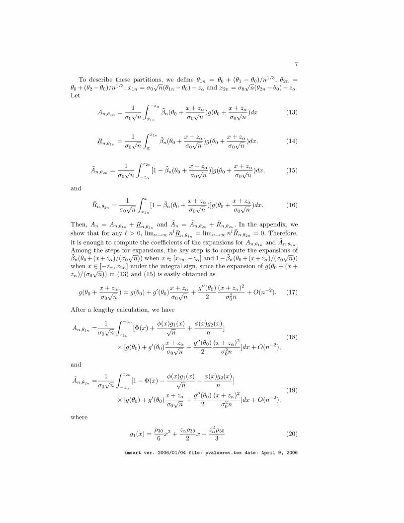
Fig 1. True and estimated values of δn as functions of α for the standard normal prior andthe Cauchy prior.

3.1. Examples

Example 1: Let X1, · · · ,Xn be i.i.d. N(θ, 1). Since θ is a location parameter,there is no loss of generality in letting θ0 = 0. Thus consider testing H0 : θ ≤0 vs H1 : θ > 0. Clearly, we have µ(θ) = θ, σ(θ) = 1 and ρi(θ) = κi(θ) = 0 forall i ≥ 3.

The α (0 < α < 1) level UMP test rejects H0 if√

nX > zα. For a continuouslythree times differentiable prior g(θ) for θ, one can simply plug the values of µ0 =0, σ0 = 1, ρ30 = ρ40 = 0 into (23) and the coefficients of the expansion in (24)to get the coefficients a1 = g(0)[Φ(zα)−αzα], a2 = −g′(0)[α(z2

α −1)−zαφ(zα)],a3 = g′′(0)[(zα + 2)φ(zα) − α(z3

α + 3zα)]/6, a1 = g(0)[φ(zα) + φ(zα)], a2 =g′(0)[(1−α)(z2

α+1)+zαφ(zα)]/2, a3 = g′′(0)[(zα+2)φ(zα)+(1−α)(z3α+3zα)]/6.

Substituting a1, a2, a3, a1, a2 and a3 into (7), one derives the expansions of δn

and εn as given by (1) and (2) respectively.If the prior density function is in addition assumed to be symmetric, then λ =

1/2 and g′(0) = 0. In this case, the coefficients of the expansion of δn in (1) aregiven explicitly as follows: c1 = 2g(0)[φ(zα)−αzα], c2 = 4zα[g(0)]2[φ(zα)−αzα],c3 = 2φ(zα)4z2

α[g(0)]3 + g′′(0)(z2α +2)/6−αg′′(0)(z3

α +3zα)/3+8z3α[g(0)]3,

and the coefficients of the expansions of εn in (2) are as d1 = 2g(0)[(1−α)zα +φ(zα)], d2 = −4zα[g(0)]2[(1−α)zα+φ(zα)], d3 = 2φ(zα)4z2

α[g(0)]3+g′′(0)(z2α+

2)/6 + (1 − α)g′′(0)(z3α + 3zα)/3 + 8z3

α[g(0)]3.Two specific prior distributions for θ are now considered for numerical illus-

tration. In the first one we choose θ ∼ N(0, τ2) and in the second example we


10

0.0 0.1 0.2 0.3 0.4 0.50.

10.

20.

30.

40.

5

n=5

α

ε n


0.0 0.1 0.2 0.3 0.4 0.5

0.10

0.20

0.30

0.40

n=10

α

ε n


0.0 0.1 0.2 0.3 0.4 0.5

0.05

0.10

0.15

0.20

0.25

0.30

n=10

α

ε n


0.0 0.1 0.2 0.3 0.4 0.5

0.05

0.10

0.15

0.20

n=20

α

ε n


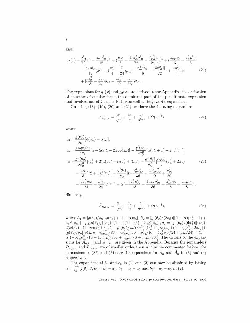
Fig 2. True and estimated values of εn as functions of α for the standard normal prior andthe Cauchy prior.

choose θ/τ ∼ tm, where τ is a scale parameter. Clearly g(3)(θ) is continuous inθ in both cases.

If g(θ) is the density of θ when θ ∼ N(0, τ2), then λ = 1/2, g(0) = 1/[√

2πτ ],g′(0) = 0 and g′′(0) = −1/[

√2πτ3].

We calculated the numerical values of c1, c2, c3, d1, d2 and d3 as functionsof α when θ ∼ N(0, 1). We note that c1 is a monotone increasing function andd1 is also a monotone decreasing function of α. However, c2, d2 and c3, d3 arenot monotone and in fact, d2 is decreasing when α is close to 1 (not shown), c3

also takes negative values and d3 takes positive values for larger values of α.If g(θ) is the density of θ when θ/τ ∼ tm, then λ = 1/2, g′(0) = 0, g(0) =

Γ(m+12 )/[τ

√mπΓ(m

2 )] and g′′(0) = −Γ(m+32 )/[τ

√mπΓ(m+2

2 )]. Putting thosevalues into the corresponding expressions, we get the coefficients c1, c2, c3 andd1, d2, d3 of the expansions of δn and εn. When m = 1, the results are exactlyfor the Cauchy prior for θ.

Numerical results very similar to the normal prior are seen for the Cauchycase. From Figure 1, we see that for each of the normal and the Cauchy prior,only about 1% of those null hypotheses a frequentist rejects with a p-value of lessthan 5% are true. Indeed quite typically, δn < α for even very small values ofn. This is discussed in greater detail in Section 4.5. This finding seems to us tobe quite interesting.

The true values of δn and εn are computed by taking an average of the lowerand the upper Riemann sums in An, An, Bn and Bn with the exact formulae forthe standard normal pdf. The accuracy of the expansion for δn is remarkable, as


11

0.0 0.1 0.2 0.3 0.4 0.5

0.00

0.05

0.10

0.15

0.20

0.25

0.30

n=5

α

δ nTrue(Gamma)Estimated(Gamma)True(F)Estimated(F)

0.0 0.1 0.2 0.3 0.4 0.5

0.00

0.05

0.10

0.15

0.20

n=10

α

δ n

True(Gamma)Estimated(Gamma)True(F)Estimated(F)

0.0 0.1 0.2 0.3 0.4 0.5

0.00

0.04

0.08

0.12

n=20

α

δ n


0.0 0.1 0.2 0.3 0.4 0.5

0.00

0.02

0.04

0.06

0.08

n=40

α

δ n


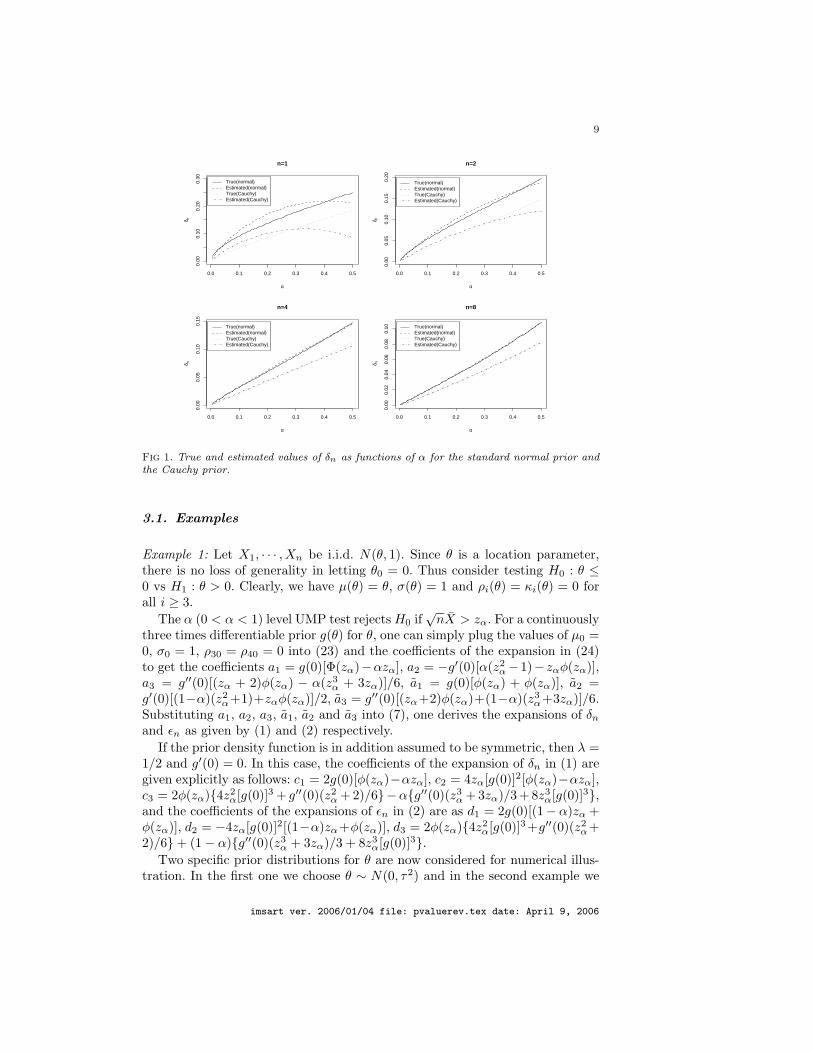
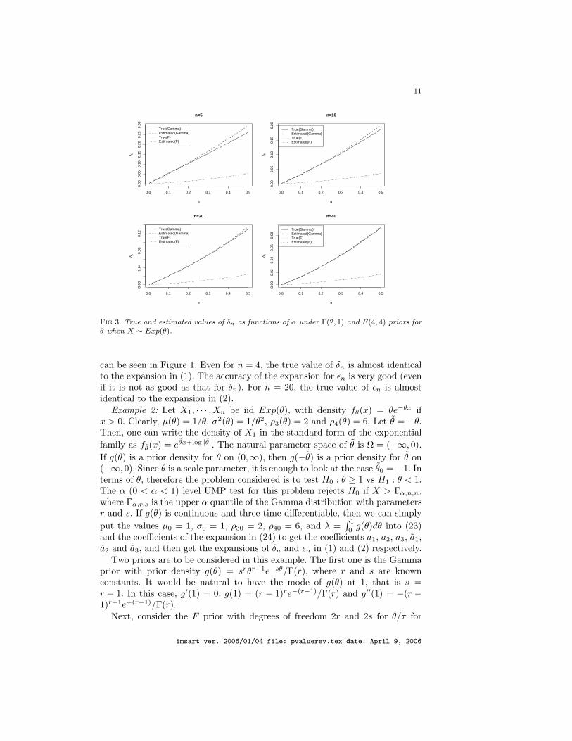
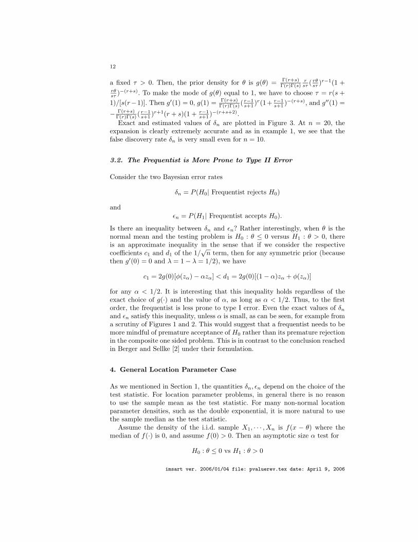
Fig 3. True and estimated values of δn as functions of α under Γ(2, 1) and F (4, 4) priors forθ when X ∼ Exp(θ).

can be seen in Figure 1. Even for n = 4, the true value of δn is almost identicalto the expansion in (1). The accuracy of the expansion for εn is very good (evenif it is not as good as that for δn). For n = 20, the true value of εn is almostidentical to the expansion in (2).

Example 2: Let X1, · · · ,Xn be iid Exp(θ), with density fθ(x) = θe−θx ifx > 0. Clearly, µ(θ) = 1/θ, σ2(θ) = 1/θ2, ρ3(θ) = 2 and ρ4(θ) = 6. Let θ = −θ.Then, one can write the density of X1 in the standard form of the exponentialfamily as fθ(x) = eθx+log |θ|. The natural parameter space of θ is Ω = (−∞, 0).If g(θ) is a prior density for θ on (0,∞), then g(−θ) is a prior density for θ on(−∞, 0). Since θ is a scale parameter, it is enough to look at the case θ0 = −1. Interms of θ, therefore the problem considered is to test H0 : θ ≥ 1 vs H1 : θ < 1.The α (0 < α < 1) level UMP test for this problem rejects H0 if X > Γα,n,n,where Γα,r,s is the upper α quantile of the Gamma distribution with parametersr and s. If g(θ) is continuous and three time differentiable, then we can simplyput the values µ0 = 1, σ0 = 1, ρ30 = 2, ρ40 = 6, and λ =

∫ 1

0g(θ)dθ into (23)

and the coefficients of the expansion in (24) to get the coefficients a1, a2, a3, a1,a2 and a3, and then get the expansions of δn and εn in (1) and (2) respectively.

Two priors are to be considered in this example. The first one is the Gammaprior with prior density g(θ) = srθr−1e−sθ/Γ(r), where r and s are knownconstants. It would be natural to have the mode of g(θ) at 1, that is s =r − 1. In this case, g′(1) = 0, g(1) = (r − 1)re−(r−1)/Γ(r) and g′′(1) = −(r −1)r+1e−(r−1)/Γ(r).

Next, consider the F prior with degrees of freedom 2r and 2s for θ/τ for


12

a fixed τ > 0. Then, the prior density for θ is g(θ) = Γ(r+s)Γ(r)Γ(s)

rsτ ( rθ

sτ )r−1(1 +rθsτ )−(r+s). To make the mode of g(θ) equal to 1, we have to choose τ = r(s +1)/[s(r−1)]. Then g′(1) = 0, g(1) = Γ(r+s)

Γ(r)Γ(s) (r−1s+1 )r(1+ r−1

s+1 )−(r+s), and g′′(1) =

− Γ(r+s)Γ(r)Γ(s) (

r−1s+1 )r+1(r + s)(1 + r−1

s+1 )−(r+s+2).Exact and estimated values of δn are plotted in Figure 3. At n = 20, the

expansion is clearly extremely accurate and as in example 1, we see that thefalse discovery rate δn is very small even for n = 10.

3.2. The Frequentist is More Prone to Type II Error

Consider the two Bayesian error rates

δn = P (H0| Frequentist rejects H0)

andεn = P (H1| Frequentist accepts H0).

Is there an inequality between δn and εn? Rather interestingly, when θ is thenormal mean and the testing problem is H0 : θ ≤ 0 versus H1 : θ > 0, thereis an approximate inequality in the sense that if we consider the respectivecoefficients c1 and d1 of the 1/

√n term, then for any symmetric prior (because

then g′(0) = 0 and λ = 1 − λ = 1/2), we have

c1 = 2g(0)[φ(zα) − αzα] < d1 = 2g(0)[(1 − α)zα + φ(zα)]

for any α < 1/2. It is interesting that this inequality holds regardless of theexact choice of g(·) and the value of α, as long as α < 1/2. Thus, to the firstorder, the frequentist is less prone to type I error. Even the exact values of δn

and εn satisfy this inequality, unless α is small, as can be seen, for example froma scrutiny of Figures 1 and 2. This would suggest that a frequentist needs to bemore mindful of premature acceptance of H0 rather than its premature rejectionin the composite one sided problem. This is in contrast to the conclusion reachedin Berger and Sellke [2] under their formulation.

4. General Location Parameter Case

As we mentioned in Section 1, the quantities δn, εn depend on the choice of thetest statistic. For location parameter problems, in general there is no reasonto use the sample mean as the test statistic. For many non-normal locationparameter densities, such as the double exponential, it is more natural to usethe sample median as the test statistic.

Assume the density of the i.i.d. sample X1, · · · ,Xn is f(x − θ) where themedian of f(·) is 0, and assume f(0) > 0. Then an asymptotic size α test for

H0 : θ ≤ 0 vs H1 : θ > 0


13

rejects H0 if√

nTn > zα/[2f(0)], where Tn = X([ n2 ]+1) is the sample median

[8, pp 89], since√

n(Tn − θ) L⇒ N(0, 1/[4f2(0)]). We will derive the coefficientsc1, c2, c3 in (1) and d1, d2, d3 in (2) given the prior density g(θ) for θ. We as-sume again that g(θ) is three times differentiable with a bounded absolute thirdderivative.

4.1. Expansion of Type I Error and Type II Error

To obtain the coefficients of the expansions of δn in (1) and εn in (2), we haveto expand the An and An given by (3) and (4). Of these,

An = P (θ ≤ 0,√

nTn >zα

2f(0)) =

1√n

∫ 0

−∞1 − Fn[zα − 2xf(0)]g(

x√n

)dx (25)

where Fn is the CDF of 2f(0)√

n(Tn−θ) if the true median is θ. Reiss [16] givesthe expansion of Fn as

Fn(t) = Φ(t) +φ(t)√

nR1(t) +

φ(t)n

R2(t) + rt,n, (26)

where, with x denoting the fractional part of a real x, R1(t) = f11t2 + f12,

f11 = f ′(0)/[4f2(0)], f12 = −(1 − 2n2 ), and R2(t) = f21t

5 + f22t3 + f23t,

where f21 = −[f ′(0)/f2(0)]2/32, f22 = 1/4 + (1/2 − n2 )[f ′(0)/(2f2(0))] +

f ′′(0)/[24f3(0)], f23 = 1/4− (1−2n2 )2/2. The error term r1,t,n can be written

as rt,n = φ(t)R3(t)/n3/2 + O(n−2), where R3(t) is a polynomial.By letting y = 2xf(0) − zα in (25), we have

An =1

2f(0)√

n

∫ −zα

−∞Φ(y) − φ(y)√

nR1(−y) − φ(y)

nR2(−y) − r−y,n

× [g(0) + g′(0)y + zα

2f(0)√

n+

g′′(0)2

(y + zα)2

4f2(0)n+

(y + zα)3

48f3(0)n3/2g(3)(y∗)]dy,

(27)

where y∗ is between 0 and (y + zα)/[2f(0)√

n].Hence, assuming supθ |g(3)(θ)| < ∞, on exact integration of each product of

functions in (27) and on collapsing the terms, we get

An =a1√n

+a2

n+

a3

n3/2+ O(n−2), (28)

where

a1 =g(0)2f(0)

[φ(zα) − αzα], (29)

a2 =g′(0)

8f2(0)[zαφ(zα) − α(z2

α + 1)] − g(0)2f(0)

f11[zαφ(zα) + α] + f12α (30)


14

and

a3 =g′′(0)

48f3(0)[(z2

α + 2)φ(zα) − α(z3α + 3zα)]

− g′(0)4f2(0)

f11[αzα − 2φ(zα)] + f12[αzα − φ(zα)]

− g(0)2f(0)

f21[(z4α + 4z2

α + 8)φ(zα)] + f22[(z2α + 2)φ(zα)] + f23φ(zα).

(31)

We claim the error term in (28) is O(n−2). To prove this, we need to look at itsexact form, namely,

−O(n−2)2f(0)

∫ −zα

−∞φ(y)R3(−y)g(θ0 +

y + zα

2f(0)√

n)dy + O(n−2)

∫ 0

−∞g(θ0 + y)dy.

Since g(θ) is an absolutely uniformly bounded, the first term above is boundedby O(n−2). The second term is O(n−2) obviously. This shows that the errorterm in (28) is O(n−2).

As regards An given by (4), one can similarly obtain

An =P (θ > 0,√

Tn ≤ zα

2f(0)) =

1√n

∫ ∞

0

Fn[zα − 2f(0)x]g(x√n

)dx

=a1√n

+a2

n+

a3

n32

+ O(n−2),(32)

where y∗ is between 0 and (zα − y)/[2f(0)√

n], a1 = [g(0)/(2f(0))][(1 − α)zα +φ(zα)], a2 = [g′(0)/(8f2(0))][(1−α)(z2

α +1)+zαφ(zα)]+[g(0)/(2f(0))]f11[(1−α)− zαφ(zα)]+f12(1−α), a3 = [g′′(0)/(48f3(0))][(z2

α +2)φ(zα)+(1−α)(z3α +

3zα)] + [g′(0)/(4f2(0))]f11[(1 − α)zα + 2φ(zα)] + f12[(1 − α)zα + φ(zα)] −[g(0)/(2f(0))]f21[(z4

α + 4z2α + 8)φ(zα)] + f22[(z2

α + 2)φ(zα)] + f23φ(zα). Theerror term in (32) is still O(n−2) and this proof is omitted.

Therefore, we have the the expansions of Bn given by (5) Bn = λ− b1/√

n−b2/n − b3/n3/2 + O(n−2) where λ =

∫∞0

g(θ)dθ as before, b1 = a1 − a1 =zαg(0)/[2f(0)], b2 = a2 − a2 = g′(0)(z2

α + 1)/[8f2(0)] + g(0)(f11 + f12)/[2f(0)],b3 = a3 − a3 = g′′(0)(z3

α + 3zα)/[48f3(0)] + zαg′(0)(f11 + f12)/[4f2(0)]. Substi-tuting a1, a2, a3, a1, a2, a3, b1, b2 and b3 into (7), we get the expansions of δn

and εn for the general location parameter case given by (1) and (2).

4.2. Testing with Mean vs. Testing with Median

Suppose X1, . . . , Xn are i.i.d. observations from a N(θ, 1) density and the statis-tician tests H0 : θ ≤ 0 vs. H1 : θ > 0 by using either the sample mean X orthe median Tn. It is natural to ask choice of which statistic makes him morevulnerable to false discoveries. We can look at both false discovery rates δn andεn to make this comparison, but we will do so only for the type I error rate δn

here.


15

0.0 0.1 0.2 0.3 0.4 0.5

0.00

0.05

0.10

0.15

n=10

α

δ n

TrueEstimated

0.0 0.1 0.2 0.3 0.4 0.5

0.00

0.02

0.04

0.06

0.08

0.10

n=20

α

δ n

TrueEstimated

0.0 0.1 0.2 0.3 0.4 0.5

0.00

0.02

0.04

0.06

0.08

n=30

α

δ n

TrueEstimated

0.0 0.1 0.2 0.3 0.4 0.5

0.00

0.02

0.04

0.06

n=40

α

δ n

TrueEstimated

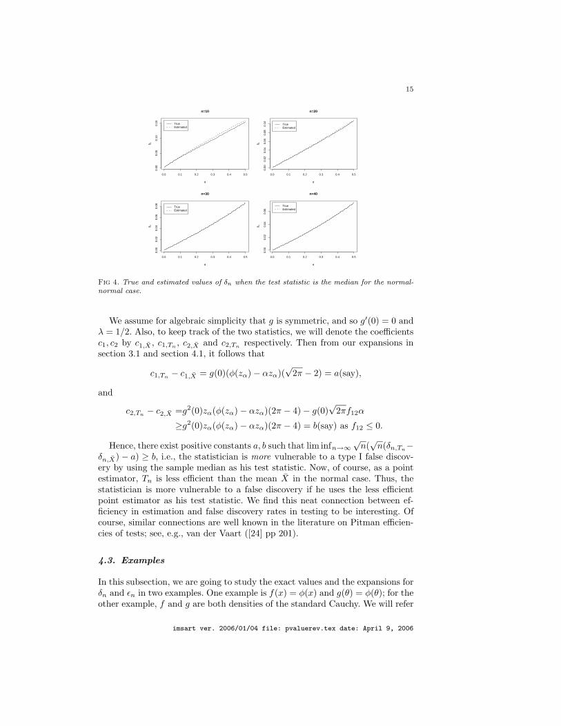
Fig 4. True and estimated values of δn when the test statistic is the median for the normal-normal case.

We assume for algebraic simplicity that g is symmetric, and so g′(0) = 0 andλ = 1/2. Also, to keep track of the two statistics, we will denote the coefficientsc1, c2 by c1,X , c1,Tn

, c2,X and c2,Tnrespectively. Then from our expansions in

section 3.1 and section 4.1, it follows that

c1,Tn− c1,X = g(0)(φ(zα) − αzα)(

√2π − 2) = a(say),

and

c2,Tn− c2,X =g2(0)zα(φ(zα) − αzα)(2π − 4) − g(0)

√2πf12α

≥g2(0)zα(φ(zα) − αzα)(2π − 4) = b(say) as f12 ≤ 0.

Hence, there exist positive constants a, b such that lim infn→∞√

n(√

n(δn,Tn−

δn,X) − a) ≥ b, i.e., the statistician is more vulnerable to a type I false discov-ery by using the sample median as his test statistic. Now, of course, as a pointestimator, Tn is less efficient than the mean X in the normal case. Thus, thestatistician is more vulnerable to a false discovery if he uses the less efficientpoint estimator as his test statistic. We find this neat connection between ef-ficiency in estimation and false discovery rates in testing to be interesting. Ofcourse, similar connections are well known in the literature on Pitman efficien-cies of tests; see, e.g., van der Vaart ([24] pp 201).

4.3. Examples

In this subsection, we are going to study the exact values and the expansions forδn and εn in two examples. One example is f(x) = φ(x) and g(θ) = φ(θ); for theother example, f and g are both densities of the standard Cauchy. We will refer


16

0.0 0.1 0.2 0.3 0.4 0.5

0.00

0.05

0.10

0.15

n=10

α

δ n

TrueEstimated

0.0 0.1 0.2 0.3 0.4 0.5

0.00

0.02

0.04

0.06

0.08

0.10

n=20

α

δ n

TrueEstimated

0.0 0.1 0.2 0.3 0.4 0.5

0.00

0.02

0.04

0.06

0.08

n=30

α

δ n

TrueEstimated

0.0 0.1 0.2 0.3 0.4 0.5

0.00

0.02

0.04

0.06

n=40

α

δ n

TrueEstimated

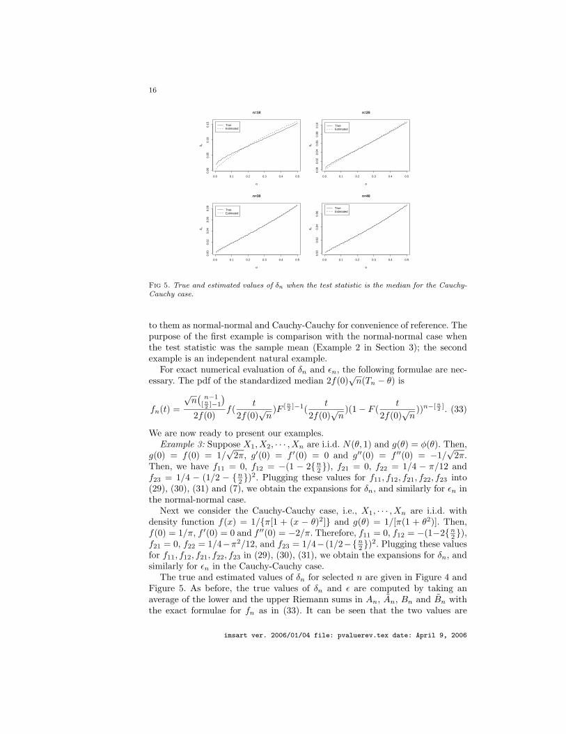
Fig 5. True and estimated values of δn when the test statistic is the median for the Cauchy-Cauchy case.

to them as normal-normal and Cauchy-Cauchy for convenience of reference. Thepurpose of the first example is comparison with the normal-normal case whenthe test statistic was the sample mean (Example 2 in Section 3); the secondexample is an independent natural example.

For exact numerical evaluation of δn and εn, the following formulae are nec-essary. The pdf of the standardized median 2f(0)

√n(Tn − θ) is

fn(t) =

√n(

n−1[ n2 ]−1

)2f(0)

f(t

2f(0)√

n)F [ n

2 ]−1(t

2f(0)√

n)(1 − F (

t

2f(0)√

n))n−[ n

2 ]. (33)

We are now ready to present our examples.Example 3: Suppose X1,X2, · · · ,Xn are i.i.d. N(θ, 1) and g(θ) = φ(θ). Then,

g(0) = f(0) = 1/√

2π, g′(0) = f ′(0) = 0 and g′′(0) = f ′′(0) = −1/√

2π.Then, we have f11 = 0, f12 = −(1 − 2n

2 ), f21 = 0, f22 = 1/4 − π/12 andf23 = 1/4 − (1/2 − n

2 )2. Plugging these values for f11, f12, f21, f22, f23 into(29), (30), (31) and (7), we obtain the expansions for δn, and similarly for εn inthe normal-normal case.

Next we consider the Cauchy-Cauchy case, i.e., X1, · · · ,Xn are i.i.d. withdensity function f(x) = 1/π[1 + (x − θ)2] and g(θ) = 1/[π(1 + θ2)]. Then,f(0) = 1/π, f ′(0) = 0 and f ′′(0) = −2/π. Therefore, f11 = 0, f12 = −(1−2n

2 ),f21 = 0, f22 = 1/4−π2/12, and f23 = 1/4− (1/2−n

2 )2. Plugging these valuesfor f11, f12, f21, f22, f23 in (29), (30), (31), we obtain the expansions for δn, andsimilarly for εn in the Cauchy-Cauchy case.

The true and estimated values of δn for selected n are given in Figure 4 andFigure 5. As before, the true values of δn and ε are computed by taking anaverage of the lower and the upper Riemann sums in An, An, Bn and Bn withthe exact formulae for fn as in (33). It can be seen that the two values are


17

almost identical when n = 30. By comparison with Figure 1, we see that theexpansion for median is not as precise as the expansion for the sample mean.

The most important thing we learn is how small δn is for very moderatevalues of n. For example, in Figure 4, δn is only about 0.01 if α = 0.05, whenn = 20. Again we see that even though we have changed the test statistic to themedian, the frequentist’s false discovery rate is very small and, in particular,smaller than α. More about this is said in Sections 4.4 and 4.5.

4.4. Spiky Priors and False Discovery Rates

We commented in Section 4.1 that if the prior density g(θ0) is large, it increasesthe leading term in the expansion for δn (and also εn) and so it can be expectedthat spiky priors cause higher false discovery rates. In this section, we addressthe effect of spiky and flat priors a little more formally.

Consider the general testing problem H0 : θ ≤ θ0 vs H1 : θ > θ0, where thenatural parameter space Ω = (θ, θ).

Suppose the α (0 < α < 1) level test rejects H0 if Tn ∈ C, where Tn is thetest statistic. Let Pn(θ) = Pθ(Tn ∈ C). Let g(θ) be any fixed density functionfor θ and let gτ (θ) = g(θ/τ)/τ , τ > 0. Then gτ (θ) is spiky at 0 for small τ andgτ (θ) is flat for large τ . When θ0 = 0, under the prior gτ (θ),

δn(τ) = P (θ ≤ 0|Tn ∈ C) =

∫ 0

θ/τPn(τy)g(y)dy∫ θ/τ

θ/τPn(τy)g(y)dy

, (34)

and

εn(τ) = P (θ > 0|Tn 6∈ C) =

∫ 0

θ/τ[1 − Pn(τy)]g(y)dy∫ θ/τ

θ/τ[1 − Pn(τy)]g(y)dy

. (35)

Let as before λ =∫ 0

−∞ g(θ)dθ, the numerator and denominator of (34) be de-noted by An(τ) and Bn(τ) and the numerator and denominator of (35) bedenoted by An(τ) and Bn(τ). Then, we have the following results.

Proposition 1 If P−n (θ0) = limθ→θ0− Pn(θ) and P+

n (θ0) = limθ→θ0+ Pn(θ)both exist and are positive, then

limτ→0

δn(τ) =λP−

n (0)λP−

n (0) + (1 − λ)P+n (0)

(36)

and

limτ→0

εn(τ) =(1 − λ)[1 − P+

n (0)]λ[1 − P−

n (0)] + (1 − λ)[1 − P+n (0)]

. (37)

Proof: Because 0 ≤ Pn(τy) ≤ 1 for all y, by simply applying the LebesgueDominated Convergence Theorem, limτ→0 An(τ) = λP−

n (0), limτ→0 Bn(τ) =


18

λP−n (0)+(1−λ)P+

n (0), limτ→0 An(τ) = (1−λ)[1−P+n (0)] and limτ→0 Bn(τ) =

λ[1 − P−n (0)] + (1 − λ)[1 − P+

n (0)]. Substituting in (34) and (35), we get (36)and (37).

Corollary 1 If 0 < λ < 1, limτ→∞ Pn(τy) = 0 for all y < 0, limτ→∞ Pn(τy) =1 for all y > 0, then limτ→∞ δn(τ) = limτ→∞ εn(τ) = 0.

Proof: Immediate from (36) and (37).

It can be seen that P−n (0) = P+

n (0) in most testing problems when the teststatistic Tn has a continuous power function. It is true for all the problems wediscussed in Sections 3 and 4. If moreover g(θ) > 0 for all θ, then 0 < λ < 1. Asa consequence, limτ→0 δn(τ) = λ, limτ→0 εn(τ) = 1 − λ, and limτ→∞ δn(τ) =limτ→∞ εn(τ) = 0. If θ is a location parameter, θ0 = 0 and g(θ) is symmetricabout 0, then limτ→0 δn(τ) = limτ→0 εn(τ) = 1/2.

In other words, the false discovery rates are very small for any n for flatpriors and roughly 50% for any n for very spiky symmetric priors. This is aqualitatively informative observation.

4.5. Pre-experimental Promise and Post-experimental Honesty

We noticed in our example in Section 4.4 that for quite small values of n, thepost-experimental error rate δn was smaller than the pre-experimental assur-ance, namely α. For any given prior g, this is true for all large n; but clearlywe cannot achieve this uniformly over all g, or even large classes of g. In orderto remain honest, it seems reasonable to demand of a frequentist that δn besmaller than α. The question is, typically for what sample sizes the frequentistcan assert his honesty.

Let us then consider the prior gτ (θ) = g(θ/τ)/τ with fixed g, and considerthe minimum value of the sample size n, denoted by nα(τ), such that δn ≤ α.It can be seen from (36) that nα(τ) goes to ∞ as τ goes to 0. This of coursewas anticipated. What happens when τ varies from small to large values?

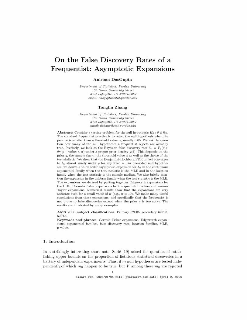
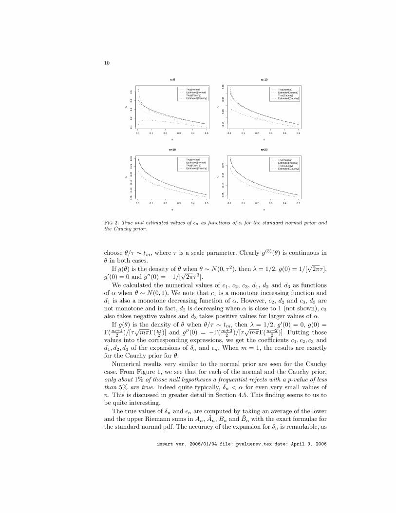
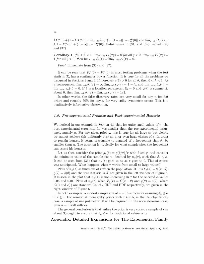
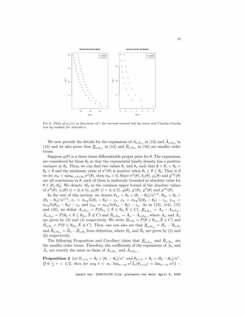
Plots of nα(τ) as functions of τ when the population CDF is Fθ(x) = Φ(x−θ),g(θ) = φ(θ) and the test statistic is X are given in the left window of Figure 6.It is seen in the plot that nα(τ) is non-increasing in τ for the selected α-values0.05 and 0.01. Plots of nα(τ) when Fθ(x) = C(x − θ) and g(θ) = c(θ), whereC(·) and c(·) are standard Cauchy CDF and PDF respectively, are given in theright window of Figure 6.

In both examples, a modest sample size of n = 15 suffices for ensuring δn ≤ αif τ ≥ 1. For somewhat more spiky priors with τ ≈ 0.5, in the Cauchy-Cauchycase, a sample of size just below 30 will be required. In the normal-normal case,even n = 8 still suffices.

The general conclusion is that unless the prior is very spiky, a sample of sizeabout 30 ought to ensure that δn ≤ α for traditional values of α.

Appendix: Detailed Expansions for The Exponential Family


19

−1.0 −0.5 0.0

510

1520

Normal−Normal by Mean

log(τ)

n α(τ

)

o

o

o

o

o

o

o

o

o

o

o

o

o

o

o

o

o

o

o

o

x

x

x

x

x

x

x

x

x

x

x

x

x

x

x

x

x

x

x

x α=0.05α=0.01

ox

−1 0 1 2 3 4 5

510

15

Cauchy−Cauchy by Median

log(τ)n α

(τ)

o

o

o

o

o

o

o

o

o

o

x

x

x

x

x

x

x

x

x

x α=0.05α=0.01

ox

Fig 6. Plots of nα(τ) as functions of τ for normal-normal test by mean and Cauchy-Cauchytest by median for selected α.

We now provide the details for the expansions of An,θ1nin (13) and An,θ2n

in(15) and we also prove that Rn,θ1n

in (14) and Rn,θ2nin (16) are smaller order

terms.Suppose g(θ) is a three times differentiable proper prior for θ. The expansions

are considered for those θ0 so that the exponential family density has a positivevariance at θ0. Then, we can find two values θ1 and θ2 such that θ < θ1 < θ0 <θ2 < θ and the minimum value of σ2(θ) is positive when θ1 ≤ θ ≤ θ2. That is ifwe let m0 = minθ1<θ<θ2 σ2(θ), then m0 > 0. Since σ2(θ), ki(θ), ρi(θ) and g(3)(θ)are all continuous in θ, each of them is uniformly bounded in absolute value forθ ∈ [θ1, θ2]. We denote M0 as the common upper bound of the absolute valuesof σ2(θ), κi(θ) (i = 3, 4, 5), ρi(θ) (i = 3, 4, 5), g(θ), g′(θ), g′′(θ) and g(3)(θ).

In the rest of this section, we denote θ1n = θ0 + (θ1 − θ0)/n1/3, θ2n = θ0 +(θ2 − θ0)/n1/3, x1 = σ0

√n(θ1 − θ0) − zα, x2 = σ0

√n(θ2 − θ0) − zα, x1n =

σ0√

n(θ1n − θ0) − zα and x2n = σ0√

n(θ1n − θ0) − zα. As in (13), (14), (15)and (16), we define An,θ1n

= P (θ1n ≤ θ ≤ θ0, X ∈ C), Rn,θ1n= An − An,θ1n

,An,θ2n

= P (θ0 < θ ≤ θ2n, X 6∈ C) and Rn,θ2n= An − An,θ2n

, where An and An

are given by (3) and (4) respectively. We write Bn,θ1 = P (θ ≥ θ1n, X ∈ C) andBn,θ2 = P (θ ≤ θ2n, X 6∈ C). Then, one can also see that Rn,θ1n

= Bn − Bn,θ1

and Rn,θ2n= Bn− Bn,θ2 from definition, where Bn and Bn are given by (5) and

(6) respectively.The following Proposition and Corollary claim that Rn,θ1n

and Rn,θ2nare

the smaller order terms. Therefore, the coefficients of the expansions of An andAn are exactly the same as those of An,θ1n

and An,θ2n.

Proposition 2 Let θ1,τ,n = θ0 + (θ1 − θ0)/nτ and θ2,τ,n = θ0 + (θ2 − θ0)/nτ .If 0 ≤ τ < 1/2, then for any ` < ∞, limn→∞ nlβn(θ1,τ,n) = limn→∞ nl[1 −


20

βn(θ2,τ,n)] = 0.

Proof: A proof of this can be obtained by simply using Markov’s inequality.We omit it. ♦Corollary 2 For any l > 0, limn→∞ nlRn,θ1n

= limn→∞ nlRn,θ2n= 0.

Proof: Since βn(θ) is nondecreasing in θ, we have

nlRn,θ1n= nl

∫ θ1n

θ

βn(θ)g(θ)dθ ≤ nlβn(θ1,1/3,n)∫ θ1n

θ

g(θ)dθ ≤ nlβn(θ1,1/3,n)

and similarly nlRn,θ2n≤ nl[1− βn(θ2,1/3,n)]. The conclusion is drawn by taking

τ = 1/3 in Proposition (2). ♦In the rest of this section, we will only derive the expansion of An,θ1n

in detailsince the expansion of An,θ2n

is obtained exactly similarly.Using the transformation x = σ0

√n(θ− θ0)− zα in the following integral, we

have

An,θ1n=

1σ0

√n

∫ −zα

x1n

βn(θ0 +x + zα

σ0√

n)g(θ0 +

x + zα

σ0√

n)dx. (38)

Note that

βn(θ0 +x + zα

σ0√

n) = Pθ0+

x+zασ0

√n

(√

nX − µ(θ0 + x+zα

σ0√

n)

σ(θ0 + x+zα

σ0√

n)

≥ kθ0,x,n

), (39)

where

kθ0,x,n =

[√

nµ0 − µ(θ0 + x+zα

σ0√

n)

σ0+ kθ0,n

]σ0

σ(θ0 + x+zα

σ0√

n). (40)

We obtain the coefficients of the expansions of An,θ1nin the following steps:

1. The expansion of g(θ0 + x+zα

σ0√

n) for any fixed x ∈ [x1n,−zα] is obtained by

using Taylor expansions.2. The expansion of kθ0,x,n for any fixed x ∈ [x1n,−zα] is obtained by jointly

considering the Cornish-Fisher expansion of kθ0,n, the Taylor expansion of√n[µ0 − µ(θ0 + x+zα

σ0√

n)]/σ0 and the Taylor expansion of σ0/σ(θ0 + x+zα

σ0√

n).

3. Write the CDF of X in the form of Pθ[√

n X−µ(θ)σ(θ) ≤ u]. Formally substitute

θ = θ0 + x+zα

σ0√

nand u = kθ0,x,n in the Edgeworth expansion of the CDF

of X. An expansion of βn(θ0 + x+zα

σ0√

n) is obtained by combining it with

Taylor expansions for a number of relevant functions (see (47)).4. The expansion of An,θ1n

is obtained by considering the product of theexpansions of g(θ0 + x+zα

σ0√

n) and βn(θ0 + x+zα

σ0√

n) under the integral sign.

5. Finally prove that all the error terms in Steps 1, 2, 3 and 4 are smallerorder terms.


21

We give the expansions in steps 1, 2, 3 and 4 in detail. For the error termstudy in step 5, we omit the details due to the considerably tedious algebra.

Step 1: The expansion of g(θ0 + x+zα√n

) is easily obtained by using a Taylorexpansion:

g(θ0 +x + zα

σ0√

n) = g(θ0) + g′(θ0)

x + zα

σ0√

n+

g′′(θ0)2

(x + zα)2

σ20n

+ rg,x,n. (41)

where rg,x,n is the error term.Step 2: The Cornish-Fisher expansion of kθ0,n [1, pp 117] is given by

kθ0,n = zα +(z2

α − 1)ρ30

6√

n+

1n

[(z3

α − 3zα)ρ40

24− (2z3

α − 5zα)ρ230

36

]+ r1,n, (42)

where r1,n is the error term.The Taylor expansion of the first term inside the bracket of (40) is

−(x + zα) − ρ30(x + zα)2

2√

n− ρ40(x + zα)3

6n+ r2,x,n (43)

and the Taylor expansion of the term outside of the bracket of (40) is

1 − ρ30(x + zα)2√

n+

1n

(3ρ2

30

8− ρ40

4

)(x + zα)2 + r3,x,n, (44)

where r2,x,n and r3,x,n are error terms.Plugging (42), (43) and (44) into (40), we get the expansion of kθ0,x,n below:

kθ0,x,n = −x +1√n

f1(x) +1n

f2(x) + r4,x,n, (45)

where r4,x,n is the error term, f1(x) = f11x + f10 and f2(x) = f23x3 + f22x

2 +f21x + f20, and the coefficients for f1(x) and f2(x) are f10 = −(2z2

α + 1)ρ30/6,f11 = −zαρ30/2, f20 = (z3

α + 2zα)ρ230/9 − (z3

α + zα)ρ40/8, f21 = (7z2α/24 +

1/12)ρ230 − z2

αρ40/4, f22 = 0, f23 = ρ40/12 − ρ230/8.

Step 3: The Edgeworth expansion of the CDF of X is (Barndorff-Nielsenand Cox [1, pp 91] and Hall [12, pp 45]) given below:

Pθ0+x+zασ0

√n

√

nX − µ(θ0 + x+zα

σ0√

n)√

σ(θ0 + x+zα

σ0√

n)

≤ u

=Φ(u) − φ(u)√n

(u2 − 1)6

ρ3(θ0 +x + zα

σ0√

n) − φ(u)

n[(u3 − 3u)

24

× ρ4(θ0 +x + zα

σ0√

n) +

(u5 − 10u3 + 15u)72

ρ23(θ0 +

x + zα

σ0√

n)] + r5,n,

(46)


22

where r5,n is an error term. If we take µ = kθ0,x,n in (46), then the left side is1 − βn(θ0 + x+zα√

n) and so

β(θ0 +x + zα

σ0√

n) = Φ(−kθ0,x,n) +

φ(kθ0,x,n)√n

(k2θ0,x,n − 1)

6ρ3(θ0 +

x + zα

σ0√

n)

+φ(kθ0,x,n)

n[(k3

θ0,x,n − 3kθ0,x,n)24

ρ4(θ0 +x + zα

σ0√

n)

+(k5

θ0,x,n − 10k3θ0,x,n + 15kθ0,x,n)72

ρ23(θ0 +

x + zα

σ0√

n)] − r5,n.

(47)

Plug the Taylor expansion of ρ3(θ0 + x+zα

σ0√

n)

ρ3(θ0 +x + zα

σ0√

n) = ρ30 +

(x + zα)√n

(ρ40 − 3

2ρ230

)+ r6,x,n (48)

in (47), where r6,x,n is an error term, and then consider the Taylor expansionsof the three terms related to kθ0,x,n in (47) and also use the expansion (45). Onquite a bit of calculations, we obtain the following expansion:

βn(θ0 +x + zα

σ0√

n) = Φ(x) − φ(x)

[f1(x)√

n+

f2(x)n

]− xφ(x)

[f1(x)√

n

]2

+φ(x)(x2 − 1)

6√

n[ρ30 +

(x + zα)√n

(ρ40 − 32ρ230)] +

ρ30

6nφ(x)(x3 − 3x)f1(x)

+φ(x)

n[(x3 − 3x)

24ρ40 +

(x5 − 10x3 + 15x)72

ρ230] + r7,x,n

=Φ(x) +φ(x)√

ng1(x) +

φ(x)n

g2(x) + r7,x,n,

(49)

where r7,x,n is an error term, g1(x) = g12x2 + g11x + g10, g2(x) = g20 + g21x +

g22x2 + g23x

3 + g24x4 + g25x

5, and the coefficients of g1(x) and g2(x) are g12 =ρ30/6, g11 = zαρ30/2, g10 = z2

αρ30/3, g25 = ρ230/72, g24 = −zαρ2

30/12, g23 =ρ40/8 − 13z2

αρ230/72 − 7ρ2

30/24, g22 = zαρ40/6 − z3αρ2

30/6 − zαρ230/12, g21 =

(z2α/4− 7/24)ρ40 − z4

αρ230/18− 13z2

αρ230/72 + 4ρ2

30/9, g20 = (z3α/8− zα/24)ρ40 −

(z3α/9 − zα/36)ρ2

30.Step 4: The expansion of An,θ1n

is obtained by plugging the expansions ofβ(θ0 + x+zα

σ0√

n) and g(θ0 + x+zα

σ0√

n). On careful calculations,

An,θ1n=

a1√n

+a2

n+

a3

n3/2+ r8,n, (50)

where r8,n is an error term, a1 = (g(θ0)/σ0)[φ(zα) − αzα], a2 = ρ30g(θ0)[α +2αz2

α−2zαφ(zα)]/(6σ0)−g′(θ0)[α(z2α+1)−zαφ(zα)]/(2σ2

0), and a3 = [h11φ(zα)+αh12][(g′′(θ0)/(6σ3

0)]+[h21φ(zα)+αh22][g′(θ0)/σ20 ]+[h31φ(zα)+αh32][g(θ0)/σ0],

where h11 = z2α + 2, h12 = −(z3

α + 3zα), h21 = −(ρ30/3)(z2α + 1), h22 =


23

(ρ30/3)(z3α + 2zα), h31 = −z4

αρ230/36 + 4z2

αρ230/9 + ρ2

30/36− 5z2αρ40/24 + ρ40/24,

h32 = −5z3αρ2

30/18 − 11zαρ230/36 + z3

αρ40/8 + zαρ40/8. These a1, a2 and a3 arethe coefficients in the expansion of (23).

The computation of the coefficients of the expansions of An,θ1nis now com-

plete. The rest of the work is to prove that all the error terms are smaller orderterms. But first we give the results for the expansion of An,θ2n

. The details forthe expansions of An,θ2n

are omitted.Expansion of An,θ2n

: The expansion of An,θ2ncan be obtained similarly by

simply repeating all the steps for An,θ1n. The results are given below:

An,θ2n=

a1√n

+a2

n+

a3

n3/2+ r9,n, (51)

where r9,n is an error term, a1 = g(θ0)[φ(zα) + (1 − α)zα]/σ0, a2 = g′(θ0)[(1 −α)(z2

α +1)+zαφ(zα)]/(2σ20)−ρ30g(θ0)[(1−α)/6+(1−α)z2

α/3+zαφ(zα)/3]/σ0,and a3 = (g′′(θ0)/6σ3

0)[h11φ(zα) − (1 − α)h12] − (g′(θ0)/σ20)[−h21φ(zα) + (1 −

α)h22] − (g(θ0)/σ0)[−h31φ(zα) + (1 − α)h32], where h11, h12, h21, h22, h31 andh32 are the same as defined in Step 3. These a1, a2 and a3 are the coefficientsin the expansion of (24).

Remark: The coefficients of expansions of δn and εn are obtained by simplyusing formula (7) with a1, a2 and a3 in (23) and also the coefficient a1, a2 anda3 in (24) respectively.

Step 5: (Error term study in the expansions of An,θ1n). We only give the

main steps because the details are too long. Recall from equation (38) that therange of integration corresponding to An,θ1n

is x1n ≤ x ≤ −zα. In this case, wehave limn→∞ x1n = ∞ and limn→∞ x1n/

√n = −zα. This fact is used when we

prove the error term is still a smaller order term when we move it out of theintegral sign.

(I) In (41), since g(3)(θ) is uniformly bounded in absolute values, rg,x,n isabsolutely bounded by a constant times n−3/2(x + zα)2

(II) From Barndorff-Nielsen and Cox [1, pp 117], the error term r1,n in (42) isabsolutely uniformly bounded by a constant times n−3/2.

(III) In (43) and (44), since ρi(θ) and κi(θ) (i = 3, 4, 5) are uniformly boundedin absolute values, the error term r2,x,n is absolutely bounded by a con-stant times n−3/2(x+zα)4 and the error term r3,x,n is absolutely boundedby a constant times n−3/2(x + zα)3.

(IV) The exact form of the error term r4,x,n in (45) can be derived by consid-ering the higher order terms and their products in (42), (43) and (44)for the derivation of expression (45). The computation is complicatedbut straightforward. However, still, since ρi(θ) and κi(θ) (i = 3, 4, 5) areuniformly bounded in absolute values, r4,x,n is absolutely bounded byn−3/2P1(|x|), where P1(|x|) is a seventh degree polynomial and its coeffi-cients do not depend on n.

(V) Again, from Barndorff-Nielsen and Cox [1, pp 91], the error term r5,n in(46) is absolutely bounded by a constant times n−3/2.


24

(VI) The error term r6,x,n in (48) is absolutely bounded by a constant timesn−1(x + zα)2 since ρi(θ) and κi(θ) (i = 3, 4, 5) are uniformly bounded inabsolute values.

(VII) This is the critical step for the error term study since we need to provethat the error term is still a smaller order term when it is moved outof the integral in (50). We need to study the behaviors of Φ(−kθ0,x,n)and φ(kθ0,x,n) as n → ∞ for all x ∈ [x1n,−zα] uniformly (see (49) indetail). This also explains why we choose θ1n = θ0 + (θ1 − θ0)/n1/3 andx1n = σ0

√n(θ1n − θ0) − zα at the beginning of this section, since in this

case |kθ0,x,n + x| is uniformly bounded by |x|/2 + 1 for a sufficiently largen. Then for sufficiently large n, the error term |r7,x,n| in (49) is uniformlybounded by |r7,x,n| ≤ φ(x/2+1)P2(|x|) where P2(|x|) is a twelveth degreepolynomial of |x| and its coefficients do not depend on n.

(VIII) Finally, we can show that the error term r8,n in (50) in O(n−2). This istedious but straightforward. It is proven by considering each of the tenterms in r8,n separately.

Remark: We can similarly prove that the error term r9,n in (51) correspond-ing to An,θ2n

is O(n−2). Since the steps are very similar, we do not mentionthem.

Acknowledgment: It is a pleasure to thank Michael Woodroofe for thenumerous conversations we had with him on the foundational questions andthe technical aspects of this paper. This paper would have never been writtenwithout Michael’s association. We would also like to thank two anonymousreferees for their thoughtful remarks and Jiayang Sun for her editorial input.We thank Larry Brown for reading an earlier draft of the paper and for givingus important feedback and to Persi Diaconis for asking a question that helpedus in interpreting the results.

References

[1] Barndorff-Nielsen, O.E., and Cox, D.R. (1989). Asymptotic techniques foruse in statistics. Chapman and Hall, New York.

[2] Berger, J and Sellke, T. (1987). Testing a point null hypothesis: the irrecon-cilability of P values and evidence. J. Amer. Statist. Assoc., 82, 112-122.

[3] Benjamini, Y. and Hochberg, Y. (1995). Controlling the false discovery rate:a practical and powerful approach to multiple testing. J. R. Stat. Soc. Ser.B, 57, 289-300.

[4] Edwards, W., Lindman, H. and Savage, L. J. (1984). Bayesian statisticalinference for psychological research. Robustness of Bayesian analyses, 1-62,Stud. Bayesian Econometrics, 4, North-Holland, Amsterdam, 1984.

[5] Efron, B. (2003). Robbins, empirical Bayes and microarrays. Ann. Statist.,31, 366-378.

[6] Brown, L. (1986). Fundamentals of Statistical Exponential Families with Ap-plications in Statistical Decision Theory. Institute of Mathematical Statis-tics. Hayward, California.


25

[7] Casella, G. and Berger, R.L. (1987). Reconciling Bayesian and frequentistevidence in the one-sided testing problem. J. Amer. Statist. Assoc., 82, 106-111.

[8] Ferguson, T. (1996). A Course in Large Sample Theory. Chapman & Hall,New York.

[9] Finner, H. and Roters, M. (2001). On the false discovery rate and expectedtype I errors. Biom. J., 43, 985-1005.

[10] Genovese, C. and Wasserman, L. (2002). Operating characteristics and ex-tensions of the false discovery rate procedure. J. R. Stat. Soc. Ser. B, 64,499-517.

[11] Hall, P. and Sellinger, B. (1986). Statistical significance: balancing evidenceagainst doubt. Australian J. of Statist., 28, 354-370.

[12] Hall, P. (1992). The Bootstrap And Edgeworth Expansion. Springer-Verlag,New York.

[13] Lehmann, E.L. (1986). Hypothesis Testing. Wiley, New York.[14] Marden, J. (2000). Hypothesis testing: from p values to Bayes factors. J.

Amer. Statist. Assoc., 95, 1316-1320.[15] Petrov, V. V. (1995). Limit Theorems of Probability Theory: Sequences of

Independent Random Variables. Oxford University Press, Oxford, UK.[16] Reiss, R.D. (1976). Asymptotic expansion for sample quantiles, Ann. Prob.,

4, 249-258.[17] Schervish, M. (1996). P values: what they are and what they are not. Amer-

ican Statistician, 50, 203-206.[18] Sellke, T., Bayarri, M.J. and Berger, J. (2001). Calibration of p values for

testing precise null hypotheses. American Statistician, 55, 62-71.[19] Soric, B. (1989). Statistical “discoveries” and effect-size estimation. J.

Amer. Statist. Assoc., 84, 608-610.[20] Storey, J. D. (2002). A direct approach to false discovery rate. J. R. Stat.

Soc. Ser. B, 64, 479-498.[21] Storey, J. D. (2003). The positive false discovery rate: a Bayesian interpre-

tation and the p-value. Ann. Statist., 31, 2013-2035.[22] Storey, J. D. and Tibshirani, R. (2003). Statistical significance for

genomewide studies. Proc. Natl. Acad. Sci. USA 100, 16, 9440-9445 (elec-tronic).

[23] Storey, J. D., Taylor, J. E. and Siegmund, D. (2004). Strong control, con-servative point estimation and simultaneous conservative consistency of falsediscovery rates: a unified approach. J. R. Stat. Soc. Ser. B, 66, 187-205.

[24] van der Vaart, A.W. (1998). Asymptotic statistics, Cambridge UniversityPress, Cambridge, UK.


On the False Discovery Rates of a Frequentist: Asymptotic ...

Documents

Transcript of On the False Discovery Rates of a Frequentist: Asymptotic ...