Nilpotent groups, asymptotic cones and subfinsler geometry
36
NILPOTENT GROUPS, ASYMPTOTIC CONES AND SUBFINSLER GEOMETRY EMMANUEL BREUILLARD AND ENRICO LE DONNE Abstract. We give an estimate of the speed of convergence of Cayley graphs of general finitely generated nilpotent groups towards their asymptotic cone. This yields an error term in the asymp- totics for the volume of large balls, namely |B(n)| = cn d + O(n d-α ), where the exponent α> 0 in the error term depends only on the nilpotency class. Conjecturally this holds for α = 1. We relate this conjecture to other well-known conjectures in subRiemannian geometry and show that abnormal geodesics play an important role. We also study in some detail the geometry of the Heisenberg group (equipped with the Pansu metric) and show that our results are sharp for 2-step groups by giving an example for which the speed of convergence to the asymptotic cone is no faster than n - 1 2 . Contents 1. Introduction 1 2. SubFinsler metrics and dilations on nilpotent Lie groups 5 3. Approximation by horizontal paths and discretization of continuous geodesics 14 4. Proofs of the main results 17 5. Sharpness of the error terms for step-2 groups and the Burago-Margulis conjecture 22 6. Volume of Cayley spheres, regularity of subFinsler spheres and other open problems 31 References 35 1. Introduction Let Γ be a nilpotent group generated by a finite set of elements S. We will assume that 1 ∈ S and that S = S −1 . Following earlier results of Wolf [22], Bass [3], and Guivarc’h [12], Pansu [17] established in 1983 that the cardinality of the balls S n = S · ... · S of radius n for the word metric induced by S on the Cayley graph of G is asymptotic to c S n d , where c S > 0 is a positive constant depending on S and d is an integer independent of S and given by the Bass-Guivarc’h formula: (1.1) d = ∑ k>1 kd k , where d k is the rank of the Abelian group C k (Γ)/C k+1 (Γ), where C 1 (Γ) = Γ, C i+1 (Γ) = [Γ,C i (Γ)] for i > 1, is the central descending series of Γ. Date : December 7, 2012. 1991 Mathematics Subject Classification. 53C17,22E25. Key words and phrases. subRiemannian geometry, polynomial growth, asymptotic cone, nilpotent groups, Gromov- Hausdorff convergence, abnormal geodesics. 1
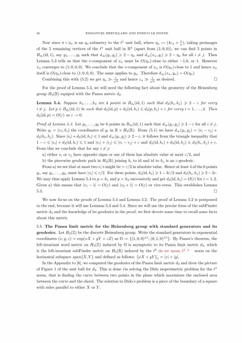
Transcript of Nilpotent groups, asymptotic cones and subfinsler geometry
NILPOTENT GROUPS, ASYMPTOTIC CONES AND SUBFINSLER GEOMETRY
EMMANUEL BREUILLARD AND ENRICO LE DONNE
Abstract. We give an estimate of the speed of convergence of Cayley graphs of general finitely
generated nilpotent groups towards their asymptotic cone. This yields an error term in the asymp-
totics for the volume of large balls, namely |B(n)| = cnd + O(nd−α), where the exponent α > 0 in
the error term depends only on the nilpotency class. Conjecturally this holds for α = 1. We relate
this conjecture to other well-known conjectures in subRiemannian geometry and show that abnormal
geodesics play an important role. We also study in some detail the geometry of the Heisenberg group
(equipped with the Pansu metric) and show that our results are sharp for 2-step groups by giving an
example for which the speed of convergence to the asymptotic cone is no faster than n− 12 .
Contents
1. Introduction 1
2. SubFinsler metrics and dilations on nilpotent Lie groups 5
3. Approximation by horizontal paths and discretization of continuous geodesics 14
4. Proofs of the main results 17
5. Sharpness of the error terms for step-2 groups and the Burago-Margulis conjecture 22
6. Volume of Cayley spheres, regularity of subFinsler spheres and other open problems 31
References 35
1. Introduction
Let Γ be a nilpotent group generated by a finite set of elements S. We will assume that 1 ∈ S and
that S = S−1. Following earlier results of Wolf [22], Bass [3], and Guivarc’h [12], Pansu [17] established
in 1983 that the cardinality of the balls Sn = S · . . . · S of radius n for the word metric induced by S
on the Cayley graph of G is asymptotic to cSnd, where cS > 0 is a positive constant depending on S
and d is an integer independent of S and given by the Bass-Guivarc’h formula:
(1.1) d =∑k>1
kdk,
where dk is the rank of the Abelian group Ck(Γ)/Ck+1(Γ), where C1(Γ) = Γ, Ci+1(Γ) = [Γ, Ci(Γ)] for
i > 1, is the central descending series of Γ.
Date: December 7, 2012.1991 Mathematics Subject Classification. 53C17,22E25.Key words and phrases. subRiemannian geometry, polynomial growth, asymptotic cone, nilpotent groups, Gromov-
Hausdorff convergence, abnormal geodesics.
1
2 EMMANUEL BREUILLARD AND ENRICO LE DONNE
Our main result is the following bound on the second term of the asymptotics. Let r be the
nilpotency step of Γ, i.e., the smallest integer such that Cr+1(Γ) = 1.
Theorem 1.1. There is αr > 0 such that
|Sn| = cSnd +OS(n
d−αr ), as n→ ∞
and one can take αr = 23r .
This improves Pansu’s theorem, which gave no error term. When r = 1, i.e. in the Abelian case,
the result holds with α1 = 1; this is well-known and easy to prove (see [9] for an explicit derivation
and for more on the Abelian case). Stoll showed in [19] that if Γ is a 2-step nilpotent group, i.e. when
r = 2, one can also take α2 = 1. Unfortunately his proof breaks down for groups of nilpotency step 3
and higher (see the remark following [19, Lemma 3.3] and the end of subsection 6.4). Nevertheless we
have no example that may rule out the possibility that one could always take αr = 1 for every r. We
discuss this conjecture further in Section 6 and its connection with other well-known open problems in
subRiemannian geometry.
By way of contrast, the error term obtained in Theorem 1.1 admits no analogue in general for
nondiscrete groups of polynomial growth, where the speed can sometimes be arbitrarily slow. A simple
example is given by the group R2 oθ Z, where Z acts by a rotation Rθ whose angle θ is very well
approximable by rationals multiples of 2π but not in πQ. In this example, the error term can be shown
to be arbitrarily bad if θ is chosen carefully (see [6, §8.1]).In [17], Pansu gave a beautiful description of the asymptotic cone of an arbitrary finitely-generated
torsion-free nilpotent group Γ. Let us briefly recall his results. The Malcev closure G of Γ is a simply-
connected nilpotent Lie group in which Γ embeds as a co-compact discrete subgroup (see [18]). On
every simply-connected nilpotent Lie group G, one can modify the Lie product structure in a natural
(yet nonunique) way and obtain the so-called graded group associated to G. Endowed with this new
Lie product (G, ∗) is a graded nilpotent Lie group (also often called Carnot group when endowed
with a subRiemannian or subFinsler metric) in the sense that it admits a one-parameter subgroup of
R-diagonalisable automorphisms. We refer the reader to Section 2 for this construction.
In his work on groups of polynomial growth [10], Gromov observed that if we renormalize the word
metric ρS in the Cayley graph of Γ by a factor 1n , then there is a subsequence such that the balls of any
given radius converge in the Gromov-Hausdorff topology (see [11, chapter 3], [10]). Pansu [17] showed
that the entire sequence converges and that the limit is a certain metric space, the asymptotic cone
of Γ, which can be described as follows. It is the graded Malcev closure (G, ∗) of Γ endowed with a
certain subFinsler ∗-left-invariant metric d∞ (the Pansu limit metric), which is induced in the usual
way from a certain polyhedral norm on the horizontal subspace of the Lie algebra (which is a transverse
to the commutator subalgebra). The unit ball of this norm, which we call hereafter the Pansu limit
norm, is defined as the convex hull of the projections of the generating set S to the horizontal subspace
of (G, ∗). The coefficient cS in the main term of the asymptotics in Theorem 1.1 is the Lebesgue
measure of the unit ball of (G, ∗), where the measure is normalized so that the lattice Γ has co-volume
1. In Section 2, we describe Pansu’s limit norm and the associated subFinsler metric (also known as
Carnot-Caratheodory metric).
ASYMPTOTICS FOR BALLS IN NILPOTENT GROUPS 3
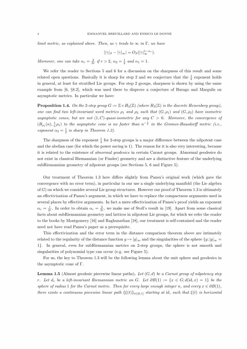
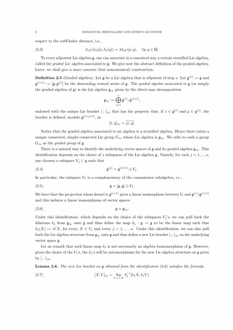
z
yx
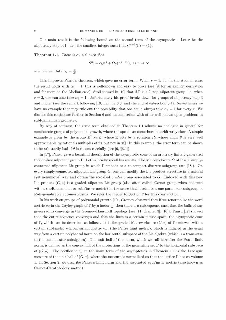
Figure 1. The unit ball for the Pansu limit metric d3 of the Cayley graph of thediscrete Heisenberg group H3(Z) with standard generators (see §5.5 for an explicitformula for d3).
The Gromov-Hausdorff convergence implies that as metric spaces, all the asymptotic cones of Γ
are all isometric to (G, ∗, d∞). Thus (G, ∗, d∞) will be referred to as the asymptotic cone of (Γ, ρS).
In this paper we give an estimate of the speed of convergence towards the asymptotic cone in the
Gromov-Hausdorff metric dGH . Let ρS be the word metric induced by S on Γ, i.e. ρS(x, y) = infn ∈N;x−1y ∈ Sn. For γ ∈ Γ, we set |γ|S = ρS(id, γ) and |γ|∞ = d∞(id, γ) and BS(n) the Cayley ball
centered at id and radius n ∈ N and B∞(R) the ball centered at the origin for d∞ and radius R > 0.
Theorem 1.2. Let Γ be a torsion free nilpotent group with nilpotency class r generated by a finite
subset S (with S = S−1, id ∈ S). Let BS(n) be the ball of radius n in Γ centered at the identity for the
word distance ρS. Let B∞(1) the unit ball at the origin for the Pansu limit metric d∞ on the graded
Malcev closure (G, ∗) of Γ. Then the metric spaces Xn := (BS(n),1nρS) and X∞ := (B∞(1), d∞)
satisfy
dGH(Xn, X∞) = O(n−αr ), as n→ ∞,
for some αr > 0. We can take αr := 23r if r > 2, α2 = 1
2 and α1 = 1.
Theorems 1.1 and 1.2 will follow from the following distance comparison theorem, which compares
the word metric on Γ with the Pansu limit metric on the asymptotic cone of Γ.
Theorem 1.3. (Word metric versus asymptotic metric comparison) For each r ∈ N, there is αr > 0
such that for every finitely-generated torsion-free nilpotent group Γ of nilpotency step r the following
property holds. Let S be a finite generating set for Γ with S = S−1 and 1 ∈ S. Denote by |·|S = ρS(id, ·)the word distance from the identity and by | · |∞ = d∞(id, ·) the distance from the origin in the Pansu
4 EMMANUEL BREUILLARD AND ENRICO LE DONNE
limit metric, as explained above. Then, as γ tends to ∞ in Γ, we have
||γ|S − |γ|∞| = OS(|γ|1−αr∞ ).
Moreover, one can take αr = 23r if r > 2, α2 = 1
2 and α1 = 1.
We refer the reader to Sections 5 and 6 for a discussion on the sharpness of this result and some
related open questions. Basically it is sharp for step 2 and we conjecture that the 12 exponent holds
in general, at least for stratified Lie groups. For step 2 groups, sharpness is shown by using the same
example from [6, §8.2], which was used there to disprove a conjecture of Burago and Margulis on
asymptotic metrics. In particular we have:
Proposition 1.4. On the 2-step group G := Z×H3(Z) (where H3(Z) is the discrete Heisenberg group),
one can find two left-invariant word metrics ρ1 and ρ2 such that (G, ρ1) and (G, ρ2) have isometric
asymptotic cones, but are not (1, C)-quasi-isometric for any C > 0. Moreover, the convergence of
(Bρ1(n),1nρ1) to the asymptotic cone is no faster than n−
12 in the Gromov-Hausdorff metric (i.e.,
exponent α2 = 12 is sharp in Theorem 1.2).
The sharpness of the exponent 12 for 2-step groups is a major difference between the nilpotent case
and the abelian case (for which the power saving is 1). The reason for it is also very interesting, because
it is related to the existence of abnormal geodesics in certain Carnot groups. Abnormal geodesics do
not exist in classical Riemannian (or Finsler) geometry and are a distinctive feature of the underlying
subRiemannian geometry of nilpotent groups (see Sections 5, 6 and Figure 5).
Our treatment of Theorem 1.3 here differs slightly from Pansu’s original work (which gave the
convergence with no error term), in particular in our use a single underlying manifold (the Lie algebra
of G) on which we consider several Lie group structures. However our proof of Theorem 1.3 is ultimately
an effectivization of Pansu’s argument, in which we have to replace the compactness arguments used in
several places by effective arguments. In fact a mere effectivization of Pansu’s proof yields an exponent
αr = 12r . In order to obtain αr = 2
3r , we make use of Stoll’s result in [19]. Apart from some classical
facts about subRiemannian geometry and lattices in nilpotent Lie groups, for which we refer the reader
to the books by Montgomery [16] and Raghunathan [18], our treatment is self-contained and the reader
need not have read Pansu’s paper as a prerequisite.
This effectivization and the error term in the distance comparison theorem above are intimately
related to the regularity of the distance function g 7→ |g|∞ and the singularities of the sphere g; |g|∞ =
1. In general, even for subRiemannian metrics on 2-step groups, the sphere is not smooth and
singularities of polynomial type can occur (e.g. see Figure 5).
For us, the key to Theorem 1.3 will be the following lemma about the unit sphere and geodesics in
the asymptotic cone of Γ.
Lemma 1.5 (Almost geodesic piecewise linear paths). Let (G, d) be a Carnot group of nilpotency step
r. Let de be a left-invariant Riemannian metric on G. Let ∂B(1) := x ∈ G; d(id, x) = 1 be the
sphere of radius 1 for the Carnot metric. Then for every large enough integer n, and every x ∈ ∂B(1),
there exists a continuous piecewise linear path ξ(t)t∈[0,1] starting at id, such that ξ(t) is horizontal
ASYMPTOTICS FOR BALLS IN NILPOTENT GROUPS 5
linear on each interval [ kn ,k+1n ], with derivative of norm at most 1 almost everywhere, and is such that
de(x, ξ(1)) = OG(1n ) as n→ +∞.
In Stoll’s proof of the optimal error term for 2-step groups ([19]), a key lemma consisted in estab-
lishing that in 2-step groups endowed with a subFinsler metric induced from a polyhedral norm, one
can always connect any point on the unit sphere to the origin by a piecewise linear geodesic path with
a uniformly bounded number of breakpoints. So Lemma 1.5, which is in fact not hard to prove, can
be seen as an approximation to Stoll’s lemma, which says that, allowing n breakpoints, one can find
an almost geodesic piecewise linear path (i.e., of total length at most 1 +O(n−1r )) between any point
on the unit sphere and the origin.
This paper is organized as follows. In Section 2, we set some notation and describe Pansu’s construc-
tion of the asymptotic cone. In Section 3 we prove the main technical lemmas about approximating
continuous and discrete geodesic paths including Lemma 1.5. In Section 4, we complete the proofs of
Theorem 1.3, 1.2, and 1.1, in this order. In Section 5, we discuss the sharpness of our results, prove
Proposition 1.4 and discuss in some detail the underlying geometry of the Heisenberg group equiped
with the Pansu limit metric. Finally in Section 6, we discuss some further consequences of our theorems
and state some open questions.
Acknowledgments E.B. is grateful to the ERC for its support through grant GADA-208091. Both
authors would like to thank the MSRI, Berkeley, for perfect working conditions during the Quantitative
Geometry program, when part of this research was conducted. E.B. also thanks Fudan University,
Shanghai, for its hospitality.
2. SubFinsler metrics and dilations on nilpotent Lie groups
2.1. Left-invariant SubFinsler metrics on Lie groups. Let G be a Lie group. Denote by g the
Lie algebra of G considered as the tangent space at the identity element. We will often identify the Lie
algebra with the space of left-invariant vector fields on G.
Suppose a linear subspace V1 ⊂ g and a norm ∥·∥ on V1 are given. Then V1 induces a left-invariant
subbundle ∆ of the tangent bundle of G. Namely, a vector v at a point p ∈ G is an element of ∆
if (Lp)∗v ∈ V1, where Lp : G → G is the left multiplication by p and F ∗ denotes the pull back by a
diffeomorphism F . For such a v, we set ∥v∥ := ∥(Lp)∗v∥ . Such a ∆ is called a horizontal distribution.
The triple (G,∆, ∥·∥) is an example of a subFinsler manifold, cf. [16, 14].
Any subFinsler manifold has an associated distance function, which is called a subFinsler metric
(also known as Carnot-Caratheodory-Finsler metric) and it is defined as follows. One says that an
absolutely continuous curve γ : [a, b] → G, with a, b ∈ R, is horizontal (with respect to ∆) if the
derivative γ(t) belongs to ∆, for almost all t ∈ [a, b]. For such a curve, the value ∥γ(t)∥ is almost
everywhere defined. Hence each horizontal curve γ : [a, b] → G has an associated length defined as
L(γ) :=
∫ b
a
∥γ(t)∥ dt.
Then one defines the subFinsler distance between two points p, q ∈ G as
(2.1) dsF (p, q) := infL(γ) | γ horizontal, from p to q.
6 EMMANUEL BREUILLARD AND ENRICO LE DONNE
Remark. It is possible to show that one may restrict to piecewise linear horizontal paths in the definition
of the length, i.e., to those paths for which γ(t) takes only finitely many values. An explicit proof of
such a fact can be found in [15, Theorem 1.2].
If the Lie algebra generated by V1 is the whole of g, then the function dsF (·, ·) is finite and in fact
defines a geodesic distance that induces the manifold topology on G. This is a particular case of a
theorem by Chow [16, Chapter 2].
The subFinsler metric dsF is said to be subRiemannian if the norm ∥·∥ is an Euclidean norm.
Moreover dsF is said to be Finsler if V1 = g.
SubFinsler metrics are geodesic distances. This means that every two points can be connected by
a geodesic path, i.e., an isometric embedding of an interval. For left-invariant geodesic metrics on Lie
groups, it turns out that the converse also holds, and this is a special case of a more general result due
to Berestovskiı, see [4, Theorem 2, page 892]. Namely:
Theorem 2.2 (Berestovskiı). Let d be a geodesic left-invariant metric on a Lie group that induces the
manifold topology. Then there exist a left-invariant subbundle ∆ and a left-invariant norm ∥·∥ on ∆
such that the distance d is the subFinsler metric associated to ∆ and ∥·∥.
Any two left-invariant Finsler metrics are globally bi-Lipschitz equivalent on G. Things are different
if we compare a Finsler and a subFinsler metric. On the large scale they remain bi-Lipschitz, because,
as it is well-known and easy to check, any two left-invariant geodesic distances on any given locally
compact group are quasi-isometric (see Proposition 2.3 below for a proof). But on small scale, they
can be drastically different. Clearly Riemannian (or Finsler) metrics on G are dominated by subFinsler
metrics up to multiplicative constants. The opposite inequality typically does not hold, but we always
have a lower bound of polynomial type as we now describe.
Assume that V1 together with all brackets of order at most r in the elements of V1 span g linearly.
Let de be any Riemanian metric on G. The Ball-Box Theorem (e.g. [16, Theorem 2.4.2]) implies that,
for any compact set K ⊂ G, there exists a constant C such that
1
C(dsF (id, x))
r 6 de(id, x) 6 CdsF (id, x), ∀x ∈ K.
In particular, we have
(2.2) dsF (id, x) = O(de(id, x)1r ), as x→ 0.
We now record the well-known fact that left-invariant quasi-geodesic metrics on a group G are
always quasi-isometric. Recall that a metric space (X, d) is said to be quasi-geodesic if there exist
constants C > 0 and L > 1 such that every two points in X can be join with a (L,C)-quasi-arc. In
other words, for all x, x′ ∈ X, there exist k ∈ N and x0, x1, . . . , xk ∈ X such that x0 = x, xk = x′,
d(xi−1, xi) 6 C, for i = 1, . . . , k, and∑k
i=1 d(xi−1, xi) 6 Ld(x, x′) + C.
Proposition 2.3. Let d and d′ be two quasi-geodesic left-invariant distances on a locally compact group.
Assume that d and d′ are locally bounded (i.e. bounded on compact sets) and proper (i.e. g 7→ d(id, g)
is a proper map). Then there exist constants c > 0 and L > 1 such that L−1d− c < d′ < Ld+ c.
Proof. Since d is quasi-geodesic, there are two constants C1 > 0 and L1 > 1 with the following property.
Given any group element g, we may find g1, ..., gn such that d(id, gi) 6 C1 for all i and g = g1 · . . . · gn,
ASYMPTOTICS FOR BALLS IN NILPOTENT GROUPS 7
while∑n
1 d(id, gi) 6 L1d(id, g) + C1. Grouping some gi’s together if necessary, we may assume that
C1/2 6 d(id, gi). Hence n 6 2L1
C1d(id, g) + 2. But then by our assumptions of local boundedness and
properness, all gi’s lie in a fixed compact subset of the group and thus d′(id, gi) is uniformly bounded
say by some constant C > 0. Then d′(id, g) 6∑n
1 d′(id, gi) 6 Cn 6 Ld(id, g) + c for L =
2CL1
C1
and c = 2C. The proposition follows by exchanging the roles of d and d′ and using the assumed left
invariance.
The above applies in particular to Finsler and subFinsler left-invariant metrics on Lie groups.
2.4. Stratified Lie algebras and Carnot groups. A special role in subFinsler geometry is played
by those Lie groups whose Lie algebra admits a stratification. We say that a Lie algebra g admits an
s-step stratification, with s ∈ N, if there exist vector subspaces V1, · · · , Vs ⊆ g, such that
g = V1 ⊕ · · · ⊕ Vs,
[Vj , V1] = Vj+1, for 1 6 j 6 s− 1, with Vs = 0, and [Vs, V1] = 0.Here we are using the following notation. Given two vector subspaces V , W of a Lie algebra g,
the set [V,W ] is the vector subspace generated by the commutators of the form [v, w] with v ∈ V and
w ∈ W . The vector subspaces V1, · · · , Vs in the definition of a stratification of an algebra are called
the strata of the stratified Lie algebra g.
Note that every stratified Lie algebra is nilpotent, with nilpotency class (or step) s. Observe further
that the commutator subalgebra [g, g] coincides with V2⊕ · · ·⊕Vs and thus that V1 is in bijection with
the abelianization g/[g, g] via the projection map onto the V1 component. Similarly, for every i, the
i-th term g(i) in the central descending series of g, coincides with Vi ⊕ . . .⊕ Vs.
Note that the first stratum V1 completely determines the other strata. We also remark that every
linear subspace in direct sum with [g, g] generates g, but that it may not always give rise to a stratifica-
tion of g (exercise). One can show that any two stratifications on a given Lie algebra g are isomorphic
in the sense that there is a linear automorphism of g exchanging them (take the change of coordinates
between the two direct sum decompositions).
Let G be a stratified group, i.e., a connected, simply-connected Lie group with stratified Lie algebra
g. In such a group the first stratum V1 generates g. Hence, if V1 is equipped with a norm, we consider
the subFinsler distance dsF (·, ·). The metric space (G, dsF ) is called Carnot group.
One peculiarity of Carnot groups is that they admits dilations in the following sense. For each
λ ∈ R, the algebra-dilation δλ : g → g is defined linearly by imposing δλ(X) := λjX, for every X ∈ Vj
and every j = 1, . . . , s. If λ = 0, then δλ is an automorphism of g. Since the Lie group G is simply-
connected, the dilation induces a unique automorphism on the group, which we still denote by δλ and
call the group-dilation.
Since G is nilpotent and simply-connected, the exponential map exp : g → G is a diffeomorphism.
Thus, group-dilations δλ can be equivalently defined as δλ(p) = exp δλ exp−1(p), for all λ ∈ Rand p ∈ G. Note that λ 7→ δλ, as a map from the positive reals to the group of automorphisms of
G yields a one-parameter group. Since δλ stretches vectors in the horizontal distribution by λ, then
Length(δλ γ) = λLength(γ), for each horizontal curve γ. Hence, δλ is a dilation by a factor of λ with
8 EMMANUEL BREUILLARD AND ENRICO LE DONNE
respect to the subFinsler distance, i.e.,
(2.3) dsF (δλ(p), δλ(q)) = λdsF (p, q), ∀p, q ∈ G.
To every nilpotent Lie algebra g, one can associate in a canonical way a certain stratified Lie algebra,
called the graded Lie algebra associated to g. We give now the abstract definition of the graded algebra.
Later, we shall give a more concrete (but noncanonical) construction.
Definition 2.5 (Graded algebra). Let g be a Lie algebra that is nilpotent of step s. Let g(1) := g and
g(i+1) := [g, g(i)] be the descending central series of g. The graded algebra associated to g (or simply
the graded algebra of g) is the Lie algebra g∞ given by the direct-sum decomposition
g∞ :=s⊕
i=1
g(i)/g(i+1),
endowed with the unique Lie bracket [·, ·]∞ that has the property that, if x ∈ g(i) and y ∈ g(j), the
bracket is defined, modulo g(i+j+1), as
[x, y]∞ = [x, y].
Notice that the graded algebra associated to an algebra is a stratified algebra. Hence there exists a
unique connected, simply-connected Lie group G∞ whose Lie algebra is g∞. We refer to such a group
G∞ as the graded group of g.
There is a natural way to identify the underlying vector spaces of g and its graded algebra g∞. This
identification depends on the choice of s subspaces of the Lie algebra g. Namely, for each j = 1, ..., s,
one chooses a subspace Vj ⊂ g such that
(2.4) g(j) = g(j+1) ⊕ Vj .
In particular, the subspace V1 is a complementary of the commutator subalgebra, i.e.,
(2.5) g = [g, g]⊕ V1.
We have that the projection whose kernel is g(i+1) gives a linear isomorphism between Vi and g(i)/g(i+1)
and this induces a linear isomorphisms of vector spaces:
(2.6) g ≃ g∞.
Under this identification, which depends on the choice of the subspaces Vj ’s, we can pull back the
dilations δλ from g∞ onto g and thus define the map δλ : g → g to be the linear map such that
δλ(X) := λjX, for every X ∈ Vj and every j = 1, . . . , s. Under this identification, we can also pull
back the Lie algebra structure from g∞ onto g and thus define a new Lie bracket [·, ·]∞ on the underlying
vector space g.
Let us remark that each linear map δλ is not necessarily an algebra homomorphism of g. However,
given the choice of the Vi’s, the δλ’s will be automorphisms for the new Lie algebra structure on g given
by [·, ·]∞.
Lemma 2.6. The new Lie bracket on g obtained from the identification (2.6) satisfies the formula
(2.7) [X,Y ]∞ = limλ→+∞
δ−1λ [δλX, δλY ].
ASYMPTOTICS FOR BALLS IN NILPOTENT GROUPS 9
Consequently [δλX, δλY ]∞ = δλ[X,Y ]∞ for all X,Y ∈ g.
Proof. Indeed, since the Vj ’s are a direct decomposition of g, it suffices to show (2.7) for X ∈ Vi and
Y ∈ Vj , for some i, j. In this case, we have that
[X,Y ] = Zi+j + Zi+j+1 + . . .+ Zs,
for some vectors Zk ∈ Vk. Hence
δ−1λ [δλX, δλY ] = δ−1
λ [λiX,λjY ]
= λi+jδ−1λ (Zi+j + Zi+j+1 + . . .+ Zs)
= Zi+j + λ−1Zi+j+1 + . . .+ λi+j−sZs,
which goes to Zi+j , as λ→ ∞. The proof of (2.7) is concluded by observing that Zi+j is a vector that
represent [X,Y ] modulo g(i+j+1).
Finally note that identifying G with g and G∞ with g∞ via the exponential map, the identification
(2.6) also yields an identification at the group level:
(2.8) G ≃ G∞,
which is a diffeomorphism, but not a group isomorphism. Under this identification, the underlying
manifold of the Lie group G can be given a new Lie group structure by pulling back the Lie group
structure of G∞. This Lie structure is also the one induced by the new Lie bracket [X,Y ]∞ on g. In
order to distinguish it from the original Lie product x · y, we will denote the new Lie product on G
obtained in this way by x ∗ y.
2.7. The Campbell-Baker-Hausdorff formula. Suppose G is simply connected nilpotent Lie group
with Lie algebra g and we have chosen subspaces Vi’s as in (2.4). Choose a basis (e1, . . . , en) of g which is
adapted to the direct sum decomposition g = ⊕iVi. The Campbell-Baker-Hausdorff formula allows one
to express the exponential coordinates of the product of two elements of G in terms of the coordinates
of each factor. Given an index i ∈ [1, n], let di be the degree of ei, namely the integer such that ei ∈ Vdi .
For α = (α1, . . . , αn) ∈ Nn a multi-index, we set xα := xα11 · . . . · xαn
n and dα := d1α1 + . . .+ dnαn. We
have for some constants Cα,β ∈ R
Campbell-Baker-Hausdorff formula:
(x · y)i = xi + yi +∑
α,β | dα>1,dβ>1,dα+dβ6di
Cα,βxαyβ .
The new Lie product x∗y defined in the previous subsection with the help of the identification (2.8)
then takes the following simple form (we have chopped the terms with dα + dβ < di):
(x ∗ y)i = xi + yi +∑
α,β | dα>1,dβ>1,dα+dβ=di
Cα,βxαyβ .
10 EMMANUEL BREUILLARD AND ENRICO LE DONNE
2.8. Homogeneous quasi-norms and a lemma of Guivarc’h. Suppose G is a stratified nilpotent
Lie group with Lie algebra g and stratification g = ⊕iVi. Let δλ as above be the one parameter group
of dilations. A non-negative continuous function | · | on G is called a homogeneous quasi-norm if it
satisfies the two axioms: |x| = 0 if and only if x = id, and |δλ(x)| = λ|x| for every λ > 0 and x ∈ G.
Here are two typical examples:
a) a left-invariant subFinsler metric dsF on G with horizontal subspace V1,
b) the function |x| := maxi ci|xi|1/di for any choice of constants ci > 0 (in the notation of subsection
2.7).
The following is a simple observation:
Lemma 2.9. Any two homogeneous quasi-norms | · |1 and | · |2 on G are equivalent in the sense that
there is a constant C > 0 such that 1C | · |1 6 | · |2 6 C| · |1.
When applied to the above two examples of homogeneous quasi-norms, this lemma becomes an
instance of the ball-box principle for Carnot groups.
When the group G is not stratified, it turns out that this ball-box principle remains true under
the identification (2.8), even though the group structures on G and G∞ are not the same. This was
first observed by Guivarc’h in [12]. Using the Campbell-Baker-Hausdorff formula he showed that, even
when G is not stratified, given any choice of subspaces Vi’s as in (2.4), one can always find constants
ci > 0 such that |x| := maxi ci|xi|1/di satisfies |x · y| 6 |x|+ |y|+ 1. As a consequence, he proved the
following comparison theorem:
Proposition 2.10 (Guivarc’h). Let G be a simply connected nilpotent Lie group with Lie algebra g
and U a bounded symmetric neighborhood of id in G. Let ρU (x, y) := infn ∈ N;x−1y ∈ Un be the
word metric induced by U . Let g = ⊕iVi a decomposition as in (2.4) and set |x| = max |xi|1/di . Then
there are constants C,L > 0 such that
1
LρU (id, x)− C 6 |x| 6 LρU (id, x) + C
For the proof, we refer the reader to Guivarc’h thesis [12], or to [6, Theorem 3.7].
2.11. Geodesic left-invariant distances on nilpotent Lie groups. Let us now turn to simply-
connected nilpotent Lie groups and compare subFinsler metrics on them. Let dsF be a left-invariant
subFinsler metric on a simply-connected nilpotent Lie group G. The projection map π : g → g/[g, g]
can be viewed as a map from G to g/[g, g] by precomposing it by the inverse of the exponential map
(which we recall is a diffeomorphism).
Let ∆ be the horizontal distribution for dsF and let V1 := ∆id be the horizontal space at the
identity. Since dsF is finite, we have that V1 is bracket generating, i.e., V1 generates the whole Lie
algebra. Hence π(V1) = g/[g, g], since g/[g, g] is an Abelian algebra. We consider the norm ∥·∥ab on
g/[g, g] whose unit ball is the image in g/[g, g] under π|V1 of the unit ball of ∥·∥ in V1.
Then we have:
Lemma 2.12 (π is a submetry). The projection map π : G→ g/[g, g] is a group homomorphism (i.e.
π(xy) = π(x) + π(y)) and a distance nonincreasing submetry between G metrized with dsF and the
ASYMPTOTICS FOR BALLS IN NILPOTENT GROUPS 11
normed vector space g/[g, g] endowed with the norm ∥·∥ab. This means that the image of any r-ball on
(G, dsF ) is an r-ball on (g/[g, g], ∥·∥ab).
Proof. The identity π(xy) = π(x) + π(y) follows from the Campbell-Baker-Hausdorff formula, which
tells us that exp−1(xy) = exp−1(x) + exp−1(y) modulo g(2).
Given r > 0 and g ∈ G, we need to show that π(BsF (g, r)) = B∥·∥ab(π(g), r). From the left
invariance of dsF , we may assume that g = id. By definition of ∥·∥ab, we have ∥π(x)∥ab 6 ∥x∥ for every
x ∈ g. Integrating this inequality along a horizontal path connecting id and h, it follows immediately
that ∥π(h)∥ab 6 dsF (id, h) for every h ∈ G. So π does not increases distances and we have one inclusion
π(BsF (id, r)) ⊂ B∥·∥ab(0, r).
Moreover if X ∈ g satisfies ∥π(X)∥ab 6 r, then, by definition of the norm ∥·∥ab, there exists
X ∈ V , such that ∥X∥ 6 r. Then dsF (id, exp(X)) 6 r, because exp(tX)t∈[0,1] is a horizontal path
connecting id and exp(X) with length at most r. Finally π(exp(X)) = π(X), so we have proved the
opposite inclusion B∥·∥ab(0, r) ⊂ π(BsF (id, r)).
Remark. Under the identification (2.8) the group G is endowed with a new Lie product ∗. The two
projection maps on G and G∞ agree, because they do so at the Lie algebra level. It follows that π is
also a group homomorphism for the ∗ product, namely π(x ∗ y) = π(x) + π(y).
We will also want to consider ∗-left-invariant subFinsler metrics on G. Although the two Lie
products are typically different (and sometimes not even isomorphic), the associated subFinsler metrics
are comparable, namely:
Proposition 2.13 (left and ∗-left-invariant metrics are comparable). Let G be a simply-connected
nilpotent Lie group and d1 and d2 be two subFinsler metrics on G and suppose that, for each i = 1, 2,
di is either left invariant or ∗-left invariant. Then there are constants C > 0 and L > 1 such that
L−1d1(id, g)− C < d2(id, g) < Ld1(id, g) + C for all g ∈ G.
Proof. If both di are left invariant, or both di are ∗-left invariant, then Proposition 2.3 applies. So we
can assume that say d2 is the ∗-left-invariant subFinsler metric with horizontal subspace the subspace
V1 used in the construction of the identification (2.6) and that d1 is a left-invariant word metric on G.
Then this is precisely the result of Guivarc’h quoted in Proposition 2.10.
A natural question is to ask for a finer comparison between subFinsler metrics. We will say that
d1 and d2 are asymptotic if d1(id,g)d2(id,g)
tends to 1 as g tends to infinity in the group. The following
gives a simple criterion for when two subFinsler metric (be them left invariant or ∗-left invariant) areasymptotic.
Proposition 2.14 (Asymptotic metrics). Two left-invariant subFinsler metrics d1 and d2 are asymp-
totic if and only if the respective projections to g/[g, g] of the unit balls of the norms coincide.
Proof. The ‘only if’ part is the easier half of the statement and follows easily from Lemma 2.12, which
reduces the question to when two norms on a vector space are asymptotic, and this happens if and only
if they are identical of course. The ‘if’ part is harder and we will in fact prove a stronger statement
with error term in Proposition 4.1 below.
12 EMMANUEL BREUILLARD AND ENRICO LE DONNE
2.15. The asymptotic cone of a discrete nilpotent group. We now pass to discrete nilpotent
groups and explain Pansu’s description of their asymptotic cone.
According to a well-known theorem of Malcev ([18, chapter 2]), every torsion-free finitely-generated
nilpotent group Γ is isomorphic to a discrete cocompact subgroup in a connected, simply-connected,
and nilpotent Lie group G. The Lie group G is uniquely determined by Γ and is called the Malcev
closure of Γ.
Let π : G → g/[g, g] be the projection homomorphism (see §2.11). Recall that π is a group
homomorphism (cf. Lemma 2.12), and so in particular π(Γ) is a subgroup of g/[g, g]. Since Γ is
co-compact in G, π(Γ) must also be co-compact in g/[g, g] and thus be a discrete lattice of full rank
there.
Let S be a finite and symmetric generating set for Γ. Consider the image of S under the projection
map π, then take its convex hull B in g/[g, g]. So
B = ConvexHullπ(S).
It is clear that B has nonempty interior. Indeed, otherwise B would be contained in a proper subspace
of g/[g, g], but π(S) generates the lattice of full rank π(Γ) in g/[g, g], hence cannot be contained in
a proper vector subspace. Moreover B is symmetric with respect to the origin, since we assumed
S = S−1. Therefore B is a symmetric convex body with nonempty interior and we can define ∥·∥ to be
the norm on g/[g, g] for which the set B is the unit ball. We will call this norm the Pansu limit norm.
Recall that g/[g, g] is the first stratum of the graded algebra g∞ of g. Let G∞ be the graded group of
g. We call G∞ the graded Malcev closure of Γ. Hence the triple (G∞, g/[g, g], ∥·∥) induces a subFinsler
distance d∞ on the group G∞ and the metric space (G∞, d∞) is a Carnot group. We will call d∞ the
Pansu limit metric.
Recall that S induces on Γ a (left-invariant) word metric ρS defined by setting ρS(id, γ) := infn ∈N; γ ∈ Sn. We can now state:
Theorem 2.16 (Pansu [17]). The sequence of pointed metric spaces (Γ, 1nρS , id) converges in the
Gromov-Hausdorff topology to the Carnot group (G∞, d∞, id). In particular all asymptotic cones of
(Γ, ρS) are isometric to (G∞, d∞).
For the Gromov-Hausdorff topology, we refer the reader to Gromov’s book [11] and to his paper
[10]. Let us only recall the definition. A sequence of pointed metric spaces (Xn, dn, xn) is said to
converge to (X, d, x) if there is εn → 0 such that, for every R > 1, the sequence of bounded metric
spaces (BXn(xn, R + εn), dn) converges to (BX(x,R), d) in the Gromov-Hausdorff topology. Now the
Gromov-Hausdorff metric is a distance on the set of (bounded) metric spaces (X, dX) and (Y, dY )
defined as follows:
dGH(X,Y ) = infdH,Z(X,Y );Z = X ⊔ Y, dZ admissible,
where Z is the disjoint union of X and Y and dZ is an admissible metric on Z, namely a distance
function, which restricts to dX on X and to dY on Y . Here dH,Z is the Hausdorff distance on compact
subsets of Z, namely the smallest r > 0 such that X lies in the r-neighborhood of Y and Y lies in the
r-neighborhood of X.
ASYMPTOTICS FOR BALLS IN NILPOTENT GROUPS 13
We will not give here the definition of asymptotic cones, and will refer the reader to standard
expositions, such as in [21], and also to [11, chapter 3]. The asymptotic cone of a metric space (X, d) is
another metric space (Y, d∞), which roughly speaking is the limit of the original metric space “viewed
from very far”. The construction of the limit typically depends on a choice and is not canonical (a
choice of a non principal ultrafilter). However, if the sequence of pointed metric spaces (X,x, 1nd)
converges in the Gromov-Hausdorff topology to (Y, d∞), then all limits obtained in the asymptotic
cone construction are isometric to (Y, d∞) and then one can speak of the asymptotic cone of (X, d).
We will give now a reformulation of Pansu’s theorem, which makes no mention of asymptotic cones,
but takes the form of a distance comparison theorem between ρS and the subFinsler distance d∞, when
viewed on G after identifying G and G∞ via (2.8). Recall (see the discussion after Definition 2.5) that
any choice of supplementary subspaces Vi’s of g(i+1) inside g(i) gives rise to a natural identification
between g and g∞ and thus between G and G∞. In particular G is then endowed with a new Lie
product ∗ and d∞ becomes a ∗-left-invariant subFinsler metric on G. Theorem 2.16 can be deduced
easily from the following result:
Theorem 2.17 (Pansu [17]). As γ ∈ Γ tends to infinity, we have:
ρS(id, γ)
d∞(id, γ)→ 1
Remark. In Theorem 2.17 we may have replaced d∞ (which is a ∗-left-invariant metric) by the associated
left-invariant metric with the same norm on the same horizontal subspace V1. Indeed this is an instance
of Proposition 2.14 above. Also the theorem holds regardless of the choice of the Vi’s used to identify
G with G∞.
Remark. We will give a full proof below of Theorem 2.17. In fact our proof will give an error term and
yield Theorem 1.3, our main technical result.
Another interesting metric associated to the word metric on Γ is the following one, which we will
call the Stoll metric relative to (Γ, ρS), because Stoll proved in [19] that in 2-step nilpotent groups,
it lies at a bounded distance from the word metric. The Stoll distance of g ∈ G from the identity is
defines as
d(id, g) := inf|t1|+ ...+ |tn|; g = st11 · . . . · stnn , n ∈ N, s1, . . . , sn ∈ S, t1, . . . , tn ∈ R
The following is clear (either directly or by invoking Berestowski’s theorem 2.2):
Lemma 2.18. The Stoll metric d(·, ·) coincides with the left-invariant subFinsler metric induced by
the norm whose unit ball is the convex hull of S in the Lie algebra Lie(G) and with left-invariant
distribution induced by the subspace spanned by S in Lie(G). In particular (by Proposition 2.14 and
Theorem 2.17) we also have ρS(id,γ)d(id,γ) → 1 as γ ∈ Γ tends to ∞.
In fact in [19, Theorem 4.5], Stoll proved the following:
Theorem 2.19 (Stoll). Suppose G is a 2-step simply-connected nilpotent Lie group and Γ a lattice in
it generated by a symmetric generating set S. Let ρS be the word metric on Γ and d be the Stoll metric
on G. Then there is C > 0 such that for all γ ∈ Γ
|d(id, γ)− ρS(id, γ)| 6 C.
14 EMMANUEL BREUILLARD AND ENRICO LE DONNE
Whether this continues to hold in arbitrary step remains an open problem.
3. Approximation by horizontal paths and discretization of continuous geodesics
We will need a well-known and simple lemma about perturbations of controlled paths in Lie groups.
If the derivatives of two paths in V1 are close in L2, then their horizontal lifts are also close.
Lemma 3.1. Let G be a Lie group, let ∥·∥ be some norm on the Lie algebra of G and let de(·, ·) be a
Riemannian metric on G. Then for every L > 0 there is a constant C = C(de, ∥·∥ , L) > 0 with the
following property. Assume ξ1, ξ2 : [0, 1] → G are two piecewise smooth paths in the Lie group G with
ξ1(0) = ξ2(0) = id. Let ξ′i ∈ Lie(G) be the tangent vector pulled back at the identity by a left translation
of G. Assume that supt∈[0,1] ∥ξ′i(t)∥ 6 L, and that ∥ξ′1(t)− ξ′2(t)∥L2([0,1]) 6 ε. Then
de(ξ1(1), ξ2(1)) 6 Cε.
Proof. Note that the paths ξ1 and ξ2 live in a bounded region of G determined by L. For simplicity
of exposition we may assume that such a region is contained in a single coordinate chart. On it the
Riemannian distance is bi-Lipschitz to the Euclidean norm ∥·∥e on the coordinates, thus we may as
well consider the distance associated to this norm instead of de.
We can differentiate and have, for suitable constants C1, C2, K1, and K2,
d
dt∥ξ1(t)− ξ2(t)∥2e = 2⟨ d
dt(ξ1(t)− ξ2(t)), ξ1(t)− ξ2(t)⟩(3.1)
6 2 ∥ξ1(t)− ξ2(t)∥e
∥∥∥∥ ddt (ξ1(t)− ξ2(t))
∥∥∥∥e
(3.2)
= 2 ∥ξ1(t)− ξ2(t)∥e ∥ξ1(t) · ξ′1(t)− ξ2(t) · ξ′2(t)∥e(3.3)
6 2 ∥ξ1(t)− ξ2(t)∥e (∥ξ1(t) · ξ′1(t)− ξ1(t) · ξ′2(t)∥e + ∥ξ1(t) · ξ′2(t)− ξ2(t) · ξ′2(t)∥e)(3.4)
6 2 ∥ξ1(t)− ξ2(t)∥e (C1 ∥ξ′1(t)− ξ′2(t)∥e + C2 ∥ξ1(t)− ξ2(t)∥e)(3.5)
6 K1 ∥ξ1(t)− ξ2(t)∥2e +K2 ∥ξ′1(t)− ξ′2(t)∥2e(3.6)
where, after the triangle inequality, we have used the fact that the map (g, v) → g ·v is locally Lipschitz
in both variables and then the inequality 2ab 6 a2 + b2.
Thusdf
dt6 K1f(t) + α(t),
where f(t) = ∥ξ1(t)− ξ2(t)∥2e and α(t) = K2 ∥ξ′1(t)− ξ′2(t)∥2e. Applying Gronwall’s lemma (or just
noting that the derivative of e−K1tf(t) is at most e−K1tα(t)), we get for t ∈ [0, 1]
f(t) 6 e−K1t
∫ t
0
e−K1sα(s)ds 6 K2eK1 ∥ξ′1(t)− ξ′2(t)∥
2L2([0,1]) ,
and the result follows.
Let G be a simply connected nilpotent Lie group, (δt)t a one-parameter subgroup of dilations as
described in Section 2 and let ∗ be the new Lie product on G associated to the Lie bracket [·, ·]∞obtained from the original one by setting [x, y]∞ := limt→+∞ δ 1
t[δt(x), δt(y)]. Let V1 be the first
eigenspace of δt, which is a subspace transverse to [G,G]. We set V1 as our horizontal subspace. Let
ASYMPTOTICS FOR BALLS IN NILPOTENT GROUPS 15
d∞ be some ∗-left-invariant subFinsler metric on G, with horizontal subspace V1. Finally we take a
fixed ∗-left-invariant Riemannian metric de on G, we also fix a norm ∥·∥ on the Lie algebra g and we
set |g|∞ = d∞(id, g).
Lemma 3.2. Given C > 1, there is D = D(C,G) > 0 such that the following holds. Let n ∈ N and
s, t > 0 such that ns 6 Ct. Let x1, ..., xn be n elements of G with |xi|∞ 6 s, then
de(δ 1t(x1 ∗ . . . ∗ xn), δ 1
t(π1(x1) ∗ . . . ∗ π1(xn)) 6 D
ns2
t2,
and
de(δ 1t(x1 · . . . · xn), δ 1
t(x1 ∗ . . . ∗ xn)) 6 D
ns
t2,
Proof. See [6, Lemma 6.12]. The first estimate is a simple application of Lemma 3.1, where the two
paths ξ1 and ξ2 are taken to be piecewise linear with derivative nδ 1t(xi) and nδ 1
t(π1(xi)) respectively on
each interval [ i−1n , i
n ]. Indeed, let (ej) be a basis of Lie(G) adapted to the direct sum V1 ⊕ . . .⊕ Vr. In
particular, for each j there exists dj such that ej ∈ Vdj . For x ∈ G, denote by (x)j the j-th component
of x with respect to the basis. Notice that there exists a constant K > 0 such that |(x)j | 6 K(|x|∞)dj .
This follows from the equivalence of homogeneous quasi-norms (Lemma 2.9). Then, when dj > 2, we
have the following bound
(x)jtdj
6 K
(|x|∞t
)dj
6 K(st
)dj
6 K(st
)2 (st
)dj−2
6 KCr−2(st
)2
.
Therefore, we have∥∥∥nδ 1t(xi)− nδ 1
t(π1(xi))
∥∥∥e=
∥∥∥∥∥∥n∑
j:dj>2
(xi)jtdj
ej
∥∥∥∥∥∥e
6 KCr−2 dim(G)ns2
t2.
Hence, for some constant D > 0 depending only on C and G, we have
de(nδ 1t(xi), nδ 1
t(π1(xi))) 6 D
ns2
t2.
The conclusion follows from Lemma 3.1.
For the second estimate, we use the Campbell-Baker-Hausdorff formula recalled in Subsection 2.7.
First, letting zk = xk+1 · . . . · xn and yk = x1 ∗ . . . ∗ xk−1, we may write by the triangle inequality:
de(δ 1t(x1 · . . . · xn), δ 1
t(x1 ∗ . . . ∗ xn)) 6
n∑k=2
de(δ 1t(yk ∗ xk ∗ zk), δ 1
t(yk ∗ (xk · zk)))
6n∑
k=2
de(δ 1t(xk ∗ zk), δ 1
t(xk · zk)),
where we used the ∗-left invariance of de. Note that |zk|∞ = O(ns). From the Campbell-Baker-
Hausdorff formula we know that for every x, y ∈ G, xy − x ∗ y =∑
i(xy − x ∗ y)iei and
|(xy − x ∗ y)i| 6∑
dα>1,dβ>1,dα+dβ<di
Cα,β |xαyβ |,
16 EMMANUEL BREUILLARD AND ENRICO LE DONNE
and thus, noting that |xi| = O(|x|di∞) and |xα| = O(|x|dα
∞ ), if |x|∞ 6 Cs and |y|∞ 6 Ct,
|(xy − x ∗ y)i| =∑
dα>1,dβ>1,dα+dβ<di
O(|x|dα∞ |y|dβ
∞ ) = OC(stdi−2)
Hence we have shown that if |x|∞ 6 Cs and |y|∞ 6 Ct, then
(3.7) de(δ 1t(xy), δ 1
t(x ∗ y)) = OC(
s
t2)
Applying this to x = xk and y = zk and summing, we finally obtain
de(δ 1t(x1 · . . . · xn), δ 1
t(x1 ∗ . . . ∗ xn)) = OC(
ns
t2),
as desired.
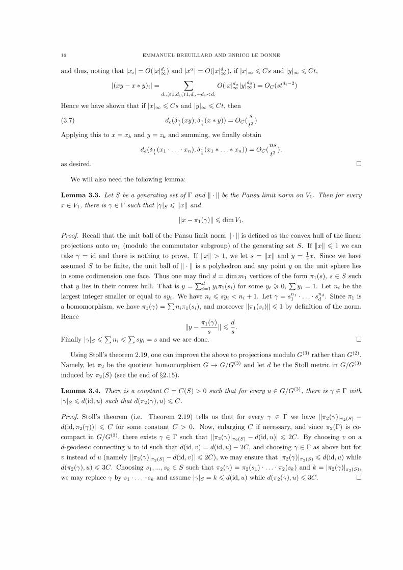
We will also need the following lemma:
Lemma 3.3. Let S be a generating set of Γ and ∥ · ∥ be the Pansu limit norm on V1. Then for every
x ∈ V1, there is γ ∈ Γ such that |γ|S 6 ∥x∥ and
∥x− π1(γ)∥ 6 dimV1.
Proof. Recall that the unit ball of the Pansu limit norm ∥ · ∥ is defined as the convex hull of the linear
projections onto m1 (modulo the commutator subgroup) of the generating set S. If ∥x∥ 6 1 we can
take γ = id and there is nothing to prove. If ∥x∥ > 1, we let s = ∥x∥ and y = 1sx. Since we have
assumed S to be finite, the unit ball of ∥ · ∥ is a polyhedron and any point y on the unit sphere lies
in some codimension one face. Thus one may find d = dimm1 vertices of the form π1(s), s ∈ S such
that y lies in their convex hull. That is y =∑d
i=1 yiπ1(si) for some yi > 0,∑yi = 1. Let ni be the
largest integer smaller or equal to syi. We have ni 6 syi < ni + 1. Let γ = sn11 · . . . · snd
d . Since π1 is
a homomorphism, we have π1(γ) =∑niπ1(si), and moreover ∥π1(si)∥ 6 1 by definition of the norm.
Hence
∥y − π1(γ)
s∥ 6 d
s.
Finally |γ|S 6∑ni 6
∑syi = s and we are done.
Using Stoll’s theorem 2.19, one can improve the above to projections modulo G(3) rather than G(2).
Namely, let π2 be the quotient homomorphism G → G/G(3) and let d be the Stoll metric in G/G(3)
induced by π2(S) (see the end of §2.15).
Lemma 3.4. There is a constant C = C(S) > 0 such that for every u ∈ G/G(3), there is γ ∈ Γ with
|γ|S 6 d(id, u) such that d(π2(γ), u) 6 C.
Proof. Stoll’s theorem (i.e. Theorem 2.19) tells us that for every γ ∈ Γ we have ||π2(γ)|π2(S) −d(id, π2(γ))| 6 C for some constant C > 0. Now, enlarging C if necessary, and since π2(Γ) is co-
compact in G/G(3), there exists γ ∈ Γ such that ||π2(γ)|π2(S) − d(id, u)| 6 2C. By choosing v on a
d-geodesic connecting u to id such that d(id, v) = d(id, u) − 2C, and choosing γ ∈ Γ as above but for
v instead of u (namely ||π2(γ)|π2(S) − d(id, v)| 6 2C), we may ensure that |π2(γ)|π2(S) 6 d(id, u) while
d(π2(γ), u) 6 3C. Choosing s1, ..., sk ∈ S such that π2(γ) = π2(s1) · . . . · π2(sk) and k = |π2(γ)|π2(S),
we may replace γ by s1 · . . . · sk and assume |γ|S = k 6 d(id, u) while d(π2(γ), u) 6 3C.
ASYMPTOTICS FOR BALLS IN NILPOTENT GROUPS 17
The above lemma will be useful in our main theorems in order to obtain the exponent 23r instead
of the exponent 12r , which is what one gets by using Lemma 3.3.
We complete this section with the proof of Lemma 1.5 from the Introduction.
Proof of Lemma 1.5. Let π1 be the projection to the first stratum of G, and let γ(t)t∈[0,1] be a
geodesic path connecting the origin to x. We set
xi = δn(γ(i− 1
n)−1γ(
i
n)),
for i = 1, . . . , n. Let ξ(t)t∈[0,1] be the path whose derivative is piecewise constant equal π1(xi)
on each interval [ i−1n , i
n ]. Note that d(id, xi) = 1 and hence ∥π1(xi)∥ 6 1 by Lemma 2.12. Then
ξ(1) = δ 1n(π1(x1) · . . . · π1(xn)) and Lemma 3.2 applies, with s = 1 and t = n, and yields de(ξ(1), x) =
O(n−1).
4. Proofs of the main results
In this section we prove our main theorems.
The following proposition is a simple consequence of Lemma 3.2. Let G be a simply connected
nilpotent Lie group, (δt)t a one-parameter subgroup of dilations as described in Section 2 and let ∗be the new Lie product on G associated to the Lie bracket [·, ·]∞ obtained from the original one by
setting [x, y]∞ := limt→+∞ δ 1t[δt(x), δt(y)]. Let d be some left-invariant geodesic metric on G, let V1
be the first eigenspace of δt, which is a subspace transverse to [G,G]. By Berestovski’s theorem (see
Section 2) d is a subFinsler metric associated to some norm on a subspace of the Lie algebra of G.
Observe that this subspace projects surjectively onto V1 modulo [g, g] (because the horizontal subspace
at the origin for d generates the Lie algebra) and that the projection of the unit ball of this norm on
V1 modulo [g, g] defines a norm ∥ · ∥ on V1. This norm induces a ∗-left-invariant subFinsler metric d∞
on G with horizontal subspace V1. We set the following notation |g| = d(id, g) and |g|∞ = d∞(id, g).
Proposition 4.1 (Comparison of subFinsler metrics). We have:
||g|∞ − |g|| = O(|g|1− 1r ), as |g| → ∞.
Proof. Recall that by Proposition 2.13 we have |g|∞ = O(|g|) and |g| = O(|g|∞), as |g| or |g|∞ → ∞.
We first prove one side of the inequality, namely |g|∞ 6 |g|+ O(|g|1− 1r ). Let t = |g|∞. Since d is left
invariant and geodesic, we may write g = g1 · . . . · gn for some gi in a fixed compact set and n ≃ t,
so that |g| =∑
|gi|. Indeed simply take gi = γ(i − 1)−1γ(i), where γ(t)t∈[0,|g|] is a geodesic path
connecting the origin to g. By Lemma 3.2 we may write,
de(δ 1t(g), δ 1
t(π1(g1) ∗ . . . ∗ π1(gn))) = O(
1
n),
where de is a ∗-left-invariant Riemannian metric on G. Hence recalling (2.2)
d∞(g, π1(g1) ∗ . . . ∗ π1(gn)) = O(t1−1r )
and |g|∞ 6 |π1(g1) ∗ . . . ∗ π1(gn)|∞ + O(t1−1r ). On the other hand |π1(gi)|∞ = ∥π1(gi)∥ 6 |gi| by
definition of the norm ∥ · ∥, hence
|g|∞ 6∑
|gi|+O(t1−1r ) = |g|+O(|g|1− 1
r )
18 EMMANUEL BREUILLARD AND ENRICO LE DONNE
as desired.
We now turn to the reverse inequality. We set this time t = |g| and consider a d∞-geodesic
g = g1 ∗ . . . ∗ gn, where the gi’s are in a fixed compact set, n ≃ t, and∑
|gi|∞ = |g|∞. By definition of
the norm ∥ · ∥ we may find y1, . . . , yn in G such that π1(yi) = π1(gi) and |yi| 6 ∥π1(gi)∥. Now we set
h := π1(g1) ∗ . . . ∗ π1(gn), and y = y1 · . . . · yn and observe that |y| 6∑
|yi| 6∑
∥π1(gi)∥ 6∑
|gi|∞ =
|g|∞. Then applying Lemma 3.2 we get
de(δ 1t(y), δ 1
t(h)) = O(
1
t),
and
de(δ 1t(g), δ 1
t(h)) = O(
1
t).
Hence by the triangle inequality de(δ 1t(g), δ 1
t(y)) = O( 1t ). Recalling (3.7), we have de(δ 1
t(g−1y), δ 1
t(g−1∗
y)) = O( 1t ). Then by the triangle inequality de(id, δ 1t(g−1y)) = O( 1t ) and by (2.2) we get
|δ 1t(g−1y)|∞ = O(t−
1r ).
Finally we obtain the desired bound using Proposition 2.13:
|g| 6 |y|+ |g−1y| 6 |g|∞ +O(|g−1y|∞) 6 |g|∞ +O(|g|1−1r∞ ).
4.2. Proof of Theorem 1.3. In the proof of the previous proposition, we considered in each case a
geodesic connecting g to the identity and we split it into n ≃ |g| pieces and approximate it by piecewise
linear horizontal paths using Lemma 3.2. In the forthcoming proof of Theorem 1.3 below, we will follow
a similar strategy, except that we will split a d∞-geodesic of length t into roughly√t pieces of equal
length, and then take advantage of Lemma 3.3 to find a nearby path inside the discrete group Γ. This
will lead to an error term with αr = 12r , which is slightly worse than the αr = 2
3r that we claimed in
the introduction. We explain how to modify the argument to get the 23r exponent afterwards.
Proof of Theorem 1.3 with exponent 12r . There are two distinct arguments for the lower bound and for
the upper bound. The easier of the two, namely showing the lower bound, follows from Proposition
4.1 above. Indeed, we let d be the Stoll metric (see Lemma 2.18) associated to S on G, namely
the left-invariant subFinsler metric on G induced by the set S by setting d(id, g) = inf|t1| + ... +
|tn|; g = st11 · . . . · stnn , tj ∈ R. For γ ∈ Γ, set |γ| = d(id, γ). Clearly |γ| 6 |γ|S for every γ ∈ Γ.
Moreover the associated ∗-left-invariant subFinsler metric on G induced by the norm on V1 obtained
by projecting the convex hull of S coincides with the asymptotic cone metric d∞. Thus by Proposition
4.1 |γ|∞ 6 |γ|+O(|γ|1−1r∞ ) 6 |γ|S +O(|γ|1−
1r∞ ) as desired (note that we get the better exponent 1
r here
for the lower bound).
We now pass to the upper bound. This will require Lemma 1.5 which we proved in Section 3,
and is about approximating geodesic paths by piecewise linear paths. Let x ∈ G such that |x|∞ = 1
and let t > 1. From Lemma 1.5, we can find, for every n > 1 (large but much smaller than t, to
be determined later), a continuous unit speed piecewise horizontal path ξ(s)s∈[0,1] with ξ(0) = id and
de(x, ξ(1)) = O( 1n ), such that on each [ kn ,k+1n ] the curve ξ(s) is horizontal (recall that de is a fixed
∗-left-invariant Riemannian metric on G). Note that ‘horizontal’ here is to be understood with respect
ASYMPTOTICS FOR BALLS IN NILPOTENT GROUPS 19
to the ∗-left-invariant bundle induced by V1. This means that there are elements y1, ..., yn in V1 on the
unit ball of the Pansu limit norm such that ξ(1) = ( 1ny1) ∗ . . . ∗ (1nyn). We may then apply Lemma 3.3
and find group elements γ1, . . . , γn ∈ Γ such that |γi|S 6 tn and
∥yi −π1(γi)
t/n∥ 6 dimG
t/n.
We let z := ( 1tπ1(γ1)) ∗ . . . ∗ (1tπ1(γn)) and observe that applying Lemma 3.1 yields de(z, ξ(1)) =
OG(1
t/n ). Now by Lemma 3.2 applied to xi = γi, we obtain
de(z, δ 1t(gn)) = O(
n(t/n)2
t2) = O(
1
n),
where gn := γ1 · . . . · γn. Finally
de(x, δ 1t(gn)) = O(
1
t/n) +O(
1
n).
Then setting n ≃ t12 , we obtain the bound de(x, δ 1
t(γ1 · . . . · γn)) = O(t−
12 ). Now suppose γ ∈ Γ
and set t = |γ|∞ and x = δ 1t(γ). Then both |γ|∞ and |γ1 · . . . · γn|∞ are at most O(t), and so we know
by (3.7) that de(δ 1t(γ−1 ∗ gn), δ 1
t(γ−1 · gn)) = O( 1t ). We conclude from the triangle inequality that
de(id, δ 1t(γ−1 · gn)) = O(t−
12 ).
By (2.2), we have that
|δ 1t(γ−1 · gn)|∞ = O(t−
12r ).
Finally, using Proposition 2.13,
|γ|S 6 |gn|S + |γ−1 · gn|S
6 n · tn+O(|γ−1 · gn|∞)
6 t+O(t1−12r ) = |γ|∞ +O(|γ|1−
12r∞ )
and we are done.
Note that the proof actually gave an exponent 1r in the lower bound, and an exponent αr = 1
2r
for the upper bound. However if we repeat the same proof and replace d∞ with the left-invariant
subFinsler metric induced by the projection of S on the first two strata and use Theorem 2.19 (Stoll’s
theorem) and Lemma 3.4 in place of Lemma 3.3, this will allow us to subdivide the geodesic into n ≃ t13
intervals of equal length (instead of√t intervals). Ultimately this will give an element gn ∈ Γ with
|gn|S 6 t and de(x, δ1/t(gn)) = O(t−23 ) and thus an exponent αr = 2
3r in the upper bound. We now
pass to the details.
Let π2 : g → V1 ⊕ V2 be the linear projection modulo g(3). Note that the 2-step Lie algebras g/g(3)
and g∞/g(3)∞ are isomorphic under the identification of g and g∞ given by any choice of Vi’s. Thus V1⊕V2
is given this 2-step Lie algebra structure and then π2 becomes a Lie algebra homomorphism. We can also
view V1⊕V2 as endowed with the associated Lie product. Then π2 becomes a homomorphism defined on
G. Finally we note that π2 respects both Lie products on G, namely π2(xy) = π2(x ∗ y) = π2(x)π2(y).
Now let d be the ∗-left-invariant subFinsler metric on G which is defined exactly as d∞, except that
we consider the linear projection π2 of S to the first two strata V1 ⊕ V2, then take the left-invariant
20 EMMANUEL BREUILLARD AND ENRICO LE DONNE
distribution induced by V1⊕V2. If we endow V1⊕V2 = g/g(3) with the left-invariant metric induced by
the same norm, then π2 becomes a distance non-increasing map (and in fact a submetry) from (G, d)
to V1 ⊕ V2. Abusing notation, we again denote by d this subFinsler metric on V1 ⊕ V2. We will also
abuse notation similarly and continue to denote by d∞ the subFinsler metric on V1 ⊕ V2 which is the
projection of d∞ from G to G/G(3) ≃ V1 ⊕ V2.
Now pick g ∈ G and let t = d(id, g). Let n 6 t to be determined later. Now connect g to
id by a d-geodesic, so that we have g = x1 ∗ . . . ∗ xn with d(id, xi) 6 tn . Let x = δ 1
t(g). Let
ξ = δ 1t(π2(x1)) ∗ . . . ∗ δ 1
t(π2(xn)). Then because of the π2 projection, we gain a little more in the
approximation of x by ξ. Namely (taking any norm on the vector space g) :
(4.1) ||nδ 1t(π2(xi))− nδ 1
t(xi)|| = O(
1
n2)
and thus, applying Lemma 3.1, we obtain
de(x, ξ) = O(1
n2).
Now the projection of Γ on V1 ⊕ V2 ≃ G/G(3) is a discrete co-compact subgroup of G/G(3) and thus
every element u in V1 ⊕ V2 admits an element γ ∈ Γ such that d(u, π2(γ)) 6 C for some constant
C. Recall Lemma 3.4, which is the 2-step analogue to Lemma 3.3 and follows from Stoll’s theorem
(Theorem 2.19), namely:
Lemma 4.3. There is a constant C = C(S) > 0 such that for every u ∈ G/G(3), there is γ ∈ Γ with
|γ|S 6 d(id, u) such that d(π2(γ), u) 6 C.
Apply the lemma to each u = π2(xi) and obtain γi ∈ Γ such that |γi|S 6 tn and d(π2(γi), π2(xi)) 6
C. By left invariance we get d∞(π2(γi), π2(xi)) = O(1) and hence d∞(δ 1t(π2(γi)), δ 1
t(π2(xi))) = O( 1t ).
Since de ≪ d∞, we deduce that
||nδ 1t(π2(xi))− nδ 1
t(π2(γi))|| = O(
1
t/n)
Then consider z := δ 1t(π2(γ1)) ∗ . . . ∗ δ 1
t(π2(γn)) and apply Lemma 3.1 again to obtain:
de(ξ, z) = O(1
t/n)
Now set gn := γ1 · . . . · γn. We have |gn|S 6 n tn = t. On the other hand the second estimate of Lemma
3.2 applied to the γi’s with s = t/n shows that
de(δ 1t(gn), δ 1
t(γ1) ∗ . . . ∗ δ 1
t(γn)) = O(
1
t).
Now applying Lemma 3.1 again exactly as we did in (4.1) yields
de(z, δ 1t(γ1) ∗ . . . ∗ δ 1
t(γn)) = O(
1
n2)
It follows from the triangle inequality that
de(x, δ 1t(gn)) = O(
1
n2) +O(
1
t/n).
ASYMPTOTICS FOR BALLS IN NILPOTENT GROUPS 21
The remainder of the proof is then exactly as before, except we set the value of n to be roughly n ≃ t13
instead of t12 as before. So we have
de(δ 1t(g), δ 1
t(gn)) = O(t−
23 ),
while t = d(id, g) and gn ∈ Γ with |gn|S 6 t. We conclude as before using (3.7) that de(id, δ 1t(g−1gn)) =
O(t−23 ). Then if g ∈ Γ, |g−1gn|S = O(|g−1gn|∞) = O(t−
23r ) so finally |g|S 6 |gn|S + O(t−
23r ) 6
d(id, g) + O(t−23r ). Finally Proposition 4.1 shows that d and d∞ are O(d1−
1r ) away from each other,
hence ||g|S − |g|∞| is also O(|g|1−23r∞ ), and we are done. This ends the proof of Theorem 1.3 with the
exponent 23r .
We remark that the above proof shows that the renormalized Cayley ball δ 1n(BS(n)) converges (in
the Hausdorff metric of compact subsets of G) towards the Pansu limit ball B∞(1) (i.e. the unit ball for
the d∞ metric). We are going to prove that it also converges as metric spaces in the Gromov-Hausdorff
metric and prove Theorem 1.2, which gives an estimate on the speed of convergence.
To this end, observe that given x ∈ B∞(1) and n ∈ N, the proof above builds an element γx ∈ Γ
(denoted gn above) such that |γx|S 6 n and d∞(x, δ 1n(γx)) = O(n−αr ). Similarly Proposition 3.2 shows
that given x = δ 1n(γ) for γ ∈ BS(n), there exists an element yγ ∈ B∞(1) with d∞(x, yγ) = O(n−
1r )
and yγ = δ 1n(π1(s1) ∗ . . . ∗π1(sn)) for some s1, . . . , sn in S such that γ = s1 · . . . · sn. We are now ready
for the proof of Theorem 1.2.
Proof of Theorem 1.2. Let dn = 1nρS be the distance on Xn. Let Z = Xn ⊔X be the disjoint union of
X and Xn and let ϕ : Z → Xn and ψ : Z → X be the surjective maps defined as follows. If α = x ∈ X
we let ψ(α) = α and set ϕ(α) to be the element δ 1n(γx) defined above. While if α = δ 1
n(γ) ∈ Xn for
γ ∈ BS(n), then we set ϕ(α) = α and set ψ(α) to be the element yγ ∈ X defined above.
Next we define a distance on Z = Xn ⊔X which restricts to dn = 1nρS on Xn and to d∞ on X and
is defined for x ∈ X and x′ = δ 1n(γ) ∈ Xn by
d(x, x′) := infα∈Z
dn(x′, ϕ(α)) + d∞(ψ(α), x)+ εn,
where εn is soon to be determined. It is easy to check that this is indeed a distance on Z provided
(4.2) supα,β∈Z
|dn(ϕ(α), ϕ(β))− d∞(ψ(α), ψ(β))| 6 2εn.
Moreover, by construction, d(ϕ(α), ψ(α)) 6 εn and hence dGH(Xn, X) 6 εn by definition of dGH (see
Section 2.15). We now show that (4.2) holds with εn = O(n−αr ) and this will finish the proof of
Theorem 1.2.
We have three kinds of quantities to estimate depending on whether α and β belong to X or
to Xn. However it will be enough to prove the estimate say for α, β ∈ X, provided we show that
dn(α, ϕ ψ(α)) = O(n−αr ) when α ∈ Xn. Both estimates are easy to prove given the definitions with
the help of (3.7).
For dn(α, ϕ ψ(α)) = O(n−αr ), we recall that given γ ∈ BS(n), d∞(yγ , δ 1n(γyγ )) = O(n−αr ) and
that d∞(δ 1n(γ), yγ) = O(n−
1r ). Hence by the triangle inequality d∞(δ 1
n(γyγ ), δ 1
n(γ)) = O(n−αr ). Now
applying (3.7) we get d∞(id, δ 1n(γ−1
yγγ)) = O(n−αr ), and since d∞ and ρS are comparable by Proposition
2.13 we finally obtain dn(id, δ 1n(γyγ )
−1γ) = O(n−αr ) as desired.
22 EMMANUEL BREUILLARD AND ENRICO LE DONNE
The estimate |d∞(x, y)− dn(δ 1n(γx), δ 1
n(γy))| = O(n−αr ) is dealt with in a similar fashion. Namely
recall that d∞(x, δ 1n(γx)) = O(n−αr ). We thus get |d∞(x, y) − d∞(δ 1
n(γx), δ 1
n(γy))| = O(n−αr ). On
the other hand, |d∞(δ 1n(γx), δ 1
n(γy))− d∞(id, δ 1
n(γ−1
x γy))| 6 d∞(δ 1n(γ−1
x ∗ γy), δ 1n(γ−1
x γy)) which is 6de(δ 1
n(γ−1
x ∗γy), δ 1n(γ−1
x γy))1r by (2.2), which in turn is a O(n−
1r ) by (3.7). Finally |d∞(id, δ 1
n(γ−1
x γy))−dn(id, δ 1
n(γ−1
x γy))| = O(n−αr ) by Theorem 1.3, and we are done.
Proof of Theorem 1.1. We first assume that Γ is torsion free and thus embeds in its Malcev closure
G as a discrete co-compact subgroup. The result will follow easily from Theorem 1.3 and Proposition
4.1 above. First, normalize the Haar measure on G so that G/Γ has total volume 1, and let F be
a compact fundamental domain for the action of Γ on G. Let d and d∞ be the left-invariant and
∗-left-invariant subFinsler metrics on G respectively, which are induced from the Pansu limit norm on
V1 associated to S as described in Section 2. Combining Theorem 1.3 and Proposition 4.1, we see that
||γ|S − |γ|| = OS(|γ|1−αr ) for every γ ∈ Γ. Given that F is compact, there must be a constant C > 0
such that SnF ⊂ Bd(n + O(n1−αr )) for all n > 1. And conversely, if g ∈ Bd(n), then there is f ∈ F
such that gf−1 ∈ Γ and we thus get B(n) ⊂ Sn+n1−αrF for every n > 1. Taking the Haar volume of
SnF , we obtain:
volBd
(n−O(n1−αr )
)6 vol(SnF ) 6 volBd
(n+O(n1−αr )
).
On the other hand we can compare Bd and Bd∞ using Proposition 3.2 and conclude that the above
inequality also holds with Bd∞ in place of Bd. However d∞ is admits the scaling property |δt(g)|∞ =
t|g|∞, and thus volBd∞(t) = td volBd∞(1). Observing that with our choice of normalization for the
Haar measure vol(SnF ) = |Sn|, we obtain the desired result with cS = volBd∞(1).
Now a word about the torsion case. As is well-known (see [18, chapter 2]), the set T of torsion
elements in Γ is a finite normal subgroup of Γ and Γ/T is torsion free. In particular, there exists n0 > 1
such that T ⊂ Sn0 . If S is the projection of S in Γ/T , then |Sn| = cSnd +O(nd−αr ). However, on the
one hand |Sn| 6 |SnT | = |Sn||T | and on the other hand |Sn||T | = |SnT | 6 |Sn+n0 |. It follows that
|Sn| = cS |T |nd +O(nd−αr ) as desired.
5. Sharpness of the error terms for step-2 groups and the Burago-Margulis
conjecture
In [1] D. Burago and G.A. Margulis conjectured that any two left-invariant word distances on a
group ρ1 and ρ2 which are asymptotic in the sense that ρ1(id,γ)ρ2(id,γ)
→ 1 as γ → ∞, must be at a bounded
distance from each other, i.e. |ρ1(id, γ) − ρ2(id, γ)| = O(1). Burago proved the conjecture for Rn
and Zn in [7] and Abels and Margulis [2] did so for word metrics in reductive real Lie groups. Krat
proved it for the discrete Heisenberg group in [13] and also for word hyperbolic groups. However it
turned out that their conjecture failed for general discrete nilpotent groups, and the first author gave
a counter-example in [6, §8.2]. In this counter-example the difference |ρ1(id, γ) − ρ2(id, γ)| can be of
order√ρ2(γ).
In this section we recall the counter-example from [6, §8.2] and proceed by proving Proposition
1.4, which is the much stronger statement that although ρ1 and ρ2 are asymptotic and have isometric
asymptotic cones, they are not (1, C)-quasi-isometric for any C > 0 (note that the failure of the
ASYMPTOTICS FOR BALLS IN NILPOTENT GROUPS 23
Burago-Margulis conjecture boils down to the weaker fact that the identity map is not a (1, C)-quasi-
isometry). Recall that a map ϕ : X → Y between two metric spaces (X, dX) and (Y, dY ) is called a
(1, C)-quasi-isometry if dX(a, b)−C 6 dY (ϕ(a), ϕ(b)) 6 dX(a, b)+C, for all a, b ∈ X, and every y ∈ Y
is at distance at most C from some element of ϕ(X).
This will be done by proving that the renormalized Cayley ball are at least n−12 away (instead of the
expected n−1) from the asymptotic cone metric. Hence the sharpness of the exponent 12 in our main
theorem, Theorem 1.3, and in the Gromov-Hausdorff convergence of Theorem 1.2 for step-2 groups.
The counter-example from [6, §8.2] was built as follows. Let G = G(Z) = Z×H3(Z), where H3(Z) isthe 3-dimensional discrete Heisenberg group. We will use exponential coordinates g = (v;x, y, z) for the
element g = exp(vV +xX + yY + zZ) in G, where V,X, Y, Z are the generators of the (4-dimensional)
Lie algebra of G(R) defined by the relations [X,Y ] = Z and all other brackets are zero.
We consider the two left-invariant word metrics ρ1 and ρ2 on G induced by the following choice of
generating set:
Ω1 := (1; 0, 0, 1)±1, (1; 0, 0,−1)±1, (0; 1, 0, 0)±1, (0; 0, 1, 0)±1
gives rise to ρ1, and
Ω2 := (1; 0, 0, 0)±1, (0; 1, 0, 0)±1, (0; 0, 1, 0)±1
gives rise to ρ2.
The abelianization of the Lie algebra g of G(R) is 3-dimensional. We will set the first stratum of
g to be the linear span of V , X and Y . The projections of Ω1 and Ω2 on the abelianization g/[g, g]
coincide. It thus follows from Pansu’s theorem that ρ1 and ρ2 are asymptotic, i.e. ρ1(id,γ)ρ2(id,γ)
converges
to 1 as γ tends to ∞ in G. In particular their asymptotic cones are isometric and coincide with the
Carnot group G(R) endowed with the left-invariant subFinsler metric induced by the convex hull of
π(Ω1) = π(Ω2). Let d∞(·, ·) be this Pansu limit metric on G(R).Observe that although the Pansu limit metrics associated to ρ1 and ρ2 coincide, the corresponding
Stoll limit metrics are different. For ρ2 the Stoll limit metric is precisely d∞, but this is not the case
for ρ1. In view of Stoll’s theorem (see Theorem 2.19), ρ2 and d∞ are at a bounded distance from each
other. This implies that the convergence of the renormalized Cayley balls (Bρ2(id, n),1nρ2) towards
the asymptotic cone (i.e. (Bd∞(id, 1), d∞) is best possible, that is the Gromov-Hausdorff distance is at
most O( 1n )). However this is not the case for ρ1 and we show:
Proposition 5.1. Let X1n = (Bρ1
(id, n), 1nρ1) and X∞ := (Bd∞(id, 1), d∞). Then
dGH(X1n, X∞) >
c√n,
for some c > 0. In particular (G, ρ2) and (G, ρ1) are not (1, C) quasi-isometric for any C > 0 even
though they have isometric asymptotic cones.
To see how the statement about the absence of (1, C)-quasi-isometries follows from the lower
bound on the Gromov-Hausdorff distance, simply observe that if (G, ρ2) and (G, ρ1) where (1, C)-
quasi-isometric for some C > 0, then so would be (G, ρ2) and (G(R), d∞) and we would then have
24 EMMANUEL BREUILLARD AND ENRICO LE DONNE
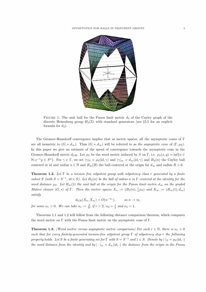
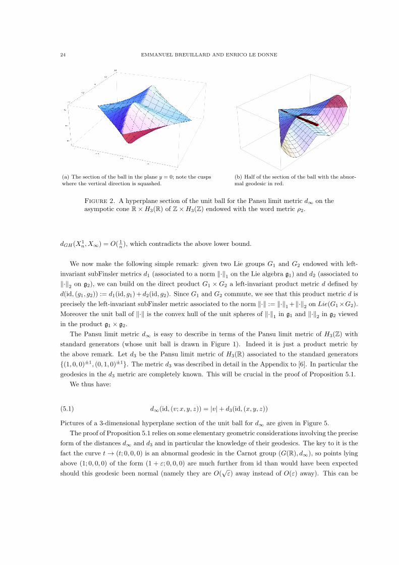
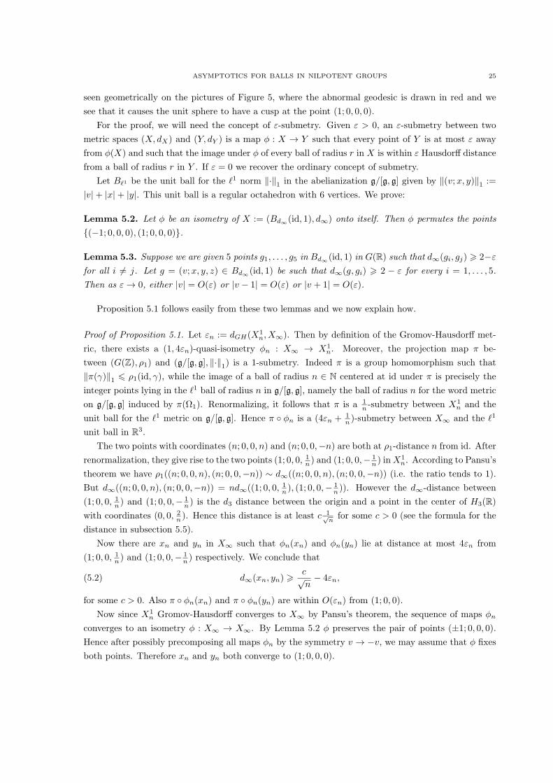
(a) The section of the ball in the plane y = 0; note the cuspswhere the vertical direction is squashed.
(b) Half of the section of the ball with the abnor-mal geodesic in red.
Figure 2. A hyperplane section of the unit ball for the Pansu limit metric d∞ on theasympotic cone R×H3(R) of Z×H3(Z) endowed with the word metric ρ2.
dGH(X1n, X∞) = O( 1n ), which contradicts the above lower bound.
We now make the following simple remark: given two Lie groups G1 and G2 endowed with left-
invariant subFinsler metrics d1 (associated to a norm ∥·∥1 on the Lie algebra g1) and d2 (associated to
∥·∥2 on g2), we can build on the direct product G1 × G2 a left-invariant product metric d defined by
d(id, (g1, g2)) := d1(id, g1)+ d2(id, g2). Since G1 and G2 commute, we see that this product metric d is
precisely the left-invariant subFinsler metric associated to the norm ∥·∥ := ∥·∥1+∥·∥2 on Lie(G1×G2).
Moreover the unit ball of ∥·∥ is the convex hull of the unit spheres of ∥·∥1 in g1 and ∥·∥2 in g2 viewed
in the product g1 × g2.
The Pansu limit metric d∞ is easy to describe in terms of the Pansu limit metric of H3(Z) with
standard generators (whose unit ball is drawn in Figure 1). Indeed it is just a product metric by
the above remark. Let d3 be the Pansu limit metric of H3(R) associated to the standard generators
(1, 0, 0)±1, (0, 1, 0)±1. The metric d3 was described in detail in the Appendix to [6]. In particular the
geodesics in the d3 metric are completely known. This will be crucial in the proof of Proposition 5.1.
We thus have:
(5.1) d∞(id, (v;x, y, z)) = |v|+ d3(id, (x, y, z))
Pictures of a 3-dimensional hyperplane section of the unit ball for d∞ are given in Figure 5.
The proof of Proposition 5.1 relies on some elementary geometric considerations involving the precise
form of the distances d∞ and d3 and in particular the knowledge of their geodesics. The key to it is the
fact the curve t → (t; 0, 0, 0) is an abnormal geodesic in the Carnot group (G(R), d∞), so points lying
above (1; 0, 0, 0) of the form (1 + ε; 0, 0, 0) are much further from id than would have been expected
should this geodesic been normal (namely they are O(√ε) away instead of O(ε) away). This can be
ASYMPTOTICS FOR BALLS IN NILPOTENT GROUPS 25
seen geometrically on the pictures of Figure 5, where the abnormal geodesic is drawn in red and we
see that it causes the unit sphere to have a cusp at the point (1; 0, 0, 0).
For the proof, we will need the concept of ε-submetry. Given ε > 0, an ε-submetry between two
metric spaces (X, dX) and (Y, dY ) is a map ϕ : X → Y such that every point of Y is at most ε away
from ϕ(X) and such that the image under ϕ of every ball of radius r in X is within ε Hausdorff distance
from a ball of radius r in Y . If ε = 0 we recover the ordinary concept of submetry.
Let Bℓ1 be the unit ball for the ℓ1 norm ∥·∥1 in the abelianization g/[g, g] given by ∥(v;x, y)∥1 :=
|v|+ |x|+ |y|. This unit ball is a regular octahedron with 6 vertices. We prove:
Lemma 5.2. Let ϕ be an isometry of X := (Bd∞(id, 1), d∞) onto itself. Then ϕ permutes the points
(−1; 0, 0, 0), (1; 0, 0, 0).
Lemma 5.3. Suppose we are given 5 points g1, . . . , g5 in Bd∞(id, 1) in G(R) such that d∞(gi, gj) > 2−εfor all i = j. Let g = (v;x, y, z) ∈ Bd∞(id, 1) be such that d∞(g, gi) > 2 − ε for every i = 1, . . . , 5.
Then as ε→ 0, either |v| = O(ε) or |v − 1| = O(ε) or |v + 1| = O(ε).
Proposition 5.1 follows easily from these two lemmas and we now explain how.
Proof of Proposition 5.1. Let εn := dGH(X1n, X∞). Then by definition of the Gromov-Hausdorff met-
ric, there exists a (1, 4εn)-quasi-isometry ϕn : X∞ → X1n. Moreover, the projection map π be-
tween (G(Z), ρ1) and (g/[g, g], ∥·∥1) is a 1-submetry. Indeed π is a group homomorphism such that
∥π(γ)∥1 6 ρ1(id, γ), while the image of a ball of radius n ∈ N centered at id under π is precisely the
integer points lying in the ℓ1 ball of radius n in g/[g, g], namely the ball of radius n for the word metric
on g/[g, g] induced by π(Ω1). Renormalizing, it follows that π is a 1n -submetry between X1
n and the
unit ball for the ℓ1 metric on g/[g, g]. Hence π ϕn is a (4εn + 1n )-submetry between X∞ and the ℓ1
unit ball in R3.
The two points with coordinates (n; 0, 0, n) and (n; 0, 0,−n) are both at ρ1-distance n from id. After
renormalization, they give rise to the two points (1; 0, 0, 1n ) and (1; 0, 0,− 1
n ) inX1n. According to Pansu’s
theorem we have ρ1((n; 0, 0, n), (n; 0, 0,−n)) ∼ d∞((n; 0, 0, n), (n; 0, 0,−n)) (i.e. the ratio tends to 1).
But d∞((n; 0, 0, n), (n; 0, 0,−n)) = nd∞((1; 0, 0, 1n ), (1; 0, 0,−
1n )). However the d∞-distance between
(1; 0, 0, 1n ) and (1; 0, 0,− 1
n ) is the d3 distance between the origin and a point in the center of H3(R)with coordinates (0, 0, 2
n ). Hence this distance is at least c 1√nfor some c > 0 (see the formula for the
distance in subsection 5.5).
Now there are xn and yn in X∞ such that ϕn(xn) and ϕn(yn) lie at distance at most 4εn from
(1; 0, 0, 1n ) and (1; 0, 0,− 1
n ) respectively. We conclude that
(5.2) d∞(xn, yn) >c√n− 4εn,
for some c > 0. Also π ϕn(xn) and π ϕn(yn) are within O(εn) from (1; 0, 0).
Now since X1n Gromov-Hausdorff converges to X∞ by Pansu’s theorem, the sequence of maps ϕn
converges to an isometry ϕ : X∞ → X∞. By Lemma 5.2 ϕ preserves the pair of points (±1; 0, 0, 0).
Hence after possibly precomposing all maps ϕn by the symmetry v → −v, we may assume that ϕ fixes
both points. Therefore xn and yn both converge to (1; 0, 0, 0).
26 EMMANUEL BREUILLARD AND ENRICO LE DONNE
Now since π ϕn is an ηn-submetry to the ℓ1 unit ball, where ηn := (4εn + 1n ), taking preimages
of the 5 remaining vertices of the ℓ1 unit ball in R3 (apart from (1; 0, 0)), we can find 5 points in
B∞(id, 1), say g1, . . . , g5 such that d∞(gi, gj) > 2 − ηn and d∞(xn, gi) > 2 − ηn for all i = j. Then
Lemma 5.3 tells us that the v-component of xn must be O(ηn)-close to either −1,0, or 1. However
xn converges to (1; 0, 0, 0). We conclude that the v-component of xn is O(ηn)-close to 1 and hence xn
itself is O(ηn)-close to (1; 0, 0, 0). The same applies to yn. Therefore d∞(xn, yn) = O(ηn).
Combining this with (5.2) we get ηn ≫ 1√nand hence εn ≫ 1√
nas desired.
For the proof of Lemma 5.3, we will need the following fact about the geometry of the Heisenberg
group H3(R) equiped with the Pansu metric d3.
Lemma 5.4. Suppose h1, . . . , h4 are 4 points in Bd3(id, 1) such that d3(hi, hj) > 2 − ε for every
i = j. Let p ∈ Bd3(id, 1) be such that d3(id, p) + d3(id, hi) 6 d3(p, hi) + ε for every i = 1, . . . , 4. Then
d3(id, p) = O(ε) as ε→ 0.
Proof of Lemma 5.3. Let g1, . . . , g6 be 6 points in B∞(id, 1) such that d∞(gi, gj) > 2− ε for all i = j.
Write gi = (vi;hi) the coordinates of gi in R × H3(R). From (5.1) we have d∞(gi, gj) = |vi − vj | +d3(hi, hj). Since |vi|+ d3(id, hi) 6 1 and d∞(gi, gj) > 2− ε, it follows from the triangle inequality that
1 − ε 6 |vi| + d3(id, hi) 6 1 and |vi| + |vj | 6 |vi − vj | + ε and d3(id, hi) + d3(id, hj) 6 d3(hi, hj) + ε.
From this we conclude that for any i = j:
a) either vi or vj have opposite signs or one of them has absolute value at most ε/2, and
b) the piecewise geodesic path in H3(R) joining hi to id and id to hj is an ε-geodesic.
From a) we see that at most two vi’s might be> ε/2 in absolute value. Hence at least 4 of the 6 points
gi, say g1, . . . , g4, must have |vi| 6 ε/2. For these points, d3(id, hi) > 1− 3ε/2 and d3(hi, hj) > 2− 2ε.
We may thus apply Lemma 5.4 to p = h1 and p = h2 successively and get d3(id, hi) = O(ε) for i = 1, 2.
Given a) this means that |v1 − 1| = O(ε) and |v2 + 1| = O(ε) or vice-versa. This establishes Lemma
5.3.
We now focus on the proofs of Lemma 5.4 and Lemma 5.2. The proof of Lemma 5.2 is postponed
to the end, because it will use Lemmas 5.3 and 5.4. Since we will use the precise form of the subFinsler
metric d3 and the knowledge of its geodesics in the proof, we first devote some time to recall some facts
about this metric.
5.5. The Pansu limit metric for the Heisenberg group with standard generators and its
geodesics. Let H3(Z) be the discrete Heisenberg group. Write the standard generators in exponential
coordinates (x, y, z) = exp(xX + yY + zZ) as Ω := (1, 0, 0)±1, (0, 1, 0)±1. By Pansu’s theorem, the
left-invariant word metric on H3(Z) induced by Ω is asymptotic to its Pansu limit metric d3, which
is the left-invariant subFinsler metric on H3(R) induced by the ℓ2 do we mean ℓ1 ? norm on the
horizontal subspace spanX,Y and defined as follows: ∥xX + yY ∥1 = |x|+ |y|.In the Appendix to [6], we computed the geodesics of the Pansu limit metric d3 and drew the picture
of Figure 1 of the unit ball for d3. This is done via solving the Dido isoperimetric problem for the ℓ1
norm, that is finding the curve between two points in the plane which maximizes the enclosed area
between the curve and the chord. The solution to Dido’s problem is a piece of the boundary of a square
with sides parallel to either X or Y .
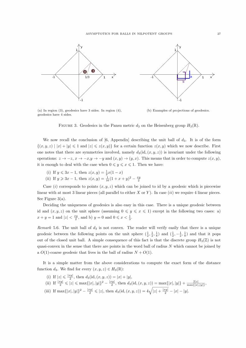
ASYMPTOTICS FOR BALLS IN NILPOTENT GROUPS 27
(a) In region (3), geodesics have 3 sides. In region (4),geodesics have 4 sides.
(b) Examples of projections of geodesics.
Figure 3. Geodesics in the Pansu metric d3 on the Heisenberg group H3(R).
We now recall the conclusion of [6, Appendix] describing the unit ball of d3. It is of the form
(x, y, z) | |x| + |y| 6 1 and |z| 6 z(x, y) for a certain function z(x, y) which we now describe. First
one notes that there are symmetries involved, namely d3(id, (x, y, z)) is invariant under the following
operations: z → −z, x→ −x,y → −y and (x, y) → (y, x). This means that in order to compute z(x, y),
it is enough to deal with the case when 0 6 y 6 x 6 1. Then we have:
(i) If y 6 3x− 1, then z(x, y) = 12x(1− x)
(ii) If y > 3x− 1, then z(x, y) = 116 (1 + x+ y)2 − xy
2
Case (i) corresponds to points (x, y, z) which can be joined to id by a geodesic which is piecewise
linear with at most 3 linear pieces (all parallel to either X or Y ). In case (ii) we require 4 linear pieces.
See Figure 3(a).
Deciding the uniqueness of geodesics is also easy in this case. There is a unique geodesic between
id and (x, y, z) on the unit sphere (assuming 0 6 y 6 x 6 1) except in the following two cases: a)
x+ y = 1 and |z| < xy2 , and b) y = 0 and 0 6 x < 1
3 .
Remark 5.6. The unit ball of d3 is not convex. The reader will verify easily that there is a unique
geodesic between the following points on the unit sphere ( 12 ,12 ,
18 ) and ( 12 ,−
12 ,
18 ) and that it pops
out of the closed unit ball. A simple consequence of this fact is that the discrete group H3(Z) is not
quasi-convex in the sense that there are points in the word ball of radius N which cannot be joined by
a O(1)-coarse geodesic that lives in the ball of radius N +O(1).
It is a simple matter from the above considerations to compute the exact form of the distance
function d3. We find for every (x, y, z) ∈ H3(R):
(i) If |z| 6 |xy|2 , then d3(id, (x, y, z)) = |x|+ |y|,
(ii) If |xy|2 6 |z| 6 max|x|, |y|2 − |xy|
2 , then d3(id, (x, y, z)) = max|x|, |y|+ 2|z|max|x|,|y| ,
(iii) If max|x|, |y|2 − |xy|2 6 |z|, then d3(id, (x, y, z)) = 4
√|z|+ |xy|
2 − |x| − |y|.
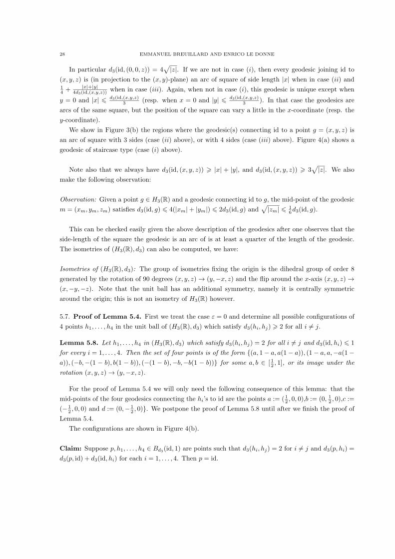
28 EMMANUEL BREUILLARD AND ENRICO LE DONNE
In particular d3(id, (0, 0, z)) = 4√|z|. If we are not in case (i), then every geodesic joining id to
(x, y, z) is (in projection to the (x, y)-plane) an arc of square of side length |x| when in case (ii) and14 + |x|+|y|
4d3(id,(x,y,z))when in case (iii). Again, when not in case (i), this geodesic is unique except when
y = 0 and |x| 6 d3(id,(x,y,z)3 (resp. when x = 0 and |y| 6 d3(id,(x,y,z)
3 ). In that case the geodesics are
arcs of the same square, but the position of the square can vary a little in the x-coordinate (resp. the
y-coordinate).
We show in Figure 3(b) the regions where the geodesic(s) connecting id to a point g = (x, y, z) is
an arc of square with 3 sides (case (ii) above), or with 4 sides (case (iii) above). Figure 4(a) shows a
geodesic of staircase type (case (i) above).
Note also that we always have d3(id, (x, y, z)) > |x| + |y|, and d3(id, (x, y, z)) > 3√
|z|. We also
make the following observation:
Observation: Given a point g ∈ H3(R) and a geodesic connecting id to g, the mid-point of the geodesic
m = (xm, ym, zm) satisfies d3(id, g) 6 4(|xm|+ |ym|) 6 2d3(id, g) and√|zm| 6 1
6d3(id, g).
This can be checked easily given the above description of the geodesics after one observes that the
side-length of the square the geodesic is an arc of is at least a quarter of the length of the geodesic.
The isometries of (H3(R), d3) can also be computed, we have:
Isometries of (H3(R), d3): The group of isometries fixing the origin is the dihedral group of order 8
generated by the rotation of 90 degrees (x, y, z) → (y,−x, z) and the flip around the x-axis (x, y, z) →(x,−y,−z). Note that the unit ball has an additional symmetry, namely it is centrally symmetric
around the origin; this is not an isometry of H3(R) however.
5.7. Proof of Lemma 5.4. First we treat the case ε = 0 and determine all possible configurations of
4 points h1, . . . , h4 in the unit ball of (H3(R), d3) which satisfy d3(hi, hj) > 2 for all i = j.
Lemma 5.8. Let h1, . . . , h4 in (H3(R), d3) which satisfy d3(hi, hj) = 2 for all i = j and d3(id, hi) 6 1
for every i = 1, . . . , 4. Then the set of four points is of the form (a, 1− a, a(1− a)), (1− a, a,−a(1−a)), (−b,−(1 − b), b(1 − b)), (−(1 − b),−b,−b(1 − b)) for some a, b ∈ [ 12 , 1], or its image under the
rotation (x, y, z) → (y,−x, z).
For the proof of Lemma 5.4 we will only need the following consequence of this lemma: that the
mid-points of the four geodesics connecting the hi’s to id are the points a := ( 12 , 0, 0),b := (0, 12 , 0),c :=
(−12 , 0, 0) and d := (0,−1
2 , 0). We postpone the proof of Lemma 5.8 until after we finish the proof of
Lemma 5.4.
The configurations are shown in Figure 4(b).
Claim: Suppose p, h1, . . . , h4 ∈ Bd3(id, 1) are points such that d3(hi, hj) = 2 for i = j and d3(p, hi) =
d3(p, id) + d3(id, hi) for each i = 1, . . . , 4. Then p = id.
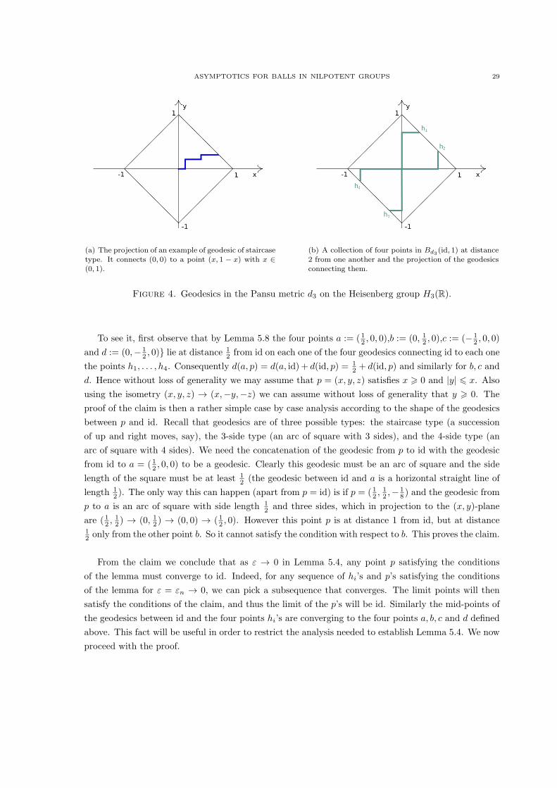
ASYMPTOTICS FOR BALLS IN NILPOTENT GROUPS 29
(a) The projection of an example of geodesic of staircasetype. It connects (0, 0) to a point (x, 1 − x) with x ∈(0, 1).
(b) A collection of four points in Bd3 (id, 1) at distance2 from one another and the projection of the geodesicsconnecting them.
Figure 4. Geodesics in the Pansu metric d3 on the Heisenberg group H3(R).
To see it, first observe that by Lemma 5.8 the four points a := ( 12 , 0, 0),b := (0, 12 , 0),c := (− 12 , 0, 0)
and d := (0,−12 , 0) lie at distance 1
2 from id on each one of the four geodesics connecting id to each one
the points h1, . . . , h4. Consequently d(a, p) = d(a, id) + d(id, p) = 12 + d(id, p) and similarly for b, c and
d. Hence without loss of generality we may assume that p = (x, y, z) satisfies x > 0 and |y| 6 x. Also
using the isometry (x, y, z) → (x,−y,−z) we can assume without loss of generality that y > 0. The
proof of the claim is then a rather simple case by case analysis according to the shape of the geodesics
between p and id. Recall that geodesics are of three possible types: the staircase type (a succession
of up and right moves, say), the 3-side type (an arc of square with 3 sides), and the 4-side type (an
arc of square with 4 sides). We need the concatenation of the geodesic from p to id with the geodesic
from id to a = ( 12 , 0, 0) to be a geodesic. Clearly this geodesic must be an arc of square and the side
length of the square must be at least 12 (the geodesic between id and a is a horizontal straight line of
length 12 ). The only way this can happen (apart from p = id) is if p = ( 12 ,
12 ,−
18 ) and the geodesic from
p to a is an arc of square with side length 12 and three sides, which in projection to the (x, y)-plane
are ( 12 ,12 ) → (0, 12 ) → (0, 0) → ( 12 , 0). However this point p is at distance 1 from id, but at distance
12 only from the other point b. So it cannot satisfy the condition with respect to b. This proves the claim.
From the claim we conclude that as ε → 0 in Lemma 5.4, any point p satisfying the conditions
of the lemma must converge to id. Indeed, for any sequence of hi’s and p’s satisfying the conditions
of the lemma for ε = εn → 0, we can pick a subsequence that converges. The limit points will then
satisfy the conditions of the claim, and thus the limit of the p’s will be id. Similarly the mid-points of
the geodesics between id and the four points hi’s are converging to the four points a, b, c and d defined
above. This fact will be useful in order to restrict the analysis needed to establish Lemma 5.4. We now
proceed with the proof.
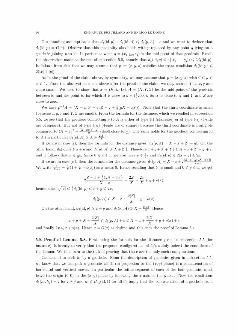
30 EMMANUEL BREUILLARD AND ENRICO LE DONNE
Our standing assumption is that d3(id, p) + d3(id, A) 6 d3(p,A) + ε and we want to deduce that
d3(id, p) = O(ε). Observe that this inequality also holds with p replaced by any point q lying on a
geodesic joining p to id. In particular when q = (xq, yq, zq) is the mid-point of that geodesic. Recall
the observation made at the end of subsection 5.5, namely that d3(id, p) 6 4(|xq| + |yq|) 6 2d3(id, p).
It follows from this that we may assume that p := (x, y, z) satisfies the extra condition d3(id, p) 62(|x|+ |y|).
As in the proof of the claim above, by symmetry, we may assume that p = (x, y, z) with 0 6 y 6x 6 1. From the observation made above after the proof of the claim, we may assume that x, y and
z are small. We need to show that x = O(ε). Let A = (X,Y, Z) be the mid-point of the geodesic
between id and the point hi for which A is close to a = ( 12 , 0, 0). So X is close to 12 and Y and Z are
close to zero.
We have p−1A = (X − x, Y − y, Z − z + 12 (yX − xY )). Note that the third coordinate is small
(because x, y, z and Y, Z are small). From the formula for the distance, which we recalled in subsection
5.5, we see that the geodesic connecting p to A is either of type (i) (staircase) or of type (ii) (3-side
arc of square). But not of type (iii) (4-side arc of square) because the third coordinate is negligible
compared to (X − x)2 − (X−x)(Y−y)2 (itself close to 1
4 ). The same holds for the geodesic connecting id
to A (in particular d3(id, A) > X + 2|Z|X ).
If we are in case (i), then the formula for the distance gives: d3(p,A) = X − x + |Y − y|. On the
other hand, d3(id, p) > x+ y and d3(id, A) > X+ |Y |. Therefore x+ y+X+ |Y | 6 X−x+ |Y − y|+ ε,and it follows that x 6 1
2ε. Since 0 6 y 6 x, we also have y 6 12ε and d3(id, p) 6 2(x+ y) 6 2ε.
If we are in case (ii), then the formula for the distance gives: d3(p,A) = X −x+2|Z−z+ 1
2 (yX−xY )|X−x .
We write 1X−x = 1
X (1 + xX + o(x)) as x nears 0. Hence recalling that Y is small and 0 6 y 6 x, we get
2Z − z + 1
2 (yX − xY )
X − x=
2Z
X− 2z
X+ y + o(x),
hence, since√|z| 6 1
3d3(id, p) 6 x+ y 6 2x,
d3(p,A) 6 X − x+2|Z|X
+ y + o(x).
On the other hand, d3(id, p) > x+ y and d3(id, A) > X + 2|Z|X . Hence
x+ y +X +2|Z|X
6 d3(p,A) + ε 6 X − x+2|Z|X
+ y + o(x) + ε
and finally 2x 6 ε+ o(x). Hence x = O(ε) as desired and this ends the proof of Lemma 5.4.
5.9. Proof of Lemma 5.8. First, using the formula for the distance given in subsection 5.5 (for
instance), it is easy to verify that the proposed configurations of hi’s satisfy indeed the conditions of
the lemma. We thus turn to the task of proving that these are the only such configurations.
Connect id to each hi by a geodesic. From the description of geodesics given in subsection 5.5,
we know that we can pick a geodesic which (in projection to the (x, y)-plane) is a concatenation of
horizontal and vertical moves. In particular the initial segment of each of the four geodesics must
leave the origin (0, 0) in the (x, y)-plane by following the x-axis or the y-axis. Now the conditions
d3(hi, hj) = 2 for i = j and hi ∈ Bd3(id, 1) for all i’s imply that the concatenation of a geodesic from
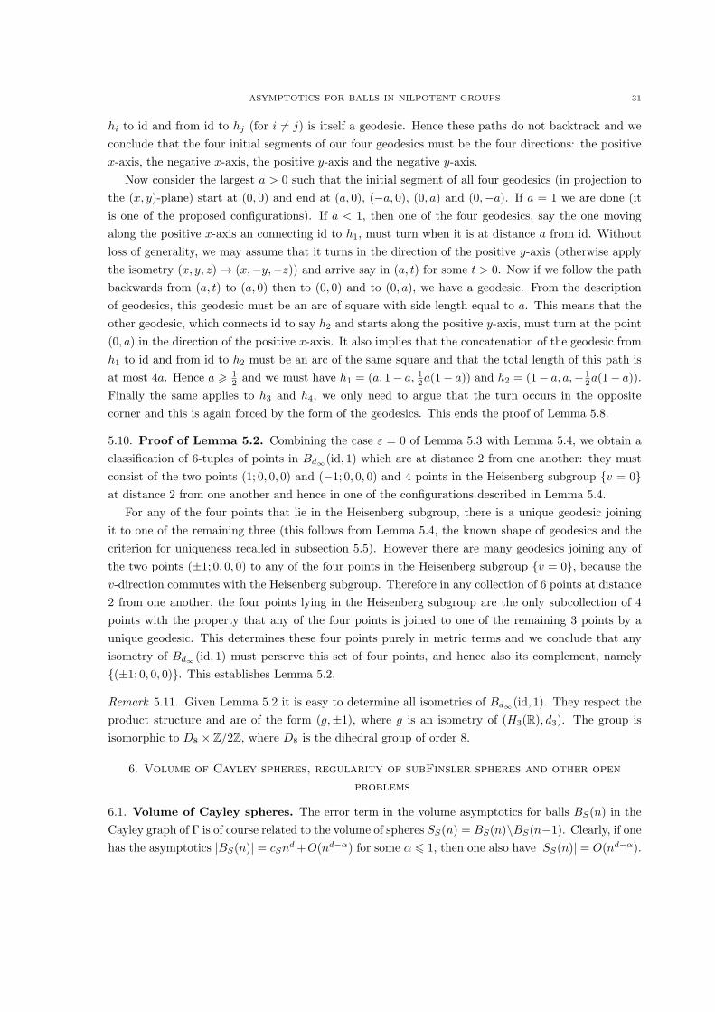
ASYMPTOTICS FOR BALLS IN NILPOTENT GROUPS 31
hi to id and from id to hj (for i = j) is itself a geodesic. Hence these paths do not backtrack and we
conclude that the four initial segments of our four geodesics must be the four directions: the positive
x-axis, the negative x-axis, the positive y-axis and the negative y-axis.
Now consider the largest a > 0 such that the initial segment of all four geodesics (in projection to
the (x, y)-plane) start at (0, 0) and end at (a, 0), (−a, 0), (0, a) and (0,−a). If a = 1 we are done (it
is one of the proposed configurations). If a < 1, then one of the four geodesics, say the one moving
along the positive x-axis an connecting id to h1, must turn when it is at distance a from id. Without
loss of generality, we may assume that it turns in the direction of the positive y-axis (otherwise apply
the isometry (x, y, z) → (x,−y,−z)) and arrive say in (a, t) for some t > 0. Now if we follow the path
backwards from (a, t) to (a, 0) then to (0, 0) and to (0, a), we have a geodesic. From the description
of geodesics, this geodesic must be an arc of square with side length equal to a. This means that the
other geodesic, which connects id to say h2 and starts along the positive y-axis, must turn at the point
(0, a) in the direction of the positive x-axis. It also implies that the concatenation of the geodesic from
h1 to id and from id to h2 must be an arc of the same square and that the total length of this path is
at most 4a. Hence a > 12 and we must have h1 = (a, 1− a, 12a(1− a)) and h2 = (1− a, a,−1
2a(1− a)).
Finally the same applies to h3 and h4, we only need to argue that the turn occurs in the opposite
corner and this is again forced by the form of the geodesics. This ends the proof of Lemma 5.8.
5.10. Proof of Lemma 5.2. Combining the case ε = 0 of Lemma 5.3 with Lemma 5.4, we obtain a
classification of 6-tuples of points in Bd∞(id, 1) which are at distance 2 from one another: they must
consist of the two points (1; 0, 0, 0) and (−1; 0, 0, 0) and 4 points in the Heisenberg subgroup v = 0at distance 2 from one another and hence in one of the configurations described in Lemma 5.4.
For any of the four points that lie in the Heisenberg subgroup, there is a unique geodesic joining
it to one of the remaining three (this follows from Lemma 5.4, the known shape of geodesics and the
criterion for uniqueness recalled in subsection 5.5). However there are many geodesics joining any of
the two points (±1; 0, 0, 0) to any of the four points in the Heisenberg subgroup v = 0, because the
v-direction commutes with the Heisenberg subgroup. Therefore in any collection of 6 points at distance
2 from one another, the four points lying in the Heisenberg subgroup are the only subcollection of 4
points with the property that any of the four points is joined to one of the remaining 3 points by a
unique geodesic. This determines these four points purely in metric terms and we conclude that any
isometry of Bd∞(id, 1) must perserve this set of four points, and hence also its complement, namely
(±1; 0, 0, 0). This establishes Lemma 5.2.
Remark 5.11. Given Lemma 5.2 it is easy to determine all isometries of Bd∞(id, 1). They respect the
product structure and are of the form (g,±1), where g is an isometry of (H3(R), d3). The group is
isomorphic to D8 × Z/2Z, where D8 is the dihedral group of order 8.
6. Volume of Cayley spheres, regularity of subFinsler spheres and other open
problems
6.1. Volume of Cayley spheres. The error term in the volume asymptotics for balls BS(n) in the
Cayley graph of Γ is of course related to the volume of spheres SS(n) = BS(n)\BS(n−1). Clearly, if one
has the asymptotics |BS(n)| = cSnd+O(nd−α) for some α 6 1, then one also have |SS(n)| = O(nd−α).
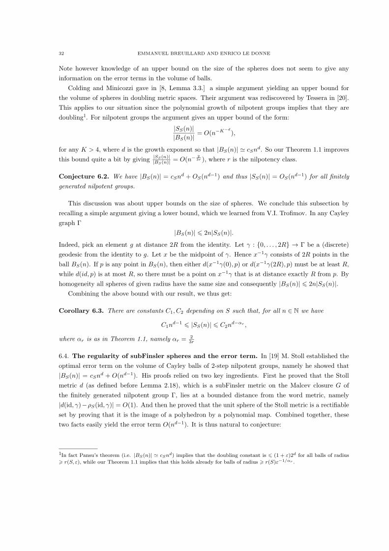
32 EMMANUEL BREUILLARD AND ENRICO LE DONNE
Note however knowledge of an upper bound on the size of the spheres does not seem to give any
information on the error terms in the volume of balls.
Colding and Minicozzi gave in [8, Lemma 3.3.] a simple argument yielding an upper bound for
the volume of spheres in doubling metric spaces. Their argument was rediscovered by Tessera in [20].
This applies to our situation since the polynomial growth of nilpotent groups implies that they are
doubling1. For nilpotent groups the argument gives an upper bound of the form:
|SS(n)||BS(n)|
= O(n−K−d
),
for any K > 4, where d is the growth exponent so that |BS(n)| ≃ cSnd. So our Theorem 1.1 improves
this bound quite a bit by giving |SS(n)||BS(n)| = O(n−
23r ), where r is the nilpotency class.
Conjecture 6.2. We have |BS(n)| = cSnd + OS(n
d−1) and thus |SS(n)| = OS(nd−1) for all finitely
generated nilpotent groups.
This discussion was about upper bounds on the size of spheres. We conclude this subsection by
recalling a simple argument giving a lower bound, which we learned from V.I. Trofimov. In any Cayley
graph Γ
|BS(n)| 6 2n|SS(n)|.
Indeed, pick an element g at distance 2R from the identity. Let γ : 0, . . . , 2R → Γ be a (discrete)
geodesic from the identity to g. Let x be the midpoint of γ. Hence x−1γ consists of 2R points in the
ball BS(n). If p is any point in BS(n), then either d(x−1γ(0), p) or d(x−1γ(2R), p) must be at least R,
while d(id, p) is at most R, so there must be a point on x−1γ that is at distance exactly R from p. By
homogeneity all spheres of given radius have the same size and consequently |BS(n)| 6 2n|SS(n)|.Combining the above bound with our result, we thus get:
Corollary 6.3. There are constants C1, C2 depending on S such that, for all n ∈ N we have
C1nd−1 6 |SS(n)| 6 C2n
d−αr ,
where αr is as in Theorem 1.1, namely αr = 23r
6.4. The regularity of subFinsler spheres and the error term. In [19] M. Stoll established the
optimal error term on the volume of Cayley balls of 2-step nilpotent groups, namely he showed that
|BS(n)| = cSnd + O(nd−1). His proofs relied on two key ingredients. First he proved that the Stoll
metric d (as defined before Lemma 2.18), which is a subFinsler metric on the Malcev closure G of
the finitely generated nilpotent group Γ, lies at a bounded distance from the word metric, namely
|d(id, γ)−ρS(id, γ)| = O(1). And then he proved that the unit sphere of the Stoll metric is a rectifiable
set by proving that it is the image of a polyhedron by a polynomial map. Combined together, these
two facts easily yield the error term O(nd−1). It is thus natural to conjecture:
1In fact Pansu’s theorem (i.e. |BS(n)| ≃ cSnd) implies that the doubling constant is 6 (1 + ε)2d for all balls of radius
> r(S, ε), while our Theorem 1.1 implies that this holds already for balls of radius > r(S)ε−1/αr .
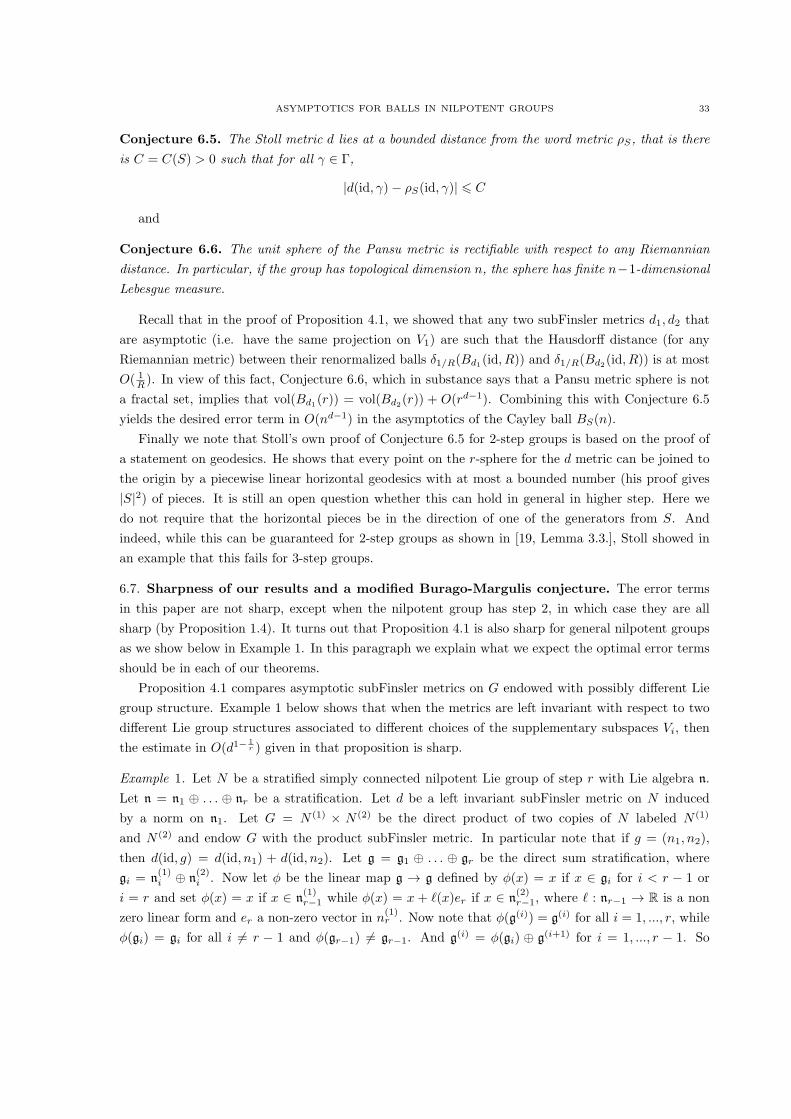
ASYMPTOTICS FOR BALLS IN NILPOTENT GROUPS 33
Conjecture 6.5. The Stoll metric d lies at a bounded distance from the word metric ρS, that is there
is C = C(S) > 0 such that for all γ ∈ Γ,
|d(id, γ)− ρS(id, γ)| 6 C
and
Conjecture 6.6. The unit sphere of the Pansu metric is rectifiable with respect to any Riemannian
distance. In particular, if the group has topological dimension n, the sphere has finite n−1-dimensional
Lebesgue measure.
Recall that in the proof of Proposition 4.1, we showed that any two subFinsler metrics d1, d2 that
are asymptotic (i.e. have the same projection on V1) are such that the Hausdorff distance (for any
Riemannian metric) between their renormalized balls δ1/R(Bd1(id, R)) and δ1/R(Bd2(id, R)) is at most
O( 1R ). In view of this fact, Conjecture 6.6, which in substance says that a Pansu metric sphere is not
a fractal set, implies that vol(Bd1(r)) = vol(Bd2(r)) + O(rd−1). Combining this with Conjecture 6.5
yields the desired error term in O(nd−1) in the asymptotics of the Cayley ball BS(n).
Finally we note that Stoll’s own proof of Conjecture 6.5 for 2-step groups is based on the proof of
a statement on geodesics. He shows that every point on the r-sphere for the d metric can be joined to
the origin by a piecewise linear horizontal geodesics with at most a bounded number (his proof gives
|S|2) of pieces. It is still an open question whether this can hold in general in higher step. Here we
do not require that the horizontal pieces be in the direction of one of the generators from S. And
indeed, while this can be guaranteed for 2-step groups as shown in [19, Lemma 3.3.], Stoll showed in
an example that this fails for 3-step groups.
6.7. Sharpness of our results and a modified Burago-Margulis conjecture. The error terms
in this paper are not sharp, except when the nilpotent group has step 2, in which case they are all
sharp (by Proposition 1.4). It turns out that Proposition 4.1 is also sharp for general nilpotent groups
as we show below in Example 1. In this paragraph we explain what we expect the optimal error terms
should be in each of our theorems.
Proposition 4.1 compares asymptotic subFinsler metrics on G endowed with possibly different Lie
group structure. Example 1 below shows that when the metrics are left invariant with respect to two
different Lie group structures associated to different choices of the supplementary subspaces Vi, then
the estimate in O(d1−1r ) given in that proposition is sharp.
Example 1. Let N be a stratified simply connected nilpotent Lie group of step r with Lie algebra n.
Let n = n1 ⊕ . . . ⊕ nr be a stratification. Let d be a left invariant subFinsler metric on N induced
by a norm on n1. Let G = N (1) × N (2) be the direct product of two copies of N labeled N (1)
and N (2) and endow G with the product subFinsler metric. In particular note that if g = (n1, n2),
then d(id, g) = d(id, n1) + d(id, n2). Let g = g1 ⊕ . . . ⊕ gr be the direct sum stratification, where
gi = n(1)i ⊕ n
(2)i . Now let ϕ be the linear map g → g defined by ϕ(x) = x if x ∈ gi for i < r − 1 or
i = r and set ϕ(x) = x if x ∈ n(1)r−1 while ϕ(x) = x + ℓ(x)er if x ∈ n
(2)r−1, where ℓ : nr−1 → R is a non
zero linear form and er a non-zero vector in n(1)r . Now note that ϕ(g(i)) = g(i) for all i = 1, ..., r, while
ϕ(gi) = gi for all i = r − 1 and ϕ(gr−1) = gr−1. And g(i) = ϕ(gi) ⊕ g(i+1) for i = 1, ..., r − 1. So
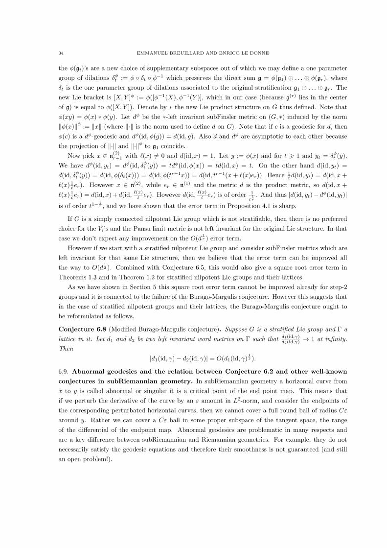
34 EMMANUEL BREUILLARD AND ENRICO LE DONNE
the ϕ(gi)’s are a new choice of supplementary subspaces out of which we may define a one parameter
group of dilations δϕt := ϕ δt ϕ−1 which preserves the direct sum g = ϕ(g1) ⊕ . . . ⊕ ϕ(gr), where
δt is the one parameter group of dilations associated to the original stratification g1 ⊕ . . . ⊕ gr. The
new Lie bracket is [X,Y ]ϕ := ϕ([ϕ−1(X), ϕ−1(Y )], which in our case (because g(r) lies in the center
of g) is equal to ϕ([X,Y ]). Denote by ∗ the new Lie product structure on G thus defined. Note that
ϕ(xy) = ϕ(x) ∗ ϕ(y). Let dϕ be the ∗-left invariant subFinsler metric on (G, ∗) induced by the norm
∥ϕ(x)∥ϕ := ∥x∥ (where ∥·∥ is the norm used to define d on G). Note that if c is a geodesic for d, then
ϕ(c) is a dϕ-geodesic and dϕ(id, ϕ(g)) = d(id, g). Also d and dϕ are asymptotic to each other because
the projection of ∥·∥ and ∥·∥ϕ to g1 coincide.
Now pick x ∈ n(2)r−1 with ℓ(x) = 0 and d(id, x) = 1. Let y := ϕ(x) and for t > 1 and yt = δϕt (y).
We have dϕ(id, yt) = dϕ(id, δϕt (y)) = tdϕ(id, ϕ(x)) = td(id, x) = t. On the other hand d(id, yt) =
d(id, δϕt (y)) = d(id, ϕ(δt(x))) = d(id, ϕ(tr−1x)) = d(id, tr−1(x + ℓ(x)er)). Hence 1t d(id, yt) = d(id, x +
ℓ(x) 1t er). However x ∈ n(2), while er ∈ n(1) and the metric d is the product metric, so d(id, x +
ℓ(x) 1t er) = d(id, x)+ d(id, ℓ(x)t er). However d(id,ℓ(x)t er) is of order
1
t1r. And thus |d(id, yt)− dϕ(id, yt)|
is of order t1−1r , and we have shown that the error term in Proposition 4.1 is sharp.
If G is a simply connected nilpotent Lie group which is not stratifiable, then there is no preferred
choice for the Vi’s and the Pansu limit metric is not left invariant for the original Lie structure. In that
case we don’t expect any improvement on the O(d1r ) error term.
However if we start with a stratified nilpotent Lie group and consider subFinsler metrics which are
left invariant for that same Lie structure, then we believe that the error term can be improved all
the way to O(d12 ). Combined with Conjecture 6.5, this would also give a square root error term in
Theorems 1.3 and in Theorem 1.2 for stratified nilpotent Lie groups and their lattices.
As we have shown in Section 5 this square root error term cannot be improved already for step-2
groups and it is connected to the failure of the Burago-Margulis conjecture. However this suggests that
in the case of stratified nilpotent groups and their lattices, the Burago-Margulis conjecture ought to
be reformulated as follows.
Conjecture 6.8 (Modified Burago-Margulis conjecture). Suppose G is a stratified Lie group and Γ a
lattice in it. Let d1 and d2 be two left invariant word metrics on Γ such that d1(id,γ)d2(id,γ)
→ 1 at infinity.
Then
|d1(id, γ)− d2(id, γ)| = O(d1(id, γ)12 ).
6.9. Abnormal geodesics and the relation between Conjecture 6.2 and other well-known
conjectures in subRiemannian geometry. In subRiemannian geometry a horizontal curve from
x to y is called abnormal or singular it is a critical point of the end point map. This means that
if we perturb the derivative of the curve by an ε amount in L2-norm, and consider the endpoints of
the corresponding perturbated horizontal curves, then we cannot cover a full round ball of radius Cε
around y. Rather we can cover a Cε ball in some proper subspace of the tangent space, the range
of the differential of the endpoint map. Abnormal geodesics are problematic in many respects and
are a key difference between subRiemannian and Riemannian geometries. For example, they do not
necessarily satisfy the geodesic equations and therefore their smoothness is not guaranteed (and still
an open problem!).
ASYMPTOTICS FOR BALLS IN NILPOTENT GROUPS 35
Abnormal geodesics exist in most Carnot groups. For example, pieces of horizontal one-parameter
subgroups are abnormal geodesics in the free nilpotent Lie group of rank at least 3 (in every step > 2).
In the Heisenberg groups however, there are no abnormal geodesics.
It turns out that the presence of abnormal geodesics is precisely the reason why the Burago-Margulis
fails. The counter-example from [6, §8.2] and Section 5 of the present paper are based on the idea that
given two asymptotic metrics, an abnormal curve can be a geodesic for one metric, but be far from
being a geodesic for the other. The absence of abnormal geodesics in the Heisenberg group is precisely
what is responsible for the fact that asymptotic left invariant metrics are always at a bounded distance
from each other on this group (Krat’s theorem [13]). However this is an exceptional case. One can
see the absence of abnormal geodesics in the Heisenberg group by looking at Figure 1 and noting that
the sphere has no cusps (near every point, the sphere looks like a standard full dimensional cone).
In the counter-example to the Burago-Margulis conjecture however (see Figure 5), the presence of
the abnormal curve (in red in the picture) produces a cusp on the unit sphere (the z-direction gets
squashed).
Abnormal geodesics are also behind Conjecture 6.6 above, in fact they are the reason why this
conjecture is not obvious and hence neither is the O(rd−1) error term in the volume asymptotics
of r-balls for subFinsler metrics. Indeed if there were no abnormal geodesic, the distance function
g 7→ d(id, g) would be smooth and its level sets (the spheres) would be rectifiable. Note that it is
known that for certain Carnot-Caratheodory manifolds, the distance function and the spheres are not
subanalytic (see [5]).
Even if abnormal curves exist in most Carnot groups, they are conjectured to be sparse. According
to Montgomery [16, chapter 10.2] there ought to be a Sard theorem for the endpoint map, implying in
particular that the set of points in G which can be reached by a singular curve of length at most 1,
say, must be a nowhere dense set of zero Lebesgue measure. This is still an open problem for general
Carnot groups. Should the answer be yes, it would then be possible to prove that subFinsler spheres
are not fractal objects and that the d− 1-dimensional Lebesgue measure of subFinsler spheres is finite.
This would be enough to establish the O(rd−1) error term in the volume asymptotics of left invariant
subFinsler metrics on Carnot groups.
References
[1] Geometric group theory, hyperbolic dynamics and symplectic geometry. Oberwolfach Rep., 3(3):1991–2057, 2006.
Abstracts from the workshop held July 23–29, 2006, Organized by Gerhard Knieper, Leonid Polterovich and Leonid
Potyagailo, Oberwolfach Reports. Vol. 3, no. 3.
[2] H. Abels and G. Margulis. Coarsely geodesic metrics on reductive groups. In Modern dynamical systems and appli-
cations, pages 163–183. Cambridge Univ. Press, Cambridge, 2004.
[3] H. Bass. The degree of polynomial growth of finitely generated nilpotent groups. Proc. London Math. Soc. (3),
25:603–614, 1972.
[4] V. N. Berestovskiı. Homogeneous manifolds with an intrinsic metric. I. Sibirsk. Mat. Zh., 29(6):17–29, 1988.
[5] B. Bonnard, M. Chyba, and I. Kupka. Nonintegrable geodesics in SR-Martinet geometry. In Differential geometry
and control (Boulder, CO, 1997), volume 64 of Proc. Sympos. Pure Math., pages 119–134. Amer. Math. Soc.,
Providence, RI, 1999.
[6] E. Breuillard. Geometry of groups of polynomial growth and shape of large balls. arXiv:0704.0095, 2007. Preprint.
36 EMMANUEL BREUILLARD AND ENRICO LE DONNE
[7] D. Y. Burago. Periodic metrics. In Representation theory and dynamical systems, volume 9 of Adv. Soviet Math.,
pages 205–210. Amer. Math. Soc., Providence, RI, 1992.
[8] T. H. Colding and W. P. Minicozzi, II. Liouville theorems for harmonic sections and applications. Comm. Pure
Appl. Math., 51(2):113–138, 1998.
[9] M. Duchin, S. Lelievre, and C. Mooney. The geometry of spheres in free abelian groups. arXiv:1004.0053, 2009.
Preprint.
[10] M. Gromov. Groups of polynomial growth and expanding maps. Inst. Hautes Etudes Sci. Publ. Math., (53):53–73,
1981.
[11] M. Gromov. Metric structures for Riemannian and non-Riemannian spaces, volume 152 of Progress in Mathematics.
Birkhauser Boston Inc., Boston, MA, 1999. Based on the 1981 French original, With appendices by M. Katz, P.
Pansu and S. Semmes, Translated from the French by Sean Michael Bates.
[12] Y. Guivarc’h. Croissance polynomiale et periodes des fonctions harmoniques. Bull. Soc. Math. France, 101:333–379,
1973.
[13] S. A. Krat. Asymptotic properties of the Heisenberg group. Zap. Nauchn. Sem. S.-Peterburg. Otdel. Mat. Inst.
Steklov. (POMI), 261(Geom. i Topol. 4):125–154, 268, 1999.
[14] E. Le Donne. Lecture notes on sub-Riemannian geometry. Preprint, 2010.
[15] E. Le Donne. Geodesic manifolds with a transitive subset of smooth biLipschitz maps. Groups Geom. Dyn., 5(3):567–
602, 2011.
[16] R. Montgomery. A tour of subriemannian geometries, their geodesics and applications, volume 91 of Mathematical
Surveys and Monographs. American Mathematical Society, Providence, RI, 2002.
[17] P. Pansu. Croissance des boules et des geodesiques fermees dans les nilvarietes. Ergodic Theory Dynam. Systems,
3(3):415–445, 1983.
[18] M. S. Raghunathan. Discrete subgroups of Lie groups. Springer-Verlag, New York, 1972. Ergebnisse der Mathematik
und ihrer Grenzgebiete, Band 68.
[19] M. Stoll. On the asymptotics of the growth of 2-step nilpotent groups. J. London Math. Soc. (2), 58(1):38–48, 1998.
[20] R. Tessera. Volume of spheres in doubling metric measured spaces and in groups of polynomial growth. Bull. Soc.
Math. France, 135(1):47–64, 2007.
[21] L. van den Dries and A. J. Wilkie. Gromov’s theorem on groups of polynomial growth and elementary logic. J.
Algebra, 89(2):349–374, 1984.
[22] J. A. Wolf. Growth of finitely generated solvable groups and curvature of Riemanniann manifolds. J. Differential
Geometry, 2:421–446, 1968.
Laboratoire de Mathematiques, Batiment 425, Universite Paris Sud 11, 91405 Orsay, FRANCE
E-mail address: [email protected]
Laboratoire de Mathematiques, Batiment 425, Universite Paris Sud 11, 91405 Orsay, FRANCE
E-mail address: [email protected], [email protected]