On the Asymptotic Expansion of the Spheroidal Wave ...barrowes/papers/barrowes_siam2003.pdf ·...

On the Asymptotic Expansion of the

Spheroidal Wave Function and its Eigenvalues

for Complex Size Parameter

Benjamin E. Barrowes, Kevin O’Neill, Tomasz M. Grzegorczyk and Jin A. Kong

Abstract

We provide a rapid and accurate method for calculating the prolate and oblate spheroidal wave

functions (PSWFs and OSWFs), Smn(c, η), and their eigenvalues, λmn, for arbitrary complex size

parameter c in the asymptotic regime of large |c|, m and n fixed. The ability to calculate these SWFs for

large and complex size parameters is important for many applications in mathematics, engineering, and

physics. For arbitrary arg(c), the PSWFs and their eigenvalues are accurately expressed by established

prolate-type or oblate-type asymptotic expansions. However, determining the proper expansion type is

dependent upon finding spheroidal branch points, cmn◦;r , in the complex c-plane where the PSWF alternates

expansion type due to analytic continuation. We implement a numerical search method for tabulating

these branch points as a function of spheroidal parameters m, n, and arg(c). The resulting table allows

rapid determination of the appropriate asymptotic expansion type of the SWFs. Normalizations, which

are dependent on c, are derived for both the prolate and oblate-type asymptotic expansions and for both

(n − m) even and odd. The ordering for these expansions is different from the original ordering of

the SWFs and is dictated by the location of cmn◦;r . We document this ordering for the specific case of

arg(c) = π/4 which occurs for the diffusion equation in spheroidal coordinates. Some representative

values of λmn and Smn(c, η) for large, complex c are also given.

Benjamin E. Barrowes, Tomasz M. Grzegorczyk, and Jin A. Kong are with the Research Laboratory of Electronics and

Department of Electrical Engineering and Computer Science, Massachusetts Institute of Technology, Cambridge, MA 02139-

4307

Kevin O’Neill is with the Cold Regions Research and Engineering Laboratory, 72 Lyme Road, Hanover, New Hampshire,

USA 03755-1290

This work was supported by the Strategic Environmental Research and Development Program and the United Stated Army

Corps of Engineers ERDC UXO EQT program.

October 20, 2003 DRAFT

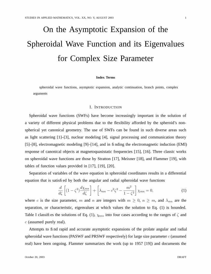
STUDIES IN APPLIED MATHEMATICS, VOL. XX, NO. Y, AUGUST 2003 1

On the Asymptotic Expansion of the

Spheroidal Wave Function and its Eigenvalues

for Complex Size Parameter

Index Terms

spheroidal wave functions, asymptotic expansion, analytic continuation, branch points, complex

arguments

I. INTRODUCTION

Spheroidal wave functions (SWFs) have become increasingly important in the solution of

a variety of different physical problems due to the flexibility afforded by the spheroid’s non-

spherical yet canonical geometry. The use of SWFs can be found in such diverse areas such

as light scattering [1]–[3], nuclear modeling [4], signal processing and communication theory

[5]–[8], electromagnetic modeling [9]–[14], and in finding the electromagnetic induction (EMI)

response of canonical objects at magnetoquasistatic frequencies [15], [16]. Three classic works

on spheroidal wave functions are those by Stratton [17], Meixner [18], and Flammer [19], with

tables of function values provided in [17], [19], [20].

Separation of variables of the wave equation in spheroidal coordinates results in a differential

equation that is satisfied by both the angular and radial spheroidal wave functions

d

dζ

[

(1 − ζ2)dχmn

dζ

]

+

[

λmn − c2ζ2 − m2

1 − ζ2

]

χmn = 0, (1)

where c is the size parameter, m and n are integers with m ≥ 0, n ≥ m, and λmn are the

separation, or characteristic, eigenvalues at which values the solution to Eq. (1) is bounded.

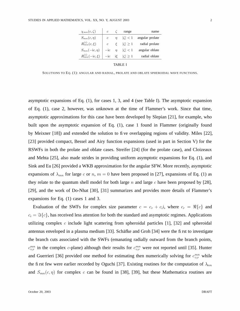
Table I classifies the solutions of Eq. (1), χmn, into four cases according to the ranges of ζ and

c (assumed purely real).

Attempts to find rapid and accurate asymptotic expansions of the prolate angular and radial

spheroidal wave functions (PASWF and PRSWF respectively) for large size parameter c (assumed

real) have been ongoing. Flammer summarizes the work (up to 1957 [19]) and documents the



χmn(c, ζ) c ζ range name

Smn(c, η) c η |ζ| < 1 angular prolate

R(i)mn(c, ξ) c ξ |ζ| ≥ 1 radial prolate

Smn(−ic, η) −ic η |ζ| < 1 angular oblate

R(i)mn(−ic, ξ) −ic iξ |ζ| ≥ 1 radial oblate

TABLE I

SOLUTIONS TO EQ. (1): ANGULAR AND RADIAL, PROLATE AND OBLATE SPHEROIDAL WAVE FUNCTIONS.

asymptotic expansions of Eq. (1), for cases 1, 3, and 4 (see Table I). The asymptotic expansion

of Eq. (1), case 2, however, was unknown at the time of Flammer’s work. Since that time,

asymptotic approximations for this case have been developed by Slepian [21], for example, who

built upon the asymptotic expansion of Eq. (1), case 1 found in Flammer (originally found

by Meixner [18]) and extended the solution to five overlapping regions of validity. Miles [22],

[23] provided compact, Bessel and Airy function expansions (used in part in Section V) for the

RSWFs in both the prolate and oblate cases. Streifer [24] (for the prolate case), and Cloizeaux

and Mehta [25], also made strides in providing uniform asymptotic expansions for Eq. (1), and

Sink and Eu [26] provided a WKB approximation for the angular SFW. More recently, asymptotic

expansions of λmn for large c or n, m = 0 have been proposed in [27], expansions of Eq. (1) as

they relate to the quantum shell model for both large n and large c have been proposed by [28],

[29], and the work of Do-Nhat [30], [31] summarizes and provides more details of Flammer’s

expansions for Eq. (1) cases 1 and 3.

Evaluation of the SWFs for complex size parameter c = cr + cii, where cr = <{c} and

ci = ={c}, has received less attention for both the standard and asymptotic regimes. Applications

utilizing complex c include light scattering from spheroidal particles [1], [32] and spheroidal

antennas enveloped in a plasma medium [33]. Schafke and Groh [34] were the first to investigate

the branch cuts associated with the SWFs (emanating radially outward from the branch points,

cmn◦;r in the complex c-plane) although their results for cmn

◦;r were not reported until [35]. Hunter

and Guerrieri [36] provided one method for estimating then numerically solving for cmn◦;r while

the first few were earlier recorded by Oguchi [37]. Existing routines for the computation of λmn

and Smn(c, η) for complex c can be found in [38], [39], but these Mathematica routines are



too slow to be used for anything but reference. In addition, it appears that these codes do not

properly determine the expansion type for arg(c) 6= [0, π/4, π/2].

In this paper, we implement a numerical method for first tabulating the branch points cmn◦;r ,

then rapidly and accurately computing the asymptotic expansions of λmn and Smn(c, η) for

arbitrary complex size parameter c in the asymptotic regime of |c| large with n and m fixed.

This regime corresponds to, for example, case (i) in [22] and the regime discussed in part I

of [21]. To accomplish this, the branch points cmn◦;r are incorporated into a lookup table used to

determine which asymptotic expansion is appropriate for a given c. Specifically, we elaborate

on the solution for the specific case of cr = ci, and Table III lists which expansion type applies

for a given m and n under this condition. This special case is encountered in the solution of the

diffusion equation for spheroidal systems [16]. We also provide normalizations for the standard

prolate-type and oblate-type asymptotic expansions for both (n−m) even and odd. Expansions

for the oblate SWFs are also discussed as a simple extension of the current investigation. All

calculations in this paper were performed in double precision except for the Newton-Raphson

method, which was implemented in quadruple precision. The routines presented are rapid enough

to be of practical use in applications requiring the calculation of many SWFs of varying orders,

degrees, and arguments.

The structure of this paper is as follows. Section II reviews the basic geometry and the

definitions of the prolate SWFs. We describe the most common asymptotic expansions of the

spheroidal eigenvalues λmn for purely real or imaginary c in Sections III-A and III-B respectively.

The asymptotic expansion of λmn in the case of complex c depends on finding the branch, or

double, points and our numerical method for finding these points is described in Section III-

C. The ordering of the eigenvalues λmn (and the SWFs) for the case of complex c is not as

straightforward as the case of purely real (PSWFs) or purely imaginary c (Oblate SWFs) but

instead depends on arg(cmn◦;r ) as compared to arg(c). The first few of these branch points are listed

in Table II. Section III-E addresses the expansion ordering and describes how to incorporate this

ordering into existing asymptotic expansions. In Section IV the overall asymptotic expansion of

the PASWF for complex c is shown to be comprised of the established expansions outlined in

Section III, where the choice of which type of asymptotic expansion to use is determined by m, n,

and arg(c) via the same lookup table of branch points used in determining the correct expansion

type for λmn. Proper normalizations for these asymptotic expansions are derived in Section IV-



PSfrag replacements

x

y

z

Ho(r)e−iωt

η

ξφ

dξ = ξo

β interfacea

b

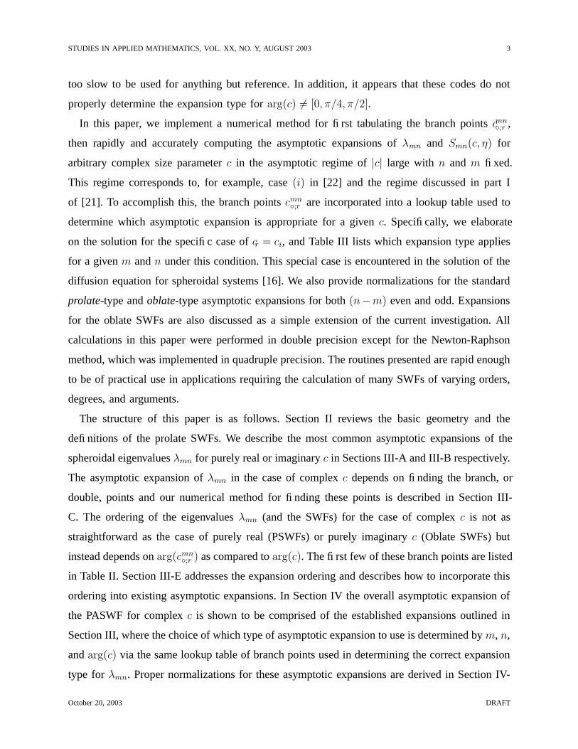
Fig. 1. Prolate Spheroidal Geometry: 1 ≤ ξ < ∞, −1 ≤ η ≤ 1, 0 ≤ φ ≤ 2π, x = d

2[(1 − η2)(ξ2 − 1)]

1

2 cos(φ),

y = d

2[(1 − η2)(ξ2 − 1)]

1

2 sin(φ), z = d

2ηξ, e = b

a, ξ = (1 − e−2)−

1

2 , d = 2(b2 − a2)1

2 .

A. Section V contains a discussion of the expansions and patterns under consideration as well

as some examples in graphical form of the real and imaginary parts of the complex PASWFs,

Smn(c, η) and S ′mn(c, η), as compared to the original Legendre expansion solutions. At the end of

Section V we discuss briefly one asymptotic expansion of the PRSWFs R(i)mn(c, ξ) for complex c,

in light of the current discussion of the PASWFs. This is followed by a conclusion (Section VI)

and information on how to obtain the computer programs implemented for this work.

II. STANDARD FORMULATION OF THE PROLATE ANGULAR SPHEROIDAL WAVE FUNCTION

The prolate and oblate spheroidal coordinate systems are two of the eleven coordinate systems

in which the scalar wave equation

(∇2 + k2)ψ = 0 (2)

is separable. The solution to Eq. (2) in prolate spheroidal coordinates is

ψ(i)pmn = Smn(c, η)R(i)

mn(c, ξ)Tpm(φ), (3)

where c is the size parameter (c = kd/2, where d is the interfocal distance as shown in Fig. 1),

Smn(c, η) is the PASWF, R(i)mn(c, ξ) is a the PRSWF of the ith kind, and Tpm(φ) is the azimuthal



function given by

Tpm(φ) =

cos(mφ), p = 0

sin(mφ), p = 1.(4)

Flammer’s notation [19] is used throughout except for the notation used for the harmonic

functions (Eq. (4)) and some minor notational (but not formal) differences in the asymptotic

expansions of Eqs. (7)-(12) and (13)-(19) below. Expressions such as n = 0(1)6 indicate n

equals [1, . . . , 6] with an increment of 1.

Expressions for the prolate angular and radial functions have been studied for quite some time

beginning with Lame [40] and then Niven [41]. The most common form of the prolate angular

function is expressed as an expansion in terms of associated Legendre functions

Smn(c, η) =

∞∑′

r=0,1

dmnr Pm

m+r(η) (5)

where the prime indicates summation from {01} over {even

odd} indices when (n−m) is {evenodd}. The

radial function can be expressed as an expansion of spherical Bessel functions [42] as

R(i)mn(c, ξ) =

(

ξ2−1ξ2

)m/2

∞∑′

r=0,1

dmnr

(2m+ r)!

r!

∞∑′

r=0,1

dmnr

(2m+ r)!

r!ir+m−nz

(i)m+r(cξ), (6)

where z(i)m+r(cξ) represents the spherical Bessel functions jm+r(cξ), ym+r(cξ), h

(1)m+r(cξ), and

h(2)m+r(cξ), for i = 1, 2, 3, 4 respectively [42]. The expansion coefficients dmn

r are determined

by solving a three term recurrence relation obtained by substituting Eq. (5) into Eq. (1). These

expansions are accurate for small size parameters up to |c| . 30, but encounter numerical

difficulties leading to inaccuracy for larger |c|.

III. ASYMPTOTIC EXPANSION OF THE SPHEROIDAL EIGENVALUES, λmn

Eigenvalues of the spheroidal differential equation, λmn, are special values for which the

equation’s solutions are bounded at ζ = ±1. We first review the two most common asymptotic

expansions of the spheroidal eigenvalues and angular wavefunctions including both the prolate-

type (c purely real) and oblate-type (c purely imaginary) before applying these expansions to

the case of complex size parameter c.

A number of methods can be used to determine the eigenvalues, including the truncation

and solution of the (transcendental) infinite continued fraction equation directly [19], [39];



successive approximations [19]; a power series representation for small |c| [19], [42] followed

by Bouwkamp’s method of refinement [43]; the relaxation method [44], [45]; and an eigenvalue

matrix approach [46] (see also [47], [48]). We prefer to use Hodge’s [46] method because it is

straightforward and rapidly computes the full set of λmn. When c is in the asymptotic regime

considered here, the λmn produced by Hodge’s method require a larger truncation size of the

eigenvalue matrix in order to maintain accuracy, at the cost of increased computation time. In

this case, increased accuracy can be achieved instead by applying either Bouwkamp’s method

or using an asymptotic representation for λmn (see below). It should be noted that Bouwkamp’s

method converges very slowly near the branch points cmn◦;r .

We use the Matlab codes found at [49], modified to accept complex c to calculate the spheroidal

wave functions. These programs are based on those given in [50] and the results for the PSWF

were compared to published tables [17], [19], [20] and found to be in agreement for purely

real and purely imaginary values of small c. Results also matched values for the PSWFs and

eigenvalues for complex c given in [38], [39].

A. Prolate-Type Asymptotic Expansion

The asymptotic expansion typically applied to the PASWF, Smn(c, η), and its characteristic

eigenvalue, λmn, for the case of purely real c (Eq. (1) case 1) consists of an expansion of

Smn(c, η) in terms of a series of parabolic cylinder, or Weber functions [19], [30]. We designate

all asymptotic expansions typically applied to the PSWF for purely real c as prolate-type although

as will be seen in Section III-C, this expansion can also be applied to the OSWF in the case

of arbitrary, complex c. We shall denote the asymptotic expansion by a superscript (a). The

differential equation under these conditions becomes

d

dζ

[

(1 − η2)dSmn

dη

]

+

[

λmn − c2η2 − m2

1 − η2

]

Smn = 0. (7)

If the following substitutions are made:

Smn(c, η) ≈ S(a)mn(c, η) = (1 − η2)

m2 umn(c, η), (8a)

η ⇒ x√2c

(8b)

then in the limit as c↑∞, x fixed, Eq. (7) reduces to

d2umn

dx2+

(

λmn

2c− x2

4

)

= 0 (9)



which is in the form of the parabolic cylinder differential equation. umn(x) is therefore expanded

in terms of an infinite series of parabolic cylinder functions

umn(x) =

∞∑′

r=−∞CrDn−m+r(x) (10)

where Dn−m+r(x) is the parabolic cylinder function of order n−m+r [42], the prime indicates

summation over even r, and Cr are the expansion coefficients (unnormalized, see Section IV-A).

Following this method, Cr and the eigenvalues λmn are further expanded as

Cr =∞

∑

s=0

Crsc−s (11)

and

λmn =∞

∑

k=0

Γkc−k+1. (12)

Detailed description of the expansion coefficients, Cr and Γk, are given by Do-Nhat [30].

Slepian [21] states that the region of validity for this prolate-type expansion (Eq. (1.6) in [21])

is |η| ≤ c−12 . However, as noted by [24], if the infinite summations in equations Eqs. (10) and (11)

are appropriately truncated, the approximation is remarkably accurate for a much larger range.

Figures 9 and 10 show some examples of prolate-type Smn(c, η) and S ′mn(c, η) as compared to

S(a)mn(c, η) and S(a)′

mn (c, η) respectively.

B. Oblate-Type Asymptotic Expansion

The asymptotic expansion typically applied to the oblate angular spheroidal wave function

(OASWF) (case 3 of Eq. (1)) and its characteristic eigenvalue for the case of purely imaginary

c, or c ⇒ −ic, consists of a similar method to that described by equations Eqs. (8)–(12) for

the PSWF [19], [31]. Similarto the case above, we designate all asymptotic expansions typically

applied to the OSWF for purely imaginary c as oblate-type although as will be seen in Section III-

C, this expansion can also be applied to the PSWF in the case of arbitrary, complex c. The original

differential equation for the OASWF is

d

dζ

[

(1 − η2)dSmn

dη

]

+

[

λmn + c2η2 − m2

1 − η2

]

Smn = 0, (13)

which, under the following substitutions

Smn(−ic, η) ≈ S(a,±)mn (−ic, η) = (1 − η2)

m2 e−c(1∓η)umn(−ic, η) (14a)



η ⇒ ±( x

2c− 1

)

, (14b)

and in the limit as c↑∞, x fixed, becomes[

xd2

dx2+ (m+ 1 − x)

d

dx+ ν

]

umn(x) = 0, (15)

where ν ={

(n−m)/2(n−m−1)/2

}

when (n − m) is {evenodd}. Equation (15) is satisfied by the associated

Laguerre functions of degree m and order ν + r, L(m)ν+r(x) [42], [51]. Accordingly, umn(−ic, η)

is expanded as

umn(−ic, η) =∞

∑

r=−ν

Ar

{

L(m)ν+r [2c(1 ∓ η)] + (−1)n−mL

(m)ν+r [−i2c(1 + η)]

}

, (16)

so that S(a)mn(−ic, η) becomes

S(a)mn(−ic, η) = (1−η2)

m2

∞∑

r=−ν

Ar

{

e−c(1−η)L(m)ν+r [2c(1 − η)] + (−1)n−me−c(1+η)L

(m)ν+r [2c(1 + η)]

}

.

(17)

In a process similar to that for the prolate case, Ar and λmn are expanded in power series in c

as

Ar =∞

∑

s=0

Ars(−ic)−s (18)

and

λmn =∞

∑

k=0

Γk(−ic)−k+2. (19)

Detailed descriptions of the expansion coefficients, Ar and Γk, are given by Do-Nhat [31]. This

oblate-type asymptotic expansion is found to be valid for all |η| ≤ 1 and |c| & (n −m) + 20.

Figures 11 and 12 show some examples of oblate-type Smn(c, η) and S ′mn(c, η) as compared to

S(a)mn(c, η) and S(a)′

mn (c, η) respectively.

C. Asymptotic Expansion of the Eigenvalues for Complex c

When the size parameter c is complex, no new asymptotic expansions are necessary to deter-

mine the eigenvalues (and spheroidal wave functions) of the spheroidal wave equation. Instead,

the expansions of λmn and Smn(c, η) for complex c are governed by a pattern, alternating between

the aforementioned prolate-type (Section III-A) and oblate-type (Section III-B) expansions. This

pattern is dictated solely by arg(c) for a given order m. The purpose of this Section is to

provide a generally applicable numerical method for finding this asymptotic expansion pattern



0 2 4 6 8 10 12 14 160

2

4

6

8

10

12

14

16

PSfrag replacements

c0,0◦;1

c0,1◦;1

c0,2◦;1

c0,2◦;3

c0,2◦;2 c0,3

◦;1

c0,3◦;3

c0,3◦;2

c0,4◦;1

c0,4◦;3

c0,4◦;5

c0,4◦;2

c0,4◦;4

c0,5◦;1

c0,5◦;3

c0,5◦;5

c0,5◦;2

c0,5◦;4

c0,6◦;1

c0,6◦;3

c0,6◦;5

c0,6◦;7

c0,6◦;2

c0,6◦;4

c0,6◦;6

c0,7◦;2

c0,7◦;4

c0,7◦;6

c0,8◦;2

c0,8◦;4

c0,8◦;6

c0,8◦;8

prolate-type

prolate-

type

prolate-type

oblate-type

oblate-type

oblate-

type

<{c}

={c}

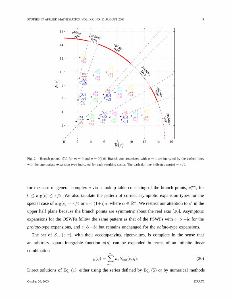
Fig. 2. Branch points, cmn◦;r for m = 0 and n = 0(1)6. Branch cuts associated with n = 4 are indicated by the dashed lines

with the appropriate expansion type indicated for each resulting sector. The dash-dot line indicates arg(c) = π/4.

for the case of general complex c via a lookup table consisting of the branch points, cmn◦;r , for

0 ≤ arg(c) ≤ π/2. We also tabulate the pattern of correct asymptotic expansion types for the

special case of arg(c) = π/4 or c = (1+i)α, where α ∈ <+. We restrict our attention to c2 in the

upper half plane because the branch points are symmetric about the real axis [36]. Asymptotic

expansions for the OSWFs follow the same pattern as that of the PSWFs with c⇒ −ic for the

prolate-type expansions, and c 6⇒ −ic but remains unchanged for the oblate-type expansions.

The set of Smn(c, η), with their accompanying eigenvalues, is complete in the sense that

an arbitrary square-integrable function y(η) can be expanded in terms of an infinite linear

combination

y(η) =∞

∑

n=m

anSmn(c, η). (20)

Direct solutions of Eq. (1), either using the series defined by Eq. (5) or by numerical methods



such as a Runge-Kutta method, are unambiguous and theoretically valid for any m, n, and c.

However, the spheroidal eigenvalues develop square root branch cuts where the solution to the

infinite continued fraction equation, or equivalently the characteristic eigenvalue equation (e.g

from Hodge’s method), becomes degenerate and possesses double roots [52].

At these branch points, cmn◦;r , two spheroidal eigenvalues merge and become analytic contin-

uations of each other [36], [37]. One consequence of this is that, as the eigenvalues exchange

identities by level crossing onto each other’s Riemann sheet, their respective asymptotic expan-

sions are also interchanged. Thus λmn and Smn(c, η) are described alternately by a prolate-type

asymptotic expansion then an oblate-type asymptotic expansion, as arg(c) (starting at arg(c) = 0)

crosses the branch cuts (emanating radially outward from cmn◦;r ) associated with a particular m

and n. Given c, m, n, and cmn◦;r therefore, a simple lookup table determines which asymptotic

expansion is appropriate by comparing arg(c) to arg(cmn◦;r ). These transitions are depicted in

Fig. 2, which shows the branch cuts and their appropriate asymptotic expansion regions for

m = 0 and n = 4. As arg(c) progresses from 0 to π/2, each corresponding λmn crosses branch

cuts (roughly proportional in number to n+1) and alternates expansion type with each crossing.

At arg(c) = 0, all λmn are prolate-type, at arg(c) = π/2, all λmn are oblate-type, while at

arg(c) = π/4, the λmn are divided evenly between prolate and oblate types (see Fig. 4).

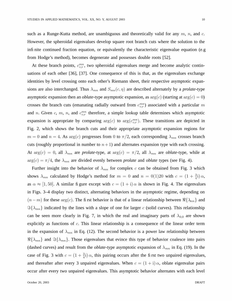
Further insight into the behavior of λmn for complex c can be obtained from Fig. 3 which

shows λmn calculated by Hodge’s method for m = 0 and n = 0(1)20 with c = (1 + 34i)α,

as α ≈ [1, 50]. A similar figure except with c = (1 + i)α is shown in Fig. 4. The eigenvalues

in Figs. 3–4 display two distinct, alternating behaviors in the asymptotic regime, depending on

(n−m) for these arg(c). The first behavior is that of a linear relationship between <{λmn} and

={λmn} indicated by the lines with a slope of one for larger c (solid curves). This relationship

can be seen more clearly in Fig. 7, in which the real and imaginary parts of λ0,0 are shown

explicitly as functions of c. This linear relationship is a consequence of the linear order term

in the expansion of λmn in Eq. (12). The second behavior is a power law relationship between

<{λmn} and ={λmn}. Those eigenvalues that evince this type of behavior coalesce into pairs

(dashed curves) and result from the oblate-type asymptotic expansion of λmn in Eq. (19). In the

case of Fig. 3 with c = (1 + 34i)α, this pairing occurs after the first two unpaired eigenvalues,

and thereafter after every 3 unpaired eigenvalues. When c = (1 + i)α, oblate eigenvalue pairs

occur after every two unpaired eigenvalues. This asymptotic behavior alternates with each level



100

101

102

103

101

102

103

PSfrag replacements

λ0,0 λ0,1

8

λ0,1

4

λ0,1

1

λ0,9

λ0,3

λ0,2

λ0,1

<{λ0,0(1)18((1 + i)[1.6, 50])}

={λ

0,0

(1)1

8((

1+

i)[1.6,5

0])}

c = (1 + 34i)1.6

c = (1 + 34i)50

log10(={λmn})log10(<{λmn})

' 1.2

log

10(=

{λm

n})

log

10(<

{λm

n})

'1

2

Fig. 3. λmn: Eigenvalues of the spheroidal wave equation. m = 0 and n = 0(1)18. Each curve tracks an eigenvalue as c

ranges from c = (1 + 34i)1.6 (lower end of each curve) to c = (1 + 3

4i)50 (upper end of each curve). Dashed curves indicate

coalescing oblate eigenvalue pairs. The “2” indicates λ0,2((1 + 34i)50).

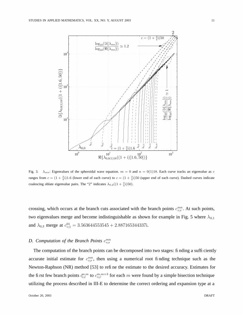
crossing, which occurs at the branch cuts associated with the branch points cmn◦;r . At such points,

two eigenvalues merge and become indistinguishable as shown for example in Fig. 5 where λ0,1

and λ0,3 merge at c01◦;1 = 3.563644553545 + 2.887165344337i.

D. Computation of the Branch Points cmn◦;r

The computation of the branch points can be decomposed into two stages: finding a sufficiently

accurate initial estimate for cmn◦;r , then using a numerical root finding technique such as the

Newton-Raphson (NR) method [53] to refine the estimate to the desired accuracy. Estimates for

the first few branch points cm,m◦;r to cm,m+3

◦;r for each m were found by a simple bisection technique

utilizing the process described in III-E to determine the correct ordering and expansion type at a



100

101

102

101

102

103

101

101

PSfrag replacements

λ0,0 λ0,1

8

λ0,1

4

λ0,1

1

λ0,8λ0,2λ0,1

<{λ0,0(1)18((1 + i)[1.7, 50])}

={λ

0,0

(1)1

8((

1+

i)[1.7,5

0])}

c = (1 + i)1.7

c = (1 + i)50

log

10(=

{λm

n})

log

10(<

{λm

n})

'2

log

10(=

{λm

n})

log

10(<

{λm

n})

'1

Fig. 4. λmn: Eigenvalues of the spheroidal wave equation. m = 0 and n = 0(1)18. Each curve tracks an eigenvalue as c

ranges from c = (1 + i)1.7 (lower end of each curve) to c = (1 + i)50 (upper end of each curve). Dashed curves indicate

coalescing oblate eigenvalue pairs.

given c. The bisection technique tested successively narrower sectors of arg(c) in order to specify

the approximate angle at which the asymptotic expansions for λm,n and λm,n+2 interchanged.

Once the initial guess for arg(cmn◦;r ) was found to the desired accuracy, |cmn

◦;r | was searched for

between 0 and n + 15 (as an approximate upper bound) using a simplex search method [54]

based on finding the minimum |λm,n − λm,n+2| for the merging pair. After accurate cm,m..m+1◦;r

were found in this manner, initial guesses for arg(cm,m+2..m+3◦;r ) were obtained also via bisection

by noting that arg(cm,n+2◦;r,odd ) are interspersed with arg(cm,n

◦;r,even), thus providing upper and lower

bounds in arg(c) for the bisection method. An estimate for |cm,m+2..m+3◦;r | was obtained by noting



101

101

102

PSfrag replacements

λ0,0

λ0,18

λ0,14

λ0,11

λ0,8

λ0,7

λ0,6

λ0,5

λ0,4

λ0,3λ

0,2

λ0,1

<{λ0,0(1)8((c01◦;1/|c01◦;1|)[3, 12])}

={λ

0,0

(1)8

((c0

1 ◦;1/|c0

1 ◦;1|)[

3,12

])}

c = (c01◦;1/|c01◦;1|)3

c = (c01◦;1/|c01◦;1|)12


' 2


' 1

Fig. 5. Branch point c0,1◦;1 = c0,3

◦;2 = 3.563644553545 + 2.887165344337i where λ0,1 and λ0,3 merge at λ0,1◦;1 = λ0,3

◦;2 =

10.1408387872326 + 11.1215866842249i. Dashed curves indicate coalescing oblate eigenvalue pairs.

that

min(∣

∣cm,n+2◦;r,odd

∣

∣

)

> max(∣

∣cm,n+2◦;r,even

∣

∣ =∣

∣cm,n◦;r,odd

∣

∣

)

(21)

and by observing the pattern which soon becomes apparent (see Fig. 2). Initial estimates for the

remaining cm,m+4...◦;r were based on simple polynomial estimation techniques.

These initial guesses for cmn◦;r were then used as a starting point for a quadruple precision

multivariate (in λ and c2) NR root finding technique [36]. In most cases, these initial guesses

were sufficiently accurate for the convergence of the NR method. Those that were not of

sufficient accuracy were first refined using a simplex search method, which has a larger radius of

convergence, prior to invoking the NR method. In all cases, this combined numerical procedure



correctly and exhaustively identified the branch points for m ≤ n ≤ 59 as well as m = 0(1)10,

n ≤ 100. The accuracy as defined by the smallest correction of the NR method was less than

1×10−15 in the vast majority of cases. However, as n increased, the accuracy of the NR method

decreased until, for example, of c0,100◦;r ≈ 1 × 10−8. This numerical procedure for finding initial

guesses is an alternative to the WKBJ, or phase-integral, method outlined in [36]. A brief table

of these results is given as Table II while a more complete listing is provided in [55]. The

programs used in this calculation may be obtained by contacting the author.

E. Eigenvalue Ordering for Complex c

For purely real, purely imaginary, or sufficiently small complex c, the ordering (indexed by

n) is determined by the absolute magnitude of λmn [46]. However, for larger complex c, the

eigenvalues may no longer be sorted merely by |λmn|. The power law nature of the imaginary

part of those coalescing eigenvalues, when compared to the real part, especially in the asymptotic

regime (large c), soon dominates and disrupts ordering by |λmn| (see Fig. 6). A better choice for

deciding the ordering of λmn seems to be <{λmn} due to its linear increase in the asymptotic

regime, for both types of behaviors noted above. Yet this choice of ordering is also not correct

as coalescing oblate pairs of eigenvalues often reverse order, according to this measure, before

becoming indistinguishable (see Fig 4 and inset therein). Additionally, ordering by <{λmn} fails

for cases of general c such as c = (1+ 34i)α, as can be seen by comparing Fig. 3 with Fig. 6. To

illustrate the difficulty associated with eigenvalue ordering, note the eigenvalue corresponding

to the asterisk labeled “λ0,2” in Figs. 3 and 6. This eigenvalue is assigned order n = 7 by an

eigenvalue solver in Hodge’s method, n = 12 when arranged according to increasing |<{λmn}|,n = 52 when arranged according to |λmn|, while inspection of Fig. 3 reveals that this eigenvalue

should in fact correspond to order n = 2.

At least it can be said that the eigenvalue ordering and expansion patterns for general, complex

c should follow the ordering for λmn when c = 0. At that point, the eigenvalues reduce to

λmn(c = 0) = n(n+ 1), n ≥ m, (22)

and the spheroidal wave equation (1) reduces to the equation satisfied by the associated Legendre

functions of the first kind of integral order and degree, Pmn (η). This fact is sufficient to suggest

a brute force method for finding λmn ordering and expansion type for large, complex values of



m n r cm,n◦;r = cm,n+2

◦;r+1 λm,n◦;r = λm,n+2

◦;r+1

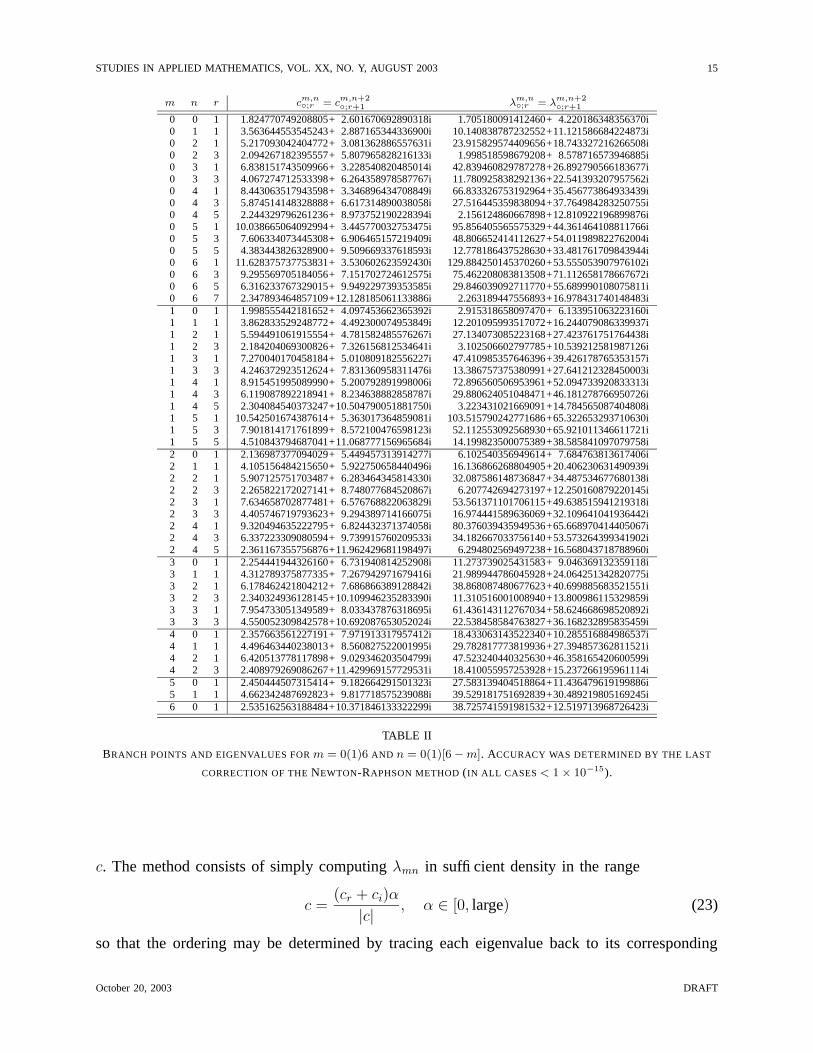
0 0 1 1.824770749208805+ 2.601670692890318i 1.705180091412460+ 4.220186348356370i0 1 1 3.563644553545243+ 2.887165344336900i 10.140838787232552+11.121586684224873i0 2 1 5.217093042404772+ 3.081362886557631i 23.915829574409656+18.743327216266508i0 2 3 2.094267182395557+ 5.807965828216133i 1.998518598679208+ 8.578716573946885i0 3 1 6.838151743509966+ 3.228540820485014i 42.839460829787278+26.892790566183677i0 3 3 4.067274712533398+ 6.264358978587767i 11.780925838292136+22.541393207957562i0 4 1 8.443063517943598+ 3.346896434708849i 66.833326753192964+35.456773864933439i0 4 3 5.874514148328888+ 6.617314890038058i 27.516445359838094+37.764984283250755i0 4 5 2.244329796261236+ 8.973752190228394i 2.156124860667898+12.810922196899876i0 5 1 10.038665064092994+ 3.445770032753475i 95.856405565575329+44.361464108811766i0 5 3 7.606334073445308+ 6.906465157219409i 48.806652414112627+54.011989822762004i0 5 5 4.383443826328900+ 9.509669337618593i 12.778186437528630+33.481761709843944i0 6 1 11.628375737753831+ 3.530602623592430i 129.884250145370260+53.555053907976102i0 6 3 9.295569705184056+ 7.151702724612575i 75.462208083813508+71.112658178667672i0 6 5 6.316233767329015+ 9.949229739353585i 29.846039092711770+55.689990108075811i0 6 7 2.347893464857109+12.128185061133886i 2.263189447556893+16.978431740148483i1 0 1 1.998555442181652+ 4.097453662365392i 2.915318658097470+ 6.133951063223160i1 1 1 3.862833529248772+ 4.492300074953849i 12.201095993517072+16.244079086339937i1 2 1 5.594491061915554+ 4.781582485576267i 27.134073085223168+27.423761751764438i1 2 3 2.184204069300826+ 7.326156812534641i 3.102506602797785+10.539212581987126i1 3 1 7.270040170458184+ 5.010809182556227i 47.410985357646396+39.426178765353157i1 3 3 4.246372923512624+ 7.831360958311476i 13.386757375380991+27.641212328450003i1 4 1 8.915451995089990+ 5.200792891998006i 72.896560506953961+52.094733920833313i1 4 3 6.119087892218941+ 8.234638882858787i 29.880624051048471+46.181278766950726i1 4 5 2.304084540373247+10.504790051881750i 3.223431021669091+14.784565087404808i1 5 1 10.542501674387614+ 5.363017364859081i 103.515790242771686+65.322653293710630i1 5 3 7.901814171761899+ 8.572100476598123i 52.112553092568930+65.921011346611721i1 5 5 4.510843794687041+11.068777156965684i 14.199823500075389+38.585841097079758i2 0 1 2.136987377094029+ 5.449457313914277i 6.102540356949614+ 7.684763813617406i2 1 1 4.105156484215650+ 5.922750658440496i 16.136866268804905+20.406230631490939i2 2 1 5.907125751703487+ 6.283464345814330i 32.087586148736847+34.487534677680138i2 2 3 2.265822172027141+ 8.748077684520867i 6.207742694273197+12.250160879220145i2 3 1 7.634658702877481+ 6.576768822063829i 53.561371101706115+49.638515941219318i2 3 3 4.405746719793623+ 9.294389714166075i 16.974441589636069+32.109641041936442i2 4 1 9.320494635222795+ 6.824432371374058i 80.376039435949536+65.668970414405067i2 4 3 6.337223309080594+ 9.739915760209533i 34.182667033756140+53.573264399341902i2 4 5 2.361167355756876+11.962429681198497i 6.294802569497238+16.568043718788960i3 0 1 2.254441944326160+ 6.731940814252908i 11.273739025431583+ 9.046369132359118i3 1 1 4.312789375877335+ 7.267942971679416i 21.989944786045928+24.064251342820775i3 2 1 6.178462421804212+ 7.686866389128842i 38.868087480677623+40.699885683521551i3 2 3 2.340324936128145+10.109946235283390i 11.310516001008940+13.800986115329859i3 3 1 7.954733051349589+ 8.033437876318695i 61.436143112767034+58.624668698520892i3 3 3 4.550052309842578+10.692087653052024i 22.538458584763827+36.168232895835459i4 0 1 2.357663561227191+ 7.971913317957412i 18.433063143522340+10.285516884986537i4 1 1 4.496463440238013+ 8.560827522001995i 29.782817773819936+27.394857362811521i4 2 1 6.420513778117898+ 9.029346203504799i 47.523240440325630+46.358165420600599i4 2 3 2.408979269086267+11.429969157729531i 18.410055957253928+15.237266195961114i5 0 1 2.450444507315414+ 9.182664291501323i 27.583139404518864+11.436479619199886i5 1 1 4.662342487692823+ 9.817718575239088i 39.529181751692839+30.489219805169245i6 0 1 2.535162563188484+10.371846133322299i 38.725741591981532+12.519713968726423i

TABLE II

BRANCH POINTS AND EIGENVALUES FOR m = 0(1)6 AND n = 0(1)[6 − m]. ACCURACY WAS DETERMINED BY THE LAST

CORRECTION OF THE NEWTON-RAPHSON METHOD (IN ALL CASES < 1 × 10−15).

c. The method consists of simply computing λmn in sufficient density in the range

c =(cr + ci)α

|c| , α ∈ [0, large) (23)

so that the ordering may be determined by tracing each eigenvalue back to its corresponding



0 500 1000 1500 2000 2500 3000 3500 40000

500

1000

1500

2000

2500

3000

3500

4000

PSfrag replacements

<{λ0,0(1)58((1 + 34i)50)}

={λ

0,0

(1)5

8((

1+

3 4i)50

)}

λ0,0λ0,1

λ0,2, λ0,3

λ0,4λ0,5λ0,6

λ0,7, λ0,8

λ0,9λ0,10λ0,11

λ0,12, λ0,13

λ0,14λ0,15λ0,16

λ0,17, λ0,18

λ0,19λ0,20λ0,21

λ0,22, λ0,23

λ0,24λ0,25λ0,26

λ0,27, λ0,28

λ0,29λ0,30λ0,31

λ0,32, λ0,33

λ0,34λ0,35λ0,36

λ0,37, λ0,38

λ0,39λ0,40λ0,41

λ0,42, λ0,43

λ0,4

6

λ0,4

9

λ0,5

2

λ0,5

5

λ0,5

8

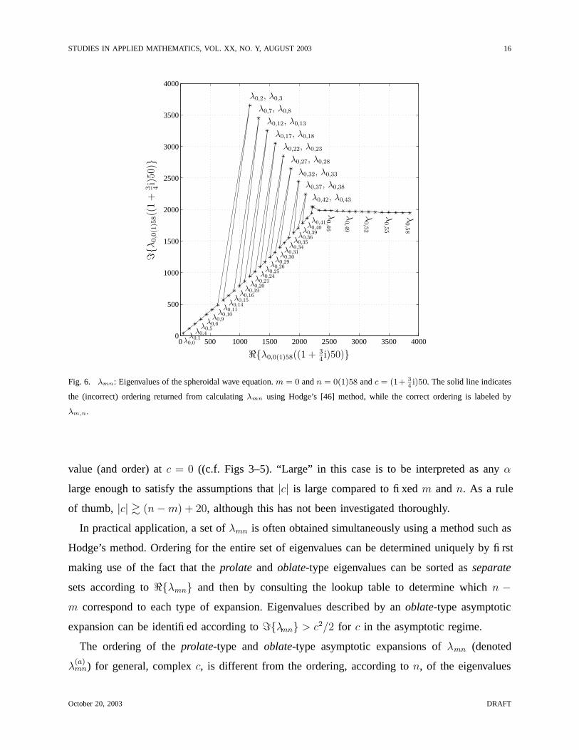
Fig. 6. λmn: Eigenvalues of the spheroidal wave equation. m = 0 and n = 0(1)58 and c = (1+ 34i)50. The solid line indicates

the (incorrect) ordering returned from calculating λmn using Hodge’s [46] method, while the correct ordering is labeled by

λm,n.

value (and order) at c = 0 ((c.f. Figs 3–5). “Large” in this case is to be interpreted as any α

large enough to satisfy the assumptions that |c| is large compared to fixed m and n. As a rule

of thumb, |c| & (n−m) + 20, although this has not been investigated thoroughly.

In practical application, a set of λmn is often obtained simultaneously using a method such as

Hodge’s method. Ordering for the entire set of eigenvalues can be determined uniquely by first

making use of the fact that the prolate and oblate-type eigenvalues can be sorted as separate

sets according to <{λmn} and then by consulting the lookup table to determine which n −m correspond to each type of expansion. Eigenvalues described by an oblate-type asymptotic

expansion can be identified according to ={λmn} > c2/2 for c in the asymptotic regime.

The ordering of the prolate-type and oblate-type asymptotic expansions of λmn (denoted

λ(a)mn) for general, complex c, is different from the ordering, according to n, of the eigenvalues



themselves. While the n indicates λmn ordering for each m, the λ(a)mn are ordered according

to m, but independently, corresponding to the sequential ordering for each type of expansion

separately. Let np be the number of prolate-type expansions of λmn necessary up to but excluding

n, and no be the number of oblate-type expansions of λmn necessary up to but excluding n. λmn

can then be approximated by prolate-type λ(a)mn ordered according to np beginning at np = m,

and oblate-type λ(a)mn ordered according to no beginning at no = m, interspersed in a pattern

determined by arg(c) via the lookup table described in Section III-C.

As an illustration, for the case of c of the form c = (1 + i)α, λ0,0 would correspond to the

zeroth (np = 0) prolate-type asymptotic expansion. On the other hand, the second eigenvalue

for m = 0, λ0,1, coalesces with the third eigenvalue, λ0,2 (see Fig. 4), and these correspond to

the zeroth (no = 0) and first (no = 1) oblate-type asymptotic expansions respectively. To be

specific, we explicitly show the dependence of Γk on m and n, and express the prolate-type

expansion of λ(a)0,0 from Eq. (12) as

λ0,0 ≈ λ(a)0,0 =

∞∑

k=0

Γk(m = 0, n⇒ np = 0)c−k+1. (24)

For completeness, we also show the oblate-type expansion of λ(a)0,1 and λ(a)

0,2 from Eq. (19) as

λ0,1 ≈ λ(a)0,1 =

∞∑

k=0

Γk(m = 0, n⇒ no = 0)(−ic)−k+2. (25a)

λ0,2 ≈ λ(a)0,2 =

∞∑

k=0

Γk(m = 0, n⇒ no = 1)(−ic)−k+2. (25b)

In turn the fourth eigenvalue, λ0,3, corresponds to the first (np = 1) prolate-type asymptotic

expansion, and so on (c.f. Fig. 4). The oblate spheroidal eigenvalues are also expressed in

terms of either the prolate-type and oblate-type asymptotic expansions, however, c ⇒ (−ic)

in Eq. (24) while (−ic) ⇒ c in Eq. (25a). The ordering of the prolate-type and oblate-type

asymptotic expansions in Section III as applied to the OSWFs also adhere to this alternating

pattern according to np and no.

Table III details which type of asymptotic expansion of the prolate spheroidal eigenvalue λmn

is appropriate for a given m and n and indicates the ordering aspects of these expansions for

the specific cases of m = 0(1)2, (n − m) = 0(1)8, and c of the form c = (1 + i)α. For this

case, the first m+1 expansions of λmn are prolate-type expansions after which alternating pairs



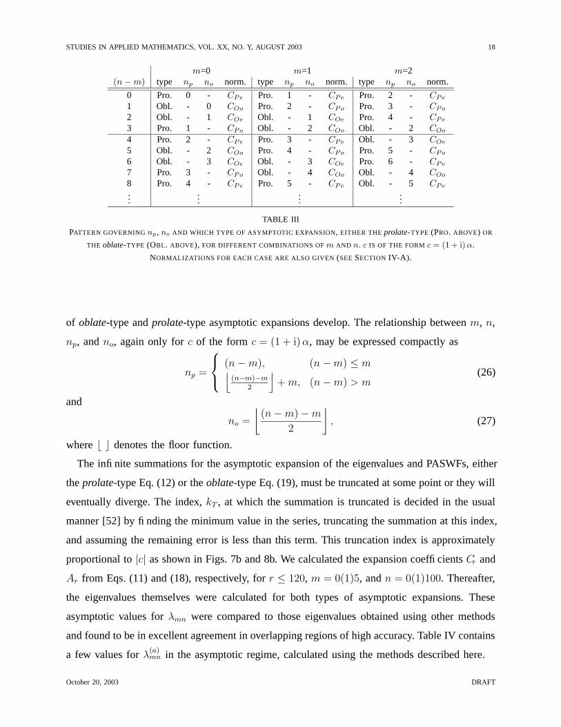
m=0 m=1 m=2(n − m) type np no norm. type np no norm. type np no norm.

0 Pro. 0 - CPe Pro. 1 - CPe Pro. 2 - CPe

1 Obl. - 0 COo Pro. 2 - CPo Pro. 3 - CPo

2 Obl. - 1 COe Obl. - 1 COe Pro. 4 - CPe

3 Pro. 1 - CPo Obl. - 2 COo Obl. - 2 COo

4 Pro. 2 - CPe Pro. 3 - CPe Obl. - 3 COe

5 Obl. - 2 COo Pro. 4 - CPo Pro. 5 - CPo

6 Obl. - 3 COe Obl. - 3 COe Pro. 6 - CPe

7 Pro. 3 - CPo Obl. - 4 COo Obl. - 4 COo

8 Pro. 4 - CPe Pro. 5 - CPe Obl. - 5 CPe

......

......

TABLE III

PATTERN GOVERNING np , no AND WHICH TYPE OF ASYMPTOTIC EXPANSION, EITHER THE prolate-TYPE (PRO. ABOVE) OR

THE oblate-TYPE (OBL. ABOVE), FOR DIFFERENT COMBINATIONS OF m AND n. c IS OF THE FORM c = (1 + i) α.

NORMALIZATIONS FOR EACH CASE ARE ALSO GIVEN (SEE SECTION IV-A).

of oblate-type and prolate-type asymptotic expansions develop. The relationship between m, n,

np, and no, again only for c of the form c = (1 + i)α, may be expressed compactly as

np =

(n−m), (n−m) ≤ m⌊

(n−m)−m2

⌋

+m, (n−m) > m(26)

and

no =

⌊

(n−m) −m

2

⌋

, (27)

where b c denotes the floor function.

The infinite summations for the asymptotic expansion of the eigenvalues and PASWFs, either

the prolate-type Eq. (12) or the oblate-type Eq. (19), must be truncated at some point or they will

eventually diverge. The index, kT , at which the summation is truncated is decided in the usual

manner [52] by finding the minimum value in the series, truncating the summation at this index,

and assuming the remaining error is less than this term. This truncation index is approximately

proportional to |c| as shown in Figs. 7b and 8b. We calculated the expansion coefficients Cr and

Ar from Eqs. (11) and (18), respectively, for r ≤ 120, m = 0(1)5, and n = 0(1)100. Thereafter,

the eigenvalues themselves were calculated for both types of asymptotic expansions. These

asymptotic values for λmn were compared to those eigenvalues obtained using other methods

and found to be in excellent agreement in overlapping regions of high accuracy. Table IV contains

a few values for λ(a)mn in the asymptotic regime, calculated using the methods described here.



1 2 3 4 5 6 7

0

1

2

3

4

5

6

7

1 2 3 4 5 6 7

10−5

100

5

10

15

20

PSfrag replacements

<{c}

a)Pr

olat

eei

genv

alue

,λ

0,0

b)

∣ ∣ ∣ ∣

λ0,0−

λ(a

)0,0

λ0,0

∣ ∣ ∣ ∣

kT

inE

q.(12)

<{λ0,0}={λ0,0}<{λ(a)

0,0}={λ(a)

0,0}

|<{(λ0,0 − λ(a)0,0)/λ0,0}|

|={(λ0,0 − λ(a)0,0)/λ0,0}|

kT

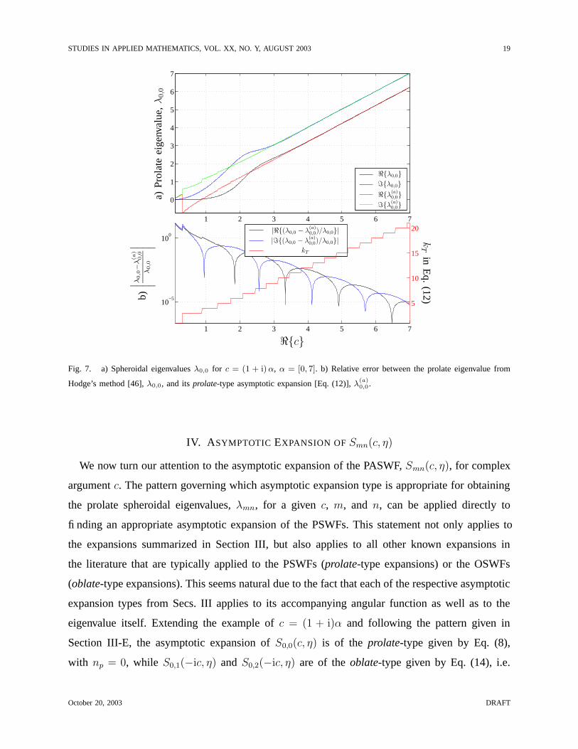
Fig. 7. a) Spheroidal eigenvalues λ0,0 for c = (1 + i) α, α = [0, 7]. b) Relative error between the prolate eigenvalue from

Hodge’s method [46], λ0,0, and its prolate-type asymptotic expansion [Eq. (12)], λ(a)0,0 .

IV. ASYMPTOTIC EXPANSION OF Smn(c, η)

We now turn our attention to the asymptotic expansion of the PASWF, Smn(c, η), for complex

argument c. The pattern governing which asymptotic expansion type is appropriate for obtaining

the prolate spheroidal eigenvalues, λmn, for a given c, m, and n, can be applied directly to

finding an appropriate asymptotic expansion of the PSWFs. This statement not only applies to

the expansions summarized in Section III, but also applies to all other known expansions in

the literature that are typically applied to the PSWFs (prolate-type expansions) or the OSWFs

(oblate-type expansions). This seems natural due to the fact that each of the respective asymptotic

expansion types from Secs. III applies to its accompanying angular function as well as to the

eigenvalue itself. Extending the example of c = (1 + i)α and following the pattern given in

Section III-E, the asymptotic expansion of S0,0(c, η) is of the prolate-type given by Eq. (8),

with np = 0, while S0,1(−ic, η) and S0,2(−ic, η) are of the oblate-type given by Eq. (14), i.e.



1 2 3 4 5 6 7

10−5

100

0

10

20

30

401 2 3 4 5 6 7

0

10

20

30

40

50

60

70

80

0.5 1 1.5 2 2.5

0

2

4

6

8

PSfrag replacements

<{c}

a)Pr

olat

eei

genv

alue

,λ

0,1

b)

∣ ∣ ∣ ∣

λ0,1−

λ(a

)0,1

λ0,1

∣ ∣ ∣ ∣

kT

inE

q.(19)

<{λ0,1}={λ0,1}<{λ(a)

0,1}={λ(a)

0,1}

|<{(λ0,1 − λ(a)0,1)/λ0,1}|

|={(λ0,1 − λ(a)0,1)/λ0,1}|

kT

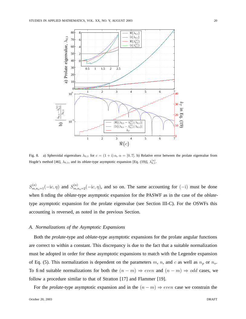
Fig. 8. a) Spheroidal eigenvalues λ0,1 for c = (1 + i) α, α = [0, 7]. b) Relative error between the prolate eigenvalue from

Hogde’s method [46], λ0,1, and its oblate-type asymptotic expansion [Eq. (19)], λ(a)0,1 .

S(a)m,no=1(−ic, η) and S

(a)m,no=2(−ic, η), and so on. The same accounting for (−i) must be done

when finding the oblate-type asymptotic expansion for the PASWF as in the case of the oblate-

type asymptotic expansion for the prolate eigenvalue (see Section III-C). For the OSWFs this

accounting is reversed, as noted in the previous Section.

A. Normalizations of the Asymptotic Expansions

Both the prolate-type and oblate-type asymptotic expansions for the prolate angular functions

are correct to within a constant. This discrepancy is due to the fact that a suitable normalization

must be adopted in order for these asymptotic expansions to match with the Legendre expansion

of Eq. (5). This normalization is dependent on the parameters m, n, and c as well as np or no.

To find suitable normalizations for both the (n − m) ⇒ even and (n − m) ⇒ odd cases, we

follow a procedure similar to that of Stratton [17] and Flammer [19].

For the prolate-type asymptotic expansion and in the (n−m) ⇒ even case we constrain the



value of the asymptotic expansion at η = 0 to be equal to the associated Legendre function of

degree n and order m,

Smn(c, 0) ≈ CPe

[ ∞∑′

r=−∞CrDnp−m+r(0)

]

= Pmn (0) (28)

where we have extracted the normalizing constant CPe. Note that np has been inserted into

the parabolic cylinder expansion reflecting the fact that this is only for prolate-type asymptotic

expansions and therefore ordering must be according to np instead of n. The associated Legendre

function Pmn (η) retains n as the order because this index is specified by the n of Smn(c, η). Based

on the expressions for the Legendre and parabolic cylinder functions of zero argument [42], CPe

becomes

CPe =

[

(−1)n−m

2 (n+m)!]

/[

2n(

n−m2

)

!(

n+m2

)

!]

∞∑′

r=−∞Cr

√π

2−(np−m+r)

2 Γ(

1−(np−m+r)

2

)

(29)

where Γ refers to the Gamma function [42].

When (n−m) ⇒ odd, we constrain the value of the first derivative of the asymptotic expansion

at η = 0 to be equal to the derivative of the associated Legendre function of degree n and order

m,

S ′mn(c, 0) ≈ CPo

∂

∂η

[

(1 − η2)m2

∞∑′

r=−∞CrDnp−m+r

(

η√

2c)

]∣

∣

∣

∣

∣

η=0

= Pm′n (0) (30)

having extracted the normalizing constant CPo. The derivative of the left side of Eq. (30) can

be expressed as

(1−η2)m2

[ ∞∑′

r=−∞Cr

[

D′np−m+r

(

η√

2c)]√

2c

]

+

[ ∞∑′

r=−∞CrDnp−m+r

(

η√

2c)

]

m

2(1−η2)

m2−1(−2η).

(31)

When η = 0 in Eq. (31), the normalization constant for the prolate-type asymptotic expansion

for (n−m) ⇒ odd becomes

CPo =

[

(−1)n−m−1

2 (n+m+ 1)!]

/[

2n(

n−m−12

)

!(

n+m+12

)

!]

−∞

∑′

r=−∞Cr

√2cπ

2−(np−m+r+1)

2 Γ(

−(np−m+r)

2

)

. (32)

The oblate-type asymptotic expansions of the PASWF require similar normalizations. When

(n −m) ⇒ even, we constrain the value of the oblate-type asymptotic expansion at η = 0 to



be equal to the associated Legendre function of degree n and order m,

Smn(−ic, 0) ≈ COe

[ ∞∑

r=−ν

Ar

{

eicL(m)ν+r (−i2c) + (−1)n−meicL

(m)ν+r (−i2c)

}

]

= Pmn (0). (33)

where ν is now defined as

ν =

no−m2, (n−m) even

no−m−12

, (n−m) odd.(34)

It is important to note that the n in the factor (−1)n−m in Eqs. (33) and (37) remains the n of

the prolate angular function, Smn(−ic, η) (as opposed to being replaced by no), because it is

introduced to assure the symmetry or antisymmetry of the prolate angular functions. Therefore

it remains associated with them rather than with the oblate-type asymptotic expansion. In this

case, since (n−m) ⇒ even, Eq. (33) reduces to

Smn(−ic, η) ≈ COe

[ ∞∑

r=−ν

Ar2 eicL

(m)ν+r(−i2c)

]

= Pmn (0). (35)

Thus, the normalization constant, COe, for the oblate-type asymptotic expansion, (n − m) ⇒even, is

COe =

[

(−1)n−m

2 (n+m)!]

/[

2n(

n−m2

)

!(

n+m2

)

!]

2eic

∞∑

r=−ν

ArL(m)ν+r(−i2c)

(36)

Finally, the normalization constant for the oblate-type asymptotic expansion when (n−m) ⇒odd can be found by constraining the value of the first derivative of the asymptotic expansion

at η = 0 to be equal to the derivative of the associated Legendre function of degree n and order

m,

S ′mn(−ic, 0) ≈

COo∂

∂η

[

(1 − η2)m2

∞∑

r=−ν

Ar

{

L(m)ν+r [−i2c(1 − η)]

e−ic(1−η)+ (−1)n−mL

(m)ν+r [−i2c(1 + η)]

e−ic(1+η)

}]∣

∣

∣

∣

∣

η=0

= Pm′n (0).(37)

After taking the derivative of the left side of Eq. (37) and letting η = 0, one obtains the

normalization constant for the oblate-type asymptotic expansion for (n−m) ⇒ odd as

COo =

[

(−1)n−m−1

2 (n+m+ 1)!]

/[

2n(

n−m−12

)

!(

n+m+12

)

!]

−i2c eic

∞∑

r=−ν

Ar

{

L(m)ν+r(−i2c) − 2L

(m)′ν+r (−i2c)

}

. (38)



0 0.1 0.2 0.3 0.4 0.5 0.6 0.7 0.8 0.9 1−1

−0.5

0

0.5

1

0 0.1 0.2 0.3 0.4 0.5 0.6 0.7 0.8 0.9 1

10−15

10−10

PSfrag replacements

Angular coordinate (η)

a)S

0,(0,3

,4)(

(1+

i)20,η

)b)

∣ ∣ ∣S

0,(0,3

,4)−S

(a)

0,(0,3

,4)∣ ∣ ∣

<{S0,0((1+i)20, η)}={S0,0((1+i)20, η)}<{S0,3((1+i)20, η)}={S0,3((1+i)20, η)}<{S0,4((1+i)20, η)}={S0,4((1+i)20, η)}

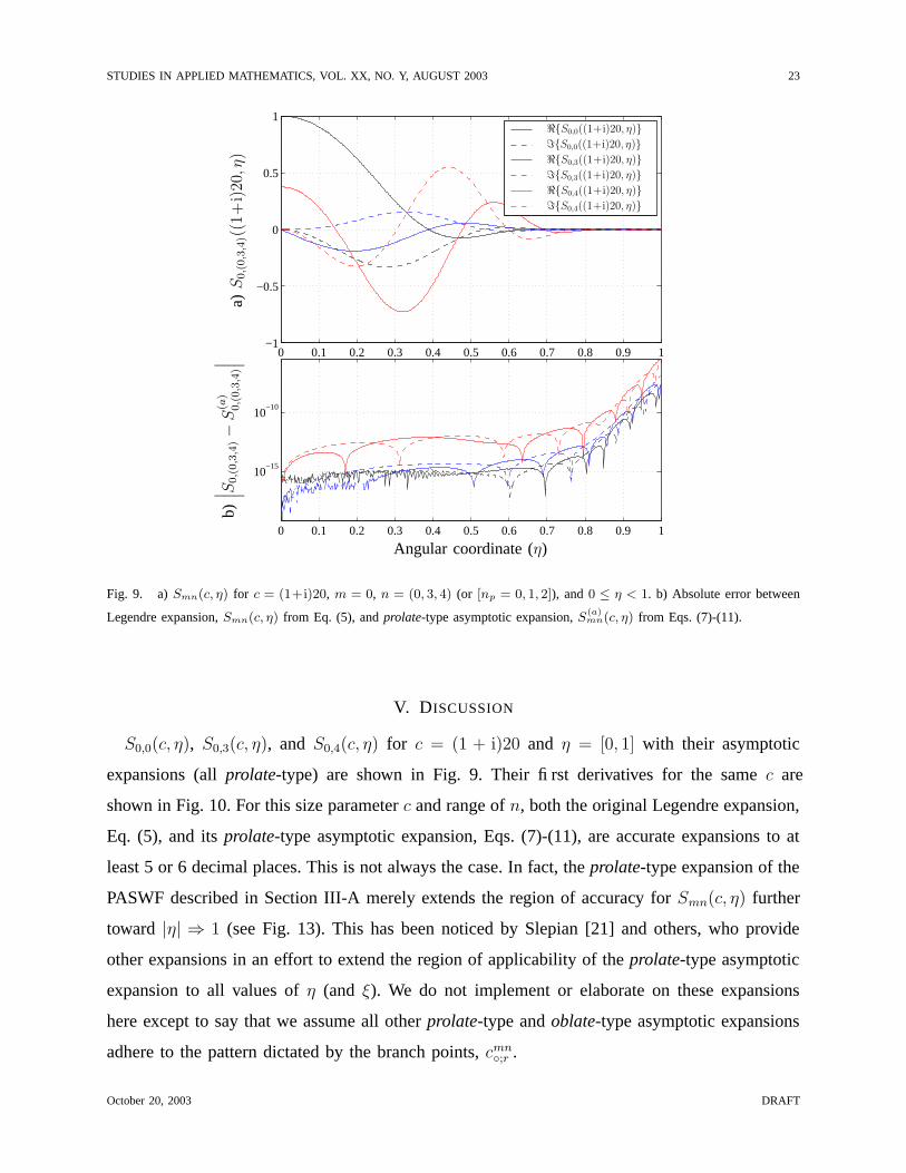
Fig. 9. a) Smn(c, η) for c = (1+i)20, m = 0, n = (0, 3, 4) (or [np = 0, 1, 2]), and 0 ≤ η < 1. b) Absolute error between

Legendre expansion, Smn(c, η) from Eq. (5), and prolate-type asymptotic expansion, S(a)mn(c, η) from Eqs. (7)-(11).

V. DISCUSSION

S0,0(c, η), S0,3(c, η), and S0,4(c, η) for c = (1 + i)20 and η = [0, 1] with their asymptotic

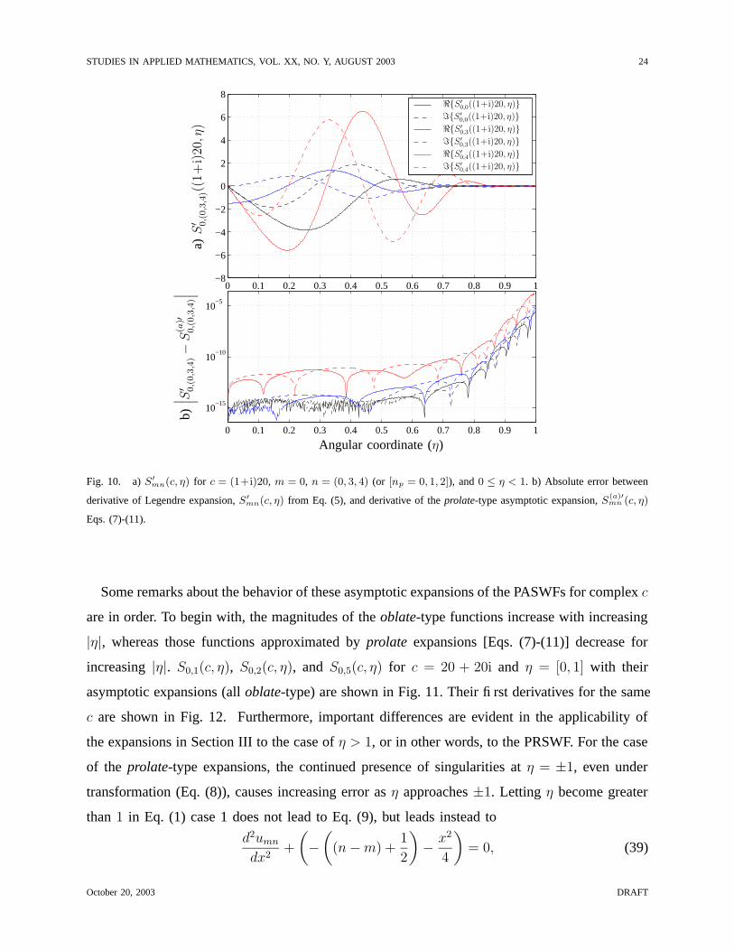
expansions (all prolate-type) are shown in Fig. 9. Their first derivatives for the same c are

shown in Fig. 10. For this size parameter c and range of n, both the original Legendre expansion,

Eq. (5), and its prolate-type asymptotic expansion, Eqs. (7)-(11), are accurate expansions to at

least 5 or 6 decimal places. This is not always the case. In fact, the prolate-type expansion of the

PASWF described in Section III-A merely extends the region of accuracy for Smn(c, η) further

toward |η| ⇒ 1 (see Fig. 13). This has been noticed by Slepian [21] and others, who provide

other expansions in an effort to extend the region of applicability of the prolate-type asymptotic

expansion to all values of η (and ξ). We do not implement or elaborate on these expansions

here except to say that we assume all other prolate-type and oblate-type asymptotic expansions

adhere to the pattern dictated by the branch points, cmn◦;r .



0 0.1 0.2 0.3 0.4 0.5 0.6 0.7 0.8 0.9 1−8

−6

−4

−2

0

2

4

6

8

0 0.1 0.2 0.3 0.4 0.5 0.6 0.7 0.8 0.9 1

10−15

10−10

10−5

PSfrag replacements


a)S′ 0,(0,3

,4)(

(1+

i)20,η

)b)

∣ ∣ ∣S′ 0,(0,3

,4)−S

(a)′

0,(0,3

,4)∣ ∣ ∣

<{S ′0,0((1+i)20, η)}

={S ′0,0((1+i)20, η)}

<{S ′0,3((1+i)20, η)}

={S ′0,3((1+i)20, η)}

<{S ′0,4((1+i)20, η)}

={S ′0,4((1+i)20, η)}

Fig. 10. a) S′

mn(c, η) for c = (1+i)20, m = 0, n = (0, 3, 4) (or [np = 0, 1, 2]), and 0 ≤ η < 1. b) Absolute error between

derivative of Legendre expansion, S ′

mn(c, η) from Eq. (5), and derivative of the prolate-type asymptotic expansion, S(a)′mn (c, η)

Eqs. (7)-(11).

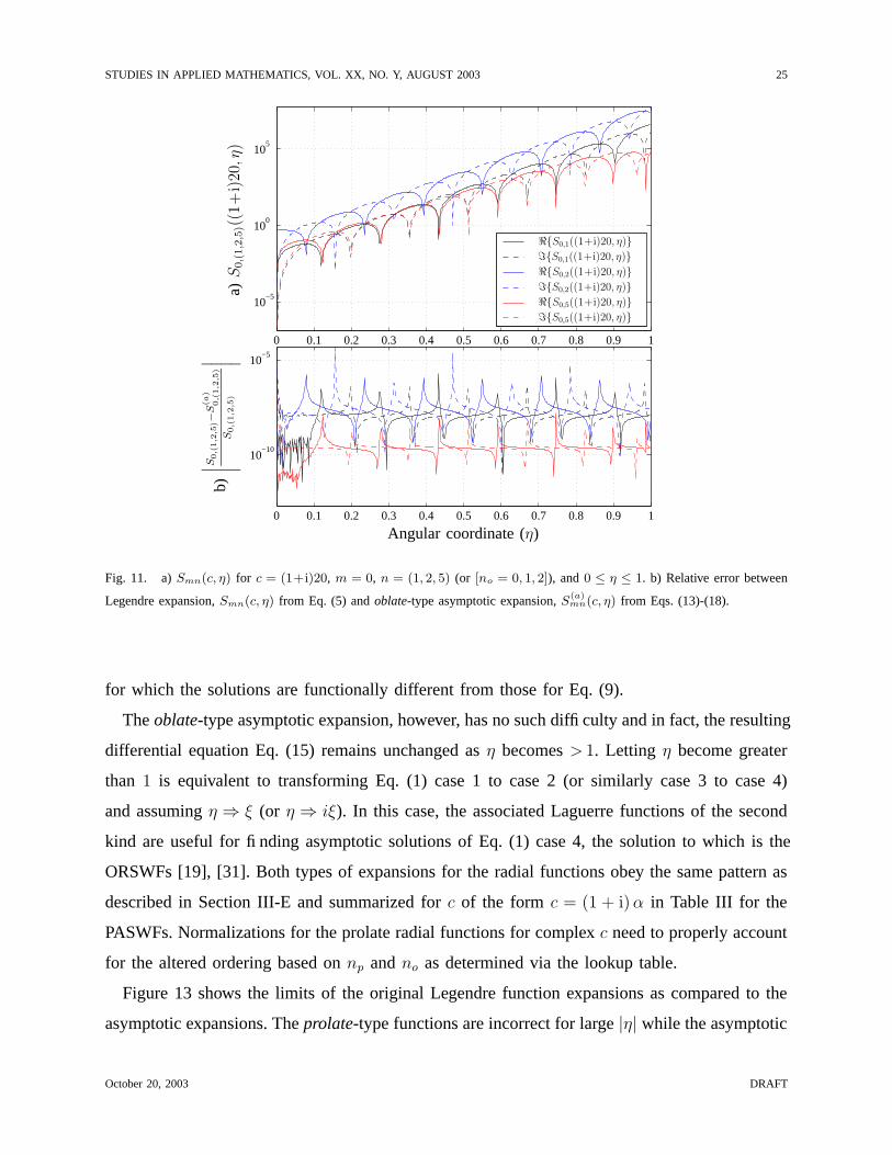
Some remarks about the behavior of these asymptotic expansions of the PASWFs for complex c

are in order. To begin with, the magnitudes of the oblate-type functions increase with increasing

|η|, whereas those functions approximated by prolate expansions [Eqs. (7)-(11)] decrease for

increasing |η|. S0,1(c, η), S0,2(c, η), and S0,5(c, η) for c = 20 + 20i and η = [0, 1] with their

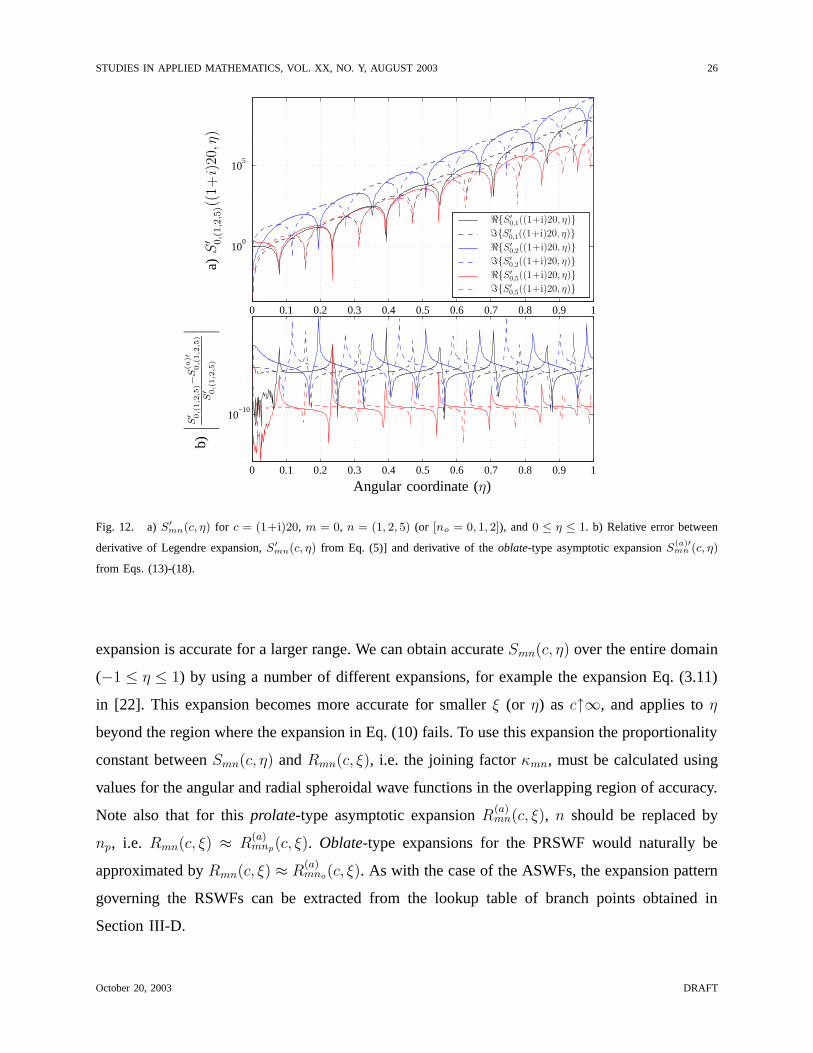
asymptotic expansions (all oblate-type) are shown in Fig. 11. Their first derivatives for the same

c are shown in Fig. 12. Furthermore, important differences are evident in the applicability of

the expansions in Section III to the case of η > 1, or in other words, to the PRSWF. For the case

of the prolate-type expansions, the continued presence of singularities at η = ±1, even under

transformation (Eq. (8)), causes increasing error as η approaches ±1. Letting η become greater

than 1 in Eq. (1) case 1 does not lead to Eq. (9), but leads instead to

d2umn

dx2+

(

−(

(n−m) +1

2

)

− x2

4

)

= 0, (39)



0 0.1 0.2 0.3 0.4 0.5 0.6 0.7 0.8 0.9 1

10−5

100

105

0 0.1 0.2 0.3 0.4 0.5 0.6 0.7 0.8 0.9 1

10−10

10−5

PSfrag replacements


a)S

0,(1,2

,5)(

(1+

i)20,η

)b)

∣ ∣ ∣ ∣

S0,(

1,2

,5)−

S(a

)0,(

1,2

,5)

S0,(

1,2

,5)

∣ ∣ ∣ ∣

<{S0,1((1+i)20, η)}={S0,1((1+i)20, η)}<{S0,2((1+i)20, η)}={S0,2((1+i)20, η)}<{S0,5((1+i)20, η)}={S0,5((1+i)20, η)}

Fig. 11. a) Smn(c, η) for c = (1+i)20, m = 0, n = (1, 2, 5) (or [no = 0, 1, 2]), and 0 ≤ η ≤ 1. b) Relative error between

Legendre expansion, Smn(c, η) from Eq. (5) and oblate-type asymptotic expansion, S(a)mn(c, η) from Eqs. (13)-(18).

for which the solutions are functionally different from those for Eq. (9).

The oblate-type asymptotic expansion, however, has no such difficulty and in fact, the resulting

differential equation Eq. (15) remains unchanged as η becomes > 1. Letting η become greater

than 1 is equivalent to transforming Eq. (1) case 1 to case 2 (or similarly case 3 to case 4)

and assuming η ⇒ ξ (or η ⇒ iξ). In this case, the associated Laguerre functions of the second

kind are useful for finding asymptotic solutions of Eq. (1) case 4, the solution to which is the

ORSWFs [19], [31]. Both types of expansions for the radial functions obey the same pattern as

described in Section III-E and summarized for c of the form c = (1 + i)α in Table III for the

PASWFs. Normalizations for the prolate radial functions for complex c need to properly account

for the altered ordering based on np and no as determined via the lookup table.

Figure 13 shows the limits of the original Legendre function expansions as compared to the

asymptotic expansions. The prolate-type functions are incorrect for large |η| while the asymptotic



0 0.1 0.2 0.3 0.4 0.5 0.6 0.7 0.8 0.9 1

100

105

0 0.1 0.2 0.3 0.4 0.5 0.6 0.7 0.8 0.9 1

10−10

PSfrag replacements


a)S′ 0,(1,2

,5)(

(1+i)

20,η

)b)

∣ ∣ ∣ ∣

S′ 0,(

1,2

,5)−

S(a

)′0,(

1,2

,5)

S′ 0,(

1,2

,5)

∣ ∣ ∣ ∣

<{S ′0,1((1+i)20, η)}

={S ′0,1((1+i)20, η)}

<{S ′0,2((1+i)20, η)}

={S ′0,2((1+i)20, η)}

<{S ′0,5((1+i)20, η)}

={S ′0,5((1+i)20, η)}

Fig. 12. a) S′

mn(c, η) for c = (1+i)20, m = 0, n = (1, 2, 5) (or [no = 0, 1, 2]), and 0 ≤ η ≤ 1. b) Relative error between

derivative of Legendre expansion, S ′

mn(c, η) from Eq. (5)] and derivative of the oblate-type asymptotic expansion S(a)′mn (c, η)

from Eqs. (13)-(18).

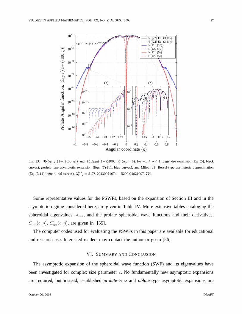
expansion is accurate for a larger range. We can obtain accurate Smn(c, η) over the entire domain

(−1 ≤ η ≤ 1) by using a number of different expansions, for example the expansion Eq. (3.11)

in [22]. This expansion becomes more accurate for smaller ξ (or η) as c↑∞, and applies to η

beyond the region where the expansion in Eq. (10) fails. To use this expansion the proportionality

constant between Smn(c, η) and Rmn(c, ξ), i.e. the joining factor κmn, must be calculated using

values for the angular and radial spheroidal wave functions in the overlapping region of accuracy.

Note also that for this prolate-type asymptotic expansion R(a)mn(c, ξ), n should be replaced by

np, i.e. Rmn(c, ξ) ≈ R(a)mnp(c, ξ). Oblate-type expansions for the PRSWF would naturally be

approximated by Rmn(c, ξ) ≈ R(a)mno(c, ξ). As with the case of the ASWFs, the expansion pattern

governing the RSWFs can be extracted from the lookup table of branch points obtained in

Section III-D.



−1 −0.8 −0.6 −0.4 −0.2 0 0.2 0.4 0.6 0.8 1

10−140

10−120

10−100

10−80

10−60

10−40

10−20

100

0 0.05 0.1 0.15 0.2

10−4

10−2

100

−0.75 −0.74 −0.73 −0.72 −0.7110

−52

10−50

10−48

10−46

10−44

PSfrag replacements

(a) (b)


Prol

ate

Ang

ular

func

tion,

|S0,(12((

1+i)

400,η)|

<{Eq. (5)}={Eq. (5)}

<{Eq. (10)}={Eq. (10)}

<{[22] Eq. (3.11)}={[22] Eq. (3.11)}

Fig. 13. <{S0,12((1+i)400, η)} and ={S0,12((1+i)400, η)} (np = 6), for −1 ≤ η ≤ 1. Legendre expansion (Eq. (5), black

curves), prolate-type asymptotic expansion (Eqs. (7)-(11, blue curves), and Miles [22] Bessel-type asymptotic approximation

(Eq. (3.11) therein, red curves). λ(a)0,12 = 5178.20430071674 + 5200.04621007177i.

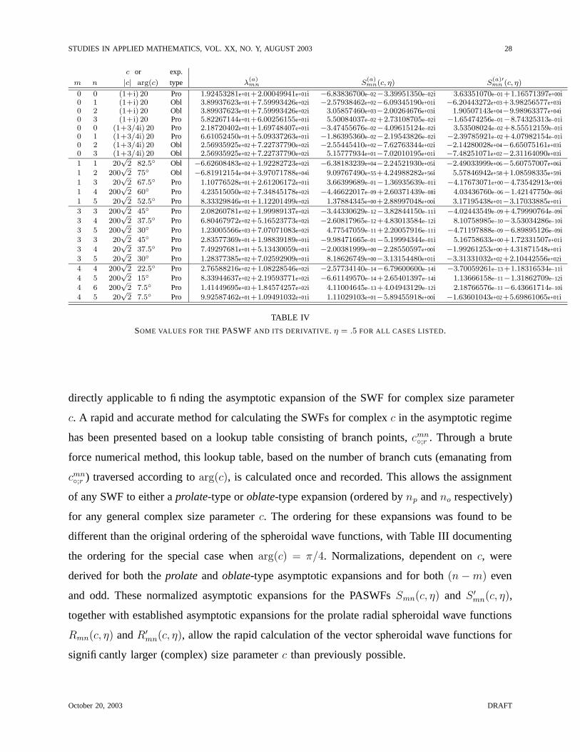
Some representative values for the PSWFs, based on the expansion of Section III and in the

asymptotic regime considered here, are given in Table IV. More extensive tables cataloging the

spheroidal eigenvalues, λmn, and the prolate spheroidal wave functions and their derivatives,

Smn(c, η), S ′mn(c, η), are given in [55].

The computer codes used for evaluating the PSWFs in this paper are available for educational

and research use. Interested readers may contact the author or go to [56].

VI. SUMMARY AND CONCLUSION

The asymptotic expansion of the spheroidal wave function (SWF) and its eigenvalues have

been investigated for complex size parameter c. No fundamentally new asymptotic expansions

are required, but instead, established prolate-type and oblate-type asymptotic expansions are



c or exp.

m n |c| arg(c) type λ(a)mn S

(a)mn(c, η) S

(a)′mn (c, η)

0 0 (1+i) 20 Pro 1.92453281e+01+2.00049941e+01i −6.83836700e–02−3.39951350e–02i 3.63351070e–01 +1.16571397e+00i0 1 (1+i) 20 Obl 3.89937623e+01+7.59993426e+02i −2.57938462e+02−6.09345190e+01i −6.20443272e+03+3.98256577e+03i0 2 (1+i) 20 Obl 3.89937623e+01+7.59993426e+02i 3.05857460e+03−2.00264676e+03i 1.90507143e+04−9.98963377e+04i0 3 (1+i) 20 Pro 5.82267144e+01+6.00256155e+01i 5.50084037e–02 +2.73108705e–02i −1.65474256e–01−8.74325313e–01i0 0 (1+3/4i) 20 Pro 2.18720402e+01+1.69748407e+01i −3.47455676e–02−4.09615124e–02i 3.53508024e–02 +8.55512159e–01i0 1 (1+3/4i) 20 Pro 6.61052450e+01+5.09337263e+01i −1.86395360e–02−2.19543826e–02i −2.39785921e–02 +4.07982154e–01i0 2 (1+3/4i) 20 Obl 2.56935925e+02+7.22737790e+02i −2.55445410e+02−7.62763344e+02i −2.14280028e+04−6.65075161e+03i0 3 (1+3/4i) 20 Obl 2.56935925e+02+7.22737790e+02i 5.15777934e+01−7.02010195e+01i −7.48251071e+02−2.31164090e+03i

1 1 20√

2 82.5◦ Obl −6.62608483e+02+1.92282723e+02i −6.38183239e+04−2.24521930e+05i −2.49033999e+06−5.60757007e+06i

1 2 200√

2 75◦ Obl −6.81912154e+04+3.97071788e+04i 9.09767490e+55+4.24988282e+56i 5.57846942e+58+1.08598335e+59i

1 3 20√

2 67.5◦ Pro 1.10776528e+01+2.61206172e+01i 3.66399689e–01−1.36935639e–01i −4.17673071e+00−4.73542913e+00i

1 4 200√

2 60◦ Pro 4.23515050e+02+7.34845178e+02i −4.46622017e–09 +2.60371439e–08i 4.03436760e–06−1.42147750e–06i

1 5 20√

2 52.5◦ Pro 8.33329846e+01+1.12201499e+02i 1.37884345e+00+2.88997048e+00i 3.17195438e+01−3.17033885e+01i

3 3 200√

2 45◦ Pro 2.08260781e+02+1.99989137e+02i −3.44330629e–12−3.82844150e–11i −4.02443549e–09 +4.79990764e–09i

3 4 200√

2 37.5◦ Pro 6.80467972e+02+5.16523773e+02i −2.60817965e–12 +4.83013584e–12i 8.10758985e–10−3.53034286e–10i

3 5 200√

2 30◦ Pro 1.23005566e+03+7.07071083e+02i 4.77547059e–11 +2.20057916e–11i −4.71197888e–09−6.89895126e–09i

3 3 20√

2 45◦ Pro 2.83577369e+01+1.98839189e+01i −9.98471665e–01−5.19994344e–01i 5.16758633e+00+1.72331507e+01i

3 4 20√

2 37.5◦ Pro 7.49297681e+01+5.13430059e+01i −2.00381999e+00−2.28550597e+00i −1.99261253e+00+4.31871548e+01i

3 5 20√

2 30◦ Pro 1.28377385e+02+7.02592909e+01i 8.18626749e+00−3.13154480e+01i −3.31331032e+02+2.10442556e+02i

4 4 200√

2 22.5◦ Pro 2.76588216e+02+1.08228546e+02i −2.57734140e–14−6.79600600e–14i −3.70059261e–13 +1.18316534e–11i

4 5 200√

2 15◦ Pro 8.33944637e+02+2.19593771e+02i −6.61149570e–14 +2.65401397e–14i 1.13666158e–11−1.31862709e–12i

4 6 200√

2 7.5◦ Pro 1.41449695e+03+1.84574257e+02i 4.11004645e–13 +4.04943129e–12i 2.18766576e–11−6.43661714e–10i

4 5 20√

2 7.5◦ Pro 9.92587462e+01+1.09491032e+01i 1.11029103e+01−5.89455918e+00i −1.63601043e+02+5.69861065e+01i

TABLE IV

SOME VALUES FOR THE PASWF AND ITS DERIVATIVE. η = .5 FOR ALL CASES LISTED.

directly applicable to finding the asymptotic expansion of the SWF for complex size parameter

c. A rapid and accurate method for calculating the SWFs for complex c in the asymptotic regime

has been presented based on a lookup table consisting of branch points, cmn◦;r . Through a brute

force numerical method, this lookup table, based on the number of branch cuts (emanating from

cmn◦;r ) traversed according to arg(c), is calculated once and recorded. This allows the assignment

of any SWF to either a prolate-type or oblate-type expansion (ordered by np and no respectively)

for any general complex size parameter c. The ordering for these expansions was found to be

different than the original ordering of the spheroidal wave functions, with Table III documenting

the ordering for the special case when arg(c) = π/4. Normalizations, dependent on c, were

derived for both the prolate and oblate-type asymptotic expansions and for both (n−m) even

and odd. These normalized asymptotic expansions for the PASWFs Smn(c, η) and S ′mn(c, η),

together with established asymptotic expansions for the prolate radial spheroidal wave functions

Rmn(c, η) and R′mn(c, η), allow the rapid calculation of the vector spheroidal wave functions for

significantly larger (complex) size parameter c than previously possible.



REFERENCES

[1] S. Asano and G. Yamamoto, “Light scattering by a spheroidal particle,” Appl. Opt., vol. 14, pp. 29–49, Jan. 1975.

[2] N. V. Voshchinnikov and V. G. Farafonov, “Optical properties of spheroidal particles,” Astrophys. Space Sci., vol. 204, pp.

19–86, June 1993.

[3] M. I. Mishchenko, J. W. Hovenier, and L. D. Travis, Eds., Light scattering by nonspherical particles: theory, measurements,

and applications. Academic Press, 2000.

[4] B. D. B. Figueiredo, “On some solutions to generalized spheroidal wave equations and applications,” Journal of Physics

A, vol. 35, no. 12, pp. 2877–906, March 2002.

[5] R. Chapman, “Digital filtering and higher order statistics,” IEE-Colloquium-on-Digital-Filters, pp. 4/1–4/6, April 1998.

[6] C. L. Fancourt and J. C. Principe, “On the relationship between the Karhunen-Loeve transform and the prolate spheroidal

wave functions,” ser. Proceedings IEEE ICASSP, vol. 1, 2000, pp. 261–4.

[7] F. Grunbaum and L. Miranian, “The magic of the prolate spheroidal functions in various setups,” Proc. SPIE, pp. 151–62,

2001.

[8] B. Larsson, T. Levitina, and E. J. Brandas, “On prolate spheroidal wave functions for signal processing,” International

Journal of Quantum Chemistry, vol. 85, no. 4-5, pp. 392–7, 2001.

[9] L. J. Chu and J. A. Stratton, “Forced oscillations of a prolate spheroid,” Journal of Applied Physics, vol. 12, pp. 241–248,

1941.

[10] M. F. R. Cooray, I. R. Ciric, and B. P. Sinha, “Electromagnetic scattering by a system of two parallel dielectric prolate

spheroids,” Canadian Journal of Physics, vol. 68, no. 4-5, pp. 376–84, 1990.

[11] M. F. R. Cooray and I. R. Ciric, “Scattering by systems of spheroids in arbitrary configurations,” Comp. Phys. Comm.,

vol. 68, pp. 279–305, 1991.

[12] R. S. Chen, E. K. N. Yung, D. G. Fang, and Z. M. Xie, “An efficient analysis of radiation from slotted coaxial cable using

the spheroidal wave function,” Microwave Opt. Technol. Lett., vol. 21, no. 5, pp. 372–7, 1999.

[13] L. W. Li, M. S. Leong, P. S. Kooi, and T. S. Yeo, “Spheroidal vector wave eigenfunction expansion of dyadic Green’s

functions for a dielectric spheroid,” IEEE Trans. on Antennas and Propagation, vol. 49, no. 4, pp. 645–59, April 2001.

[14] B. E. Barrowes, C. O. Ao, F. L. Teixeira, J. A. Kong, and L. Tsang, “Monte Carlo simulation of electromagnetic wave

propagation in dense random media with dielectric spheroids,” IEICE Trans. on Electronics, vol. E83-C, no. 12, pp.

1797–1802, December 2000.

[15] H. Braunisch, C. O. Ao, K. O’Neill, and J. A. Kong, “Magnetoquasistatic response of conducting and permeable spheroid

under axial excitation,” IEEE Trans. on Geoscience and Remote Sensing, vol. 39, no. 12, pp. 2689–2701, December 2001.

[16] C. O. Ao, H. Braunisch, K. O’Neill, , and J. A. Kong, “Quasi-magnetostatic solution for a conducting and permeable

spheroid with arbitrary excitation,” IEEE Trans. on Geoscience and Remote Sensing, vol. 40, no. 4, pp. 887–97, April

2002.

[17] J. A. Stratton, P. M. Morse, L. J. Chu, J. D. C. Little, and F. J. Corbato, Spheroidal Wave Functions. New York: John

Wiley and Sons, 1956.

[18] J. Meixner and F. W. Schafke, Mathieusche Funktionen und Spharoidfunktionen. Berlin: Springer-Verlag, 1954.

[19] C. Flammer, Spheroidal Wave Functions. Stanford: Stanford University Press, 1957.

[20] Tables of angular spheroidal wave functions. Washington: Naval Research Laboratory, 1975.

[21] D. Slepian, “Some asymptotic expansions for prolate spheroidal functions,” Journal of Math. and Physics, vol. 44, pp.

99–140, 1965.



[22] J. W. Miles, “Asymptotic approximations for prolate spheroidal wave functions,” Studies in Applied Mathematics, vol. 54,

no. 4, pp. 315–49, Dec. 1975.

[23] ——, “Asymptotic approximations for oblate spheroidal wave functions,” Phillips Research Reports, vol. 30, pp. 140–160,

1975.

[24] W. Streifer, “Uniform asymptotic expansions for prolate spheroidal wave functions,” Journal of Math. and Physics, vol. 47,

pp. 407–415, 1968.

[25] J. des Cloizeaux and M. L. Mehta, “Some asymptotic expressions for prolate spheroidal functions and for the eigenvalues of

differential and integral equations of which they are solutions,” Journal of Mathematical Physics, vol. 13, pp. 1745–1754,

1972.

[26] M. L. Sink and B. C. Eu, “A uniform WKB approximation for spheroidal wave functions,” Journal of Chemical Physics,

vol. 78, no. 8, pp. 4887–95, Apr. 1983.

[27] S. G. Volotovskii, N. L. Kazanskii, and S. N. Khonina, “Analysis and development of the methods for calculating eigenvalues

of prolate spheroidal wave functions of zero order,” Pattern Recognition and Image Analysis, vol. 11, no. 3, pp. 633–48,

2001.

[28] L. G. Guimaraes, “Explicit asymptotic formulae for the spheroidal angular eigenvalues,” Journal of Physics A, vol. 28,

no. 8, pp. L233–L237, 1995.

[29] P. C. G. de Moraes and L. G. Guimaraes, “Uniform asymptotic formulae for the spheroidal angular function,” Journal of

Quantitative Spectroscopy and Radiative Transfer, vol. 74, no. 6, pp. 757–65, Sep. 2002.

[30] T. Do-Nhat, “Asymptotic expansion of the Mathieu and prolate spheroidal eigenvalues for large parameter c,” Canadian

Journal of Physics, vol. 77, no. 8, pp. 635–652, aug 1999.

[31] ——, “Asymptotic expansions of the oblate spheroidal eigenvalues and wave functions for large parameter c,” Canadian

Journal of Physics, vol. 79, no. 5, pp. 813–31, May 2001.

[32] S. Asano and M. Sato, “Light scattering by randomly oriented spheroidal particles,” Applied Optics, vol. 19, no. 6, pp.

962–74, March 1980.

[33] R. J. Lytle and F. V. Schultz, “Prolate spheroidal antennas in isotropic plasma media,” IEEE Trans. on Antennas and

Propagation, vol. 17, no. 4, pp. 496–506, July 1969.

[34] F. W. Schafke and H. Groh, “Zur Berechnung der Eigenwerte der Spharoiddifferentialgleichung. (German) [On the

calculation of the eigenvalues of the spheroidal differential equation],” Numerical Mathematics, vol. 4, pp. 310–312,

1962.

[35] J. Meixner, F. W. Schafke, and W. Gerhard, Mathieu functions and spheroidal functions and their mathematical foundations,

further studies, ser. Lecture notes in mathematics. Berlin; New York: Springer-Verlag, 1980, no. 837.

[36] B. G. C. Hunter, “The eigenvalues of the angular spheroidal wave-equation,” Studies in Applied Mathematics, vol. 66,

no. 3, pp. 217–240, 1982.

[37] T. Oguchi, “Eigenvalues of spheroidal wave functions and their branch points for complex values of propagation constants,”

Radio Science, vol. 5, no. 8-9, pp. 1207–14, Aug. 1970.

[38] P. E. Falloon, P. C. Abbott, and J. B. Wang, “Theory and computation of spheroidal wavefunctions,” Journal of Physics

A, vol. 36, pp. 5477–5495, 2003.

[39] L.-W. Li, M. S. Leong, T. S. Yeo, P. S. Kooi, and K. Y. Tan, “Computations of spheroidal harmonics with complex argu-

ments: A review with an algorithm,” Physical Review E: Statistical Physics, Plasmas, Fluids, and Related Interdisciplinary

Topics, vol. 58, no. 5, pp. 6792–806, Nov. 1998.



[40] G. Lame, “(Liouville),” J. Math., vol. 2, no. 147, 1837.

[41] C. Niven, “On the conduction of heat in ellipsoids of revolution,” Philisophical Transactions of the Royal Society of

London, vol. 171, pp. 117–151, 1880.

[42] M. Abramowitz and I. A. Stegun, Handbook of Mathematical Functions, 9th ed. Dover Publications, Inc., 1970.

[43] C. J. Bouwkamp, “Theoretische en numerieke behandeling van de buiging door een ronde opening,” Ph.D. dissertation,

University of Groningen, Groningen, Netherlands, 1941.

[44] J. Caldwell, “Computation of eigenvalues of spheroidal harmonics using relaxation,” Journal of Physics A, vol. 21, pp.

3685–93, 1988.

[45] W. H. Press, B. P. Flannery, S. A. Teukolsky, and W. T. Vetterling, Numerical Recipes: The Art of Scientific Computing,

2nd ed. Cambridge (UK) and New York: Cambridge University Press, 1992.

[46] D. B. Hodge, “Eigenvalues and eigenfunctions of the spheroidal wave equation,” Journal of Mathematical Physics, vol. 11,

no. 8, pp. 2308–12, Aug. 1970.

[47] H. A. Eide, J. J. Stamnes, K. Stamnes, and F. M. Schulz, “New method for computing expansion coefficients for spheroidal

functions,” Journal of Quantitative Spectroscopy and Radiative Transfer, vol. 63, no. 2-6, pp. 191–203, Sept.–Dec. 1999.

[48] E. C. N. Aquino and E. Ley-Koo, “Spheroidal functions revisited: matrix evaluation and generating functions,” Revista

Mexicana de Fisica, vol. 48, no. 3, pp. 277–282, June 2002.

[49] B. E. Barrowes. (2002) MATLAB routines for computation of special functions. [Online]. Available: http:

//ceta.mit.edu/comp spec func/index.html

[50] S. Zhang and J. Jin, Computation of Special Functions. New York: John Wiley and Sons, 1996.

[51] A. Erdelyi, Ed., Higher transcendental functions, ser. Bateman Manuscript Project. New York: McGraw-Hill, 1953–55.

[52] C. M. Bender and S. A. Orszag, Advanced mathematical methods for scientists and engineers, ser. International series in

pure and applied mathematics. New York: McGraw-Hill, 1978.

[53] G. Strang, Introduction to Applied Mathematics. Wellesley-Cambridge Press, 1986.

[54] J. C. Lagarias, J. A. Reeds, M. H. Wright, and P. E. Wright, “Convergence properties of the nelder–mead simplex method

in low dimensions,” SIAM Journal on Optimization, vol. 9, no. 1, pp. 112–147, 1998.

[55] B. E. Barrowes, “Electromagnetic scattering and induction models for spheroidal geometries,” Ph.D. dissertation,

Massachusetts Institute of Technology, January 2004.

[56] ——. (2003) Center for electromagnetic theory and applications (CETA) website. [Online]. Available: http://ceta.mit.edu/


On the Asymptotic Expansion of the Spheroidal Wave ...barrowes/papers/barrowes_siam2003.pdf ·...

Documents

Transcript of On the Asymptotic Expansion of the Spheroidal Wave ...barrowes/papers/barrowes_siam2003.pdf ·...