ASYMPTOTIC CONDITIONAL PROBABILITIES: THE UNARY CASE · ASYMPTOTIC CONDITIONAL PROBABILITIES: THE...
55
ASYMPTOTIC CONDITIONAL PROBABILITIES: THE UNARY CASE * ADAM J. GROVE † , JOSEPH Y. HALPERN ‡ , AND DAPHNE KOLLER § Abstract. Motivated by problems that arise in computing degrees of belief, we consider the problem of computing asymptotic conditional probabilities for first-order sentences. Given first- order sentences ϕ and θ, we consider the structures with domain {1,...,N } that satisfy θ, and compute the fraction of them in which ϕ is true. We then consider what happens to this fraction as N gets large. This extends the work on 0-1 laws that considers the limiting probability of first- order sentences, by considering asymptotic conditional probabilities. As shown by L¯ ıogon’k¯ ı˘ ı[Math. Notes Acad. USSR, 6 (1969), pp. 856–861] and by Grove, Halpern, and Koller [Res. Rep. RJ 9564, IBM Almaden Research Center, San Jose, CA, 1993], in the general case, asymptotic conditional probabilities do not always exist, and most questions relating to this issue are highly undecidable. These results, however, all depend on the assumption that θ can use a nonunary predicate symbol. L¯ ıogon’k¯ ı˘ ı[Math. Notes Acad. USSR, 6 (1969), pp. 856–861] shows that if we condition on formulas θ involving unary predicate symbols only (but no equality or constant symbols), then the asymptotic conditional probability does exist and can be effectively computed. This is the case even if we place no corresponding restrictions on ϕ. We extend this result here to the case where θ involves equality and constants. We show that the complexity of computing the limit depends on various factors, such as the depth of quantifier nesting, or whether the vocabulary is finite or infinite. We completely characterize the complexity of the problem in the different cases, and show related results for the associated approximation problem. Key words. asymptotic probability, 0-1 law, finite model theory, degree of belief, labeled structures, principle of indifference, complexity AMS subject classifications. 03B48, 60C05, 68Q25 1. Introduction. Suppose we have a sentence θ expressing facts that are known to be true, and another sentence ϕ whose truth is uncertain. Our knowledge θ is often insufficient to determine the truth of ϕ: both ϕ and its negation may be consistent with θ. In such cases, it can be useful to assign a probability to ϕ given θ. In a companion paper [23], we described our motivation for investigating this idea, and presented our general approach. We repeat some of this material below, to provide the setting for the results of this paper. One important application of assigning probabilities to sentences—indeed, the one that has provided most of our motivation—is in the domain of decision theory and artificial intelligence. Consider an agent (or expert system) whose knowledge consists of some facts θ, who would like to assign a degree of belief to a particular statement ϕ. For example, a doctor may want to assign a degree of belief to the hypothesis that * Received by the editors October 13, 1993; accepted for publication (in revised form) July 7, 1994. Some of this research was performed while Adam Grove and Daphne Koller were at Stanford University and at the IBM Almaden Research Center. A preliminary version of this paper appeared in Proc. 24th ACM Symp. on Theory of Computing [20]. This research was sponsored in part by an IBM Graduate Fellowship to Adam Grove, by a University of California President’s Postdoctoral Fel- lowship to Daphne Koller, and by Air Force Office of Scientific Research contract F49620-91-C-0080. The United States Government is authorized to reproduce and distribute reprints for governmental purposes. Posted with permission from the SIAM Journal on Computing, Vol. 25, No. 1. Copyright 1996 by the Society for Industrial and Applied Mathematics. All rights reserved. † NEC Research Institute, 4 Independence Way, Princeton, NJ 08540 ([email protected]). ‡ IBM Almaden Research Center, 650 Harry Rd., San Jose, CA 95120 ([email protected]). § Computer Science Division, University of California at Berkeley, Berkeley, CA 94720 ([email protected]). 1
Transcript of ASYMPTOTIC CONDITIONAL PROBABILITIES: THE UNARY CASE · ASYMPTOTIC CONDITIONAL PROBABILITIES: THE...

ASYMPTOTIC CONDITIONAL PROBABILITIES: THE UNARYCASE∗
ADAM J. GROVE† , JOSEPH Y. HALPERN‡ , AND DAPHNE KOLLER§
Abstract. Motivated by problems that arise in computing degrees of belief, we consider theproblem of computing asymptotic conditional probabilities for first-order sentences. Given first-order sentences ϕ and θ, we consider the structures with domain 1, . . . , N that satisfy θ, andcompute the fraction of them in which ϕ is true. We then consider what happens to this fractionas N gets large. This extends the work on 0-1 laws that considers the limiting probability of first-order sentences, by considering asymptotic conditional probabilities. As shown by Lıogon’kı ı [Math.Notes Acad. USSR, 6 (1969), pp. 856–861] and by Grove, Halpern, and Koller [Res. Rep. RJ 9564,IBM Almaden Research Center, San Jose, CA, 1993], in the general case, asymptotic conditionalprobabilities do not always exist, and most questions relating to this issue are highly undecidable.These results, however, all depend on the assumption that θ can use a nonunary predicate symbol.Lıogon’kı ı [Math. Notes Acad. USSR, 6 (1969), pp. 856–861] shows that if we condition on formulasθ involving unary predicate symbols only (but no equality or constant symbols), then the asymptoticconditional probability does exist and can be effectively computed. This is the case even if we placeno corresponding restrictions on ϕ. We extend this result here to the case where θ involves equalityand constants. We show that the complexity of computing the limit depends on various factors, suchas the depth of quantifier nesting, or whether the vocabulary is finite or infinite. We completelycharacterize the complexity of the problem in the different cases, and show related results for theassociated approximation problem.
Key words. asymptotic probability, 0-1 law, finite model theory, degree of belief, labeledstructures, principle of indifference, complexity
AMS subject classifications. 03B48, 60C05, 68Q25
1. Introduction. Suppose we have a sentence θ expressing facts that are knownto be true, and another sentence ϕ whose truth is uncertain. Our knowledge θ is ofteninsufficient to determine the truth of ϕ: both ϕ and its negation may be consistentwith θ. In such cases, it can be useful to assign a probability to ϕ given θ. In acompanion paper [23], we described our motivation for investigating this idea, andpresented our general approach. We repeat some of this material below, to providethe setting for the results of this paper.
One important application of assigning probabilities to sentences—indeed, the onethat has provided most of our motivation—is in the domain of decision theory andartificial intelligence. Consider an agent (or expert system) whose knowledge consistsof some facts θ, who would like to assign a degree of belief to a particular statementϕ. For example, a doctor may want to assign a degree of belief to the hypothesis that
∗Received by the editors October 13, 1993; accepted for publication (in revised form) July 7,1994. Some of this research was performed while Adam Grove and Daphne Koller were at StanfordUniversity and at the IBM Almaden Research Center. A preliminary version of this paper appearedin Proc. 24th ACM Symp. on Theory of Computing [20]. This research was sponsored in part by anIBM Graduate Fellowship to Adam Grove, by a University of California President’s Postdoctoral Fel-lowship to Daphne Koller, and by Air Force Office of Scientific Research contract F49620-91-C-0080.The United States Government is authorized to reproduce and distribute reprints for governmentalpurposes. Posted with permission from the SIAM Journal on Computing, Vol. 25, No. 1. Copyright1996 by the Society for Industrial and Applied Mathematics. All rights reserved.
†NEC Research Institute, 4 Independence Way, Princeton, NJ 08540 ([email protected]).‡IBM Almaden Research Center, 650 Harry Rd., San Jose, CA 95120
([email protected]).§Computer Science Division, University of California at Berkeley, Berkeley, CA 94720
1

2 ADAM J. GROVE, JOSEPH Y. HALPERN, AND DAPHNE KOLLER
a patient has a particular illness, based on the symptoms exhibited by the patienttogether with general information about symptoms and diseases. Since the actionsthe agent takes may depend crucially on this value, we would like techniques forcomputing degrees of belief in a principled manner.
The difficulty of defining a principled technique for computing the probabilityof ϕ given θ, and then actually computing that probability, depends in part on thelanguage and logic being considered. In decision theory, applications often demand theability to express statistical knowledge (for instance, correlations between symptomsand diseases) as well as first-order knowledge. Work in the field of 0-1 laws (which, asdiscussed below, is closely related to our own) has examined some higher-order logicsas well as first-order logic. Nevertheless, the pure first-order case is still difficult, andis important because it provides a foundation for all extensions. In this paper and in[23] we address the problem of computing conditional probabilities in the first-ordercase. In a related paper [22], we consider the case of a first-order logic augmentedwith statistical knowledge.
The general problem of assigning probabilities to first-order sentences has beenwell studied (cf. [15] and [16]). In this paper, we investigate two specific formalisms forcomputing probabilities, based on the same basic approach. Our approach is itself aninstance of a much older idea, known as the principle of insufficient reason [28] or theprinciple of indifference [26]. This states that all possibilities should be given equalprobability, and was once regarded as one of the most basic principles of probabilitytheory. (See [24] for a discussion of the history of the principle.) We use this ideato assign equal degrees of belief to all basic “situations” consistent with the knownfacts. The two formalisms we consider differ only in how they interpret “situation.”We discuss this in more detail below.
In many applications, including the one of most interest to us, it makes sense toconsider finite domains only. In fact, the case of most interest to us is the behaviorof the formulas ϕ and θ over large finite domains. Similar questions also arise inthe area of 0-1 laws. Our approach essentially generalizes the methods used in thework on 0-1 laws for first-order logic to the case of conditional probabilities. (SeeCompton’s overview [8] for an introduction to this work.) Assume, without loss ofgenerality, that the domain is 1, . . . , N for some natural number N . As we saidabove, we consider two notions of “situation.” In the random-worlds method, the pos-sible situations are all the worlds, or first-order models, with domain 1, . . . , N thatsatisfy the constraints θ. Based on the principle of indifference, we assume that allworlds are equally likely. To assign a probability to ϕ, we therefore simply computethe fraction of them in which the sentence ϕ is true. The random-worlds approachviews each individual in 1, . . . , N as having a distinct name (even though the namemay not correspond to any constant in the vocabulary). Thus, two worlds that areisomorphic with respect to the symbols in the vocabulary are still treated as dis-tinct situations. In some cases, however, we may believe that all relevant distinctionsare captured by our vocabulary, and that isomorphic worlds are not truly distinct.The random-structures method attempts to capture this intuition by considering asituation to be a structure—an isomorphism class of worlds. This corresponds toassuming that individuals are distinguishable only if they differ with respect to prop-erties definable by the language. As before, we assign a probability to ϕ by comput-ing the fraction of the structures that satisfy ϕ among those structures that satisfyθ.1
1The random-worlds method considers what has been called in the literature labeled structures,

ASYMPTOTIC CONDITIONAL PROBABILITIES 3
Since we are computing probabilities over finite models, we have assumed thatthe domain is 1, . . . , N for some N . However, we often do not know the precisedomain size N . In many cases, we know only that N is large. We therefore estimatethe probability of ϕ given θ by the asymptotic limit, as N grows to infinity, of thisprobability over models of size N .
Precisely the same definitions of asymptotic probability are used in the context of0-1 laws for first-order logic, but without allowing prior information θ. The original0-1 law, proved independently by Glebskiı et al. [18] and Fagin [13], states that theasymptotic probability of any first-order sentence ϕ with no constant or functionsymbols is either 0 or 1. This means that such a sentence is true in almost all finitestructures, or in almost none.
Our work differs from the original work on 0-1 laws in two respects. The firstis relatively minor: we need to allow the use of constant symbols in ϕ, as they arenecessary when discussing individuals (such as patients). Although this is a minorchange, it is worth observing that it has a significant impact. It is easy to see that oncewe allow constant symbols, the asymptotic probability of a sentence ϕ is no longereither 0 or 1; for example, the asymptotic probability of P (c) is 1
2 . Moreover, once weallow constant symbols, the asymptotic probability under random worlds and underrandom structures need not be the same. The more significant difference, however, isthat we are interested in the asymptotic conditional probability of ϕ, given some priorknowledge θ. That is, we want the probability of ϕ over the class of finite structuresdefined by θ.
Some work has already been done on aspects of this question. Lıogon’kı ı [31],and independently Fagin [13], showed that asymptotic conditional probabilities donot necessarily converge to any limit. Subsequently, 0-1 laws were proved for specialclasses of first-order structures (such as graphs, tournaments, partial orders, etc.; seethe overview paper [8] for details and further references). In many cases, the classesconsidered could be defined in terms of first-order constraints. Thus, these resultscan be viewed as special cases of the problem that we are interested in: computingasymptotic conditional probabilities relative to structures satisfying the constraintsof a database. Lynch [32] showed that, for the random-worlds method, asymptoticprobabilities exist for first-order sentences involving unary functions, although thereis no 0-1 law. (Recall that the original 0-1 result is specifically for first-order logicwithout function symbols.) This can also be viewed as a special case of an asymptoticconditional probability for first-order logic without functions, since we can replacethe unary functions by binary predicates, and condition on the fact that they arefunctions.
The most comprehensive work on this problem is the work of Lıogon’kı ı [31].2
In addition to pointing out that asymptotic conditional probabilities do not existin general, he shows that it is undecidable whether such a probability exists. (Wegeneralize Lıogon’kı ı’s results for this case in [23].) He then investigates the specialcase of conditioning on formulas involving unary predicates only (but no constants
while the random-structures method considers unlabeled structures [8]. We choose to use our ownterminology for the random-worlds and random-structures methods, rather than the terminology oflabeled and unlabeled. This is partly because we feel it is more descriptive, and partly because thereare other variants of the approach that are useful for our intended application, and that do not fitinto the standard labeled/unlabeled structures dichotomy (see [2]).
2In an earlier version of this paper [21], we stated that, to our knowledge, no work had been doneon the general problem of asymptotic conditional probabilities. We thank Moshe Vardi for pointingout to us the work of Lıogon’kı ı [31].
4 ADAM J. GROVE, JOSEPH Y. HALPERN, AND DAPHNE KOLLER
or equality). In this case, he proves that the asymptotic conditional probability doesexist and can be effectively computed, even if the left side of the conditional, ϕ, haspredicates of arbitrary arity and equality. This gap between unary predicates andbinary predicates is somewhat reminiscent of the fact that first-order logic over avocabulary with only unary predicates (and constant symbols) is decidable, while ifwe allow even a single binary predicate symbol, then it becomes undecidable [11],[29]. This similarity is not coincidental; some of the techniques used to show thatfirst-order logic over a vocabulary with unary predicate symbols is decidable are usedby us to show that asymptotic conditional probabilities exist.
In this paper, we extend the results of Lıogon’kı ı [31] for the unary case. Wefirst prove (in §3) that, if we condition on a formula involving only unary predicates,constants, and equality that is satisfiable in arbitrarily large models, the asymptoticconditional probability exists. We also present an algorithm for computing this limit.The main idea we use is the following: to compute the asymptotic conditional prob-ability of ϕ given θ, we examine the behavior of ϕ in finite models of θ. It turns outthat we can partition the models of θ into a finite collection of classes, such that ϕbehaves uniformly in any individual class. By this we mean that almost all worldsin the class satisfy ϕ or almost none do; i.e., there is a 0-1 law for the asymptoticprobability of ϕ when we restrict attention to models in a single class. In §3 we definethese classes and prove the existence of a 0-1 law within each class. We also showhow the asymptotic conditional probability of ϕ given θ can be computed using these0-1 probabilities.
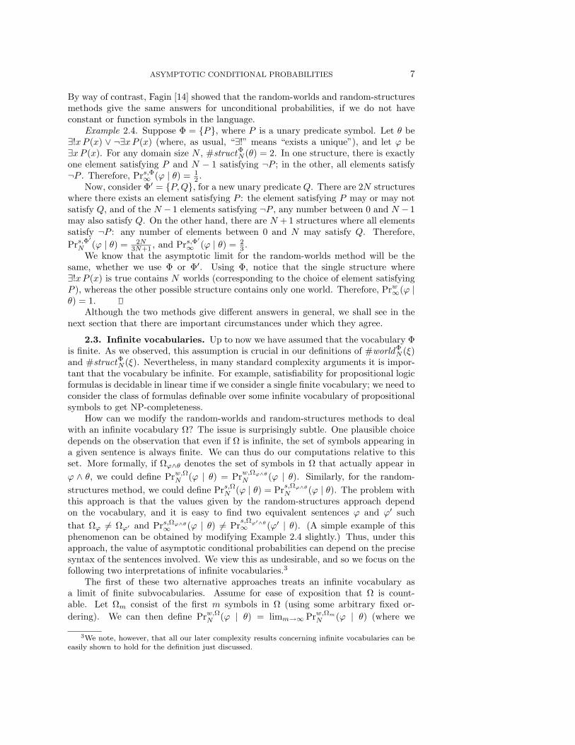
In §4 we turn our attention to the complexity of computing the asymptotic prob-ability in this case. Our results, which are the same for random worlds and randomstructures, depend on several factors: whether the vocabulary is finite or infinite,whether there is a bound on the depth of quantifier nesting, whether equality is usedin θ, whether nonunary predicates are used, and whether there is a bound on pred-icate arities. For a fixed and finite vocabulary, there are just two cases: if there isno bound on the depth of quantifier nesting then computing asymptotic conditionalprobabilities is PSPACE-complete, otherwise the computation can be done in lineartime. The case in which the vocabulary is not fixed (which is the case more typicallyconsidered in complexity theory) is more complex. The results for this case are sum-marized in Table 1.1. Perhaps the most interesting aspect of this table is the factorsthat cause the difference in complexity between #EXP and #TA(EXP,LIN) (where#TA(EXP,LIN) is the counting class corresponding to alternating Turing machinesthat take exponential time and make only a linear number of alternations; a formaldefinition is provided in §4.5). If we allow the use of equality in θ, then we need torestrict both ϕ and θ to using only unary predicates to get the #EXP upper bound.On the other hand, if θ does not mention equality, then the #EXP upper bound isattained as long as there is some fixed bound on the arity of the predicates appearingin ϕ. If we have no bound on the arity of the predicates that appear in ϕ, or if weallow equality in θ and predicates of arity 2 in ϕ, then the #EXP upper bound nolonger holds, and we move to #TA(EXP,LIN).
Our results showing that computing the asymptotic probability is hard can beextended to show that finding a nontrivial estimate of the probability (i.e., decidingif it lies in a nontrivial interval) is almost as difficult. The lower bounds for thearity-bounded case and the general case require formulas of quantification depth 2 ormore. For unquantified sentences or depth-1 quantification, things seem to becomean exponential factor easier. We do not have tight bounds for the complexity of

ASYMPTOTIC CONDITIONAL PROBABILITIES 5
Table 1.1Complexity of asymptotic conditional probabilities.
Depth ≤ 1 Restricted General caseExistence NP-complete NEXPTIME-complete NEXPTIME-completeCompute #P/PSPACE #EXP-complete #TA(EXP,LIN)-completeApproximate (co-)NP-hard (co-)NEXPTIME-hard TA(EXP,LIN)-hard
computing the degree of belief in this case; we have a #P lower bound and a PSPACEupper bound. The results for depth 1 are not proved in this paper; see [27] for details.
We observe that apart from our precise classification of the complexity of theseproblems, our analysis provides an effective algorithm for computing the asymptoticconditional probability. The complexity of this algorithm is, in general, double-exponential in the number of unary predicates used and in the maximum arity ofany predicate symbol used; it is exponential in the overall size of the vocabulary andin the lengths of ϕ and θ.
Our results are of more than purely technical interest. The random-worlds methodis of considerable theoretical and practical importance. We have already mentioned itsrelevance to computing degrees of belief. There are well-known results from physicsthat show the close connection between the random-worlds method and maximumentropy [25]. These results say that in certain cases the asymptotic probability canbe computed using maximum entropy methods. Some formalization of similar results,but in a framework that is close to that of the current paper, can be found in [33]and [22]. (These results are of far more interest when there are statistical assertionsin the language, so we do not discuss them here.)
As we observe in [23] and [22], this connection relies on the fact that we areconditioning on a unary formula. In fact, in almost all applications where maximumentropy has been used (and where its application can be best justified in terms ofthe random-worlds method) the knowledge base is described in terms of unary pred-icates (or, equivalently, unary functions with a finite range). For example, in physicsapplications we are interested in such predicates as quantum state (see [10]). Simi-larly, AI applications and expert systems typically use only unary predicates [7] suchas symptoms and diseases. In general, many properties of interest can be expressedusing unary predicates, since they express properties of individuals. Indeed, a goodcase can be made that statisticians tend to reformulate all problems in terms of unarypredicates, since an event in a sample space can be identified with a unary predicate[36]. Indeed, in most cases where statistics are used, we have a basic unit in mind (anindividual, a family, a household, etc.), and the properties (predicates) we considerare typically relative to a single unit (i.e., unary predicates). Thus, results concerningcomputing the asymptotic conditional probability if we condition on unary formulasare significant in practice.
2. Definitions. Let Φ be a set of predicate and function symbols, and let L(Φ)(resp., L−(Φ)) denote the set of first-order sentences over Φ with equality (resp.,without equality). To simplify the presentation, we begin by assuming that Φ isfinite; the case of an infinite vocabulary is deferred to §2.3. Much of the material in§§2.1 and 2.2 is taken from [23].
2.1. The random-worlds method. We begin by defining the random-worlds,or labeled, method. Given a sentence ξ ∈ L(Φ), let #worldΦ
N (ξ) be the number ofworlds, or first-order models, of ξ over Φ with domain 1, . . . , N. Note that the

6 ADAM J. GROVE, JOSEPH Y. HALPERN, AND DAPHNE KOLLER
assumption that Φ is finite is necessary for #worldΦN (ξ) to be well defined. Define
Prw,ΦN (ϕ | θ) =#worldΦ
N (ϕ ∧ θ)#worldΦ
N (θ).
In [23], we proved the following proposition.Proposition 2.1. Let Φ,Φ′ be finite vocabularies, and let ϕ, θ be sentences in
both L(Φ) and L(Φ′). Then Prw,ΦN (ϕ | θ) = Prw,Φ′
N (ϕ | θ).Thus, the value of Prw,ΦN (ϕ | θ) does not depend on the choice of Φ. We therefore
omit reference to Φ in Prw,ΦN (ϕ | θ), writing PrwN (ϕ | θ) instead.We would like to define Prw∞(ϕ | θ) as the limit limN→∞ PrwN (ϕ | θ). There is
a small technical problem we have to deal with in this definition: we must decidewhat to do if #worldΦ
N (θ) = 0, so that PrwN (ϕ | θ) is not well defined. In [23], wedifferentiate between the case where PrwN (ϕ | θ) is well defined for all but finitely manyN ’s, and the case where it is well defined for infinitely many N ’s. As we shall show(see Lemma 3.30) this distinction need not be made when θ is a unary formula. Thus,for the purposes of this paper, we use the following definition of well-definedness,which is simpler than that of [23].
Definition 2.2. The asymptotic conditional probability according to the random-worlds method, denoted Prw∞(ϕ | θ), is well defined if #worldΦ
N (θ) 6= 0 for all butfinitely many N . If Prw∞(ϕ | θ) is well defined, then we take Prw∞(ϕ | θ) to denotelimN→∞ PrwN (ϕ | θ).
Note that for any formula ϕ, the issue of whether Prw∞(ϕ | θ) is well defined iscompletely determined by θ. Therefore, when investigating the question of how todecide whether such a probability is well defined, it is often useful to ignore ϕ. Wetherefore say that Prw∞(∗ | θ) is well defined if Prw∞(ϕ | θ) is well defined for everyformula ϕ (which is true iff Prw∞(true | θ) is well defined).
2.2. The random-structures method. As we explained in the introduction,the random-structures method is motivated by the intuition that worlds that areindistinguishable within the language should only be counted once. Thus, the random-structures method counts the number of (unlabeled ) structures, or isomorphism classesof worlds.
Formally, we proceed as follows. Given a sentence ξ ∈ L(Φ), let #structΦN (ξ)
be the number of isomorphism classes of worlds with domain 1, . . . , N over thevocabulary Φ satisfying ξ. Note that since all the worlds that make up a structureagree on the truth value they assign to ξ, it makes sense to talk about a structuresatisfying or not satisfying ξ. We can then proceed, as before, to define Prs,ΦN (ϕ | θ)as #structΦN (ϕ∧θ)
#structΦN
(θ). We define asymptotic conditional probability, denoted Prs,Φ∞ (ϕ | θ)
in terms of Prs,ΦN (ϕ | θ), in analogy to the earlier definition for random worlds. It isclear that #worldΦ
N (θ) = 0 iff #structΦN (θ) = 0, so that well-definedness is equivalent
for the two methods, for any ϕ, θ.Proposition 2.3. For any θ ∈ L(Φ), Prw∞(∗ | θ) is well defined iff Prs,Φ∞ (∗ | θ)
is well defined.As the following example, taken from [23], shows, for the random-structures
method the analogue to Proposition 2.1 does not hold; the value of Prs,ΦN (ϕ | θ), andeven the value of the limit, depends on the choice of Φ. This example, together withProposition 2.1, also demonstrates that the values of conditional probabilities gen-erally differ between the random-worlds method and the random-structures method.
ASYMPTOTIC CONDITIONAL PROBABILITIES 7
By way of contrast, Fagin [14] showed that the random-worlds and random-structuresmethods give the same answers for unconditional probabilities, if we do not haveconstant or function symbols in the language.
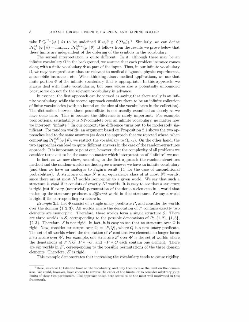
Example 2.4. Suppose Φ = P, where P is a unary predicate symbol. Let θ be∃!xP (x) ∨ ¬∃xP (x) (where, as usual, “∃!” means “exists a unique”), and let ϕ be∃xP (x). For any domain size N , #structΦ
N (θ) = 2. In one structure, there is exactlyone element satisfying P and N − 1 satisfying ¬P ; in the other, all elements satisfy¬P . Therefore, Prs,Φ∞ (ϕ | θ) = 1
2 .Now, consider Φ′ = P,Q, for a new unary predicate Q. There are 2N structures
where there exists an element satisfying P : the element satisfying P may or may notsatisfy Q, and of the N − 1 elements satisfying ¬P , any number between 0 and N − 1may also satisfy Q. On the other hand, there are N + 1 structures where all elementssatisfy ¬P : any number of elements between 0 and N may satisfy Q. Therefore,Prs,Φ
′
N (ϕ | θ) = 2N3N+1 , and Prs,Φ
′
∞ (ϕ | θ) = 23 .
We know that the asymptotic limit for the random-worlds method will be thesame, whether we use Φ or Φ′. Using Φ, notice that the single structure where∃!xP (x) is true contains N worlds (corresponding to the choice of element satisfyingP ), whereas the other possible structure contains only one world. Therefore, Prw∞(ϕ |θ) = 1.
Although the two methods give different answers in general, we shall see in thenext section that there are important circumstances under which they agree.
2.3. Infinite vocabularies. Up to now we have assumed that the vocabulary Φis finite. As we observed, this assumption is crucial in our definitions of #worldΦ
N (ξ)and #structΦ
N (ξ). Nevertheless, in many standard complexity arguments it is impor-tant that the vocabulary be infinite. For example, satisfiability for propositional logicformulas is decidable in linear time if we consider a single finite vocabulary; we need toconsider the class of formulas definable over some infinite vocabulary of propositionalsymbols to get NP-completeness.
How can we modify the random-worlds and random-structures methods to dealwith an infinite vocabulary Ω? The issue is surprisingly subtle. One plausible choicedepends on the observation that even if Ω is infinite, the set of symbols appearing ina given sentence is always finite. We can thus do our computations relative to thisset. More formally, if Ωϕ∧θ denotes the set of symbols in Ω that actually appear inϕ ∧ θ, we could define Prw,ΩN (ϕ | θ) = Prw,Ωϕ∧θN (ϕ | θ). Similarly, for the random-structures method, we could define Prs,ΩN (ϕ | θ) = Prs,Ωϕ∧θN (ϕ | θ). The problem withthis approach is that the values given by the random-structures approach dependon the vocabulary, and it is easy to find two equivalent sentences ϕ and ϕ′ suchthat Ωϕ 6= Ωϕ′ and Prs,Ωϕ∧θ∞ (ϕ | θ) 6= Pr
s,Ωϕ′∧θ∞ (ϕ′ | θ). (A simple example of this
phenomenon can be obtained by modifying Example 2.4 slightly.) Thus, under thisapproach, the value of asymptotic conditional probabilities can depend on the precisesyntax of the sentences involved. We view this as undesirable, and so we focus on thefollowing two interpretations of infinite vocabularies.3
The first of these two alternative approaches treats an infinite vocabulary asa limit of finite subvocabularies. Assume for ease of exposition that Ω is count-able. Let Ωm consist of the first m symbols in Ω (using some arbitrary fixed or-dering). We can then define Prw,ΩN (ϕ | θ) = limm→∞ Prw,ΩmN (ϕ | θ) (where we
3We note, however, that all our later complexity results concerning infinite vocabularies can beeasily shown to hold for the definition just discussed.
8 ADAM J. GROVE, JOSEPH Y. HALPERN, AND DAPHNE KOLLER
take Prw,ΩmN (ϕ | θ) to be undefined if ϕ, θ /∈ L(Ωm)).4 Similarly, we can definePrs,ΩN (ϕ | θ) = limm→∞ Prs,ΩmN (ϕ | θ). It follows from the results we prove below thatthese limits are independent of the ordering of the symbols in the vocabulary.
The second interpretation is quite different. In it, although there may be aninfinite vocabulary Ω in the background, we assume that each problem instance comesalong with a finite vocabulary Φ as part of the input. Thus, in our infinite vocabularyΩ, we may have predicates that are relevant to medical diagnosis, physics experiments,automobile insurance, etc. When thinking about medical applications, we use thatfinite portion Φ of the infinite vocabulary that is appropriate. In this approach, wealways deal with finite vocabularies, but ones whose size is potentially unboundedbecause we do not fix the relevant vocabulary in advance.
In essence, the first approach can be viewed as saying that there really is an infi-nite vocabulary, while the second approach considers there to be an infinite collectionof finite vocabularies (with no bound on the size of the vocabularies in the collection).The distinction between these possibilities is not usually examined as closely as wehave done here. This is because the difference is rarely important. For example,propositional satisfiability is NP-complete over an infinite vocabulary, no matter howwe interpret “infinite.” In our context, the difference turns out to be moderately sig-nificant. For random worlds, an argument based on Proposition 2.1 shows the two ap-proaches lead to the same answers (as does the approach that we rejected where, whencomputing Prw,ΩN (ϕ | θ), we restrict the vocabulary to Ωϕ∧θ). On the other hand, thetwo approaches can lead to quite different answers in the case of the random-structuresapproach. It is important to point out, however, that the complexity of all problems weconsider turns out to be the same no matter which interpretation of “infinite” we use.
In fact, as we now show, according to the first approach the random-structuresmethod and the random-worlds method agree whenever we have an infinite vocabulary(and thus we have an analogue to Fagin’s result [14] for the case of unconditionalprobabilities). A structure of size N is an equivalence class of at most N ! worlds,since there are at most N ! worlds isomorphic to a given world. We say that such astructure is rigid if it consists of exactly N ! worlds. It is easy to see that a structureis rigid just if every (nontrivial) permutation of the domain elements in a world thatmakes up the structure produces a different world in that structure. We say a worldis rigid if the corresponding structure is.
Example 2.5. Let Φ consist of a single unary predicate P , and consider the worldsover the domain 1, 2, 3. All worlds where the denotation of P contains exactly twoelements are isomorphic. Therefore, these worlds form a single structure S. Thereare three worlds in S, corresponding to the possible denotations of P : 1, 2, 1, 3,2, 3. Therefore, S is not rigid. In fact, it is easy to see that no structure over Φ isrigid. Now, consider structures over Φ′ = P,Q, where Q is a new unary predicate.The set of all worlds where the denotation of P contains two elements no longer formsa structure over Φ′. For example, one structure S ′ over Φ′ is the set of worlds wherethe denotations of P ∧ Q, P ∧ ¬Q, and ¬P ∧ Q each contain one element. Thereare six worlds in S ′, corresponding to the possible permutations of the three domainelements. Therefore, S ′ is rigid.
This example demonstrates that increasing the vocabulary tends to cause rigidity.
4Here, we chose to take the limit on the vocabulary, and only then to take the limit on the domainsize. We could, however, have chosen to reverse the order of the limits, or to consider arbitrary jointlimits of these two parameters. The approach taken here seems to be the most well motivated in thisframework.

ASYMPTOTIC CONDITIONAL PROBABILITIES 9
We now formalize this intuition, and show its importance. Note that in the followingdefinition (and throughout the paper) all logarithms are taken to the base 2.
Definition 2.6. We say that a vocabulary Φ is sufficiently rich with respect toN if
(a) Φ contains at least κN constant symbols and κN ≥ N2 logN , or(b) Φ contains at least πN unary predicate symbols and πN ≥ 3 logN , or(c) Φ contains at least one nonunary predicate symbol.Fagin showed that if Φ contains at least one nonunary predicate symbol, then the
number of worlds over Φ of size N is asymptotically N ! times the number of structures[14]. That is, almost all structures are rigid in this case. We now generalize this result.Let rigid be an assertion that is true only in rigid structures or rigid worlds; note thatrigid cannot be expressed in first-order logic. If F (N) and G(N) are two functions ofN , we write F (N) ∼ G(N) if limN→∞ F (N)/G(N) = 1.
Theorem 2.7. Suppose that for every N , Φ and ΩN are disjoint finite vocabu-laries such that ΩN is sufficiently rich with respect to N . Then for any ξ ∈ L(Φ),
limN→∞
Prs,Φ∪ΩNN (rigid | ξ) = 1,
provided that ξ is satisfiable for all sufficiently large domains. Hence, #worldΦ∪ΩNN (ξ) ∼
N !#structΦ∪ΩNN (ξ).
Proof. We first prove the result under the additional assumptions that ξ = trueand Φ = ∅. We consider each of the three possibilities for sufficient richness separately,and for each case we show that almost all structures are rigid. As we said above, thecase where ΩN contains at least one nonunary predicate and ξ = true is Fagin’s result,so we need only consider the remaining two cases.
Suppose ξ = true, Φ = ∅, and ΩN contains κN constant symbols. Without loss ofgenerality, we can assume that these constants are the only symbols in ΩN , becauseany expansion of a rigid structure over ΩN to a richer vocabulary will also be rigid.Consider a structure S. All the worlds that make up S must agree on the equalityrelations between the interpretations of the constants. That is, for any pair of constantsymbols c and c′, either they are equal in all worlds that make up the structure ornot equal in all of them. Thus, a lower bound on the number of distinct structuresover ΩN is given by the number of ways of partitioning κN objects into N or fewerequivalence classes. There is no closed form expression for this number, but a simplelower bound is obtained by counting structures where the first N constants denotedistinct objects. There are N (κN−N) such structures, because we must choose, foreach of the other constants, to which of the first N constants it is equal. It is easyto see that if all or all but one of the elements in a structure (that is, in any of theworlds in that structure) are denoted by some constant, then this structure is rigid.Hence, if a structure is nonrigid, then two or more elements are not denoted by anyconstant. Thus, an upper bound on the number of nonrigid structures is (N − 2)κN .Therefore,
Prs,ΩNN (¬rigid | true) ≤ (N − 2)κN
NκN−N= NN
(1− 2
N
)κN< NNe−2
κNN .
This will tend to 0 if κN ≥ N2 logN .Next, suppose that ξ = true, Φ = ∅, and ΩN contains πN unary predicate sym-
bols. As before, we can assume that these predicates comprise all of ΩN . Considera structure S and a world W in the isomorphism class making up that structure.These πN unary predicates partition the domain of W into 2πN cells, according to

10 ADAM J. GROVE, JOSEPH Y. HALPERN, AND DAPHNE KOLLER
the subset of predicates satisfied by each of the domain elements. Notice that thepredicates actually partition each of the isomorphic worlds in s in the same way (inthat corresponding elements of the partition have the same size). Thus, a lower boundon the number of distinct structures over Φ is the number of ways of allocating N in-distinguishable elements into 2πN distinguishable cells, which is
(2πN+N−1
N
). Clearly,
a structure is nonrigid if and only if some element of the partition contains more thanone domain element. Thus, an upper bound on the number of nonrigid structures canbe obtained by counting the number of structures over N −1 elements, then choosingone of the these elements to be a “double” element, representing two elements. Thiscan be done in (N − 1)
(2πN+N−2
N−1
)ways. Therefore,
Prs,ΩNN (¬rigid | true) ≤(N − 1)
(2πN+N−2
N−1
)(2πN+N−1
N
) =N2 −N
2πN +N − 1.
This tends to zero if 2πN /N2 → ∞ as N grows, which is ensured by the assumptionπN ≥ 3 logN .
Finally, we drop the assumptions that ξ = true and Φ = ∅. Given a structure overΩN , we can choose the denotation for the predicates in Φ in any way that satisfiesξ. It is easy to verify that if the original structure is rigid, all such choices lead todistinct structures. Therefore,
#structΦ∪ΩNN (rigid ∧ ξ) ≥ #structΩN
N (rigid) ·#worldΦN (ξ) .
On the other hand, clearly
#structΦ∪ΩNN (¬rigid ∧ ξ) ≤ #structΩN
N (¬rigid) ·#worldΦN (ξ) .
The second factor is the same in both these bounds, and therefore
Prs,Φ∪ΩNN (rigid | ξ) ≥ Prs,ΩNN (rigid | true) .
From our results for ξ = true and Φ = ∅ we conclude that
limN→∞
Prs,Φ∪ΩNN (rigid | ξ) = 1.
We also need to prove an analogous result for the random-worlds method. Notethat while, if we restrict to formulas in L(Φ), the answers given by the random-worldsmethod are independent of the vocabulary, the predicate rigid has a special definitionin terms of the random-structures method, and so rigidity may well depend on thevocabulary. Thus, in the next result, we are careful to mention the vocabulary beingused.
Corollary 2.8. Suppose that for every N , Φ and ΩN are disjoint finite vocab-ularies such that ΩN is sufficiently rich with respect to N . Then for any ξ ∈ L(Φ),
limN→∞
Prw,Φ∪ΩNN (rigid | ξ) = 1,
provided that ξ is satisfiable in all sufficiently large domains.Proof. Any rigid structure with domain size N that satisfies ξ corresponds to N !
worlds. On the other hand, nonrigid structures correspond to fewer than N ! worlds.It follows that the proportion of worlds satisfying ξ that are rigid is at least as great
ASYMPTOTIC CONDITIONAL PROBABILITIES 11
as the proportion of structures satisfying ξ that are rigid. Since the latter proportionis asymptotically 1, so is the former.
Our main use of this theorem is in the following two corollaries. The first showsthat when the vocabulary is infinite (and therefore sufficiently rich) the random-worlds and random-structures methods coincide. The second corollary shows that thesame thing happens when the vocabulary is sufficiently rich because of a high-aritypredicate, as long as this predicate does not appear in the formula we are conditioningon.
Corollary 2.9. Suppose that Ω is infinite and ϕ, θ ∈ L(Ω). Then(a) Prw,ΩN (ϕ | θ) ∼ Prs,ΩN (ϕ | θ),(b) Prw,Ω∞ (ϕ | θ) = Prs,Ω∞ (ϕ | θ).Proof. Fix N , and let Ωm be the first m symbols in some enumeration of Ω. We
will be interested in the limit as m −→ ∞, so without loss of generality assume thatm > N2 logN + |Ωϕ∧θ|. Clearly Ωm − Ωϕ∧θ is sufficiently rich with respect to N , soby Theorem 2.7, almost all structures are rigid. Since a rigid structure over a domainof size N consists of N ! worlds, we get:
Prw,Ωϕ∧θ∪ΩmN (ϕ | θ) = #world
Ωϕ∧θ∪ΩmN
(ϕ∧θ)
#worldΩϕ∧θ∪ΩmN
(θ)∼ #struct
Ωϕ∧θ∪ΩmN
(ϕ∧θ)
#structΩϕ∧θ∪ΩmN
(θ)
= Prs,Ωϕ∧θ∪ΩmN (ϕ | θ).
Since this holds for any sufficiently large m, it certainly holds at the limit. This provespart (a). Part (b) follows easily.
We can easily strengthen part (a) and prove that we actually have Prw,ΩN (ϕ | θ) =Prs,ΩN (ϕ | θ), for all N . Since we do not need this result in this paper, we omit theproof here. We remark that this result also holds for much richer languages; we didnot use the fact that we were dealing with first-order logic anywhere in the proof.
Corollary 2.10. Suppose that ϕ, θ ∈ L(Φ) where Φ contains some nonunarypredicate symbol that does not appear in θ. Then Prw∞(ϕ | θ) = Prs,Φ∞ (ϕ | θ).
Proof. Using the rules of probability theory, we know that
Prs,Φ∞ (ϕ | θ) = Prs,Φ∞ (ϕ | θ∧rigid)·Prs,Φ∞ (rigid | θ)+Prs,Φ∞ (ϕ | θ∧¬rigid)·Prs,Φ∞ (¬rigid | θ) ,
if all limits exist. Because of the high-arity predicate, Φ−Φθ is sufficiently rich withrespect to any N . Therefore, by Theorem 2.7, we deduce that Prs,Φ∞ (rigid | θ) = 1and Prs,Φ∞ (¬rigid | θ) = 0. Thus
Prs,Φ∞ (ϕ | θ) = Prs,Φ∞ (ϕ | θ ∧ rigid) .
Using Corollary 2.8 instead of Theorem 2.7, we can similarly show
Prw,Φ∞ (ϕ | θ) = Prw,Φ∞ (ϕ | θ ∧ rigid) .
Because of rigidity,
Prs,Φ∞ (ϕ | θ ∧ rigid) = Prw,Φ∞ (ϕ | θ ∧ rigid).
The result now follows immediately.

12 ADAM J. GROVE, JOSEPH Y. HALPERN, AND DAPHNE KOLLER
3. Asymptotic probabilities. We begin by defining some notation that willbe used consistently throughout the rest of the paper. We use Φ to denote a finitevocabulary, which may include nonunary as well as unary predicate symbols andconstant symbols. We take P to be the set of all unary predicates in Φ, C to be theset of all constant symbols in Φ, and define Ψ = P ∪ C. Finally, if ϕ is a formula, weuse Φϕ to denote those symbols in Φ that appear in ϕ; we can similarly define Cϕ,Pϕ, and Ψϕ.
Our goal is to show how to compute asymptotic conditional probabilities. As weexplained in the introduction, the main idea is the following. To compute Prw∞(ϕ | θ),we partition the models of θ into a finite collection of classes, such that ϕ behaves uni-formly in any individual class, that is, there is a 0-1 law for the asymptotic probabilityof ϕ when we restrict attention to models in a single class. Computing Prw∞(ϕ | θ)reduces to first identifying the classes, computing the relative weight of each class(which is required because the classes are not necessarily of equal relative size), andthen deciding, for each class, whether the asymptotic probability of ϕ is zero or one.In this section we deal with the logical aspects of this process; namely, showing howto construct an appropriate partition into classes. In the next section, we use resultsfrom this section to construct algorithms that compute asymptotic probabilities, andexamine the complexity of these algorithms.
For most of this section, we will concentrate on the asymptotic probability ac-cording to random worlds. In §3.5 we discuss the modifications needed to deal withrandom structures, which are relatively minor.
3.1. Unary vocabularies and atomic descriptions. The success of the ap-proach outlined above depends on the lack of expressivity of unary languages. Inthis section we show that sentences in L(Ψ) can only assert a fairly limited class ofconstraints. For instance, one corollary of our general result will be the well-knowntheorem that, if θ ∈ L(Ψ) is satisfiable at all, it is satisfiable in a “small” model, oneof size at most exponential in the size of the θ. (See [1] for a proof of this result andfurther historical references.)
We start with some definitions.Definition 3.1. Given a vocabulary Φ and a finite set of variables X , a complete
description D over Φ and X is an unquantified conjunction of formulas such that• for every predicate R ∈ Φ∪= of arity m, and for every z1, . . . , zm ∈ C ∪X ,D contains exactly one of R(z1, . . . , zm) or ¬R(z1, . . . , zm) as a conjunct;
• D is consistent.5
We can think of a complete description as being a formula that describes as fullyas possible the behavior of the predicate symbols in Φ over the constant symbols inΦ and the variables in X .
We can also consider complete descriptions over subsets of Φ. The case when welook just at the unary predicates and a single variable x will be extremely important.
Definition 3.2. Let P be P1, . . . , Pk. An atom over P is a complete descrip-tion over P and some variable x. More precisely, it is a conjunction of the formP ′1(x)∧. . .∧P ′k(x), where each P ′i is either Pi or ¬Pi. Since the variable x is irrelevantto our concerns, we typically suppress it and describe an atom as a conjunction of theform P ′1 ∧ . . . ∧ P ′k.
Note that there are 2k = 2|P| atoms over P, and that they are mutually exclusive
5Inconsistency is possible because of the use of equality. For example, if D includes z1 = z2 aswell as both R(z1, z3) and ¬R(z2, z3), it is inconsistent.

ASYMPTOTIC CONDITIONAL PROBABILITIES 13
and exhaustive. We use A1, . . . , A2|P| to denote the atoms over P, listed in somefixed order. For example, there are four atoms over P = P1, P2: A1 = P1 ∧ P2,A2 = P1 ∧ ¬P2, A3 = ¬P1 ∧ P2, A4 = ¬P1 ∧ ¬P2.
We now want to define the notion of atomic description which is, roughly speak-ing, a maximally expressive formula in the unary vocabulary Ψ. Fix a natural numberM . A size M atomic description consists of two parts. The first part, the size de-scription with bound M , specifies exactly how many elements in the domain shouldsatisfy each atom Ai, except that if there are M or more elements satisfying the atomit only expresses that fact, rather than giving the exact count. More formally, givena formula ξ(x) with a free variable x, we take ∃mx ξ(x) to be the sentence that saysthere are precisely m domain elements satisfying ξ:
∃mx ξ(x) =def ∃x1 . . . xm
∧i
ξ(xi) ∧∧j 6=i
(xj 6= xi)
∧ ∀y(ξ(y)⇒ ∨i(y = xi))
.
Similarly, we define ∃≥mx ξ(x) to be the formula that says that there are at least mdomain elements satisfying ξ:
∃≥mx ξ(x) =def ∃x1 . . . xm
∧i
ξ(xi) ∧∧j 6=i
(xj 6= xi)
.
Definition 3.3. A size description with bound M (over P) is a conjunction of2|P| formulas: for each atom Ai over P, it includes either ∃≥MxAi(x) or a formulaof the form ∃mxAi(x) for some m < M .
The second part of an atomic description is a complete description that specifiesthe properties of constants and free variables.
Definition 3.4. A size M atomic description (over Ψ and X ) is a conjunctionof:
• a size description with bound M over P, and• a complete description over Ψ and X .
Note that an atomic description is a finite formula, and there are only finitelymany size M atomic descriptions over Ψ and X (for fixed M). For the purposesof counting atomic descriptions (as we do in §3.4), we assume some arbitrary butfixed ordering of the conjuncts in an atomic description. Under this assumption,we cannot have two distinct atomic descriptions that differ only in the ordering ofconjuncts. Given this, it is easy to see that atomic descriptions are mutually exclusive.Moreover, atomic descriptions are exhaustive—the disjunction of all consistent atomicdescriptions of size M is valid.
Example 3.5. Consider the following size description σ with bound 4 over P =P1, P2:
∃1xA1(x) ∧ ∃3xA2(x) ∧ ∃≥4xA3(x) ∧ ∃≥4xA4(x).
Let Ψ = P1, P2, c1, c2, c3. It is possible to augment σ into an atomic description inmany ways. For example, one consistent atomic description ψ∗ of size 4 over Ψ and∅ (no free variables) is:6
σ ∧A2(c1) ∧A3(c2) ∧A3(c3) ∧ c1 6= c2 ∧ c1 6= c3 ∧ c2 = c3.
6In our examples, we use the commutativity of equality in order to avoid writing down certainsuperfluous disjuncts. In this example, for instance, we do not write down both c1 6= c2 and c2 6= c1.

14 ADAM J. GROVE, JOSEPH Y. HALPERN, AND DAPHNE KOLLER
On the other hand, the atomic description
σ ∧A1(c1) ∧A1(c2) ∧A3(c3) ∧ c1 6= c2 ∧ c1 6= c3 ∧ c2 6= c3
is an inconsistent atomic description, since σ dictates that there is precisely oneelement in the atom A1, whereas the second part of the atomic description impliesthat there are two distinct domain elements in that atom.
As we explained, an atomic description is, intuitively, a maximally descriptivesentence over a unary vocabulary. The following theorem formalizes this idea byshowing that each unary formula is equivalent to a disjunction of atomic descriptions.For a given M and set X of variables, let AΨ
M,X be the set of consistent atomicdescriptions of size M over Ψ and X .
Definition 3.6. Let d(ξ) denote the depth of quantifier nesting in ξ. We defined(ξ) by induction on the structure of ξ as follows:
• d(ξ) = 0 for any atomic formula ξ,• d(¬ξ) = d(ξ),• d(ξ1 ∧ ξ2) = d(ξ1 ∨ ξ2) = max(d(ξ1), d(ξ2)),• d(∀y ξ) = d(∃y ξ) = d(ξ) + 1.
Theorem 3.7. If ξ is a formula in L(Ψ) whose free variables are contained in X ,and M ≥ d(ξ) + |C|+ |X |, then there exists a set of atomic descriptions AΨ
ξ ⊆ AΨM,X
such that ξ is equivalent to∨ψ∈AΨ
ξψ.
Proof. We proceed by a straightforward induction on the structure of ξ. Weassume without loss of generality that ξ is constructed from atomic formulas usingonly the operators ∧, ¬, and ∃.
First suppose that ξ is an atomic formula. That is, ξ is either of the form P (z) orof the form z = z′, for z, z′ ∈ C ∪X . In this case, either the formula ξ or its negationappears as a conjunct in each atomic description ψ ∈ AΨ
M,ξ. Let AΨξ be those atomic
descriptions in which ξ appears as a conjunct. Clearly, ξ is inconsistent with theremaining atomic descriptions. Since the disjunction of the atomic descriptions inAΨM,X is valid, we obtain that ξ is equivalent to
∨ψ∈AΨ
ξψ.
If ξ is of the form ξ1 ∧ ξ2, then by the induction hypothesis, ξi is equivalentto the disjunction of a set AΨ
ξi⊆ AΨ
M,X , for i = 1, 2. Clearly ξ is equivalent to thedisjunction of the atomic descriptions in AΨ
ξ1∩AΨ
ξ2. (Recall that the empty disjunction
is equivalent to the formula false.)If ξ is of the form ¬ξ′ then, by the induction hypothesis, ξ′ is equivalent to the
disjunction of the atomic descriptions in AΨξ′ . It is easy to see that ξ is the disjunction
of the atomic descriptions in AΨ¬ξ′ = AΨ
M,X −AΨξ′ .
Finally, we consider the case that ξ is of the form ∃y ξ′. Recall that M ≥ d(ξ) +|C|+ |X |. Since d(ξ′) = d(ξ)−1, it is also the case that M ≥ d(ξ′)+ |C|+ |X ∪y|. Bythe induction hypothesis, ξ′ is therefore equivalent to the disjunction of the atomicdescriptions in AΨ
ξ′ . Clearly ξ is equivalent to ∃y ∨ψ∈AΨξ′ψ, and standard first-order
reasoning shows that ∃y ∨ψ∈AΨξ′ψ is equivalent to ∨ψ∈AΨ
ξ′∃y ψ. Since AΨ
ξ′ ⊆ AΨM,X∪y,
it suffices to show that for each atomic description ψ ∈ AΨM,X∪y, ∃y ψ is equivalent
to an atomic description in AΨM,X .
Consider some ψ ∈ AΨM,X∪y; we can clearly pull out of the scope of ∃y all the
conjuncts in ψ that do not involve y. It follows that ∃y ψ is equivalent to ψ′ ∧ ∃y ψ′′,where ψ′′ is a conjunction of A(y), where A is an atom over P, and formulas of theform y = z and y 6= z. It is easy to see that ψ′ is a consistent atomic description over Ψand X of size M . To complete the proof, we now show that ψ′∧∃y ψ′′ is equivalent to
ASYMPTOTIC CONDITIONAL PROBABILITIES 15
ψ′. There are two cases to consider. First suppose that ψ′′ contains a conjunct of theform y = z. Let ψ′′[y/z] be the result of replacing all free occurrences of y in ψ′′ by z.Standard first-order reasoning (using the fact that ψ′′[y/z] has no free occurrences ofy) shows that ψ′′[y/z] is equivalent to ∃y ψ′′[y/z], which is equivalent to ∃y ψ′′. Sinceψ is a complete atomic description which is consistent with ψ′′, it follows that eachconjunct of ψ′′[y/z] (except z = z) must be a conjunct of ψ′, so ψ′ implies ψ′′[y/z].It immediately follows that ψ′ is equivalent to ψ′ ∧ ∃y ψ′′ in this case. Now supposethat there is no conjunct of the form y = z in ψ′′. In this case, ∃y ψ′′ is certainly trueif there exists a domain element satisfying atom A different from the denotations ofall the symbols in X ∪ C. Notice that ψ implies that there exists such an element,namely, the denotation of y. However, ψ′ must already imply the existence of suchan element since ψ′ must force there to be enough elements satisfying A to guaranteethe existence of such an element. (We remark that it is crucial for this last part ofthe argument that M ≥ |X | + 1 + |C|.) Thus, we again have that ψ′ is equivalentto ψ′ ∧ ∃y ψ′′. It follows that ∃y ψ is equivalent to a consistent atomic description inAΨM,X , namely ψ′, as required.
For the remainder of this paper we will be interested in sentences. Thus, werestrict attention to atomic descriptions over Ψ and the empty set of variables. More-over, we assume that all formulas mentioned are in fact sentences, and have no freevariables.
Definition 3.8. For Ψ = P ∪ C, and a sentence ξ ∈ L(Ψ), we define AΨξ to
be the set of consistent atomic descriptions of size d(ξ) + |C| over Ψ such that ξ isequivalent to the disjunction of the atomic descriptions in AΨ
ξ .It will be useful for our later results to prove a simpler analogue of Theorem 3.7 for
the case where the sentence ξ does not use equality or constant symbols. A simplifiedatomic description over P is simply a size description with bound 1. Thus, it consistsof a conjunction of 2|P| formulas of the form ∃≥1xAi(x) or ∃0xAi(x), one for eachatom over P. Using the same techniques as those of Theorem 3.7, we can prove thefollowing theorem.
Theorem 3.9. If ξ ∈ L−(P), then ξ is equivalent to a disjunction of simplifiedatomic descriptions over P.
Proof. The proof is left to the reader.
3.2. Named elements and model descriptions. Recall that we are attempt-ing to divide the worlds satisfying θ into classes such that:
• ϕ is uniform in each class, and• the relative weight of the classes is easily computed.
In the previous section, we defined the concept of atomic description, and showed thata sentence θ ∈ L(Ψ) is equivalent to some disjunction of atomic descriptions. Thissuggests that atomic descriptions might be used to classify models of θ. Lıogon’kı ı[31] has shown that this is indeed a successful approach, as long as we consider lan-guages without constants and condition only on sentences that do not use equality. InTheorem 3.9 we showed that, for such languages, each sentence is equivalent to the dis-junction of simplified atomic descriptions. The following theorem, due to Lıogon’kı ı,says that classifying models according to which simplified atomic description theysatisfy leads to the desired uniformity property. This result will be a corollary of amore general theorem that we prove later.
Proposition 3.10. [31] Suppose that C = ∅. If ϕ ∈ L(Φ) and ψ is a consistentsimplified atomic description over P, then Prw∞(ϕ | ψ) is either 0 or 1.

16 ADAM J. GROVE, JOSEPH Y. HALPERN, AND DAPHNE KOLLER
If C 6= ∅, then we do not get an analogue to Proposition 3.10 if we simply partitionthe worlds according to the atomic description they satisfy. For example, considerthe atomic description ψ∗ from Example 3.5, and the sentence ϕ = R(c1, c1) for somebinary predicate R. Clearly, by symmetry, Prw∞(ϕ | ψ∗) = 1/2, and therefore ϕ is notuniform over the worlds satisfying ψ∗. We do not even need to use constant symbols,such as c1, to construct such counterexamples. Recall that the size description in ψ∗included the conjunct ∃1xA1(x). So if ϕ′ = ∃x (A1(x) ∧ R(x, x)) then we also getPrw∞(ϕ′ | ψ∗) = 1/2.
The general problem is that, given ψ∗, ϕ can refer “by name” to certain domainelements and thus its truth can depend on their properties. In particular, ϕ can refer todomain elements that are denotations of constants in C as well as to domain elementsthat are the denotations of the “fixed-size” atoms—those atoms whose size is fixed bythe atomic description. In the example above, we can view “the x such that A1(x)”as a name for the unique domain element satisfying atom A1. In any model of ψ∗, wecall the denotations of the constants and elements of the fixed-size atoms the namedelements of that model. The discussion above indicates that there is no uniformitytheorem if we condition only on atomic descriptions, because an atomic expressiondoes not fix the denotations of the nonunary predicates with respect to the namedelements. This analysis suggests that we should augment an atomic description withcomplete information about the named elements. This leads to a finer classification ofmodels which does have the uniformity property. To define this classification formally,we need the following definitions.
Definition 3.11. The characteristic of an atomic description ψ of size M is atuple Cψ of the form 〈(f1, g1), . . . , (f2|P| , g2|P|)〉, where
• fi = m if exactly m < M domain elements satisfy Ai according to ψ,• fi = ∗ if at least M domain elements satisfy Ai according to ψ,• gi is the number of distinct domain elements which are interpretations of
elements in C that satisfy Ai according to ψ.Note that we can compute the characteristic of ψ immediately from the syntactic
form of ψ.Definition 3.12. Suppose Cψ = 〈(f1, g1), . . . , (f2|P| , g2|P|)〉 is the characteristic
of ψ. We say that an atom Ai is active in ψ if fi = ∗; otherwise Ai is passive. LetA(ψ) be the set i : Ai is active in ψ.
We can now define named elements.Definition 3.13. Given an atomic description ψ and a model W of ψ, the
named elements in W are the elements satisfying the passive atoms and the elementsthat are denotations of constants.
The number of named elements in any model of ψ is
ν(ψ) =∑
i∈A(ψ)
gi +∑
i/∈A(ψ)
fi,
where Cψ = 〈(f1, g1), . . . , (f2|P| , g2|P|)〉, as before.As we have discussed, we wish to augment ψ with information about the named
elements. We accomplish this using the following notion of model fragment which is,roughly speaking, the projection of a model onto the named elements.
Definition 3.14. Let ψ = σ ∧ D for a size description σ and a complete de-scription D over Ψ. A model fragment V for ψ is a model over the vocabulary Φ withdomain 1, . . . , ν(ψ) such that:
• V satisfies D, and

ASYMPTOTIC CONDITIONAL PROBABILITIES 17
• V satisfies the conjuncts in σ defining the sizes of the passive atoms.We can now define what it means for a model W to satisfy a model fragment V.Definition 3.15. Let W be a model of ψ, and let i1, . . . , iν(ψ) ∈ 1, . . . , N be
the named elements in W, where i1 < i2 < · · · < iν(ψ). The model W is said to satisfythe model fragment V if the function F (j) = ij from the domain of V to the domainof W is an isomorphism between V and the submodel of W formed by restricting tothe named elements.
Example 3.16. Consider the atomic description ψ∗ from Example 3.5. Its charac-teristic Cψ∗ is 〈(1, 0), (3, 1), (∗, 1), (∗, 0)〉. The active atoms are thus A3 and A4. Notethat g3 = 1 because c2 and c3 are constrained to denote the same element. Thus, thenumber of named elements ν(ψ∗) in a model of ψ∗ is 1 + 3 + 1 = 5. Therefore eachmodel fragment for ψ∗ will have domain 1, 2, 3, 4, 5. The elements in the domainwill be the named elements; these correspond to the single element in A1, the threeelements in A2, and the unique element denoting both c2 and c3 in A3.
Let Φ be P1, P2, c1, c2, c3, R where R is a binary predicate symbol. One possiblemodel fragment V∗ for ψ∗ over Φ gives the symbols in Φ the following interpretation:
cV∗1 = 4, cV∗2 = 3, cV∗3 = 3,
PV∗1 = 1, 2, 4, 5, PV∗2 = 1, 3, RV∗ = (1, 3), (3, 4).
It is easy to verify that V∗ satisfies the properties of the constants as prescribed bythe description D in ψ∗ as well as the two conjuncts ∃1xA1(x) and ∃3xA2(x) in thesize description in ψ∗.
Now, let W be a world satisfying ψ∗, and assume that the named elements inW are 3, 8, 9, 14, 17. Then W satisfies V∗ if this 5-tuple of elements has precisely thesame properties in W as the 5-tuple 1, 2, 3, 4, 5 does in V∗.
Although a model fragment is a semantic structure, the definition of satisfactionjust given also allows us to regard it as a logical assertion that is true or false in anymodel over Φ whose domain is a subset of the natural numbers. In the following,we use this view of a model description as an assertion frequently. In particular,we freely use assertions which are the conjunction of an ordinary first-order ψ anda model fragment V, even though the result is not a first-order formula. Under thisviewpoint it makes perfect sense to use an expression such as Prw∞(ϕ | ψ ∧ V).
Definition 3.17. A model description augmenting ψ over the vocabulary Φ isa conjunction of ψ and a model fragment V for ψ over Φ. Let MΦ(ψ) be the set ofmodel descriptions augmenting ψ. (If Φ is clear from context, we omit the subscriptand write M(ψ) rather than MΦ(ψ).)
It should be clear that model descriptions are mutually exclusive and exhaustive.Moreover, as for atomic descriptions, each unary sentence θ is equivalent to somedisjunction of model descriptions. From this, and elementary probability theory, weconclude the following fact, which forms the basis of our techniques for computingasymptotic conditional probabilities.
Proposition 3.18. For any ϕ ∈ L(Φ) and θ ∈ L(Ψ)
Prw∞(ϕ | θ) =∑ψ∈AΨ
θ
∑(ψ∧V)∈M(ψ)
Prw∞(ϕ | ψ ∧ V) · Prw∞(ψ ∧ V | θ),
if all limits exist.As we show in the next section, model descriptions have the uniformity property
so the first term in the product will always be either 0 or 1.

18 ADAM J. GROVE, JOSEPH Y. HALPERN, AND DAPHNE KOLLER
It might seem that the use of model fragments is a needless complication andthat any model fragment, in its role as a logical assertion, will be equivalent to somefirst-order sentence. Consider the following definition.
Definition 3.19. Let n = ν(ψ). The complete description capturing V, denotedDV , is a formula that satisfies the following:7
• DV is a complete description over Φ and the variables x1, . . . , xn (see Def-inition 3.1),• for each i 6= j, DV contains a conjunct xi 6= xj, and• V satisfies DV when i is assigned to xi for each i = 1, . . . , n.
Example 3.20. The complete description DV∗ capturing the model fragmentV∗ from the previous example has conjuncts such as P1(x1), ¬P1(x3), R(x1, x3),¬R(x1, x2), and x4 = c1.
The distinction between a model fragment and the complete description capturingit is subtle. Clearly if a model satisfies V, then it also satisfies ∃x1, . . . , xnDV . Theconverse is not necessarily true. A model fragment places additional constraints onwhich domain elements are denotations of the constants and passive atoms. For ex-ample, a model fragment might entail that, in any model over the domain 1, . . . , N,the denotation of constant c1 is less than that of c2. Clearly, no first-order sentencecan assert this. The main implication of this difference is combinatorial; it turns outthat counting model fragments (rather than the complete descriptions that capturethem) simplifies many computations considerably. Although we typically use modelfragments, there are occasions where it is important to remain within first-order logicand use the corresponding complete descriptions instead. For instance, this is the casein the next subsection. Whenever we do this we will appeal to the following result,which is easy to prove.
Proposition 3.21. For any ϕ ∈ L(Φ) and model description ψ ∧ V over Φ, wehave
Prw∞(ϕ | ψ ∧ V) = Prw∞(ϕ | ψ ∧ ∃x1, . . . , xν(ψ)DV).
Proof. The proof is left to the reader.
3.3. A conditional 0-1 law. In the previous section, we showed how to par-tition θ into model descriptions. We now show that ϕ is uniform over each modeldescription. That is, for any sentence ϕ ∈ L(Φ) and any model description ψ ∧ V,the probability Prw∞(ϕ | ψ ∧ V) is either 0 or 1. The technique we use to prove this isa generalization of Fagin’s proof of the 0-1 law for first-order logic without constantor function symbols [13]. This result states that if ϕ is a first-order sentence in avocabulary without constant or function symbols, then Prw∞(ϕ) is either 0 or 1.8 Itis well known that we can get asymptotic probabilities that are neither 0 nor 1 if weuse constant symbols, or if we look at general conditional probabilities. However, inthe special case where we condition on a model description there is still a 0-1 law.Throughout this section let ψ∧V be a fixed model description with at least one activeatom, and let n = ν(ψ) be the number of named elements according to ψ.
As we said earlier, the proof of our 0-1 law is based on Fagin’s proof. Like Fagin,our strategy involves constructing a theory T which, roughly speaking, states that
7Note that there will, in general, be more than one complete description capturing V. We chooseone of them arbitrarily for DV .
8As we noted in the introduction, the 0-1 law was first proved by Glebskii et al. [18]. However,it is Fagin’s proof technique that we are using here.

ASYMPTOTIC CONDITIONAL PROBABILITIES 19
any finite fragment of a model can be extended to a larger fragment in all possibleways. We then prove two propositions.
1. T is complete; that is, for each ϕ ∈ L(Φ), either T |= ϕ or T |= ¬ϕ. Thisresult, in the case of the original 0-1 law, is due to Gaifman [16].
2. For any ϕ ∈ L(Φ), if T |= ϕ then Prw∞(ϕ | ψ ∧ V) = 1.Using the first proposition, for any sentence ϕ, either T |= ϕ or T |= ¬ϕ. Therefore,using the second proposition, either Prw∞(ϕ | ψ∧V) = 1 or Prw∞(¬ϕ | ψ∧V) = 1. Thelatter case immediately implies that Prw∞(ϕ | ψ∧V) = 0. Thus, these two propositionssuffice to prove the conditional 0-1 law.
We begin by defining several concepts which will be useful in defining the theoryT .
Definition 3.22. Let X ′ ⊇ X , let D be a complete description over Φ and X ,and let D′ be a complete description over Φ and X ′. We say that D′ extends D ifevery conjunct of D is a conjunct of D′.
The core of the definition of T is the concept of an extension axiom, which assertsthat any finite substructure can be extended to a larger structure containing one moreelement.
Definition 3.23. Let X = x1, . . . , xj for some k, let D be a complete descrip-tion over Φ and X , and let D′ be any complete description over Φ and X ∪ xj+1that extends D. The sentence
∀x1, x2, . . . , xj (D ⇒ ∃xj+1D′)
is an extension axiom.In the original 0-1 law, Fagin considered the theory consisting of all the extension
axioms. In our case, we must consider only those extension axioms whose componentsare consistent with ψ, and which extend DV .
Definition 3.24. Given ψ ∧ V, we define T to consist of ψ ∧ ∃x1, . . . , xnDVtogether with all extension axioms
∀x1, x2, . . . , xj (D ⇒ ∃xj+1D′)
in which D (and hence D′) extends DV and in which D′ (and hence D) is consistentwith ψ.
We have used DV rather than V in this definition so that T is a first-order theory.Note that the consistency condition above is not redundant, even given that thecomponents of an extension axiom extend DV . However, inconsistency can arise onlyif D′ asserts the existence of a new element in some passive atom (because this wouldcontradict the size description in ψ).
We now prove the two propositions that imply the 0-1 law.Proposition 3.25. The theory T is complete.Proof. The proof is based on a result of Los and Vaught [40] which says that
any first-order theory with no finite models, such that all of its countable modelsare isomorphic, is complete. The theory T obviously has no finite models. The factthat all of its countable models are isomorphic follows by a standard “back and forth”argument. That is, let U and U ′ be countable models of T . Without loss of generality,assume that both models have the same domain D = 1, 2, 3, . . .. We must find amapping F : D → D which is an isomorphism between U and U ′ with respect to Φ.
We first map the named elements in both models to each other, in the appropriateway. Recall that T contains the assertion ∃x1, . . . , xnDV . Since U |= T , there mustexist domain elements d1, . . . , dn ∈ D that satisfy DV under the model U . Similarly,

20 ADAM J. GROVE, JOSEPH Y. HALPERN, AND DAPHNE KOLLER
there must exist corresponding elements d′1, . . . , d′n ∈ D that satisfy DV under the
model U ′. We define the mapping F so that F (di) = d′i for i = 1, . . . , n. Since DVis a complete description over these elements, and the two substructures both satisfyDV , they are necessarily isomorphic.
In the general case, assume we have already defined F over some j elementsd1, d2, . . . , dj ∈ D so that the substructure of U over d1, . . . , dj is isomorphic tothe substructure of U ′ over d′1, . . . , d′j, where d′i = F (di) for i = 1, . . . , j. Becauseboth substructures are isomorphic there must be a description D that is satisfiedby both. Since we began by creating a mapping between the named elements, wecan assume that D extends DV . We would like to extend the mapping F so that iteventually exhausts both domains. We accomplish this by using the even rounds ofthe construction (the rounds where j is even) to ensure that U is covered, and theodd rounds to ensure that U ′ is covered. More precisely, if j is even, let d be the firstelement in D which is not in d1, . . . , dj. There is a model description D′ extendingD that is satisfied by d1, . . . , dj , d in U . Consider the extension axiom in T assertingthat any j elements satisfying D can be extended to j+1 elements satisfying D′. SinceU ′ satisfies this axiom, there exists an element d′ in U ′ such that d′1, . . . , d
′j , d
′ satisfyD′. We define F (d) = d′. It is clear that the substructure of U over d1, . . . , dj , d isisomorphic to the substructure of U ′ over d′1, . . . , d′j , d′. If j is odd, we follow thesame procedure, except that we find a counterpart to the first domain element (in U ′)which does not yet have a pre-image in U . It is easy to see that the final mapping Fis an isomorphism between U and U ′.
Proposition 3.26. For any ϕ ∈ L(Φ), if T |= ϕ then Prw∞(ϕ | ψ ∧ V) = 1.Proof. We begin by proving the claim for a sentence ξ ∈ T . By the construc-
tion of T , ξ is either ψ ∧ ∃x1, . . . , xnDV or an extension axiom. In the first case,Proposition 3.21 trivially implies that Prw∞(ξ | ψ ∧ V) = 1. The proof for the casethat ξ is an extension axiom is based on a straightforward combinatorial argument,which we briefly sketch. Recall that one of the conjuncts of ψ is a size descriptionσ. The sentence σ includes two types of conjuncts: those of the form ∃mxA(x) andthose of the form ∃≥MxA(x). Let σ′ be σ with the conjuncts of the second typeremoved. Let ψ′ be the same as ψ except that σ′ replaces σ. It is easy to show thatPrw∞(∃≥MxA(x) | ψ′ ∧ V) = 1 for any active atom A, and so Prw∞(ψ | ψ′ ∧ V) = 1.Since ψ ⇒ ψ′, by straightforward probabilistic arguments, it suffices to show thatPrw∞(ξ | ψ′ ∧ V) = 1.
Suppose ξ is an extension axiom involving D and D′, where D is a completedescription over X = x1, . . . , xj and D′ is a description over X ∪ xj+1 that ex-tends D. Fix a domain size N , and some particular j domain elements d1, . . . , djthat satisfy D. Observe that, since D extends DV , all the named elements are amongd1, . . . , dj . For a given d 6∈ d1, . . . , dj, let B(d) denote the event that d1, . . . , dj , dsatisfies D′, conditioned on ψ′ ∧ V. The probability of B(d), given that d1, . . . , djsatisfies D, is typically very small but is bounded away from 0 by some β inde-pendent of N . To see this, note that D′ is consistent with ψ ∧ V (because D′ ispart of an extension axiom) and so there is a consistent way of choosing how dis related to d1, . . . , dj so as to satisfy D′. Then observe that the total numberof possible ways to choose d’s properties (as they relate to d1, . . . , dj) is indepen-dent of N . Since D extends DV , the model fragment defined over the elementsd1, . . . , dj satisfies ψ′ ∧ V. (Note that it does not necessarily satisfy ψ, which iswhy we replaced ψ with ψ′.) Since the properties of an element d and its relationto d1, . . . , dj can be chosen independently of the properties of a different element

ASYMPTOTIC CONDITIONAL PROBABILITIES 21
d′, the different events B(d), B(d′), . . . are all independent. Therefore, the proba-bility that there is no domain element at all that, together with d1, . . . , dj , satisfiesD′ is at most (1 − β)N−j . This bounds the probability of the extension axiom be-ing false, relative to fixed d1, . . . , dj . There are exactly
(Nj
)ways of choosing j ele-
ments, so the probability of the axiom being false anywhere in a model is at most(Nj
)(1− β)N−j . However, this tends to 0 as N goes to infinity. Therefore, the axiom
∀x1, . . . , xj (D ⇒ ∃xj+1D′) has asymptotic probability 1 given ψ′ ∧ V, and therefore
also given ψ ∧ V.It remains to deal only with the case of a general formula ϕ ∈ L(Φ) such that
T |= ϕ. By the compactness theorem for first-order logic, if T |= ϕ then there issome finite conjunction of assertions ξ1, . . . , ξm ∈ T such that ∧mi=1ξi |= ϕ. By theprevious case, each such ξi has asymptotic probability 1, and therefore so does thisfinite conjunction. Hence, the asymptotic probability Prw∞(ϕ | ψ ∧ V) is also 1.
As outlined above, this concludes the proof of the main theorem of this section,which we now state.
Theorem 3.27. For any sentence ϕ ∈ L(Φ) and model description ψ∧V, Prw∞(ϕ |ψ ∧ V) is either 0 or 1.
Note that if ψ is a simplified atomic description, then there are no named elementsin any model of ψ. Therefore, the only model description augmenting ψ is simply ψitself. Thus Proposition 3.10, which is Lıogon’kı ı’s result, is a corollary of the abovetheorem.
3.4. Computing the relative weights of model descriptions. We now wantto compute the relative weights of model descriptions. It will turn out that certainmodel descriptions are dominated by others, so that their relative weight is 0, while allthe dominating model descriptions have equal weight. Thus, the problem of comput-ing the relative weights of model descriptions reduces to identifying the dominatingmodel descriptions. There are two factors that determine which model descriptionsdominate. The first, and more significant, is the number of active atoms; the sec-ond is the number of named elements. Let α(ψ) denote the number of active atomsaccording to ψ.
To compute these relative weights of the model descriptions, we must evaluate#worldΦ
N (ψ ∧ V). The following lemma gives a precise expression for the asymptoticbehavior of this function as N grows large.
Lemma 3.28. Let ψ be a consistent atomic description of size M ≥ |C| over Ψ,and let (ψ ∧ V) ∈MΦ(ψ).
(a) If α(ψ) = 0 and N > ν(ψ), then #worldΨN (ψ) = 0. In particular, this holds
for all N > 2|P|M .(b) If α(ψ) > 0, then
#worldΦN (ψ ∧ V) ∼
(N
n
)aN−n2
∑i≥2
bi(Ni−ni)
,
where a = α(ψ), n = ν(ψ), and bi is the number of predicates of arity i in Φ.Proof. Suppose that Cψ = 〈(f1, g1), . . . , (f2|P| , g2|P|)〉 is the characteristic of ψ.
Let W be a model of cardinality N , and let Ni be the number of domain elements inW satisfying atom Ai. In this case, we say that the profile of W is 〈N1, . . . , N2|P|〉.Clearly we must have N1 + · · ·+N2|P| = N . We say that the profile 〈N1, . . . , N2|P|〉 isconsistent with Cψ if fi 6= ∗ implies that Ni = fi, while fi = ∗ implies that Ni ≥M .Notice that if W is a model of ψ, then the profile of W must be consistent with Cψ.
For part (a), observe that if α(ψ) = 0 and N >∑i fi, then there can be no

22 ADAM J. GROVE, JOSEPH Y. HALPERN, AND DAPHNE KOLLER
models of cardinality N whose profile is consistent with Cψ. However, if α(ψ) = 0,then
∑i fi is precisely ν(ψ). Hence there can be no models of ψ of cardinality N if
N > ν(ψ). Moreover, since ν(ψ) ≤ 2|P|M , the result holds for any N > 2|P|. Thisproves part (a).
For part (b), let us first consider how many ways there are of choosing a worldsatisfying ψ ∧ V with cardinality N and profile 〈N1, . . . , N2|P|〉. To do the count, wefirst choose which elements are to be the named elements in the domain. Clearly,there are
(Nn
)ways in which this can be done. Once we choose the named elements,
their properties are completely determined by V.It remains to specify the rest of the properties of the world. Let R be a nonunary
predicate of arity i ≥ 2. To completely describe the behavior of R in a world, weneed to specify which of the N i i-tuples over the domain are in the denotation of R.We have already specified this for those i-tuples all of whose components are namedelements. There are ni such i-tuples. Therefore, we have N i − ni i-tuples left tospecify. Since each subset is a possible denotation, we have 2N
i−ni possibilities forthe denotation of R. The overall number of choices for the denotations of all nonunarypredicates in the vocabulary is therefore 2Σi≥2bi(N
i−ni).It remains only to choose the denotations of the unary predicates for the N ′ =
N − n domain elements that are not named. Let i1, . . . , ia be the active atoms in ψ,and let hj = Nij − gij for j = 1, . . . , a. Thus, we need to compute all the ways ofpartitioning the remaining N ′ elements so that there are hj elements satisfying atomAij ; there are
(N ′
h1 h2 ... ha
)ways of doing this.
We now need to sum over all possible profiles, i.e., those consistent with ψ∧V. Ifij ∈ A(ψ), then there must be at least M domain elements satisfying Aij . ThereforeNij ≥ M , and hj = Nij − gij ≥ M − gij . This is the only constraint on hj . Thus, itfollows that
#worldΦN (ψ∧V) ∼
∑h1,...,ha: h1+···+ha=N ′, ∀j hj≥M−gij
(N
n
)2∑
i≥2bi(N
i−ni)(
N ′
h1 . . . ha
).
This is equal to (N
n
)2∑
i≥2bi(N
i−ni)S
for
S =∑
h1,...,ha: h1+···+ha=N ′, ∀j hj≥M−gij
(N ′
h1 . . . ha
).
It remains to get a good asymptotic estimate for S. Notice that∑h1,...,ha: h1+···+ha=N ′
(N ′
h1 . . . ha
)= aN
′,
since the sum can be viewed as describing all possible ways to assign one of a possibleatoms to each of N ′ elements. Our goal is to show that aN
′is actually a good
approximation for S as well. Clearly S < aN′. Let
Sj =∑
h1,...,ha: hj<M,h1+···+ha=N ′
(N ′
h1 . . . ha
).
ASYMPTOTIC CONDITIONAL PROBABILITIES 23
Straightforward computation shows that
S1 =∑
h1,...,ha: h1<M, h1+···+ha=N ′
(N ′
h1 . . . ha
)
=M−1∑h1=0
∑h2,...,ha: h2+···+ha=N ′−h1
(N ′
h1
)(N ′ − h1
h2 . . . ha
)
≤M−1∑h1=0
(N ′)h1
h1!(a− 1)N
′−h1
< MNM (a− 1)N′.
Similar arguments show that Sj < MNM (a− 1)N′
for all j. It follows that
S >∑
h1,...,ha:h1+···+ha=N ′
(N ′
h1 . . . ha
)− (S1 + · · ·+ Sa)
> aN′− aMNM (a− 1)N
′.
Therefore,
S ∼ aN′
= aN−n,
thus concluding the proof.The asymptotic behavior described in this lemma motivates the following defini-
tion.Definition 3.29. Given an atomic description ψ over Ψ, let the degree of ψ,
written ∆(ψ), be the pair (α(ψ), ν(ψ)), and let degrees be ordered lexicographically.We extend this definition to sentences as follows. For θ ∈ L(Ψ), we define the degreeof θ over Ψ, written ∆Ψ(θ), to be maxψ∈AΨ
θ∆(ψ), and the activity count of θ to be
αΨ(θ) (i.e., the first component of ∆Ψ(θ)).One important conclusion of this lemma justifies our treatment of well-definedness
(Definition 2.2) when conditioning on unary formulas. It shows that if θ is satisfiedin some “sufficiently large” model, then it is satisfiable over all “sufficiently large”domains.
Lemma 3.30. Suppose that θ ∈ L(Ψ), and M = d(θ) + |Cθ|. Then the followingconditions are equivalent:
(a) θ is satisfied in some model of cardinality greater than 2|P|M ,(b) αΨ(θ) > 0,(c) for all N > 2|P|M , θ is satisfiable in some model of cardinality N ,(d) Prw∞(∗ | θ) is well defined.Proof. By definition, θ is satisfiable in some model of cardinalityN iff #worldΨ
N (θ) >0. We first show that (a) implies (b). If θ is satisfied in some model of cardinalityN greater than 2|P|M , then there is some atomic description ψ ∈ AΨ
θ such that ψ issatisfied in some model of cardinality N . Using part (a) of Lemma 3.28, we deducethat α(ψ) > 0 and therefore that αΨ(θ) > 0. That (b) entails (c) can be verifiedby examining the proof of Lemma 3.28. That (c) implies (d) and (d) implies (a) isimmediate from the definition of well-definedness.
For the case of sentences in the languages without equality or constants, thecondition for well-definedness simplifies considerably.
24 ADAM J. GROVE, JOSEPH Y. HALPERN, AND DAPHNE KOLLER
Corollary 3.31. If θ ∈ L−(P), then Prw∞(∗ | θ) is well defined iff θ is satisfiable.Proof. The only if direction is obvious. For the other, if θ is consistent, then it
is equivalent to a nonempty disjunction of consistent simplified atomic descriptions.Any consistent simplified atomic description has arbitrarily large models.
We remark that we can extend our proof techniques to show that Corollary 3.31holds even if C 6= ∅, although we must still require that θ does not mention equality.We omit details here.
For the remainder of this paper, we will consider only sentences θ such thatαΨ(θ) > 0.
Lemma 3.28 shows that, asymptotically, the number of worlds satisfying ψ ∧V iscompletely determined by the degree of ψ. Model descriptions of higher degree havemany more worlds, and therefore dominate. On the other hand, model descriptionswith the same degree have the same number of worlds at the limit, and are thereforeequally likely. This observation allows us to compute the relative weights of differentmodel descriptions.
Definition 3.32. For any degree δ = (a, n), let AΨ,δθ be the set of atomic
descriptions ψ ∈ AΨθ such that ∆(ψ) = δ. For any set of atomic descriptions A′, we
use M(A′) to denote ∪ψ∈A′M(ψ).Theorem 3.33. Let θ ∈ L(Ψ) and ∆Ψ(θ) = δ ≥ (1, 0). Let ψ be an atomic
description in AΨθ , and let ψ ∧ V ∈MΦ(ψ).
(a) If ∆(ψ) < δ then Prw∞(ψ ∧ V | θ) = 0.(b) If ∆(ψ) = δ then Prw∞(ψ ∧ V | θ) = 1/|MΦ(AΨ,δ
θ )|.Proof. We begin with part (a). Since ∆Ψ(θ) = δ = (a, n), there must exist some
atomic description ψ′ ∈ AΨθ with ∆(ψ′) = δ. Let ψ′ ∧ V ′ be some model description
in M(ψ′).
PrwN (ψ ∧ V | θ) =#worldΦ
N (ψ ∧ V)#worldΦ
N (θ)
≤ #worldΦN (ψ ∧ V)
#worldΦN (ψ′ ∧ V ′)
∼
(Nν(ψ)
)(α(ψ))N−ν(ψ)2
∑i≥2
bi(Ni−ν(ψ)i)(
Nn
)aN−n2
∑i≥2
bi(Ni−ni)
= O(Nν(ψ)−n(α(ψ)/a)N ).
The last step uses the fact that n and ν(ψ) can be considered to be constant, andthat for any constant k,
(Nk
)∼ Nk/k!. Since ∆(ψ) < δ = (a, n), either α(ψ) < a or
α(ψ) = a and ν(ψ) < n. In either case, it is easy to see that Nν(ψ)−n(α(ψ)/a)N tendsto 0 as N →∞, giving us our result.
To prove part (b), we first observe that, due to part (a), we can essentially ignoreall model descriptions of low degree. That is:
#worldΦN (θ) ∼
∑(ψ′∧V′)∈M(AΨ,δ
θ)
#worldΦN (ψ′ ∧ V ′).
Therefore,
PrwN (ψ ∧ V | θ) =#worldΦ
N (ψ ∧ V)∑(ψ′∧V′)∈M(AΨ,δ
θ) #worldΦ
N (ψ′ ∧ V ′)
ASYMPTOTIC CONDITIONAL PROBABILITIES 25
∼(Nn
)aN−n2
∑i≥2
bi(Ni−ni)∑
(ψ′∧V′)∈M(AΨ,δθ
)
(Nn
)aN−n2
∑i≥2
bi(Ni−ni)
=1
|M(AΨ,δθ )|
,
as desired.Combining this result with Proposition 3.18, we deduce the following.Theorem 3.34. For any ϕ ∈ L(Φ) and θ ∈ L(Ψ) such that ∆Ψ(θ) = δ ≥ (1, 0),
Prw∞(ϕ | θ) =∑
(ψ∧V)∈M(AΨ,δθ
)
Prw∞(ϕ | ψ ∧ V)/|M(AΨ,δθ )|.
This result, together with the techniques of the next section, will allow us to computeasymptotic conditional probabilities.
The results of Lıogon’kı ı are a simple corollary of the above theorem. For anactivity count a, let AΨ,a
θ denote the set of atomic descriptions ψ ∈ AΨθ such that
α(ψ) = a.Theorem 3.35. [31] Assume that C = ∅, ϕ ∈ L(Φ), θ ∈ L−(P), and αP(θ) =
a > 0. Then Prw∞(ϕ | θ) =∑ψ∈AP,a
θPrw∞(ϕ | ψ)/|AP,aθ |.
Proof. By Theorem 3.9, a sentence θ ∈ L−(P) is the disjunction of the simplifiedatomic descriptions in APθ . A simplified atomic description ψ has no named elements,and therefore ∆(ψ) = (α(ψ), 0). Moreover, M(ψ) = ψ for any ψ ∈ APθ . The resultnow follows trivially from the previous theorem.
This calculation simplifies somewhat if ϕ and θ are both monadic. In this case,we assume without loss of generality that d(ϕ) = d(θ). (If not, we can replace ϕ withϕ ∧ θ and θ with θ ∧ (ϕ ∨ ¬ϕ).) This allows us to assume that AΨ
ϕ∧θ ⊆ AΨθ , thus
simplifying the presentation.Corollary 3.36. Assume that ϕ, θ ∈ L−(P), and αP(θ) = a > 0. Then
Prw∞(ϕ | θ) =|AP,aϕ∧θ||AP,aθ |
.
Proof. Since ϕ is monadic, ϕ ∧ θ is equivalent to a disjunction of the atomicdescriptions APϕ∧θ ⊆ APθ . Atomic descriptions are mutually exclusive; thus, for ψ ∈AΨθ , Prw∞(ϕ | ψ) = 1 if ψ ∈ AΨ
ϕ∧θ and Prw∞(ϕ | ψ) = 0 otherwise. The result thenfollows immediately from Theorem 3.35.
3.5. Asymptotic probabilities for random structures. We now turn our at-tention to computing asymptotic conditional probabilities using the random-structuresmethod. There are two cases. In the first, there is at least one nonunary predicatein the vocabulary. In this case, random structures is equivalent to random worlds, sothat the results in the previous section apply without change.
Theorem 3.37. If Φ 6= Ψ then for any ϕ ∈ L(Φ) and θ ∈ L(Ψ), Prs,Φ∞ (ϕ | θ) =Prw∞(ϕ | θ).
Proof. Since Φ 6= Ψ, there is at least one nonunary predicate in Φ that does notappear in θ. We can therefore apply Corollary 2.10, and conclude the desired result.
Random worlds and random structures differ in the second case, when all predi-cates are unary, but the absence of high-arity predicates makes this a much simpler

26 ADAM J. GROVE, JOSEPH Y. HALPERN, AND DAPHNE KOLLER
problem. For the rest of this section, we investigate the asymptotic probability of ϕgiven θ using random structures, for ϕ, θ ∈ L(Ψ). As discussed earlier, we can assumewithout loss of generality that AΨ
ϕ∧θ ⊆ AΨθ .
We will use the same basic technique of dividing the structures satisfying θ intoclasses, and computing the probability of ϕ on each part. In the case of randomstructures, however, we partition structures according to the atomic description theysatisfy. That is, our computation makes use of the equation
Prs,Ψ∞ (ϕ | θ) =∑ψ∈AΨ
θ
Prs,Ψ∞ (ϕ | ψ)Prs,Ψ∞ (ψ | θ).
As for the case of random worlds, we assign weights to atomic descriptions bycounting structures. The following lemma computes #structΨ
N (ψ) for an atomic de-scription ψ. In the case of random worlds, we saw in Lemma 3.28 that certain modeldescriptions ψ ∧ V dominate others, based on the activity count α(ψ) and the num-ber of named elements ν(ψ) of the atomic description. The following analogue ofLemma 3.28 shows that, for the random-structures method, atomic descriptions ofhigher activity count α(ψ) dominate regardless of the number of named elements.
Lemma 3.38. Let ψ be a consistent atomic description of size M ≥ |C| over Ψ.(a) If α(ψ) = 0 and N > ν(ψ), then #structΨ
N (ψ) = 0. In particular, this holdsfor N > 2|P|M .
(b) If α(ψ) > 0 then #structΨN (ψ) ∼ Nα(ψ)−1
(α(ψ)−1)! .
Proof. Part (a) follows immediately from Lemma 3.28(a), since #structΨN (ψ) = 0
iff #worldΨN (ψ) = 0.
We now proceed to show part (b). Suppose that Cψ = 〈(f1, g1), . . . , (f2|P| , g2|P|)〉is the characteristic of ψ. Let S be a structure of cardinality N . For any of the modelsin S, let Ni be the number of domain elements satisfying atom Ai (because S is anisomorphism class, Ni must be the same for all worlds in the class). As before, we saythat the profile of S is 〈N1, . . . , N2|P|〉. Clearly we must have N1 + · · ·+N2|P| = N .Recall that the profile 〈N1, . . . , N2|P|〉 is consistent with Cψ if fi 6= ∗ implies thatNi = fi, while fi = ∗ implies that Ni ≥ M . Notice that if S is a structure of ψ,then the profile of S must be consistent with Cψ. In fact, there is a unique structureconsistent with ψ with cardinality N and profile 〈N1, . . . , N2|P|〉. This is becausea structure is determined by the number of elements in each atom, the assignmentof constants to atoms, and the equality relations between the constants. The firstpart is determined by the profile, while the second and third are determined by ψ.It therefore remains to count only the number of profiles consistent with Cψ. LetN ′ = N −
∑i 6∈A(ψ) fi, and let i1, . . . , ia, a = α(ψ), be the active components of Cψ.
We want to computeS = |〈Ni1 , . . . , Nia〉 : Ni1 + · · ·+Nia = N ′, ∀j Nij ≥M| .
Notice that, since∑i 6∈A(ψ) fi and a are constants,
|〈Ni1 , . . . , Nia〉 : Ni1 + · · ·+Nia = N ′| =(N ′ + a− 1a− 1
)∼ (N ′)a−1
(a− 1)!∼ Na−1
(a− 1)!.
As in the proof of Lemma 3.28, let Sj = |〈Ni1 , . . . , Nia〉 : Ni1 +· · ·+Nia = N ′, Nij <M|. It is easy to see that
S1 =M−1∑Ni1=0
|〈Ni2 , . . . , Nia〉 : Ni2 + · · ·+Nia = N ′ −Ni1|
< M(N ′)a−2 ,

ASYMPTOTIC CONDITIONAL PROBABILITIES 27
and similarly for all other Sj . Therefore,
S ≥(N ′ + a− 1a− 1
)− (S1 + · · ·+ Sa)
>
(N ′ + a− 1a− 1
)− aM(N ′)a−2
∼ (N ′)a−1
(a− 1)!− aM(N ′)a−2
∼ Na−1
(a− 1)!.
It follows that S ∼ Na−1
(a−1)! , as desired.Corollary 3.39. If θ ∈ L(Ψ), αΨ(θ) = a > 0, and ψ ∈ AΨ
θ , then(a) if α(ψ) < a then Prs,Ψ∞ (ψ | θ) = 0,(b) if α(ψ) = a then Prs,Ψ∞ (ψ | θ) = 1/|AΨ,a
θ |.Proof. Using Lemma 3.38, we can deduce that
Prs,ΨN (ψ | θ) ∼ Nα(ψ)−1/(α(ψ)− 1)!∑ψ′∈AΨ
θNα(ψ′)−1/(α(ψ′)− 1)!
.
As in the proof of Theorem 3.33, we can deduce that if α(ψ) < a = αΨ(θ), thenPrs,Ψ∞ (ψ | θ) = 0. Therefore
#structΨN (θ) ∼
∑ψ′∈AΨ,a
θ
#structΨN (ψ′).
Since #structΦN (ψ′) is asymptotically the same for all ψ′ with the same activity count
α(ψ′), we deduce that if α(ψ) = a, then Prs,Ψ∞ (ψ | θ) = 1/|AΨ,aθ |.
We can now complete the computation of the value of Prs,Ψ∞ (ϕ | θ) for the case ofunary ϕ, θ.
Theorem 3.40. If ϕ, θ ∈ L(Ψ) and a = αΨ(θ) > 0, then
Prs,Ψ∞ (ϕ | θ) =|AΨ,a
ϕ∧θ||AΨ,a
θ |.
Proof. Recall that
Prs,Ψ∞ (ϕ | θ) =∑ψ∈AΨ
θ
Prs,Ψ∞ (ϕ | ψ)Prs,Ψ∞ (ψ | θ).
We have already computed Prs,Ψ∞ (ψ | θ). It remains to compute Prs,Ψ∞ (ϕ | ψ) foran atomic description ψ. Recall that ϕ ∧ θ is equivalent to a disjunction of theatomic descriptions AΨ
ϕ∧θ ⊆ AΨθ , and that atomic descriptions are mutually exclusive.
Therefore, for ψ ∈ AΨθ , it is easy to see that Prs,Ψ∞ (ϕ | ψ) = 1 if ψ ∈ AΨ
ϕ∧θ andPrs,Ψ∞ (ϕ | ψ) = 0 otherwise. Since Prs,Ψ∞ (ψ | θ) is 0 except if ψ ∈ AΨ,a
θ , it follows fromCorollary 3.39 that
Prs,Ψ∞ (ϕ | θ) =|AΨ,a
ϕ∧θ||AΨ,a
θ |,

28 ADAM J. GROVE, JOSEPH Y. HALPERN, AND DAPHNE KOLLER
as desired.Recall that if ξ ∈ L−(P), then ∆P(ξ) = (αP(ξ), 0). Thus, comparing Corol-
lary 3.36 with Theorem 3.40 shows that, for formulas in L−(P), random worlds andrandom structures are the same.
Corollary 3.41. If ϕ, θ ∈ L−(P), then for any Ψ ⊇ P, we have Prw∞(ϕ | θ) =Prs,Ψ∞ (ϕ | θ).
Note that, although in general the asymptotic conditional probability in the caseof random structures may depend on the vocabulary, for formulas without constantsymbols or equality, it does not.
Corollary 3.42. If ϕ, θ ∈ L−(P) and Pϕ∧θ ⊆ Ψ ∩ Ψ′, then Prs,Ψ∞ (ϕ | θ) =Prs,Ψ
′
∞ (ϕ | θ) = Prw∞(ϕ | θ).
4. Complexity analysis. In this section we investigate the computational com-plexity of problems associated with asymptotic conditional probabilities. In fact, weconsider three problems: deciding whether the asymptotic probability is well defined,computing it, and approximating it. As we did in the previous section, we begin withthe case of random worlds. As we shall see, the same complexity results also hold forthe random-structures case (even though, as we have seen, the actual values beingcomputed can differ between random structures and random worlds). The analysisfor the unary case of random structures is given in §4.6.
Our computational approach is based on Theorem 3.34, which tells us that
Prw∞(ϕ | θ) =1
|M(AΨ,δθ )|
·∑
(ψ∧V)∈M(AΨ,δθ
)
Prw∞(ϕ | ψ ∧ V).
The basic structure of the algorithms we give for computing Prw∞(ϕ | θ) is simply toenumerate model descriptions ψ ∧ V and, for those of the maximum degree, computethe conditional probability Prw∞(ϕ | ψ ∧ V). In §4.1 we show how to compute thislatter probability.
The complexity of computing asymptotic probabilities depends on several factors:whether the vocabulary is finite, whether there is a bound on the depth of quantifiernesting, whether equality is used in θ, whether nonunary predicates are used, andwhether there is a bound on predicate arities. If we consider a fixed and finite vocab-ulary there are just two cases: if there is no bound on the depth of quantifier nestingthen computing probabilities is PSPACE-complete; otherwise the computation can bedone in linear time. The case in which the vocabulary is not fixed, which is the casemore typically considered in complexity theory, is more complicated. The problem ofcomputing probabilities is complete for the class #EXP (defined below) if either (a)equality is not used in θ and there is some fixed bound on the arity of predicates thatcan appear in ϕ, or (b) all predicates in ϕ are unary. Weakening these conditions inany way—allowing equality while maintaining any arity bound greater than one, orallowing unbounded arity even without using equality in θ—gives the same complex-ity as the general case (which is complete for a class we call #TA(EXP, LIN), definedlater). All these results for the case of an unbounded vocabulary use formulas withquantifier depth 2. As suggested in the introduction, the complexity of the problemdrops in the case of formulas of depth 1. A detailed analysis for this case can be foundin [27].
4.1. Computing the 0-1 probabilities. The method we give for computingPrw∞(ϕ | ψ∧V) is an extension of Grandjean’s algorithm [20] for computing asymptotic

ASYMPTOTIC CONDITIONAL PROBABILITIES 29
probabilities in the unconditional case. For the purposes of this section, fix a modeldescription ψ ∧ V over Φ. In our proof of the conditional 0-1 law (§3.3), we defineda theory T corresponding to ψ ∧ V. We showed that T is a complete and consistenttheory, and that ϕ ∈ L(Φ) has asymptotic probability 1 iff T |= ϕ. We therefore needan algorithm that decides whether T |= ϕ.
Grandjean’s original algorithm decides whether Prw∞(ϕ) is 0 or 1 for a sentenceϕ with no constant symbols. For this case, the theory T consists of all possible ex-tension axioms, rather than just the ones involving model descriptions extending DVand consistent with ψ (see Definition 3.24). The algorithm has a recursive structure,which at each stage attempts to decide something more general than whether T |= ϕ.It decides whether T |= D ⇒ ξ, where
• D is a complete description over Φ and the set Xj = x1, . . . , xj of variables,and• ξ ∈ L(Φ) is a formula whose only free variables (if any) are in Xj .
The algorithm begins with j = 0. In this case, D is a complete description over X0 andΦ. Since Φ contains no constants and X0 is the empty set, D must in fact be the emptyconjunction, which is equivalent to the formula true. Thus, for j = 0, T |= D ⇒ ϕ iffT |= ϕ. While j = 0 is the case of real interest, the recursive construction Grandjeanuses forces us to deal with the case j > 0 as well. In this case, the formula D ⇒ ϕcontains free variables; these variables are treated as being universally quantified forpurposes of determining if T |= D ⇒ ϕ.
Our algorithm is the natural extension to Grandjean’s algorithm for the case ofconditional probabilities and for a language with constants. The chief difference isthat we begin by considering T |= DV ⇒ ϕ (where V is the model fragment on whichwe are conditioning). Suppose DV uses the variables x1, . . . , xn, where n = ν(ψ). Wehave said that T |= DV ⇒ ϕ is interpreted as T |= ∀x1, . . . , xn (DV ⇒ ϕ), and this isequivalent to T |= (∃x1, . . . , xn DV)⇒ ϕ because ϕ is closed. Because ∃x1, . . . , xn DVis in T by definition, this latter assertion is equivalent to T |= ϕ, which is what weare really interested in.
Starting from the initial step just outlined, the algorithm then recursively exam-ines smaller and smaller subformulas of ϕ, while maintaining a description D whichkeeps track of any new free variables that appear in the current subformula. Of course,D will also extend DV and will be consistent with ψ.
We now describe the algorithm in more detail. Without loss of generality, weassume that all negations in ϕ are pushed in as far as possible, so that only atomicformulas are negated. We also assume that ϕ does not use the variables x1, x2, x3, . . ..The algorithm proceeds by induction on the structure of the formula, until the basecase—an atomic formula or its negation—is reached. The following equivalences formthe basis for the recursive procedure:
1. If ξ is of the form ξ′ or ¬ξ′ for an atomic formula ξ′, then T |= D ⇒ ξ iff ξ isa conjunct of D.
2. If ξ is of the form ξ1 ∧ ξ2, then T |= D ⇒ ξ iff T |= D ⇒ ξ1 and T |= D ⇒ ξ2.3. If ξ is of the form ξ1 ∨ ξ2 then T |= D ⇒ ξ iff T |= D ⇒ ξ1 or T |= D ⇒ ξ2.4. If ξ is of the form ∃y ξ′ andD is a complete description over Φ and x1, . . . , xj,
then T |= D ⇒ ξ iff T |= D′ ⇒ ξ′[y/xj+1] for some complete description D′
over Φ and x1, . . . , xj+1 that extends D and is consistent with ψ.5. If ξ is of the form ∀y ξ′ andD is a complete description over Φ and x1, . . . , xj,
then T |= D ⇒ ξ iff T |= D′ ⇒ ξ′[y/xj+1] for all complete descriptions D′
30 ADAM J. GROVE, JOSEPH Y. HALPERN, AND DAPHNE KOLLER
over Φ and x1, . . . , xj+1 that extend D and are consistent with ψ.The proof that this procedure is correct is based on the following proposition,
which can easily be proved using the same techniques as for Proposition 3.25.Proposition 4.1. If D is a complete description over Φ and X and ξ ∈ L(Φ) is a
formula all of whose free variables are in X , then either T |= D ⇒ ξ or T |= D ⇒ ¬ξ.Proof. We know that T has no finite models. By the Lowenheim–Skolem Theorem
[12, p. 141], we can, without loss of generality, restrict attention to countably infinitemodels of T .
Suppose X = x1, x2, . . . , xj and that T 6|= D ⇒ ξ. Then there is some countablemodel U of T , and j domain elements d1, . . . , dj in the domain of U , which satisfyD∧¬ξ. Consider another model U ′ of T , and any d′1, . . . , d′j in the domain of U ′ thatsatisfy D. Because D is a complete description, the substructures over d1, . . . , djand d′1, . . . , d′j are isomorphic. We can use the back and forth construction ofProposition 3.25 to extend this to an isomorphism between U and U ′. But then itfollows that d′1, . . . , d′j must also satisfy ¬ξ. Since U was arbitrary, T |= D ⇒ ¬ξ.The result follows.
The following result shows that the algorithm above gives a sound and completeprocedure for determining whether T |= DV ⇒ ϕ.
Theorem 4.2. Each of the equivalences in steps (1)–(5) above is true.Proof. The equivalences for steps (1)–(3) are easy to show, using Proposition 4.1.
To prove (4), consider some formula D ⇒ ∃y ξ′, where D is a complete descriptionover x1, . . . , xj and the free variables of ξ are contained in x1, . . . , xj. Let U besome countable model of T , and let d1, . . . , dj be elements in U that satisfy D. If Usatisfies D ⇒ ∃y ξ′ then there must exist some other element dj+1 that, together withd1, . . . , dj , satisfies ξ. Consider the description D′ over x1, . . . , xj+1 that extends Dand is satisfied by d1, . . . , dj+1. Clearly T 6|= D′ ⇒ ¬ξ′[y/xj+1] because this is falsein U . So, by Proposition 4.1, T |= D′ ⇒ ξ′[y/xj+1] as required.
For the other direction, suppose that T |= D′ ⇒ ξ′[y/xj+1] for some D′ extendingD. It follows that T |= ∃xj+1D
′ ⇒ ∃xj+1ξ′[y/xj+1]. The result follows from the
observation that T contains the extension axiom ∀x1, . . . , xj(D ⇒ ∃xj+1D′).
The proof for case (5) is similar to that for case (4), and is omitted.We analyze the complexity of this algorithm in terms of alternating Turing ma-
chines (ATMs) [5]. Recall that in an ATM, the nonterminal states are classified intotwo kinds: universal and existential. Just as with a nondeterministic TM, a nonter-minal state may have one or more successors. The terminal states are classified intotwo kinds: accepting and rejecting. The computation of an ATM forms a tree, wherethe nodes are instantaneous descriptions (IDs) of the machine’s state at various pointsin the computation, and the children of a node are the possible successor IDs. Werecursively define what it means for a node in a computation tree to be an acceptingnode. Leaves are terminal states, and a leaf is accepting just if the machine is in anaccepting state in the corresponding ID. A node whose ID is in an existential state isaccepting iff at least one of its children is accepting. A node whose ID is in a univer-sal state is accepting iff all of its children are accepting. The entire computation isaccepting if the root is an accepting node.
We use several different measures for the complexity of an ATM computation.The time of the computation is the number of steps taken by its longest computationbranch. The number of alternations of a computation of an ATM is the maximumnumber of times, over all branches, that the type of state switched (from universal toexistential or vice versa). The number of branches is simply the number of distinct

ASYMPTOTIC CONDITIONAL PROBABILITIES 31
computation paths. The number of branches is always bounded by an exponential inthe computation time, but sometimes we can find tighter bounds.
Grandjean’s algorithm, and our variant of it, is easily implemented on an ATM.Each inductive step corresponding to a disjunction or an existential quantifier can beimplemented using a sequence of existential guesses. Similarly, each step correspond-ing to a conjunction or a universal quantifier can be implemented using a sequence ofuniversal guesses. Note that the number of alternations is at most |ϕ|. We must ana-lyze the time and branching complexity of this ATM. Given ψ ∧V, each computationbranch of this ATM can be regarded as doing the following. It
(a) constructs a complete description D over the variables x1, . . . , xn+k that ex-tends DV and is consistent with ψ, where n = ν(ψ) and k ≤ |ϕ|/2 is thenumber of variables appearing in ϕ,
(b) chooses a formula ξ or ¬ξ, where ξ is an atomic subformula of ϕ (with freevariables renamed appropriately so that they are included in x1, . . . , xn+k),and
(c) checks whether T |= D ⇒ ξ.Generating a complete description D requires time |D|, and if we construct D byadding conjuncts to DV then it is necessarily the case that D extends DV . To checkwhether D is consistent with ψ, we must verify that D does not assert the exis-tence of any new element in any finite atom. Under an appropriate representationof ψ (outlined after Corollary 4.4 below), this check can be done in time O(|D|2|P|).Choosing an atomic subformula ξ of ϕ can take time O(|ϕ|). Finally, checking whetherT |= D ⇒ ξ can be accomplished by simply scanning |D|. It is easy to see that wecan do this without backtracking over |D|. Since |D| > |ξ|, it can be done in timeO(|D|). Combining all these estimates, we conclude that the length of each branch isO(|D|2|P| + |ϕ|).
Let D be any complete description over Φ and X . Without loss of generality, weassume that each constant in Φ is equal to (at least) one of the variables in X . Tofully describe D we must specify, for each predicate R of arity i, which of the i-tuplesof variables used in D satisfy R. Thus, the number of choices needed to specify thedenotation of R is bounded by |X |ρ where ρ is the maximum arity of a predicate inΦ. Therefore, |D| is O(|Φ||X |ρ). In the case of the description D generated by thealgorithm, X is x1, . . . , xn, xn+1, . . . , xn+k, and n+k is less than n+ |ϕ|. Thus, thelength of such a description D is O(|Φ|(n+ |ϕ|)ρ).
Using this expression, and our analysis above, we see that the computation timeis certainly O(|Φ|2|P|(n + |ϕ|)ρ). In general, the number of branches of the ATMis at most the number of complete descriptions multiplied by the number of atomicformulas in ϕ. The first of these terms can be exponential in the length of eachdescription. Therefore the number of branches is O(|ϕ|2|Φ|(n+|ϕ|)ρ) = 2O(|Φ|(n+|ϕ|)ρ).We can, however, get a better bound on the number of branches if all predicates inΦ are unary (i.e., if ρ = 1). In this case, ψ already specifies all the properties of thenamed elements. Therefore, a complete description D is determined when we decide,for each of the at most k variables in D not corresponding to named elements, whetherit is equal to a named element and, if not, which atom it satisfies. It follows that thereare at most (2|Φ|+n)k complete descriptions in this case, and so at most |ϕ|(2|Φ|+n)k
branches. Since k ≤ |ϕ|/2, the number of branches is certainly O((2|Φ|+n)|ϕ|) if ρ = 1.We summarize this analysis in the following theorem, which forms the basis for almostall of our upper bounds in this section.
Theorem 4.3. There exists an alternating Turing machine that takes as input a
32 ADAM J. GROVE, JOSEPH Y. HALPERN, AND DAPHNE KOLLER
finite vocabulary Φ, a model description ψ ∧ V over Φ, and a formula ϕ ∈ L(Φ), anddecides whether Prw∞(ϕ | ψ ∧ V) is 0 or 1. The machine uses time O(|Φ|2|P|(ν(ψ) +|ϕ|)ρ) and O(|ϕ|) alternations, where ρ is the maximum arity of predicates in Φ. Ifρ > 1, the number of branches is 2O(|Φ|(ν(ψ)+|ϕ|)ρ). If ρ = 1, the number of branchesis O((2|Φ| + ν(ψ))|ϕ|).
An alternating Turing machine can be simulated by a deterministic Turing ma-chine which traverses all possible branches of the ATM, while keeping track of theintermediate results necessary to determine whether the ATM accepts or rejects. Thetime taken by the deterministic simulation is linear in the product of the number ofbranches of the ATM and the time taken by each branch. The space required is thelogarithm of the number of branches plus the space required for each branch. In thiscase, both these terms are O(|D|+ |ϕ|), where D is the description generated by themachine. This allows us to prove the following important corollary.
Corollary 4.4. There exists a deterministic Turing machine that takes as inputa finite vocabulary Φ, a model description ψ ∧ V over Φ, and a formula ϕ ∈ L(Φ),and decides whether Prw∞(ϕ | ψ ∧ V) is 0 or 1. If ρ > 1 the machine uses time2O(|Φ|(ν(ψ)+|ϕ|)ρ) and space O(|Φ|(ν(ψ) + |ϕ|)ρ). If ρ = 1 the machine uses time2O(|ϕ||Φ| log(ν(ψ)+1)) and space O(|ϕ||Φ| log(ν(ψ) + 1)).
4.2. Computing asymptotic conditional probabilities. Our overall goal isto compute Prw∞(ϕ | θ) for some ϕ ∈ L(Φ) and θ ∈ L(Ψ). To do this, we enumeratemodel descriptions over Φ of size d(θ) + |C|, and check which are consistent with θ.Among those model descriptions that are of maximal degree, we compute the fractionof model descriptions ψ ∧ V for which Prw∞(ϕ | ψ ∧ V) is 1.
More precisely, let δθ = ∆Ψ(θ). Theorem 3.34 tells us that
Prw∞(ϕ | θ) =1
|M(AΨ,δθθ )|
∑(ψ∧V)∈M(AΨ,δθ
θ)
Prw∞(ϕ | ψ ∧ V).
The procedure Compute-Pr∞, described in Fig. 4.1, generates one by one all modeldescriptions of size d(θ) + |C| over Φ. The algorithm keeps track of three things,among the model descriptions considered thus far: (1) the highest degree δ of a modeldescription consistent with θ, (2) the number count(θ) of model descriptions of degreeδ consistent with θ, and (3) among the model descriptions of degree δ consistent withθ, the number count(ϕ) of descriptions such that Prw∞(ϕ | ψ ∧V) = 1. Thus, for eachmodel description ψ ∧ V generated, the algorithm computes ∆(ψ). If ∆(ψ) < δ orPrw∞(θ | ψ ∧ V) is 0, then the model description is ignored. Otherwise, if ∆(ψ) > δ,then the count for lower degrees is irrelevant. In this case, the algorithm erases theprevious counts by setting δ ← ∆(ψ), count(θ)← 1, and count(ϕ)← Prw∞(ϕ | ψ∧V).If ∆(ψ) = δ, then the algorithm updates count(θ) and count(ϕ) appropriately.
Examining Compute-Pr∞, we see that its complexity is dominated by two majorquantities: the time required to generate all model descriptions, and the time requiredto compute each 0-1 probability using our variant of Grandjean’s algorithm. Thecomplexity of the latter was given in Theorem 4.3 and Corollary 4.4. The followingproposition states the length of a model description; the time required to generate allmodel descriptions is exponential in this length.
Proposition 4.5. If M > |C| then the length of a model description of size Mover Φ is
O(|Φ|(2|P|M)ρ).
ASYMPTOTIC CONDITIONAL PROBABILITIES 33
Procedure Compute-Pr∞(ϕ | θ)δ ← (0, 0)For each model description ψ ∧ V do:
Compute Prw∞(θ | ψ ∧ V) using our variant of Grandjean’s algorithmIf ∆(ψ) = δ and Prw∞(θ | ψ ∧ V) = 1 then
count(θ)← count(θ) + 1Compute Prw∞(ϕ | ψ ∧ V) using our variant of Grandjean’s algorithmcount(ϕ)← count(ϕ) + Prw∞(ϕ | ψ ∧ V)
If ∆(ψ) > δ and Prw∞(θ | ψ ∧ V) = 1 thenδ ← ∆(ψ)count(θ)← 1Compute Prw∞(ϕ | ψ ∧ V) using our variant of Grandjean’s algorithmcount(ϕ)← Prw∞(ϕ | ψ ∧ V)
If δ = (0, 0) then output “Prw∞(ϕ | θ) not well defined”otherwise output “Prw∞(ϕ | θ) = count(ϕ)/count(θ)”.
Fig. 4.1. Compute-Pr∞ for computing asymptotic conditional probabilities.
Proof. Consider a model description over Φ of size M = d(θ) + |C|. Such a modeldescription consists of two parts: an atomic description ψ over Ψ and a model fragmentV over Φ which is inM(ψ). To specify an atomic description ψ, we need to specify theunary properties of the named elements; furthermore, for each atom, we need to saywhether it has any elements beyond the named elements (i.e., whether it is active).Using this representation, the size of an atomic description ψ is O(|Ψ|ν(ψ) + 2|P|).As we have already observed, the length of a complete description D over Φ and Xis O(|Φ||X |ρ). In the case of a description DV for V ∈ M(ψ), this is O(|Φ|ν(ψ)ρ).Using ν(ψ) ≤ 2|P|M , we obtain the desired result.
Different variants of this algorithm are the basis for most of the upper bounds inthe remainder of this section.
4.3. Finite vocabulary. We now consider the complexity of various problemsrelated to Prw∞(ϕ | θ) for a fixed finite vocabulary Φ. The input for such problems issimply ϕ and θ, and so the input length is the sum of the lengths of ϕ and θ. Since,for the purposes of this section, we view the vocabulary Φ as fixed (independent ofthe input), its size and maximum arity can be treated as constants.
We first consider the issue of well-definedness.Theorem 4.6. Fix a finite vocabulary Φ with at least one unary predicate symbol.
For θ ∈ L(Ψ), the problem of deciding whether Prw∞(∗ | θ) is well defined is PSPACE-complete. The lower bound holds even if θ ∈ L−(P).
Proof. It follows from Lemma 3.30 that Prw∞(∗ | θ) is well defined iff αΨ(θ) > 0.This is true iff there is some atomic description ψ ∈ AΨ
θ such that α(ψ) > 0. Thisholds iff there exists an atomic description ψ of size M = d(θ) + |C| over Ψ and somemodel fragment V ∈ MΨ(ψ) such that α(ψ) > 0 and Prw∞(θ | ψ ∧ V) = 1. Sincewe are working within Ψ, we can take ρ = 1 and |P| to be a constant, independentof θ. Thus, the length of a model description ψ ∧ V as given in Proposition 4.5 ispolynomial in |θ|. It is therefore possible to generate model descriptions in PSPACE.Using Corollary 4.4, we can check, in polynomial space, for a model description ψ∧Vwhether Prw∞(θ | ψ∧V) is 1. Therefore, the entire procedure can be done in polynomialspace.
For the lower bound, we use a reduction from the problem of checking the truth ofquantified Boolean formulas (QBF), a problem well known to be PSPACE-complete
34 ADAM J. GROVE, JOSEPH Y. HALPERN, AND DAPHNE KOLLER
[37]. The reduction is similar to that used to show that checking whether a first-ordersentence is true in a given finite structure is PSPACE-hard [6]. Given a quantifiedBoolean formula β, we define a first-order sentence ξβ ∈ L−(P) as follows. Thestructure of ξβ is identical to that of β, except that any reference to a propositionalvariable x, except in the quantifier, is replaced by P (x). For example, if β is ∀x∃y (x∧y), ξβ will be ∀x∃y (P (x)∧P (y)). Let θ be ξβ∧∃xP (x)∧∃x¬P (x). Clearly, Prw∞(∗ | θ)is well defined exactly if β is true.
In order to compute asymptotic conditional probabilities in this case, we simplyuse Compute-Pr∞. In fact, since Compute-Pr∞ can also be used to determine well-definedness, we could also have used it to prove the previous theorem.
Theorem 4.7. Fix a finite vocabulary Φ. For ϕ ∈ L(Φ) and θ ∈ L(Ψ), theproblem of computing Prw∞(ϕ | θ) is PSPACE-complete. Indeed, deciding if Prw∞(ϕ |true) = 1 is PSPACE-hard even if ϕ ∈ L−(P) for some unary predicate symbol P .
Proof. The upper bound is obtained directly from Compute-Pr∞ in Fig. 4.1. Thealgorithm generates model descriptions one by one. Using the assumption that Φ isfixed and finite, each model description has polynomial length, so that this can bedone in PSPACE. Corollary 4.4 implies that, for a fixed finite vocabulary, the 0-1probabilities for each model description can also be computed in polynomial space.While count(θ) and count(ϕ) can be exponential (as large as the number of modeldescriptions), only polynomial space is required for their binary representation. Thus,Compute-Pr∞ works in PSPACE under the assumption of a fixed finite vocabulary.
For the lower bound, we provide a reduction from QBF much like that used inTheorem 4.6. Given a quantified Boolean formula ξ and a unary predicate symbolP , we construct a sentence ξβ ∈ L−(P) just as in the proof of Theorem 4.6. Itis easy to see that Prw∞(ξβ | true) = 1 iff β is true. (By the unconditional 0-1 law,Prw∞(ξβ | true) is necessarily either 0 or 1.)
It follows immediately from Theorem 4.7 that we cannot approximate the limit.Indeed, if we fix ε with 0 < ε < 1, the problem of deciding whether Prw∞(ϕ | θ) ∈[0, 1− ε] is PSPACE-hard even for ϕ, θ ∈ L−(P). We might hope to prove that forany nontrivial interval [r1, r2], it is PSPACE-hard to decide if Prw∞(ϕ | θ) ∈ [r1, r2].This stronger lower bound does not hold for the language L−(P). Indeed, it fol-lows from Theorem 3.35 that if Φ is any fixed vocabulary then, for ϕ ∈ L(Φ) andθ ∈ L−(Ψ), Prw∞(ϕ | θ) must take one of a finite number of values (the possiblevalues being determined entirely by Φ). So the approximation problem is frequentlytrivial; in particular, this is the case for any [r1, r2] that does not contain one of thepossible values. To see that there are only a finite number of values, first note thatthere is a fixed collection of atoms over Φ. If θ does not use equality, an atomicdescription can only say, for each atom A over Φ, whether ∃xA(x) or ¬∃xA(x)holds. There is also a fixed set of constant symbols to describe. Therefore, thereis a fixed set of possible atomic descriptions. Finally, note that the only namedelements are the constants, and so there is also a fixed (and finite) set of modelfragments. This shows that the set of model descriptions is finite, from which itfollows that Prw∞(ϕ | θ) takes one of finitely many values fixed by Φ. Thus, inorder to have Prw∞(ϕ | θ) assume infinitely many values, we must allow equalityin the language. Moreover, even with equality in the language, one unary predi-cate does not suffice. Using Theorem 3.34, it can be shown that two unary pred-icates are necessary to allow the asymptotic conditional probability to assume in-finitely many possible values. As the following result shows, this condition also suf-fices.
ASYMPTOTIC CONDITIONAL PROBABILITIES 35
Theorem 4.8. Fix a finite vocabulary Φ that contains at least two unary predi-cates and rational numbers 0 ≤ r1 ≤ r2 ≤ 1 such that [r1, r2] 6= [0, 1]. For ϕ, θ ∈ L(P),the problem of deciding whether Prw∞(ϕ | θ) ∈ [r1, r2] is PSPACE-hard, even given anoracle that tells us whether the limit is well defined.
Proof. We first show that, for any rational number r with 0 < r < 1, we canconstruct ϕr, θr such that Prw∞(ϕr | θr) = r. Suppose r = q/p. We assume, withoutloss of generality, that Φ = P,Q. Let θr be the sentence
∃p−1xP (x) ∧(∃q−1x (P (x) ∧Q(x)) ∨ ∃qx (P (x) ∧Q(x))
)∧ ∃0x (¬P (x) ∧ ¬Q(x)).
That is, no elements satisfy the atom ¬P ∧ ¬Q, either q or q − 1 elements satisfythe atom P ∧ Q, and p − 1 elements satisfy P . Thus, there are exactly two atomicdescriptions consistent with θr. In one of them, ψ1, there are q−1 elements satisfyingP ∧Q and p−q elements satisfying P ∧¬Q (all the remaining elements satisfy ¬P ∧Q).In the other, ψ2, there are q elements satisfying P ∧Q and p−q−1 elements satisfyingP ∧ ¬Q. Clearly, the degree of ψ1 is the same as that of ψ2, so that neither onedominates. In particular, both define p − 1 named elements. The number of modelfragments for ψ1 is
(p−1q−1
)= (p−1)!
(q−1)!(p−q)! . The number of model fragments for ψ2 is(p−1q
)= (p−1)!
q!(p−q−1)! . Let ϕr be ψ1. Clearly
Prw∞(ϕr | θr) =|M(ψ1)|
|M(ψ1)|+ |M(ψ2)|
=(p− 1)!/((q − 1)!(p− q)!)
(p− 1)!/((q − 1)!(p− q)!) + (p− 1)!/(q!(p− q − 1)!)
=q
q + (p− q)=q
p= r .
Now, assume we are given r1 ≤ r2. We prove the result by reduction fromQBF, as in the proof of Theorem 4.6. If r1 = 0 then the result follows immediatelyfrom Theorem 4.7. If 0 < r1 = q/p, let β be a QBF, and consider Prw∞(ξβ ∧ ϕr1 |θr1 ∧ ∃x¬P (x)). Note that, since p ≥ 2, θr1 implies ∃xP (x). It is therefore easy tosee that this probability is 0 if β is false and Prw∞(ϕr1 | θr1) = r1 otherwise. Thus, wecan check if β is true by deciding whether Prw∞(ξβ ∧ ϕr1 | θr1 ∧ ∃x¬P (x)) ∈ [r1, r2].This proves PSPACE-hardness.9
These results show that simply assuming that the vocabulary is fixed and finiteis not by itself enough to lead to computationally easy problems. Nevertheless, thereis some good news. We observed in a companion paper [23] that if Φ is fixed andfinite, and we bound the depth of quantifier nesting, then there exists a linear timealgorithm for computing asymptotic probabilities. In general, as we observed in [23],we cannot effectively construct this algorithm, although we know that it exists. Aswe now show, for the case of conditioning on a unary formula, we can effectivelyconstruct this algorithm.
Theorem 4.9. Fix d ≥ 0. For ϕ ∈ L(Φ), θ ∈ L(Ψ) such that d(ϕ), d(θ) ≤ d,we can effectively construct a linear time algorithm that decides if Prw∞(ϕ | θ) is welldefined and computes it if it is.
9In this construction, it is important to note that although ϕr1 and θr1 can be long sentences,their length depends only on r1, which is treated as being fixed. Therefore, the constructed asymp-totic probability expression does have length polynomial in |β|. This is also the case in similarconstructions later in the paper.

36 ADAM J. GROVE, JOSEPH Y. HALPERN, AND DAPHNE KOLLER
Proof. The proof of the general theorem in [23] shows that if there is a bound don the quantification depth of formulas and a finite vocabulary, then there is a finiteset Σd of formulas such that every formula ξ of depth at most d is equivalent to aformula in Σd. Moreover, we can construct an algorithm that, given such a formulaξ, will in linear time find some formula equivalent to ξ in Σd. (We say “some” ratherthan “the,” because it is necessary for the algorithm’s constructibility that there willgenerally be several formulas equivalent to ξ in Σd.) Given this, the problem reducesto constructing a lookup table for the asymptotic conditional probabilities for allformulas in Σd. In general, there is no effective technique for constructing this table.However, if we allow conditioning only on unary formulas, it follows from Theorem 4.7that there is. The result now follows.
4.4. Infinite vocabulary—restricted cases. In the next two sections we con-sider an infinite vocabulary Ω. As discussed in §2.3, there are at least two distinctinterpretations for asymptotic conditional probabilities in the case of an infinite vo-cabulary. One interpretation of “infinite vocabulary” views Ω as a potential or back-ground vocabulary, so that every problem instance includes as part of its input theactual finite subvocabulary that is of interest. So, although this subvocabulary isfinite, there is no bound on its possible size. The alternative is to interpret infinitevocabularies more literally, using the limit process explained in §2.3. In the case ofthe random-worlds method, Proposition 2.1 shows that both interpretations give thesame result. Thus, it is immediate that all complexity results we prove with respectto one interpretation immediately hold for the other. As we are postponing the dis-cussion of random structures to §4.6, we present the earlier results with respect to thesecond, less cumbersome, interpretation.
As before, we are interested in computing the complexity of the same three prob-lems: deciding whether the asymptotic probability is well defined, computing it, andapproximating it. As we mentioned earlier, the complexity is quite sensitive to anumber of factors. One factor, already observed in the unconditional case [4], [20], iswhether there is a bound on the arity of the predicates in Ω. Without such a bound,the problem is complete for the class #TA(EXP,LIN). Unlike the unconditional case,however, simply putting a bound on the arity of the predicates in Ω is not enough toimprove the complexity (unless the bound is 1); we also need to restrict the use ofequality, so that it cannot appear in the right-hand side of the conditional. Roughlyspeaking, with equality, we can use the named elements to play the same role as thepredicates of unbounded arity. In this section, we consider what happens if we in factrestrict the language so that either (1) Ω has no predicate of arity ≥ 2, or (2) thereis a bound (which may be greater than 1) on the arity of the predicates in Ω, but wenever condition on formulas that use equality. As we now show, these two cases turnout to be quite similar. In particular, the same complexity results hold.
Throughout this section, we take Ω to be a fixed infinite vocabulary such that allpredicate symbols in Ω have arity less than some fixed bound ρ. Let Q be the set ofall unary predicate symbols in Ω, let D be the set of all constant symbols in Ω, andlet Υ = Q∪D.
We start with the problem of deciding whether the asymptotic probability is welldefined. Since well-definedness depends only on the right-hand side of the condi-tional, which we already assume is restricted to mentioning only unary predicates, itscomplexity is independent of the bound ρ.
The following theorem, due to Lewis [30], is the key to proving the lower boundfor well-definedness (and for some of the other results in this section as well).

ASYMPTOTIC CONDITIONAL PROBABILITIES 37
Theorem 4.10. [30] The problem of deciding whether a sentence ξ ∈ L−(Q) issatisfiable is NEXPTIME-complete. Moreover, the lower bound holds even for formu-las ξ of depth 2.
Lewis proves this as follows: for any nondeterministic Turing machine M thatruns in exponential time and any input w, he constructs a sentence ξ ∈ L−(Q) ofquantifier depth 2 and whose length is polynomial in the size of M and w, such thatξ is satisfiable iff there is an accepting computation of M on w.
Our first use of Lewis’s result is to show that determining well-definedness isNEXPTIME-complete; this result does not require the assumptions that we are mak-ing throughout the rest of this section.
Theorem 4.11. For θ ∈ L(Υ), the problem of deciding if Prw∞(∗ | θ) is welldefined is NEXPTIME-complete. The NEXPTIME lower bound holds even for θ ∈L−(Q) where d(θ) ≤ 2.
Proof. For the upper bound, we proceed much as in Theorem 4.6. Let Ψ = Υθ
and let C = Dθ. We know that Prw∞(∗ | θ) is well defined iff there exists anatomic description ψ of size M = d(θ) + |C| over Ψ and some model fragmentV ∈ MΨ(ψ) such that α(ψ) > 0 and Prw∞(θ | ψ ∧ V) = 1. Since all the pred-icates in Ψ have arity 1, it follows from Proposition 4.5 that the size of a modeldescription ψ ∧ V over Ψ is O(|Ψ|2|P|M). Since |Ψ| < |θ|, this implies that modeldescriptions have exponential length, and can be generated by a nondeterministicexponential time Turing machine. Because we can assume that ρ = 1 here whenapplying Corollary 4.4, we can also deduce that we can check whether Prw∞(θ |ψ ∧ V) is 0 or 1 using a deterministic Turing machine in time 2O(|θ||Ψ| log(ν(ψ)+1)).Since |Ψ| ≤ |θ|, and ν(ψ) is at most exponential in |θ|, it follows that we can de-cide if Prw∞(θ | ψ ∧ V) = 1 in deterministic time exponential in |θ|. Thus, tocheck if Prw∞(∗ | θ) is well defined we nondeterministically guess a model descrip-tion ψ ∧ V of the right type, and check that α(ψ) > 0 and that Prw∞(θ | ψ ∧V) = 1. The entire procedure can be executed in nondeterministic exponentialtime.
For the lower bound, observe that if a formula ξ in L−(Φ) is satisfied in somemodel with domain 1, . . . , N then it is satisfiable in some model of every domain sizelarger than N . Therefore, ξ ∈ L−(Q) is satisfiable if and only if the limit Prw∞(∗ | ξ)is well defined. The result now follows from Theorem 4.10.
We next consider the problem of computing the asymptotic probability Prw∞(ϕ |θ), given that it is well defined. We show that this problem is #EXP-complete.Recall that #P (see [38]) is the class of integer functions computable as the number ofaccepting computations of a nondeterministic polynomial-time Turing machine. Moreprecisely, a function f : 0, 1∗ → IN is said to be in #P if there is a nondeterministicTuring machine M such that for any w, the number of accepting paths of M on inputw is f(w). The class #EXP is the exponential time analogue.
The function we are interested in is Prw∞(ϕ | θ), which is not integer valued.Nevertheless, we want to show that it is in #EXP. In the spirit of similar definitionsfor #P (see, for example, [39] and [34]) and NP (e.g., [17]) we extend the definitionof #EXP to apply also to non-integer-valued functions.
Definition 4.12. An arbitrary function f is said to be #EXP-easy if there existsan integer-valued function g in #EXP and a polynomial-time-computable function hsuch that for all x, f(x) = h(g(x)). (In particular, we allow h to involve divisions,so that f(x) may be a rational function.) A function f is #EXP-hard if, for every#EXP-easy function g, there exist polynomial-time functions h1 and h2 such that, for

38 ADAM J. GROVE, JOSEPH Y. HALPERN, AND DAPHNE KOLLER
all x, g(x) = h2(f(h1(x))).10 A function f is #EXP-complete if it is #EXP-easyand #EXP-hard.
We can similarly define analogues of these definitions for the class #P.We now show that for an infinite arity-bounded vocabulary in which equality
is not used, or for any unary vocabulary, the problem of computing the asymptoticconditional probability is #EXP-complete. We start with the upper bound.
Theorem 4.13. If either (a) ϕ, θ ∈ L(Υ) or (b) ϕ ∈ L(Ω) and θ ∈ L−(Υ), thencomputing Prw∞(ϕ | θ) is #EXP-easy.
Proof. Let Φ = Ωϕ∧θ, let Ψ = Υϕ∧θ, and let P and C be the appropriate subsetsof Ψ. Let δθ = ∆Ψ(θ). Recall from the proof of Theorem 4.7 that we would liketo generate the model descriptions ψ ∧ V of degree δθ, consider the ones for whichPrw∞(θ | ψ ∧ V) = 1, and compute the fraction of those for which Prw∞(ϕ | ψ ∧ V).More precisely, consider the set of model descriptions of size M = d(ϕ ∧ θ) + |C|. Fora degree δ, let countδ(θ) denote the number of those model descriptions for whichPrw∞(θ | ψ∧V) = 1. Similarly, let countδ(ϕ) denote the number for which Prw∞(ϕ∧θ |ψ ∧ V) = 1. We are interested in the value of the fraction countδθ (ϕ)/countδθ (θ).
We want to show that we can nondeterministically generate model descriptionsψ ∧ V, and check in deterministic exponential time whether Prw∞(θ | ψ ∧ V) (or,similarly, Prw∞(ϕ ∧ θ | ψ ∧ V)) is 0 or 1. We begin by showing the second part: thatthe 0-1 probabilities can be computed in deterministic exponential time. There aretwo cases to consider. In case (a), ϕ and θ are both unary, allowing us to assumethat ρ = 1 for the purposes of Corollary 4.4. In this case, the 0-1 computationscan be done in time 2O(|ϕ∧θ||Ψ| log(ν(ψ)+1)), where Ψ = Υϕ∧θ. As in Theorem 4.11,|Ψ| ≤ |ϕ ∧ θ| and ν(ψ) is at most exponential in |θ|, allowing us to carry out thecomputation in deterministic exponential time. In case (b), θ ∈ L−(Υ), and thereforethe only named elements are the constants. In this case, the 0-1 probabilities can becomputed in deterministic time 2O(|Φ|(ν(ψ)+|ϕ∧θ|)ρ), where Φ = Ωϕ∧θ. However, as wehave just discussed, ν(ψ) < |ϕ∧ θ|, implying that the computation can be completedin exponential time.
Having shown how the 0-1 probabilities can be computed, it remains only to gen-erate model descriptions in the appropriate way. However, we do not want to considerall model descriptions, because we must count only those model descriptions of degreeδθ. The problem is that we do not know δθ in advance. We will therefore constructa nondeterministic exponential time Turing machine M such that the number of ac-cepting paths of M encodes, for each degree δ, both countδ(ϕ) and countδ(θ). Weneed to do the encoding in such a way as to be able to isolate the counts for δθ whenwe finally know its value. This is done as follows.
Let ψ be an atomic description ψ over Ψ of size M . Recall that the degree ∆(ψ) isa pair (α(ψ), ν(ψ)) such that α(ψ) ≤ 2|P| and ν(ψ) ≤ 2|P|M . Thus, there are at mostE = 22|P|M possible degrees. Number the degrees in increasing order: δ1, . . . , δE .We want it to be the case that the number of accepting paths of M written in binaryhas the form
p10 . . . p1mq10 . . . q1m . . . pE0 . . . pEmqE0 . . . qEm,
where pi0 . . . pim is the binary representation of countδi(ϕ) and qi0 . . . qim is the binaryrepresentation of countδi(θ). We choose m to be sufficiently large so that there is no
10Notice that we need the function h2 as well as h1. For example, if g is an integer-valued functionand f always returns a rational value between 0 and 1, as is the case for us, then there is no functionh1 such that g(x) = f(h1(x)).
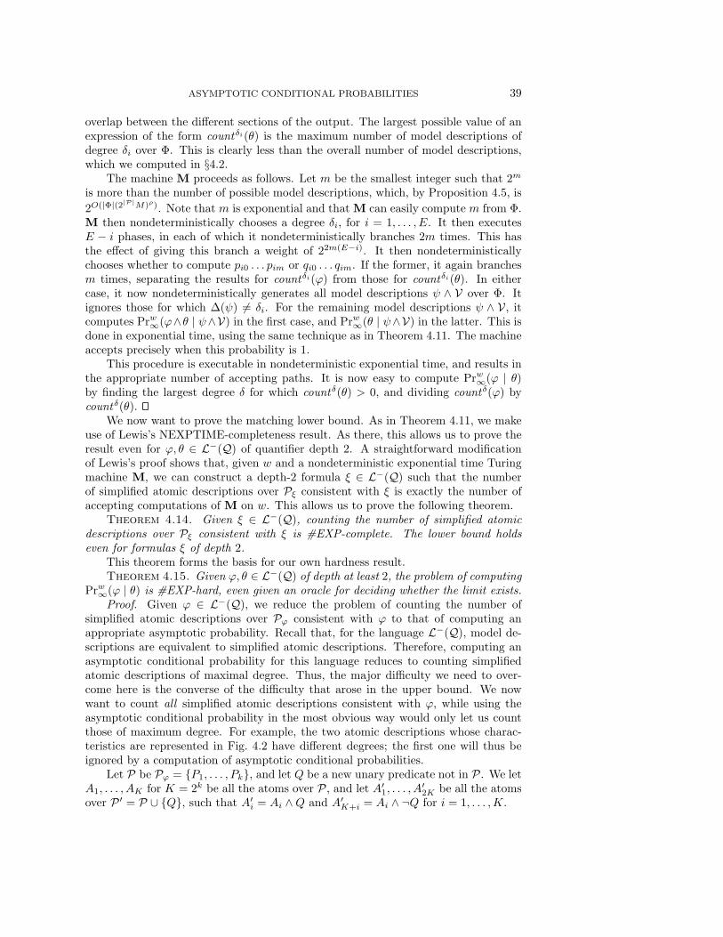
ASYMPTOTIC CONDITIONAL PROBABILITIES 39
overlap between the different sections of the output. The largest possible value of anexpression of the form countδi(θ) is the maximum number of model descriptions ofdegree δi over Φ. This is clearly less than the overall number of model descriptions,which we computed in §4.2.
The machine M proceeds as follows. Let m be the smallest integer such that 2m
is more than the number of possible model descriptions, which, by Proposition 4.5, is2O(|Φ|(2|P|M)ρ). Note that m is exponential and that M can easily compute m from Φ.M then nondeterministically chooses a degree δi, for i = 1, . . . , E. It then executesE − i phases, in each of which it nondeterministically branches 2m times. This hasthe effect of giving this branch a weight of 22m(E−i). It then nondeterministicallychooses whether to compute pi0 . . . pim or qi0 . . . qim. If the former, it again branchesm times, separating the results for countδi(ϕ) from those for countδi(θ). In eithercase, it now nondeterministically generates all model descriptions ψ ∧ V over Φ. Itignores those for which ∆(ψ) 6= δi. For the remaining model descriptions ψ ∧ V, itcomputes Prw∞(ϕ∧θ | ψ∧V) in the first case, and Prw∞(θ | ψ∧V) in the latter. This isdone in exponential time, using the same technique as in Theorem 4.11. The machineaccepts precisely when this probability is 1.
This procedure is executable in nondeterministic exponential time, and results inthe appropriate number of accepting paths. It is now easy to compute Prw∞(ϕ | θ)by finding the largest degree δ for which countδ(θ) > 0, and dividing countδ(ϕ) bycountδ(θ).
We now want to prove the matching lower bound. As in Theorem 4.11, we makeuse of Lewis’s NEXPTIME-completeness result. As there, this allows us to prove theresult even for ϕ, θ ∈ L−(Q) of quantifier depth 2. A straightforward modificationof Lewis’s proof shows that, given w and a nondeterministic exponential time Turingmachine M, we can construct a depth-2 formula ξ ∈ L−(Q) such that the numberof simplified atomic descriptions over Pξ consistent with ξ is exactly the number ofaccepting computations of M on w. This allows us to prove the following theorem.
Theorem 4.14. Given ξ ∈ L−(Q), counting the number of simplified atomicdescriptions over Pξ consistent with ξ is #EXP-complete. The lower bound holdseven for formulas ξ of depth 2.
This theorem forms the basis for our own hardness result.Theorem 4.15. Given ϕ, θ ∈ L−(Q) of depth at least 2, the problem of computing
Prw∞(ϕ | θ) is #EXP-hard, even given an oracle for deciding whether the limit exists.Proof. Given ϕ ∈ L−(Q), we reduce the problem of counting the number of
simplified atomic descriptions over Pϕ consistent with ϕ to that of computing anappropriate asymptotic probability. Recall that, for the language L−(Q), model de-scriptions are equivalent to simplified atomic descriptions. Therefore, computing anasymptotic conditional probability for this language reduces to counting simplifiedatomic descriptions of maximal degree. Thus, the major difficulty we need to over-come here is the converse of the difficulty that arose in the upper bound. We nowwant to count all simplified atomic descriptions consistent with ϕ, while using theasymptotic conditional probability in the most obvious way would only let us countthose of maximum degree. For example, the two atomic descriptions whose charac-teristics are represented in Fig. 4.2 have different degrees; the first one will thus beignored by a computation of asymptotic conditional probabilities.
Let P be Pϕ = P1, . . . , Pk, and let Q be a new unary predicate not in P. We letA1, . . . , AK for K = 2k be all the atoms over P, and let A′1, . . . , A
′2K be all the atoms
over P ′ = P ∪ Q, such that A′i = Ai ∧Q and A′K+i = Ai ∧ ¬Q for i = 1, . . . ,K.
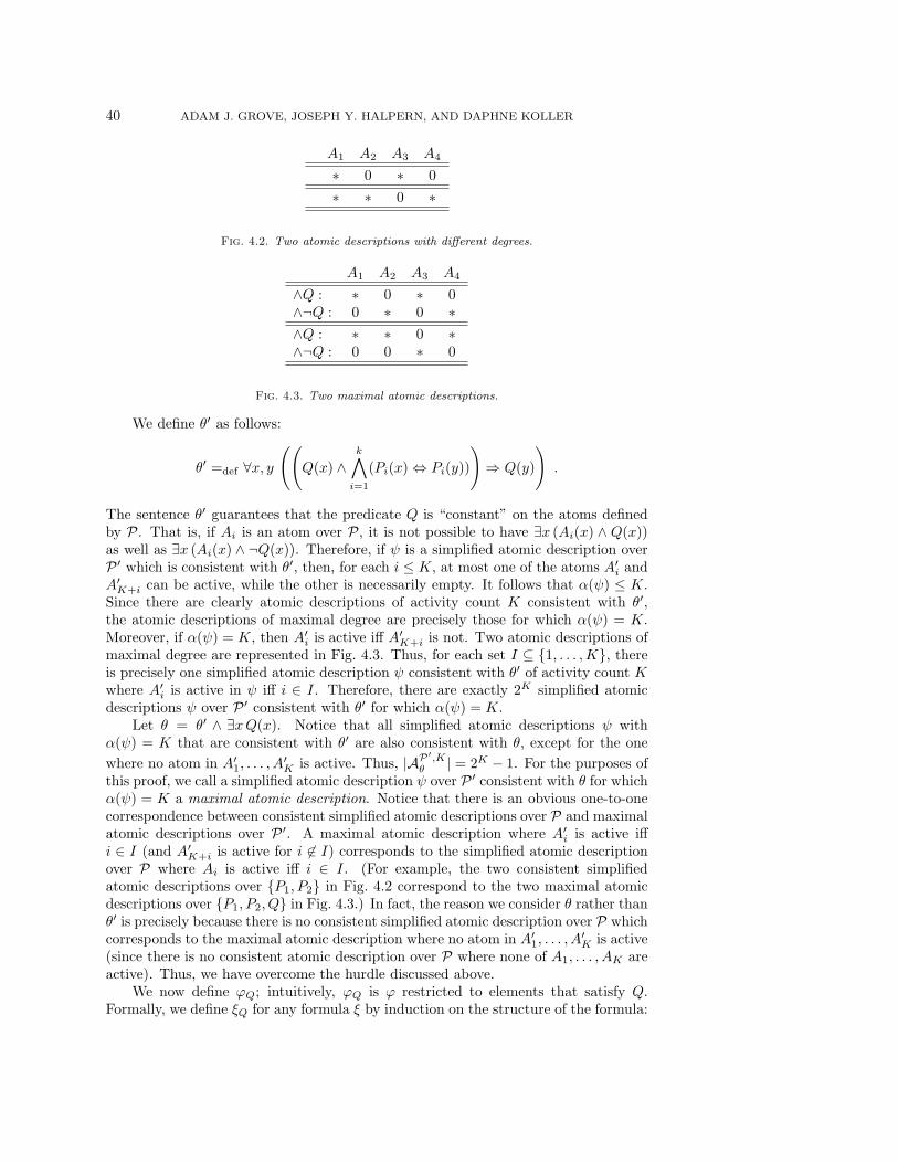
40 ADAM J. GROVE, JOSEPH Y. HALPERN, AND DAPHNE KOLLER
A1 A2 A3 A4
∗ 0 ∗ 0∗ ∗ 0 ∗
Fig. 4.2. Two atomic descriptions with different degrees.
A1 A2 A3 A4
∧Q : ∗ 0 ∗ 0∧¬Q : 0 ∗ 0 ∗∧Q : ∗ ∗ 0 ∗∧¬Q : 0 0 ∗ 0
Fig. 4.3. Two maximal atomic descriptions.
We define θ′ as follows:
θ′ =def ∀x, y
((Q(x) ∧
k∧i=1
(Pi(x)⇔ Pi(y))
)⇒ Q(y)
).
The sentence θ′ guarantees that the predicate Q is “constant” on the atoms definedby P. That is, if Ai is an atom over P, it is not possible to have ∃x (Ai(x) ∧ Q(x))as well as ∃x (Ai(x) ∧ ¬Q(x)). Therefore, if ψ is a simplified atomic description overP ′ which is consistent with θ′, then, for each i ≤ K, at most one of the atoms A′i andA′K+i can be active, while the other is necessarily empty. It follows that α(ψ) ≤ K.Since there are clearly atomic descriptions of activity count K consistent with θ′,the atomic descriptions of maximal degree are precisely those for which α(ψ) = K.Moreover, if α(ψ) = K, then A′i is active iff A′K+i is not. Two atomic descriptions ofmaximal degree are represented in Fig. 4.3. Thus, for each set I ⊆ 1, . . . ,K, thereis precisely one simplified atomic description ψ consistent with θ′ of activity count Kwhere A′i is active in ψ iff i ∈ I. Therefore, there are exactly 2K simplified atomicdescriptions ψ over P ′ consistent with θ′ for which α(ψ) = K.
Let θ = θ′ ∧ ∃xQ(x). Notice that all simplified atomic descriptions ψ withα(ψ) = K that are consistent with θ′ are also consistent with θ, except for the onewhere no atom in A′1, . . . , A
′K is active. Thus, |AP
′,Kθ | = 2K − 1. For the purposes of
this proof, we call a simplified atomic description ψ over P ′ consistent with θ for whichα(ψ) = K a maximal atomic description. Notice that there is an obvious one-to-onecorrespondence between consistent simplified atomic descriptions over P and maximalatomic descriptions over P ′. A maximal atomic description where A′i is active iffi ∈ I (and A′K+i is active for i 6∈ I) corresponds to the simplified atomic descriptionover P where Ai is active iff i ∈ I. (For example, the two consistent simplifiedatomic descriptions over P1, P2 in Fig. 4.2 correspond to the two maximal atomicdescriptions over P1, P2, Q in Fig. 4.3.) In fact, the reason we consider θ rather thanθ′ is precisely because there is no consistent simplified atomic description over P whichcorresponds to the maximal atomic description where no atom in A′1, . . . , A
′K is active
(since there is no consistent atomic description over P where none of A1, . . . , AK areactive). Thus, we have overcome the hurdle discussed above.
We now define ϕQ; intuitively, ϕQ is ϕ restricted to elements that satisfy Q.Formally, we define ξQ for any formula ξ by induction on the structure of the formula:

ASYMPTOTIC CONDITIONAL PROBABILITIES 41
• ξQ = ξ for any atomic formula ξ,• (¬ξ)Q = ¬ξQ,• (ξ ∧ ξ′)Q = ξQ ∧ ξ′Q,• (∀y ξ(y))Q = ∀y (Q(y)⇒ ξQ(y)).
Note that the size of ϕQ is linear in the size of ϕ. The one-to-one mapping discussedabove from simplified atomic descriptions to maximal atomic descriptions gives us aone-to-one mapping from simplified atomic descriptions over P consistent with ϕ tomaximal atomic descriptions consistent with ϕQ ∧ ∃xQ(x). This is true because amodel satisfies ϕQ iff the same model restricted to elements satisfying Q satisfies ϕ.Thus, the number of model descriptions over P consistent with ϕ is precisely |AP
′,KϕQ∧θ|.
From Corollary 3.36, it follows that
Prw∞(ϕQ | θ) =|AP
′,KϕQ∧θ|
|AP′,Kθ |=|APϕ |
2K − 1.
Thus, the number of simplified atomic descriptions over P consistent with ϕ is (2K −1)Prw∞(ϕQ | θ). This proves the lower bound.
As in Theorem 4.8, we can also show that any nontrivial approximation of theasymptotic probability is hard, even if we restrict to sentences of depth 2.
Theorem 4.16. Fix rational numbers 0 ≤ r1 ≤ r2 ≤ 1 such that [r1, r2] 6= [0, 1].For ϕ, θ ∈ L−(Q) of depth at least 2, the problem of deciding whether Prw∞(ϕ | θ) ∈[r1, r2] is both NEXPTIME-hard and co-NEXPTIME-hard, even given an oracle fordeciding whether the limit exists.
Proof. Let us begin with the case where r1 = 0 and r2 < 1. Consider anyϕ ∈ L−(Q) of depth at least 2, and assume without loss of generality that P =Pϕ = P1, . . . , Pk. Choose Q /∈ P, let P ′ = P ∪ Q, and let ξ be ∀x(P1(x) ∧ . . . ∧Pk(x) ∧Q(x)). We consider Prw∞(ϕ | ϕ ∨ ξ). Clearly ϕ ∨ ξ is satisfiable, so that thisasymptotic probability is well defined. If ϕ is unsatisfiable, then Prw∞(ϕ | ϕ ∨ ξ) = 0.On the other hand, if ϕ is satisfiable, then αP(ϕ) = j > 0 for some j. It is easyto see that αP
′(ϕ) = αP
′(ϕ ∨ ξ) = 2j. Moreover, ϕ and ϕ ∨ ξ are consistent with
precisely the same simplified atomic descriptions with 2j active atoms. This is truesince αP
′(ξ) = 1 < 2j. It follows that if ϕ is satisfiable, then Prw∞(ϕ | ϕ ∨ ξ) = 1.
Thus, we have that Prw∞(ϕ | ϕ ∨ ξ) is either 0 or 1, depending on whether ornot ϕ is satisfiable. Thus, Prw∞(¬ϕ | ϕ ∨ ξ) is in [r1, r2] iff ϕ is satisfiable; similarly,Prw∞(¬ϕ | ¬ϕ ∨ ξ) is in [r1, r2] iff ϕ is valid. By Theorem 4.10, it follows that thisapproximation problem is both NEXPTIME-hard and co-NEXPTIME-hard.
If r1 = q/p > 0, we construct sentences ϕr1 and θr1 of depth 2 in L−(Q) suchthat Prw∞(ϕr1 | θr1) = r1.11 Choose ` = dlog pe, and let P ′′ = Q1, . . . , Q` be a setof predicates such that P ′′∩P ′ = ∅. Let A1, . . . , A2` be the set of atoms over P ′′. Wedefine θr1 to be
∃1x (A1(x) ∨A2(x) ∨ . . . ∨Ap(x)).
Similarly, ϕr1 is defined as
∃1x (A1(x) ∨A2(x) ∨ . . . ∨Aq(x)).
11The sentences constructed in Theorem 4.8 for the same purpose will not serve our purpose inthis theorem, since they used unbounded quantifier depth.

42 ADAM J. GROVE, JOSEPH Y. HALPERN, AND DAPHNE KOLLER
Recall from §3.1 that the construct “∃1x” can be defined in terms of a formula ofquantifier depth 2. There are exactly p atomic descriptions of size 2 of maximaldegree consistent with θr1 ; each has one element in one of the atoms A1, . . . , Ap andno elements in the rest of the atoms among A1, . . . , Ap, with all the remaining atoms(those among Ap+1, . . . , A2`) being active. Among these atomic descriptions, q arealso consistent with ϕr1 . Therefore, Prw∞(ϕr1 | θr1) = q/p. Since the predicatesoccurring in ϕr1 , θr1 are disjoint from P ′, it follows that
Prw∞(ϕ ∧ ϕr1 | (ϕ ∨ ξ) ∧ θr1) = Prw∞(ϕ | ϕ ∨ ξ) · Prw∞(ϕr1 | θr1) = Prw∞(ϕ | ϕ ∨ ξ) · r1.
This is equal to r1 (and hence is in [r1, r2]) if and only if ϕ is satisfiable, and is 0other- wise.
The lower bounds in this section all hold provided we consider formulas whosequantification depth is at least 2. Can we do better if we restrict to formulas of quan-tification depth at most 1? As is suggested by Table 1.1, we can. The complexitiestypically drop by an exponential factor. For example, checking well-definedness be-comes NP-complete rather than NEXPTIME-complete. For the problem of computingprobabilities for formulas with quantification depth 1, we know that the problem is inPSPACE, and is (at least) #P-hard. Finally, the problem of approximating probabil-ities is hard for both NP and co-NP. A detailed analysis of these results can be foundin [27]; some related work for a propositional language has been done by Roth [35].
4.5. Infinite vocabulary—the general case. In §4.4 we investigated the com-plexity of asymptotic conditional probabilities when the (infinite) vocabulary satisfiescertain restrictions. As we now show, the results there were tight in the sense that therestrictions cannot be weakened. We examine the complexity of the general case, inwhich the vocabulary is infinite with no bound on predicates’ arities and/or in whichequality can be used.
The problem of checking if Prw∞(ϕ | θ) is well defined is still NEXPTIME-complete. Theorem 4.11 (which had no restrictions) still applies. However, the com-plexity of the other problems we consider does increase. It can be best describedin terms of the complexity class TA(EXP,LIN)—the class of problems that can besolved by an exponential time ATM with a linear number of alternations. The classTA(EXP,LIN) also arises in the study of unconditional probabilities where there is nobound on the arity of the predicates. Grandjean [20] proved a TA(EXP,LIN) upperbound for computing whether the unconditional probability is 0 or 1 in this case, andImmerman [4] proved a matching lower bound. Of course, Grandjean’s result can beviewed as a corollary of Theorem 4.3. Immerman’s result, which has not, to the bestof our knowledge, appeared in print, is a corollary of Theorem 4.18 which we provein this section.
To capture the complexity of computing the asymptotic probability in the generalcase, we use a counting class #TA(EXP,LIN) that corresponds to TA(EXP,LIN).To define this class, we restrict attention to the class of ATMs whose initial statesare existential. Given such an ATM M, we define an initial existential path in thecomputation tree of M on input w to be a path in this tree, starting at the initialstate, such that every node on the path corresponds to an existential state exceptfor the last node, which corresponds to a universal or an accepting state. That is,an initial existential path is a maximal path that starts at the root of the tree andcontains only existential nodes except for the last node in the path. We say that aninteger-valued function f : 0, 1∗ → IN is in #TA(EXP,LIN) if there is a machineM in the class TA(EXP,LIN) such that, for all w, f(w) is the number of existential

ASYMPTOTIC CONDITIONAL PROBABILITIES 43
paths in the computation tree of M on input w whose last node is accepting (recallthat we defined a notion of “accepting” for any node in the tree in §4.1). We extendthe definition of #TA(EXP,LIN) to apply to non-integer-valued functions and define#TA(EXP,LIN )-easy just as we did before with #P and #EXP in §4.4.
We start with the upper bound.Theorem 4.17. For ϕ ∈ L(Ω) and θ ∈ L(Υ), the function Prw∞(ϕ | θ) is in
#TA(EXP,LIN ).Proof. Let Φ = Ωϕ∧θ, let Ψ = Υϕ∧θ, and let ρ be the maximum arity of a
predicate in Φ. The proof proceeds precisely as in Theorem 4.13. We compute, for eachdegree δ, the values countδ(θ) and countδ(ϕ). This is done by nondeterministicallygenerating model descriptions ψ ∧ V over Φ, branching according to the degree of ψ,and computing Prw∞(ϕ ∧ θ | ψ ∧ V) and Prw∞(θ | ψ ∧ V) using a TA(EXP,LIN) Turingmachine.
To see that this is possible, recall from Proposition 4.5 that the length of a modeldescription over Φ is O(|Φ|(2|P|M)ρ). This is exponential in |Φ| and ρ, both of whichare at most |ϕ ∧ θ|. Therefore, it is possible to guess a model description in expo-nential time. Similarly, as we saw in the proof of Theorem 4.13, only exponentiallymany nondeterministic guesses are required to separate the output so that countscorresponding to different degrees do not overlap. These guesses form the initial non-deterministic stage of our TA(EXP,LIN) Turing machine. Note that it is necessary toconstruct the rest of the Turing machine so that a universal state always follows thisinitial stage, so that each guess corresponds exactly to one initial existential path;however, this is easy to arrange.
For each model description ψ ∧ V so generated, we compute Prw∞(θ | ψ ∧ V)or Prw∞(ϕ ∧ θ | ψ ∧ V) as appropriate, accepting if the conditional probability is1. It follows immediately from Theorem 4.3 and the fact that there can only beexponentially many named elements in any model description we generate that thiscomputation is in TA(EXP,LIN). Thus, the problem of computing Prw∞(ϕ | θ) is in#TA(EXP,LIN).
We now want to prove the matching lower bound. Moreover, we would like toshow that the restrictions from §4.4 cannot be weakened. Recall from Theorem 4.13that the #EXP upper bound held under one of two conditions: either (a) ϕ and θare both unary, or (b) the vocabulary is arity-bounded and θ does not use equality.To show that (a) is tight, we show that the #TA(EXP,LIN) lower bound holds evenif we allow ϕ and θ to use only binary predicates and equality. (The use of equalityis necessary, since without it we know from (b) that the problem is #EXP-easy.) Toshow that (b) is tight, we show that the lower bound holds for a non-arity-boundedvocabulary, but without allowing equality in θ. Neither lower bound requires the useof constants.
The proof of the lower bounds is lengthy, but can be simplified somewhat by someassumptions about the construction of the TA(EXP,LIN) machines we consider. Themain idea is that the existential “guesses” being made in the initial phase should beclearly distinguished from the rest of the computation. To achieve this, we assumethat the Turing machine has an additional guess tape, and the initial phase of everycomputation consists of nondeterministically generating a guess string γ which iswritten on the new tape. The machine then proceeds with a standard alternatingcomputation, but with the possibility of reading the bits on the guess tape.
More precisely, from now on we make the following assumptions about an ATMM. Consider any increasing functions T (n) and A(n) (in essence, these correspond

44 ADAM J. GROVE, JOSEPH Y. HALPERN, AND DAPHNE KOLLER
to the time complexity and number of alternations), and let w be an input of size n.We assume:
• M has two tapes and two heads (one for each tape). Both tapes are one-wayinfinite to the right.• The first tape is a work tape, which initially contains only the string w.• M has an initial nondeterministic phase, during which its only action is to
nondeterministically generate a string γ of zeros and ones, and write thisstring on the second tape (the guess tape). The string γ is always of lengthT (n). Moreover, at the end of this phase, the work tape is as in the initialconfiguration, the guess tape contains only γ, the heads are at the beginningof their respective tapes, and the machine is in a distinguished universal states0.• After the initial phase, the guess tape is never changed.• After the initial phase, M takes at most T (n) steps on each branch of its
computation tree, and makes exactly A(n)− 1 alternations before entering aterminal (accepting or rejecting) state.• The state before entering a terminal state is always an existential state
(i.e., A(n) is odd).Let M′ be any (unrestricted) TA(T ,A) machine that “computes” an integer func-
tion f . It is easy to construct some M satisfying the restrictions above that alsocomputes f . The machine M first generates the guess string γ, and then simulatesM′. At each nondeterministic branching point in the initial existential phase of M′,M uses the next bit of the string γ to dictate which choice to take. Observe that thisphase is deterministic (given γ), and can thus be folded into the following universalphase. (Deterministic steps can be viewed as universal steps with a single successor.)If not all the bits in γ are used, M continues the execution of M′, but checks in par-allel that the unused bits of γ are all 0’s. If not, M rejects. It is easy to see that onany input w, M has the same number of accepting paths as M′, and therefore acceptsthe same function f . Moreover, M has the same number of alternations as M′, andat most a constant factor blowup in the running time.12 This shows that it will besufficient to prove our hardness results for the class #TA(EXP,LIN) by consideringonly those machines that satisfy these restrictions. For the remainder of this sectionwe will therefore assume that all ATMs are of this type.
Let M be such an ATM and let w be an input of size n. We would like toencode the computation of M on w using a pair of formulas ϕw, θw. (Of course, theseformulas depend on M as well, but we suppress this dependence.) Our first theoremshows how to encode part of this computation: given some appropriate string γ oflength T (n), we construct formulas that encode the computation of M immediatelyfollowing the initial phase of guessing γ. More precisely, we say that M accepts wgiven γ if, on input w, the initial existential path during which M writes γ on theguess tape leads to an accepting node. We construct formulas ϕw,γ and θw,γ suchthat Prw∞(ϕw,γ | θw,γ) is either 0 or 1, and is equal to 1 iff M accepts w given γ.
We do not immediately want to specify the process of guessing γ, so our initialconstruction will not commit to this. For a predicate R, let ϕ[R] be a formula thatuses the predicate R. Let ξ be another formula that has the same number of freevariables as the arity of R. Then ϕ[ξ] is the formula where every occurrence of R isreplaced with the formula ξ, with an appropriate substitution of the arguments of R
12For ease of presentation, we can and will (somewhat inaccurately, but harmlessly) ignore thisconstant factor and say that the time complexity of M is, in fact, T (n).
ASYMPTOTIC CONDITIONAL PROBABILITIES 45
for the free variables in ξ.Theorem 4.18. Let M be a TA(T ,A) machine as above, where T (n) = 2t(n) for
some polynomial t(n) and A(n) = O(n). Let w be an input string of length n, andγ ∈ 0, 1T (n) be a guess string.
(a) For a unary predicate R, there exist formulas ϕw[R], ξγ ∈ L(Ω) and θw ∈L(Υ) such that Prw∞(ϕw[ξγ ] | θw) = 1 iff M accepts w given γ and is 0otherwise. Moreover, ϕw uses only predicates with arity 2 or less.
(b) For a binary predicate R, there exist formulas ϕ′w[R], ξ′γ ∈ L(Ω) such thatPrw∞(ϕ′w[ξ′γ ] | true) = 1 iff M accepts w given γ and is 0 otherwise.
The formulas ϕw[R], θw, and ϕ′w[R] are independent of γ, and their length is polyno-mial in the representation of M and w. Moreover, none of the formulas constructeduse any constant symbols.
Proof. Let Γ be the tape alphabet of M and let S be the set of states of M. Wewill identify an instantaneous description (ID) of length ` of M with a string Σ` forΣ = ΣW ×ΣG, where ΣW is Γ∪ (Γ×S) and ΣG is (0, 1∪ (0, 1×h)). We thinkof the ΣW component of the ith element in a string as describing the contents of theith location in the work tape and also, if the tape head is at location i, the state ofthe Turing machine. The ΣG component describes the contents of the ith locationin the guess tape (whose alphabet is 0, 1) and whether the guess tape’s head ispositioned there. Of course, we consider only strings in which exactly one elementin Γ × S appears in the first component and exactly one element in 0, 1 × happears in the second component. Since M halts within T (n) steps (not counting theguessing process, which we treat separately), we need only deal with IDs of length atmost T (n). Without loss of generality, assume all IDs have length exactly T (n). (Ifnecessary, we can pad shorter IDs with blanks.)
In both parts of the theorem, IDs are encoded using the properties of domainelements. In both cases, the vocabulary contains predicates whose truth value withrespect to certain combinations of domain elements represent IDs. The only differencebetween parts (a) and (b) is in the precise encoding used. We begin by showing theencoding for part (a).
In part (a), we use the sentence θw to define T (n) named elements. This is possiblesince θw is allowed to use equality. Each ID of the machine will be represented usinga single domain element. The properties of the ID will be encoded using the relationsbetween the domain element representing it and the named elements. More precisely,assume that the vocabulary has t(n) unary predicates P1, . . . , Pt(n), and one additionalunary predicate P ∗. The domain is divided into two parts: the elements satisfyingP ∗ are the named elements used in the process of encoding IDs, while the elementssatisfying ¬P ∗ are used to actually represent IDs. The formula θw asserts (usingequality) that each of the atoms A over P ∗, P1, . . . , Pt(n) in which P ∗ (as opposedto ¬P ∗) is one of the conjuncts contains precisely one element:
∀x, y
P ∗(x) ∧ P ∗(y) ∧t(n)∧i=1
(Pi(x)⇔ Pi(y))
⇒ x = y
.
Note that θw has polynomial length and is independent of γ.We can view an atom A over P ∗, P1, . . . , Pt(n) in which P ∗ is one of the con-
juncts as encoding a number between 0 and T (n)−1, written in binary: if A containsPj rather than ¬Pj , then the jth bit of the encoded number is 1; otherwise it is 0.(Recall that T (n), the running time of M, is 2t(n).) In the following, we let Ai, for

46 ADAM J. GROVE, JOSEPH Y. HALPERN, AND DAPHNE KOLLER
i = 0, . . . , T (n)− 1, denote the atom corresponding to the number i according to thisscheme. Let ei be the unique element in the atom Ai for i = 0, . . . , T (n)− 1. Whenrepresenting an ID using a domain element d (where ¬P ∗(d)), the relation betweend and ei is used to represent the ith coordinate in the ID represented by d. Assumethat the vocabulary has a binary predicate Rσ for each σ ∈ Σ. Roughly speaking, wesay that the domain element d represents the ID σ0 . . . σT (n)−1 if Rσi(d, ei) holds fori = 0, . . . , T (n)− 1. More precisely, we say that d represents σ0 . . . σT (n)−1 if
¬P ∗(d) ∧T (n)−1∧i=0
∀y
Ai(y)⇒
Rσi(d, y) ∧∧
σ′∈Σ−σi
¬Rσ′(d, y)
.
Note that not every domain element d such that ¬P ∗(d) holds encodes a valid ID.However, the question of which ID, if any, is encoded by a domain element d dependsonly on the relations between d and the finite set of elements e0, . . . , eT (n)−1. Thisimplies that, with asymptotic probability 1, every ID will be encoded by some domainelement. More precisely, let ID(x) = σ0 . . . σT (n)−1 be a formula which is true if xdenotes an element that represents σ0 . . . σT (n)−1. (It should be clear that such aformula is indeed expressible in our language.) Then for each ID σ0 . . . σT (n)−1 wehave
Prw∞(∃x (ID(x) = σ0 . . . σT (n)−1) | θw) = 1.
For part (b) of the theorem, we must represent IDs in a different way becausewe are not allowed to condition on formulas that use equality. Therefore, we cannotcreate an exponential number of named elements using a polynomial-sized formula.The encoding we use in this case uses two domain elements per ID rather than one.We now assume that the vocabulary Ω contains a t(n)-ary predicate Rσ for eachsymbol σ ∈ Σ. Note that this uses the assumption that there is no bound on the arityof predicates in Ω. For i = 0, . . . , T (n)− 1, let bit(n) . . . b
i1 be the binary encoding of i.
We say that the pair (d0, d1) of domain elements represents the ID σ0 . . . σT (n)−1 if
d0 6= d1 ∧T (n)−1∧i=0
Rσi(dbi1 , . . . , dbit(n)) ∧
∧σ′∈Σ−σi
¬Rσ′(dbi1 , . . . , dbit(n))
.
Again, we can define a formula in our language ID(x0, x1) = σ0 . . . σT (n)−1 whichis true if x0, x1 denote a pair of elements that represent σ0 . . . σT (n)−1. As before,observe that for each ID σ0 . . . σT (n)−1 we have
Prw∞(∃x0, x1 (ID(x0, x1) = σ0 . . . σT (n)−1) | true) = 1.
In both case (a) and case (b), we can construct formulas polynomial in the sizeof M and w that assert certain properties. For example, in case (a), Rep(x) is true ofa domain element d if and only if d encodes an ID. In this case, Rep(x) is the formula
¬P ∗(x) ∧ ∀y(P ∗(y)⇒
∨σ∈ΣRσ(x, y)
)∧
∃!y (P ∗(y) ∧∨σ∈((Γ×S)×ΣG)Rσ(x, y)) ∧ ∃!y (P ∗(y) ∧
∨σ∈(ΣW×(0,1×h))Rσ(x, y))
where∨
is an abbreviation whose meaning is that precisely one of its disjuncts istrue.

ASYMPTOTIC CONDITIONAL PROBABILITIES 47
In case (b), Rep(x0, x1) is true of a pair (d0, d1) if and only if it encodes an ID.The construction is similar. For instance, the conjunct of Rep(x0, x1) asserting thateach tape position has a uniquely defined content is
x0 6= x1 ∧ ∀z1, . . . , zt(n)
t(n)∧i=1
(zi = x0 ∨ zi = x1)
⇒ ∨σ∈Σ
Rσ(z1, . . . , zt(n))
.
Except for this assertion, the construction for the two cases is completely parallelgiven the encoding of IDs. We will therefore restrict the remainder of the discussionto case (a). Other relevant properties of an ID that we can formulate are:
• Acc(x) (resp., Univ(x), Exis(x)) is true of a domain element d if and only if dencodes an ID and the state in ID(d) is an accepting state (resp., a universalstate, an existential state).• Step(x, x′) is true of elements d and d′ if and only if both d and d′ encode
IDs and ID(d′) can follow from ID(d) in one step of M.• Comp(x, x′) is true of elements d and d′ if and only if both d and d′ encode
IDs, and ID(d′) is the final ID in a maximal nonalternating path starting atID(d) in the computation tree of M, and the length of this path is at mostT (n). A maximal nonalternating path is either a path all of whose statesare existential except for the last one (which must be universal or accepting),or a path all of whose states are universal except for the last one. We canconstruct Comp using a divide and conquer argument, so that its length ispolynomial in t(n).
We remark that Acc, Step, etc. are not new predicate symbols in the language. Rather,they are complex formulas described in terms of the basic predicates Rσ. We omitdetails of their construction here; these can be found in [20].
It remains only to describe the formula that encodes the initial configuration ofM on input w. Since we are interested in the behavior of M given a particular guessstring γ, we begin by encoding the computation of M after the initial nondeterministicphase; that is, after the string γ is already written on the guess tape and the rest ofthe machine is back in its original state. We now construct the formula Init [R](x)that describes the initial configuration. This formula takes R as a parameter, and hasthe form Init ′(x)∧R(x). The formulas substituted for R(x) will correspond (in a waydiscussed below) to possible guesses γ.
We begin by considering case (a). We assume the existence of an additional binarypredicate B0. It is easy to write a polynomial-length formula Init ′(x) which is trueof a domain element d if and only if d represents an ID where: (a) the state is thedistinguished state s0 entered after the nondeterministic guessing phase, (b) the worktape contains only w, (c) the heads are at the beginning of their respective tapes,and (d) for all i, the ith location of the guess tape contains 0 iff B0(d, ei). Here eiis, as before, the unique element in atom Ai. Note that the last constraint can berepresented polynomially using the formula
∀y
P ∗(y)⇒
B0(x, y)⇔∨
σ∈ΣW×0,(0,h)
Rσ(x, y)
.
We also want to find a formula ξγ that can constrain B0 to reflect the guess γ.This formula, which serves as a possible instantiation for R, does not have to be ofpolynomial size. We define it as follows, where for convenience, we use B1 as an

48 ADAM J. GROVE, JOSEPH Y. HALPERN, AND DAPHNE KOLLER
abbreviation for ¬B0:
ξγ(x) =def
T (n)−1∧i=0
∀y (Ai(y)⇒ Bγi(x, y)) .(4.1)
Note that this is of exponential length.In case (b), the relation of the guess string γ to the initial configuration is essen-
tially the same modulo the modifications necessary due to the different representationof IDs. We only sketch the construction. As in case (a), we add a predicate B′0, butin this case of arity t(n). Again, the predicate B′0 represents the locations of the 0’s inthe guess tape following the initial nondeterministic phase. The specification of thedenotation of this predicate is done using an exponential-sized formula ξ′γ , as follows(again taking B′1 to be an abbreviation for ¬B′0):
ξ′γ(x0, x1) =def B′γ0(x0, . . . , x0, x0)∧B′γ1(x0, . . . , x0, x1)∧. . .∧B′γT (n)−1
(x1, . . . , x1, x1).
Using these formulas, we can now write a formula expressing the assertion that Maccepts w given γ. In writing these formulas, we make use of the assumptions madeabout M (that it is initially in the state immediately following the initial guessingphase, that all computation paths make exactly A(n) alternations, and so on). Theformula ϕw[R] has the following form:
∃x1 (Init [R](x1) ∧ ∀x2 (Comp(x1, x2)⇒ ∃x3 (Comp(x2, x3) ∧ ∀x4 (Comp(x3, x4)⇒ . . .∃xA(n) (Comp(xA(n)−1, xA(n)) ∧Acc(xA(n))) . . .)))).
It is clear from the construction that ϕw[R] does not depend on γ and that its lengthis polynomial in the representations of M and w.
Now supposeW is a world satisfying θw in which every possible ID is representedby at least one domain element. (As we remarked above, a random world has thisproperty with asymptotic probability 1.) Then it is straightforward to verify thatϕw[ξγ ] is true in W iff M accepts w. Therefore Prw∞(ϕw[ξγ ] | θw) = 1 iff M acceptsw given γ and 0 otherwise. Similarly, in case (b), we have shown the construction ofanalogous formulas ϕ′w[R], for a binary predicate R, and ξ′γ such that Prw∞(ϕ′w[ξ′γ ] |true) = 1 iff M accepts w given γ, and is 0 otherwise.
We can now use the above theorem in order to prove the #TA(EXP,LIN) lowerbound.
Theorem 4.19. For ϕ ∈ L(Ω) and θ ∈ L(Υ), computing Prw∞(ϕ | θ) is#TA(EXP,LIN )-hard. The lower bound holds even if ϕ, θ do not mention constantsymbols and either (a) ϕ uses no predicate of arity > 2, or (b) θ uses no equality.
Proof. Let M be a TA(EXP,LIN) Turing machine of the restricted type discussedearlier, and let w be an input of size n. We would like to construct formulas ϕ, θ suchthat from Prw∞(ϕ | θ) we can derive the number of accepting computations of M on w.The number of accepting initial existential paths of such a Turing machine is preciselythe number of guess strings γ such that M accepts w given γ. In Theorem 4.18, weshowed how to encode the computation of such a machine M on input w given anondeterministic guess γ. We now show how to force an asymptotic conditionalprobability to count guess strings appropriately.
As in Theorem 4.18, let T (n) = 2t(n), and let P ′ = P ′1, . . . , P ′t(n) be new unarypredicates not used in the construction of Theorem 4.18. As before, we can view anatom A′ over P ′ as representing a number in the range 0, . . . , T (n)− 1: if A containsP ′j , then the jth bit of the encoded number is 1; otherwise it is 0. Again, let A′i, for

ASYMPTOTIC CONDITIONAL PROBABILITIES 49
i = 0, . . . , T (n)− 1, denote the atom corresponding to the number i according to thisscheme. We can view a simplified atomic description ψ over P ′ as representing thestring γ = γ0 . . . γT (n)−1 such that γi is 1 if ψ contains the conjunct ∃z A′i(z), and0 if ψ contains its negation. Under this representation, for every string γ of lengthT (n), there is a unique simplified atomic description over P ′ that represents it; wedenote this atomic description ψγ . Note that ψγ is not necessarily a consistent atomicdescription, since the atomic description where all atoms are empty also denotes alegal string—that string where all bits are 0.
While it is possible to reduce the problem of counting accepting guess stringsto that of counting simplified atomic descriptions, this is not enough. After all, wehave already seen that computing asymptotic conditional probabilities ignores allatomic descriptions that are not of maximal degree. We deal with this problem as inTheorem 4.15. Let Q be a new unary predicate, and let θ′ be, as in Theorem 4.15,the sentence
∀x, y
Q(x) ∧t(n)∧j=1
(P ′j(x)⇔ P ′j(y))
⇒ Q(y)
.
Observe that here we use θ′ rather than the formula θ of Theorem 4.15, since we alsowant to count the “inconsistent” atomic description where all atoms are empty. Recallthat, assuming θ′, each simplified atomic description ψγ over P ′ corresponds preciselyto a single maximal atomic description ψ′γ over P ′ ∪ Q. We reduce the problemof counting accepting guess strings to that of counting maximal atomic descriptionsover P ′ ∪ Q.
We now consider cases (a) and (b) separately, beginning with the former. Fixa guess string γ. In Theorem 4.18, we constructed formulas ϕw[R], ξγ ∈ L(Ω) andθw ∈ L(Υ) such that Prw∞(ϕw[ξγ ] | θw) = 1 iff M accepts w given γ, and is 0 otherwise.Recall that the formula ξγ(x) (see equation (4.1)) sets the ith guess bit to be γi byforcing the appropriate one of B0(x, ei) and B1(x, ei) to hold, where ei is the uniqueelement in the atom Ai. In Theorem 4.18, this was done directly by reference to thebits γi. Now, we want to derive the correct bit values from ψγ , which tells us that theith bit is 1 iff ∃z A′i(z). The following formula ξ has precisely the desired property:
ξ(x) =def ∀y
P ∗(y)⇒
B1(x, y)⇔ ∃z
Q(z) ∧t(n)∧j=1
(Pj(y)⇔ P ′j(z))
.
Clearly, ψ′γ |= ξ ⇔ ξγ .Similarly, for case (b), the formula ξ′ is:
ξ′(x0, x1) =def ∀y1, . . . , yt(n)
t(n)∧j=1
(yj = x0 ∨ yj = x1)
⇒B′1(y1, . . . , yt(n))⇔ ∃z
Q(z) ∧t(n)∧j=1
(yj = x1 ⇔ P ′j(z))
.
As in part (a), ψ′γ |= ξ′ ⇔ ξ′γ .Now, for case (a), we want to compute the asymptotic conditional probability
Prw∞(ϕ[ξ] | θw ∧ θ′). In doing this computation, we will use the observation (whosestraightforward proof we leave to the reader) that if the symbols that appear in θ2 are

50 ADAM J. GROVE, JOSEPH Y. HALPERN, AND DAPHNE KOLLER
disjoint from those that appear in ϕ1 and θ1, then Prw∞(ϕ1 | θ1 ∧ θ2) = Prw∞(ϕ1 | θ1).Using this observation and the fact that all maximal atomic descriptions over P ′∪Qare equally likely given θw ∧ θ′, by straightforward probabilistic reasoning we obtain:
Prw∞(ϕw[ξ] | θw ∧ θ′) =∑ψ′γ
Prw∞(ϕw[ξ] | θw ∧ θ′ ∧ ψ′γ) · Prw∞(ψ′γ | θw ∧ θ′)
=1
2T (n)
∑ψ′γ
Prw∞(ϕw[ξ] | θw ∧ θ′ ∧ ψ′γ).
We observed before that ξ is equivalent to ξγ in worlds satisfying ψ′γ , and therefore
Prw∞(ϕw[ξ] | θw ∧ θ′ ∧ ψ′γ) = Prw∞(ϕw[ξγ ] | θw ∧ θ′ ∧ ψ′γ) = Prw∞(ϕw[ξγ ] | θw),
where the second equality follows from the observation that none of the vocabularysymbols in ψ′γ or θ′ appear anywhere in ϕw[ξγ ] or in θw. In Theorem 4.18, we provedthat Prw∞(ϕw[ξγ ] | θw) is equal to 1 if the ATM accepts w given γ and 0 if not. Wetherefore obtain that
Prw∞(ϕw[ξ] | θw ∧ θ′) =f(w)2T (n)
.
Since both ϕw[ξ] and θw ∧ θ′ are polynomial in the size of the representation of Mand in n = |w|, this concludes the proof for part (a). The completion of the proof forpart (b) is essentially identical.
It remains only to investigate the problem of approximating Prw∞(ϕ | θ) for thislanguage.
Theorem 4.20. Fix rational numbers 0 ≤ r1 ≤ r2 ≤ 1 such that [r1, r2] 6=[0, 1]. For ϕ, θ ∈ L(Ω), the problem of deciding whether Prw∞(ϕ | θ) ∈ [r1, r2] isTA(EXP,LIN )-hard, even given an oracle for deciding whether the limit exists.
Proof. For the case of r1 = 0 and r2 < 1, the result is an easy corollary ofTheorem 4.18. We can generalize this to the case of r1 > 0, using precisely the sametechnique as in Theorem 4.16.
4.6. Complexity for random structures. So far in this section, we haveinvestigated the complexity of various problems relating to the asymptotic conditionalprobability using the random-worlds method. We now deal with the same issues forthe case of random structures. It turns out that most of our results for random worldscarry through to random structures for trivial reasons.
First, consider the issue of well-definedness. By Proposition 2.3, well-definednessis equivalent for random worlds and random structures. Therefore, all of the resultsobtained for random worlds carry through unchanged for random structures.
For computing or approximating the limit, Theorem 3.37 allows us to restrictattention to unary vocabularies and unary sentences ϕ and θ. In particular, there isno need to duplicate the results in §4.5. For the remainder of this section, we analyzethe complexity of computing Prs,Ψ∞ (ϕ | θ) for ϕ, θ ∈ L(Ψ). As before, we can assumethat AΨ
ϕ∧θ ⊆ AΨθ .
The computational approach is essentially the same as that for random worlds.However, as we showed in §3.5, rather than partitioning θ into model descriptions, wecan make use of the assumption that the vocabulary is unary and instead partition itinto atomic descriptions ψ. That is, for a = αΨ(θ),
Prs,Ψ∞ (ϕ | θ) =1
|AΨ,aθ |·∑
ψ∈AΨ,a
Prw∞(ϕ | ψ)
(=|AΨ,a
ϕ∧θ||AΨ,a
θ |
).

ASYMPTOTIC CONDITIONAL PROBABILITIES 51
As for random worlds, we begin with the problem of computing 0-1 probabilities.In §4.1, we showed how to extend Grandjean’s algorithm to compute Prw∞(ϕ | ψ ∧V).Fix a unary vocabulary Ψ, and suppose that ψ ∧ V is a model description over Ψ,with n = ν(ψ). Recall from Proposition 3.21 that Prw∞(ϕ | ψ ∧ V) = Prw∞(ϕ |ψ∧∃x1, . . . , xnDV). However, in the unary case it is easy to see that ψ∧∃x1, . . . , xnDVis equivalent to ψ. This is because the only nontrivial properties of the named elementsgiven by V is which atom each of them satisfies and the equality relations betweenthe constants, and this information is already present in the atomic description ψ.
Therefore, we conclude that Prw∞(ϕ | ψ) is either 0 or 1, because this is so forPrw∞(ϕ | ψ ∧ V). Now recall that if ψ ∈ AΨ
ϕ then ψ implies ϕ. In this case, clearlyPrw∞(ϕ | ψ) = Prs,Ψ∞ (ϕ | ψ) = 1. Similarly, if ψ 6∈ AΨ
ϕ , then ψ is inconsistent withϕ and Prw∞(ϕ | ψ) = Prs,Ψ∞ (ϕ | ψ) = 0. So it follows that we can continue to useGrandjean’s algorithm, as described in §4.1, to compute Prs,Ψ∞ (ϕ | ψ).
Theorem 4.21. There exists an alternating Turing machine that takes as input afinite unary vocabulary Ψ, an atomic description ψ over Ψ, and a formula ϕ ∈ L(Ψ),and decides whether Prs,Ψ∞ (ϕ | ψ) is 0 or 1. The machine uses time O(|Ψ|2|P|(ν(ψ) +|ϕ|)) and has at most O((2|Ψ| + ν(ψ))|ϕ|) branches and O(|ϕ|) alternations.
As before, we can simulate the ATM deterministically.Corollary 4.22. There exists a deterministic Turing machine that takes as
input a finite unary vocabulary Ψ, an atomic description ψ over Ψ, and a formulaϕ ∈ L(Ψ), and decides whether Prw,Ψ∞ (ϕ | ψ) is 0 or 1. The machine uses time2O(|ϕ||Ψ| log(ν(ψ)+1)) and space O(|ϕ||Ψ| log(ν(ψ) + 1)).
We now analyze the complexity of computing Prs,Ψ∞ (ϕ | θ). We begin with thecase of a fixed finite vocabulary Ψ.
Theorem 4.23. Fix a finite unary vocabulary Ψ with at least one predicatesymbol. For ϕ, θ ∈ L(Ψ), the problem of computing Prs,Ψ∞ (ϕ | θ) is PSPACE-complete.Moreover, deciding if Prw∞(ϕ | true) = 1 is PSPACE-hard, even if ϕ ∈ L−(P).
Proof. By Corollaries 3.41 and 3.42, if ϕ, θ ∈ L−(P) and P ∈ Ψ, then Prw∞(ϕ |θ) = Prs,P∞ (ϕ | θ) = Prs,Ψ∞ (ϕ | θ). Thus, the lower bound follows immediately fromTheorem 4.7.
For the upper bound, we follow the same general procedure of Compute-Pr∞:generating all atomic descriptions of size d(θ) + |C|, and computing Prs,Ψ∞ (ϕ | θ). Theonly difference is that, rather than counting only model descriptions of the highestdegree ∆(ψ) = (α(ψ), ν(ψ)), we count all atomic descriptions of the highest activitycount α(ψ). Clearly, since there are fewer atomic descriptions than model descriptions,and an atomic description has a shorter description length than a model description,the complexity of the resulting algorithm can only be lower than the correspondingcomplexity for random worlds. The algorithm for random structures is therefore alsoin PSPACE.
Just as Theorem 4.7, Theorem 4.23 shows that even approximating the limitis hard. That is, for a fixed ε with 0 < ε < 1, the problem of deciding whetherPrs,Ψ∞ (ϕ | θ) ∈ [0, 1 − ε] is PSPACE-hard even for ϕ, θ ∈ L−(P). As for thecase of random worlds, this lower bound cannot be generalized to arbitrary intervals[r1, r2] unless we allow equality. In particular, for any fixed finite language, thereis a fixed number of atomic descriptions of size 1, where this number depends onlyon the language. Therefore, there are only finitely many values that the probabilityPrs,Ψ∞ (ϕ | θ) can take for ϕ, θ ∈ L−(Ψ). However, and unlike the case for randomworlds, for random structures once we have equality in the language, a single unarypredicate suffices in order to have this probability assume infinitely many values.

52 ADAM J. GROVE, JOSEPH Y. HALPERN, AND DAPHNE KOLLER
Theorem 4.24. Fix a finite unary vocabulary Ψ that contains at least one unarypredicate and rational numbers 0 ≤ r1 ≤ r2 ≤ 1 such that [r1, r2] 6= [0, 1]. Forϕ, θ ∈ L(Ψ), the problem of deciding whether Prs,Ψ∞ (ϕ | θ) ∈ [r1, r2] is PSPACE-hard,even given an oracle that tells us whether the limit is well defined.
Proof. We first prove the result under the assumption that Ψ = P.For the case of r1 = 0 and r2 < 1, the result follows trivially from Theorem 4.23.
Let r1 = q/p > 0. As for random worlds, we construct formulas ϕr1 , θr1 such thatPrs,P∞ (ϕr1 | θr1) = r1. The formula θr1 is ∃xP (x) ∧ ∃≤pxP (x). The formula ϕr1is ∃xP (x) ∧ ∃≤qxP (x). Clearly, there are p atomic descriptions consistent with θr1 ,among which q are also consistent with ϕr1 . Thus, Prs,P∞ (ϕr1 | θr1) = q/p = r1.
Now, as in Theorem 4.8, let β be a QBF, and define ξβ as in that proof. Asthere, Prs,P∞ (ξβ ∧ϕr1 | θr1 ∧ ∃x¬P (x)) is 0 if β is false and r1 if it is true. Thus, bycomputing this probability, we can decide the truth of β, proving PSPACE-hardnessin this case.
The result in the case that Ψ 6= P is not immediate as it is for random worlds,since the asymptotic probability in the case of random structures may depend on thevocabulary. We define a formula θ′ to be the following conjunction: for each predicateP ′ in Ψ−P, θ′ contains the conjunct ∀xP ′(x). If Ψ contains constant symbols, letc be a fixed constant symbol in Ψ. Then θ′ also contains the conjunct
∧P ′∈Ψ P
′(c),and conjuncts c = c′ for each constant c′ in Ψ. We leave it to the reader to check thatfor any formulas ϕ, θ ∈ L(P), Prs,P∞ (ϕ | θ) = Prs,Ψ∞ (ϕ | θ ∧ θ′).
For the case of a finite vocabulary and a bound on the quantifier depth, preciselythe same argument as that given for Theorem 4.9 allows us to show the following.
Theorem 4.25. Fix d ≥ 0. For ϕ, θ ∈ L(Ψ) such that d(ϕ), d(θ) ≤ d, we caneffectively construct a linear time algorithm that decides if Prs,Ψ∞ (ϕ | θ) is well definedand computes it if it is.
We now drop the assumption that we have a fixed finite vocabulary. As we pre-viously discussed, there are at least two distinct interpretations for asymptotic condi-tional probabilities in this case. One interpretation of “infinite vocabulary” views Ωas a potential or background vocabulary, so that every problem instance includes aspart of its input the actual finite subvocabulary that is of interest. So although thissubvocabulary is finite, there is no bound on its possible size. The alternative is tointerpret infinite vocabularies more literally, using the limit process explained in §2.3.As we mentioned, for random worlds the two interpretations are equivalent. However,this is not the case for random structures, where the two interpretations may givedifferent answers. In fact, from Corollary 2.9, it follows that the random-structuresmethod reduces to the random-worlds method under the second interpretation. Thus,the complexity results are the same for random worlds and random structures underthis interpretation. As we already observed, even under the first interpretation, therandom-structures method reduces to the random-worlds method if there is a binarypredicate in the language. It therefore remains to prove the complexity results forrandom structures only for the first interpretation, where the vocabulary is consideredto be part of the input, under the assumption that the language is unary. As Ex-ample 2.4 shows, in this case, the random-worlds method may give answers differentfrom those given by the random-structures method. Nevertheless, as we now show,the same complexity bounds hold for both random worlds and random structures.
As for the case of the finite vocabulary, the lower bounds for computing theprobability (Theorem 4.15) and for approximating it (Theorem 4.16) only use formulasin L−(P) for some P ⊂ Q. Therefore, by Corollaries 3.41 and 3.42, the lower bounds

ASYMPTOTIC CONDITIONAL PROBABILITIES 53
hold unchanged for random structures.Theorem 4.26. For Ψ ⊂ Υ and ϕ, θ ∈ L−(P) of depth at least 2, the problem of
computing Prs,Ψ∞ (ϕ | θ) is #EXP-hard, even given an oracle for deciding whether thelimit exists.
Theorem 4.27. Fix rational numbers 0 ≤ r1 ≤ r2 ≤ 1 such that [r1, r2] 6= [0, 1].For Ψ ⊆ Ω and ϕ, θ ∈ L−(P) of depth 2, the problem of deciding whether Prs,Ψ∞ (ϕ |θ) ∈ [r1, r2] is both NEXPTIME-hard and co-NEXPTIME-hard, even given an oraclefor deciding whether the limit exists.
It remains only to prove the #EXP upper bound for computing the asymptoticprobability.
Theorem 4.28. For Ψ ⊆ Ω and ϕ, θ ∈ L(Ψ), the problem of computing Prs,Ψ∞ (ϕ |θ) is #EXP-easy.
Proof. We again follow the outline of the proof for the case of random worlds.Recall that in the proof of Theorem 4.13 we construct a Turing machine such that thenumber of accepting paths of M encodes, for each degree δ, countδ(ϕ) and countδ(θ).From this encoding we could deduce the maximum degree, and calculate the asymp-totic conditional probability. This was accomplished by guessing a model descriptionψ∧V, and branching sufficiently often, according to ∆(ψ), so that the different countsin the output are guaranteed to be separated. The construction for random structuresis identical, except that we guess atomic descriptions ψ rather than model descrip-tions, and branch according to α(ψ) rather than according to ∆(ψ). Again, sincethere are fewer atomic descriptions than model descriptions, and the representationof atomic descriptions is shorter, the resulting Turing machine is less complex, andtherefore also in #EXP.
5. Conclusions. In this paper and [23], we have carried out a rather exhaustivestudy of complexity issues for two principled methods for computing degrees of belief:the random-worlds method and the random-structures method. These are clearly notthe only methods that one can imagine for this purpose. However, as discussed in[2] and [22], both methods are often successful at giving answers that are intuitivelyplausible and which agree with well-known desiderata. We believe this success justifiesa careful examination of complexity issues.
Here we have focused on the case where the formula we are conditioning on is aunary first-order formula. As we mentioned in the introduction, in many applicationswe want to move beyond first order and also allow for statistical knowledge. Bothmethods continue to make sense in this case. Furthermore, as shown in [33], [3],and [27], for a unary language we can often calculate asymptotic probabilities inthe random-worlds method, using a combination of the techniques in this paper andthe principle of maximum entropy. Since a lot is already known about computingmaximum entropy (for example, [7], [9], [19]), this combination may lead to efficientalgorithms for some practical problems.
Acknowledgments. We would like to thank Fahiem Bacchus, with whom westarted working on this general area of research. We would also like to thank RonFagin and Moshe Vardi for useful comments on a previous draft of this paper. Ron’scomments encouraged us to discuss both the random-structures and the random-worlds methods in this paper. We would also like to thank Moshe for pointing outthe reference [31]. Finally, we would like to thank Andrew Granville for help withsome of the details of Theorem 4.8.
54 ADAM J. GROVE, JOSEPH Y. HALPERN, AND DAPHNE KOLLER
REFERENCES
[1] W. Ackermann, Solvable cases of the decision problem, North-Holland, Amsterdam, 1954.[2] F. Bacchus, A. J. Grove, J. Y. Halpern, and D. Koller, From statistics to belief, in
Proc. Tenth National Conference on Artificial Intelligence (AAAI ’92), 1992, pp. 602–608.[3] , From statistical knowledge bases to degrees of belief, Artificial Intelligence, 87 (1996),
pp. 75–143.[4] A. Blass, Y. Gurevich, and D. Kozen, A zerio-one law for logic with a fixed point operator,
Information and Control, 67 (1985), pp. 70–90.[5] A. K. Chandra, D. Kozen, and L. J. Stockmeyer, Alternation, Journal of the ACM, 28
(1981), pp. 114–133.[6] A. K. Chandra and P. M. Merlin, Optimal implementation of conjunctive queries in rela-
tional databases, in Proc. 9th ACM Symp. on Theory of Computing, 1977, pp. 77–90.[7] P. C. Cheeseman, A method of computing generalized Bayesian probability values for expert
systems, in Proc. Eighth International Joint Conference on Artificial Intelligence (IJCAI’83), 1983, pp. 198–202.
[8] K. Compton, 0-1 laws in logic and combinatorics, in Proc. 1987 NATO Adv. Study Inst. onalgorithms and order, I. Rival, ed., Reidel, Dordrecht, Netherlands, 1988, pp. 353–383.
[9] W. E. Deming and F. F. Stephan, On a least squares adjustment of a sampled frequency tablewhen the expected marginal totals are known, Annals Mathematical Statistics, 11 (1940),pp. 427–444.
[10] K. G. Denbigh and J. S. Denbigh, Entropy in Relation to Incomplete Knowledge, CambridgeUniversity Press, Cambridge, U.K., 1985.
[11] B. Dreben and W. D. Goldfarb, The Decision Problem: Solvable Classes of QuantificationalFormulas, Addison-Wesley, Reading, Mass., 1979.
[12] H. B. Enderton, A Mathematical Introduction to Logic, Academic Press, New York, 1972.[13] R. Fagin, Probabilities on finite models, Journal of Symbolic Logic, 41 (1976), pp. 50–58.[14] , The number of finite relational structures, Discrete Mathematics, 19 (1977), pp. 17–21.[15] H. Gaifman, Probability models and the completeness theorem, in International Congress of
Logic Methodology and Philosophy of Science, 1960, pp. 77–78. This is the abstract ofwhich [16] is the full paper.
[16] , Concerning measures in first order calculi, Israel Journal of Mathematics, 2 (1964),pp. 1–18.
[17] M. Garey and D. S. Johnson, Computers and Intractability: A Guide to the Theory ofNP-completeness, W. Freeman and Co., San Francisco, 1979.
[18] Y. V. Glebskiı, D. I. Kogan, M. I. Liogon’kiı, and V. A. Talanov, Range and degree ofrealizability of formulas in the restricted predicate calculus, Kibernetika, 2 (1969), pp. 17–28.
[19] S. A. Goldman, Efficient methods for calculating maximum entropy distributions, master’sthesis, MIT EECS Department, 1987.
[20] E. Grandjean, Complexity of the first-order theory of almost all structures, Information andControl, 52 (1983), pp. 180–204.
[21] A. J. Grove, J. Y. Halpern, and D. Koller, Asymptotic conditional probabilities for first-order logic, in Proc. 24th ACM Symp. on Theory of Computing, 1992, pp. 294–305.
[22] , Random worlds and maximum entropy, Journal of A.I. Research, 2 (1994), pp. 33–88.[23] , Asymptotic conditional probabilities: the non-unary case, Journal of Symbolic Logic,
61 (1996), pp. 250–275.[24] I. Hacking, The Emergence of Probability, Cambridge University Press, Cambridge, U.K.,
1975.[25] E. T. Jaynes, Where do we stand on maximum entropy?, in The Maximum Entropy Formalism,
R. D. Levine and M. Tribus, eds., MIT Press, Cambridge, Mass., 1978, pp. 15–118.[26] J. M. Keynes, A Treatise on Probability, Macmillan, London, 1921.[27] D. Koller, From Knowledge to Belief, PhD thesis, Stanford University, Dept. of Computer
Science, 1994.[28] J. v. Kries, Die Principien der Wahrscheinlichkeitsrechnung und Rational Expectation, Mohr,
Freiburg, 1886.[29] H. R. Lewis, Unsolvable Classes of Quantificational Formulas, Addison-Wesley, New York,
1979.[30] , Compelexity results for classes of quantificational formulas, Journal of Computer and
System Sciences, (1980), pp. 317–353.[31] M. I. Liogon’kiı, On the conditional satisfiability ratio of logical formulas, Mathematical Notes
of the Academy of the USSR, 6 (1969), pp. 856–861.
ASYMPTOTIC CONDITIONAL PROBABILITIES 55
[32] J. Lynch, Almost sure theories, Annals of Mathematical Logic, 18 (1980), pp. 91–135.[33] J. B. Paris and A. Vencovska, On the applicability of maximum entropy to inexact reasoning,
International Journal of Approximate Reasoning, 3 (1989), pp. 1–34.[34] S. J. Provan and M. O. Ball, The complexity of counting cuts and of computing the proba-
bility that a graph is connected, SIAM Journal on Computing, 12 (1983), pp. 777–788.[35] D. Roth, On the hardness of approximate reasoning, in Proc. Thirteenth International Joint
Conference on Artificial Intelligence (IJCAI ’93), 1993, pp. 613–618.[36] G. Shafer, Personal communication, 1993.[37] L. J. Stockmeyer, The polynomial-time hierarchy, Theoretical Computer Science, 3 (1977),
pp. 1–22.[38] L. G. Valiant, The complexity of computing the permanent, Theoretical Computer Science, 8
(1979), pp. 189–201.[39] , The complexity of enumeration and reliability problems, SIAM Journal on Computing,
8 (1979), pp. 410–421.[40] R. L. Vaught, Applications of the Lowenheim-Skolem-Tarski theorem to problems of com-
pleteness and decidability, Indagationes Mathematicae, 16 (1954), pp. 467–472.