Non-normalized Boltzmann-Gibbs statistics

Non-normalized Boltzmann-Gibbs statistics

Eli Barkai

Bar-Ilan University

Joint work with: David Kessler, Erez Aghion

Phys. Rev. Lett. 122, 010601(2019)

Tel-Aviv

Eli Barkai, Bar-Ilan Univ.

Outline

• Recap infinite ergodic theory in determinsitc setting.

• Recap on Boltzmann-Gibbs statistics and ergodic theory.

• Non-normalized Boltzmann-Gibbs states.

• Ensemble and time averages.

• Thermodynamics relations and entropy maximization.

Non-normalises states are found in an increasing number of physics papers:Kantz, Korabel, Akimoto (non-linear dynamics) Kessler, Lutz, Aghion (cold atoms)Rebenshtok, Denisov, Hänggi (Lévy walks).


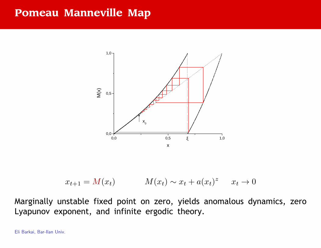
Pomeau Manneville Map

0 , 0 0 , 5 1 , 00 , 0

0 , 5

1 , 0

M(x)

xξ

x 0

xt+1 = M(xt) M(xt) ∼ xt + a(xt)z xt → 0

Marginally unstable fixed point on zero, yields anomalous dynamics, zeroLyapunov exponent, and infinite ergodic theory.


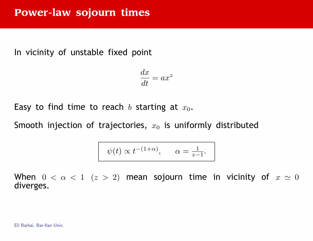
Power-law sojourn times

In vicinity of unstable fixed point

dx

dt= axz

Easy to find time to reach b starting at x0.

Smooth injection of trajectories, x0 is uniformly distributed

ψ(t) ∝ t−(1+α), α = 1z−1.

When 0 < α < 1 (z > 2) mean sojourn time in vicinity of x ' 0diverges.


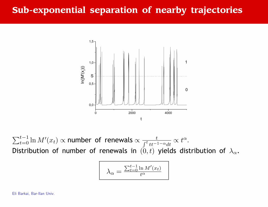
Sub-exponential separation of nearby trajectories

0 2000 4000

0,0

0,5

1,0

1,5

1

ln(|M

'(xt)|)

t

S

0

∑t−1t=0 lnM ′(xt) ∝ number of renewals ∝ t∫ t

tt−1−αdt∝ tα.

Distribution of number of renewals in (0, t) yields distribution of λα.

λα =∑t−1t=0 lnM ′(xt)

tα


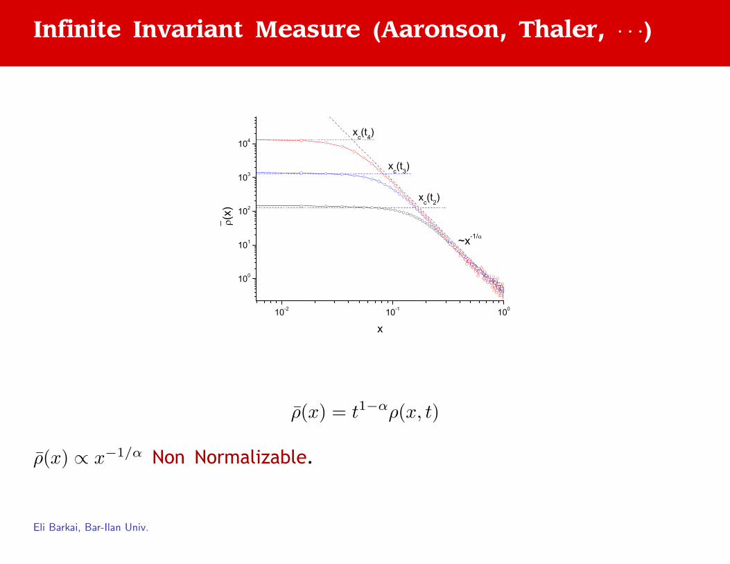
Infinite Invariant Measure (Aaronson, Thaler, · · ·)

10-2 10-1 100

100

101

102

103

104

xc(t3)

xc(t4)

(x)

x

xc(t2)

~x-1/

ρ(x) = t1−αρ(x, t)

ρ(x) ∝ x−1/α Non Normalizable.


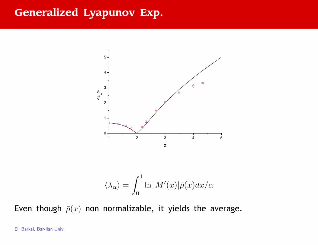
Generalized Lyapunov Exp.

1 2 3 4 50

1

2

3

4

5

<>

z

〈λα〉 =

∫ 1

0

ln |M ′(x)|ρ(x)dx/α

Even though ρ(x) non normalizable, it yields the average.


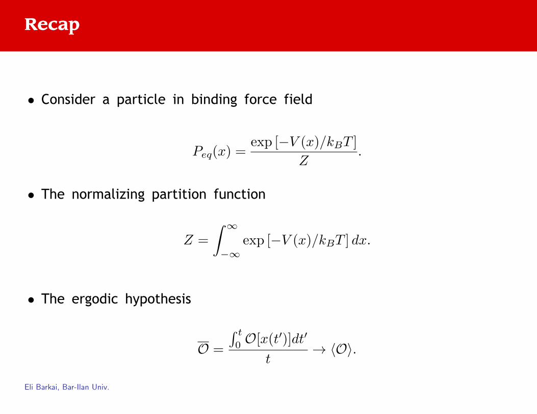
Recap

• Consider a particle in binding force field

Peq(x) =exp [−V (x)/kBT ]

Z.

• The normalizing partition function

Z =

∫ ∞−∞

exp [−V (x)/kBT ] dx.

• The ergodic hypothesis

O =

∫ t0O[x(t′)]dt′

t→ 〈O〉.


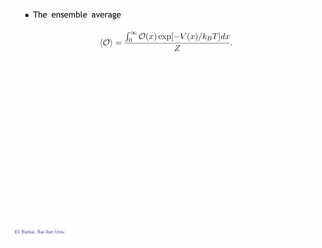
• The ensemble average

〈O〉 =

∫∞0O(x) exp[−V (x)/kBT ]dx

Z.


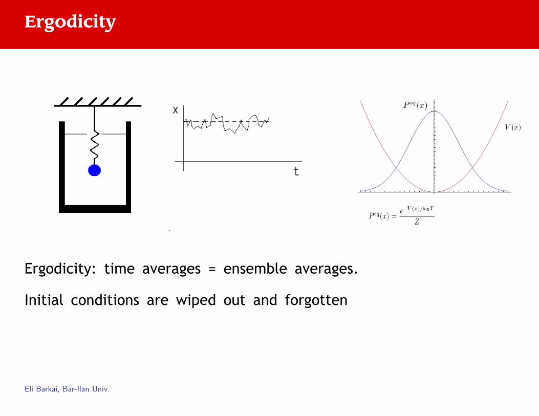
Ergodicity

Ergodicity: time averages = ensemble averages.

Initial conditions are wiped out and forgotten


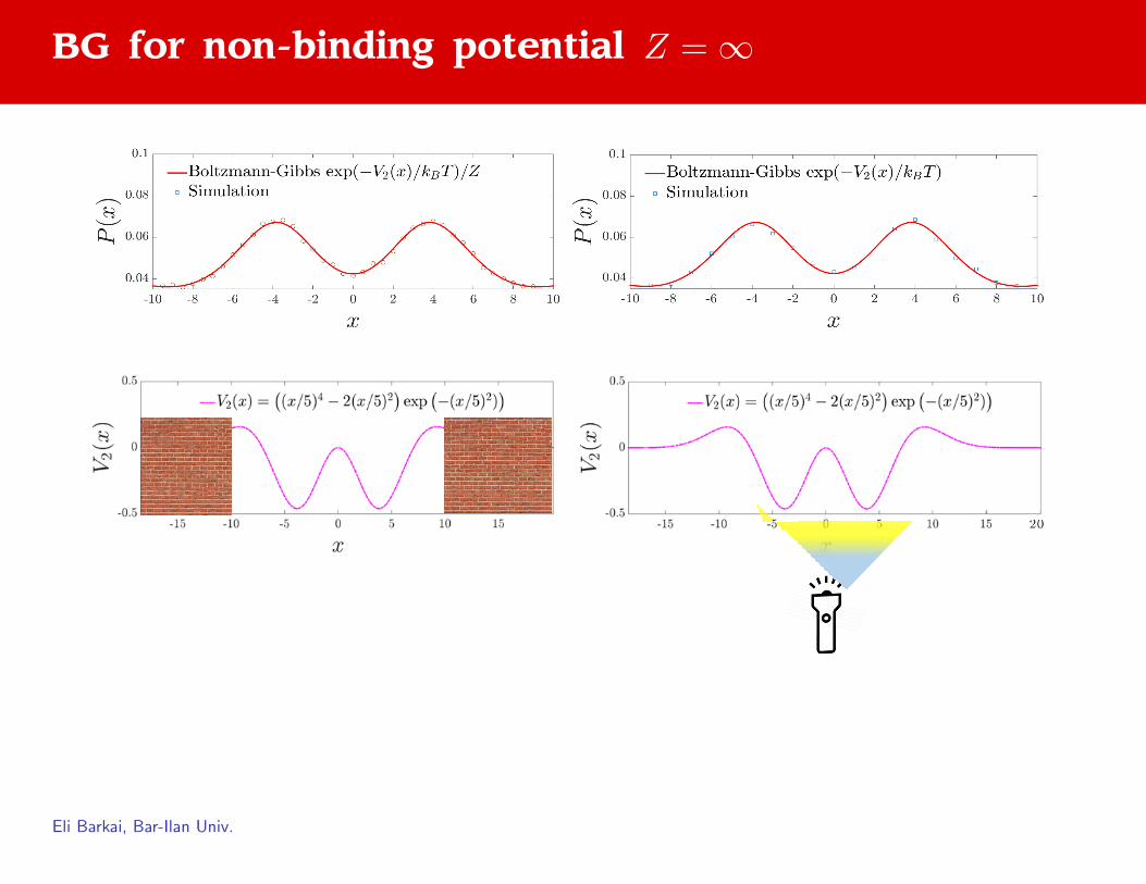
BG for non-binding potential Z =∞


The Hydrogen Paradox (Herzfeld, Fowler, Wigner,...)

The barometric formula ρ(x) = ρ0 exp(−mgh/kBT ) means that we teachstudents that earth is flat. Same problems for black holes.


Non-normalizable

• Bouchuad trap model for glass dynamics

Z ∝∫ ∞

0

exp(−E/Tg + E/T )dE =∞.

• The log potential.

• In physics:A trick is to introduce cutoffs, consider a box philosophy.

• In math:Infinite ergodic theory: Aaronson, Thaler, Zweimuller has an elegant appeal.


Single Molecule Experiments

Particle immersed in a bath with temperature T .Force field vanishes for large x.


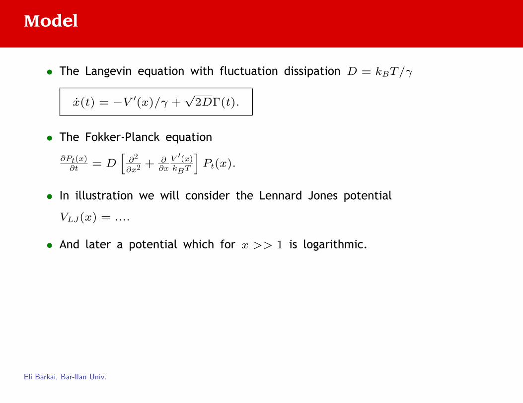
Model

• The Langevin equation with fluctuation dissipation D = kBT/γ

x(t) = −V ′(x)/γ +√

2DΓ(t).

• The Fokker-Planck equation

∂Pt(x)∂t = D

[∂2

∂x2 + ∂∂x

V ′(x)kBT

]Pt(x).

• In illustration we will consider the Lennard Jones potential

VLJ(x) = ....

• And later a potential which for x >> 1 is logarithmic.


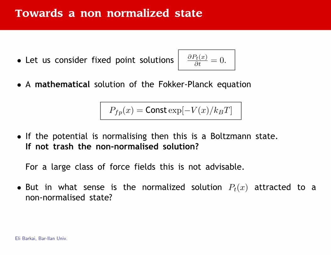
Towards a non normalized state

• Let us consider fixed point solutions ∂Pt(x)∂t = 0.

• A mathematical solution of the Fokker-Planck equation

Pfp(x) = Const exp[−V (x)/kBT ]

• If the potential is normalising then this is a Boltzmann state.If not trash the non-normalised solution?

For a large class of force fields this is not advisable.

• But in what sense is the normalized solution Pt(x) attracted to anon-normalised state?


Normalizable and non-Normalizable fields


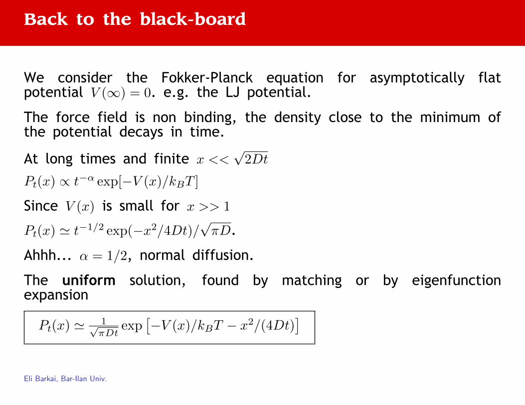
Back to the black-board

We consider the Fokker-Planck equation for asymptotically flatpotential V (∞) = 0. e.g. the LJ potential.

The force field is non binding, the density close to the minimum ofthe potential decays in time.

At long times and finite x <<√

2Dt

Pt(x) ∝ t−α exp[−V (x)/kBT ]

Since V (x) is small for x >> 1

Pt(x) ' t−1/2 exp(−x2/4Dt)/√πD.

Ahhh... α = 1/2, normal diffusion.

The uniform solution, found by matching or by eigenfunctionexpansion

Pt(x) ' 1√πDt

exp[−V (x)/kBT − x2/(4Dt)

]Eli Barkai, Bar-Ilan Univ.

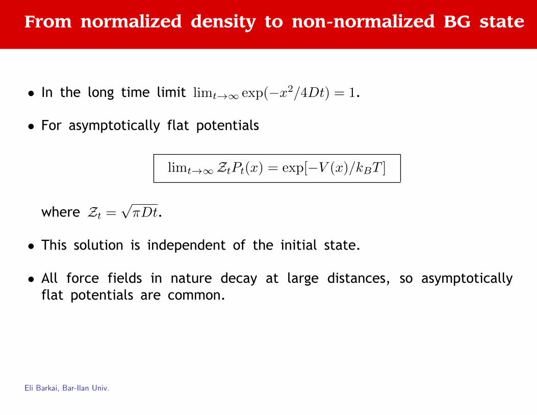
From normalized density to non-normalized BG state

• In the long time limit limt→∞ exp(−x2/4Dt) = 1.

• For asymptotically flat potentials

limt→∞ZtPt(x) = exp[−V (x)/kBT ]

where Zt =√πDt.

• This solution is independent of the initial state.

• All force fields in nature decay at large distances, so asymptoticallyflat potentials are common.


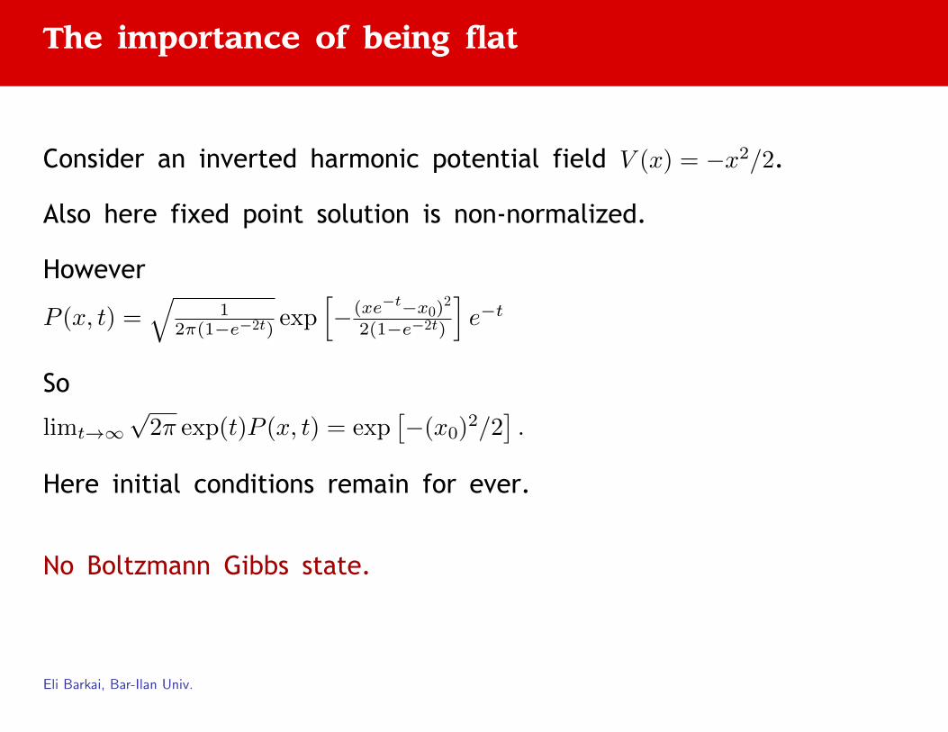
The importance of being flat

Consider an inverted harmonic potential field V (x) = −x2/2.

Also here fixed point solution is non-normalized.

However

P (x, t) =√

12π(1−e−2t)

exp[−(xe−t−x0)

2

2(1−e−2t)

]e−t

So

limt→∞√

2π exp(t)P (x, t) = exp[−(x0)2/2

].

Here initial conditions remain for ever.

No Boltzmann Gibbs state.


Ensemble averages

• The ensemble average, by definition

〈O(x)〉t =∫∞

0O(x)Pt(x)dx.

• In the long time limit,

〈O(x)〉t ∼ 1Zt

∫∞0O(x)e−V (x)/kBTdx.

• Similar to ordinary stat. mech. averages are obtained with respect to theBoltzmann factor.

• Provided that the integral is finite. And then O is called integrable.

• One example is the potential energy of the particles, Ep = V (x).

• Integrable observables are the super common, for example the occupationfraction (also entropy, virial theorem, need non-normalizable stat. mech.).

• We can treat also the non-integrable observables, e.g. O = x2.


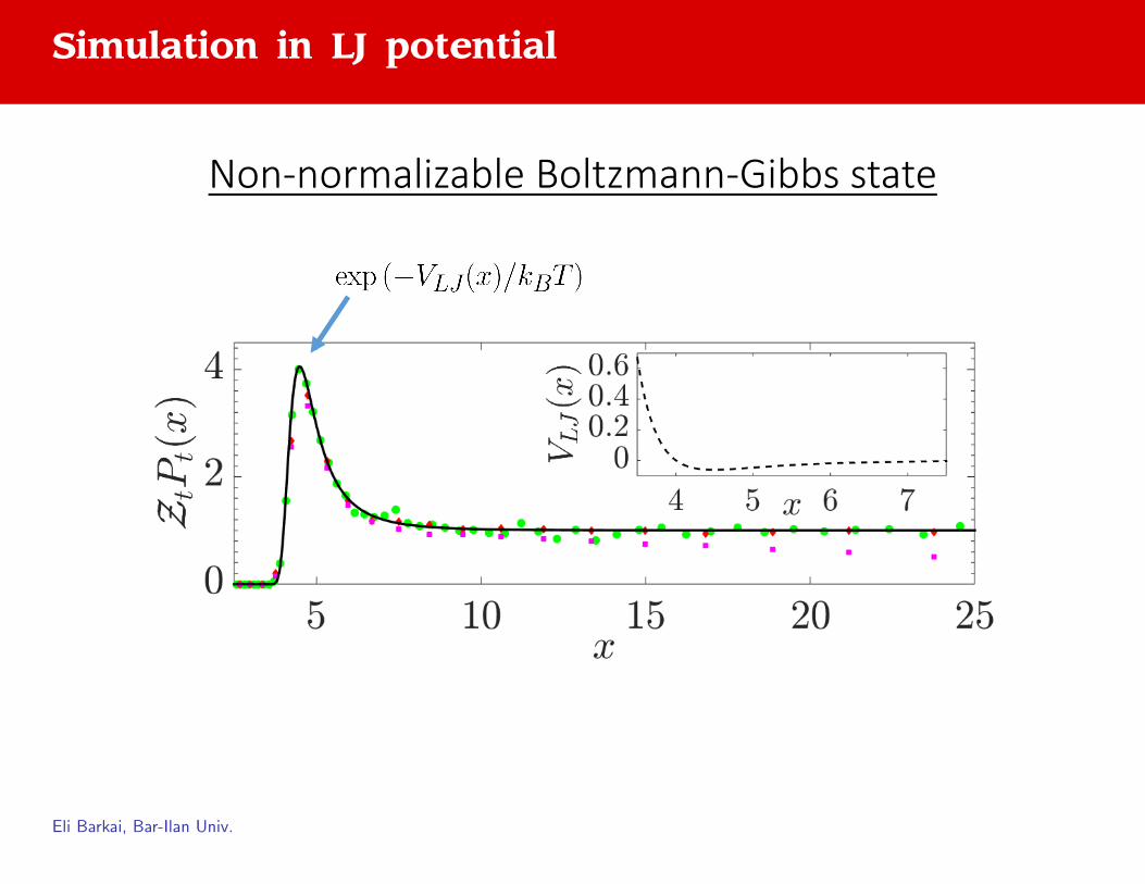
Simulation in LJ potential

Non-normalizable Boltzmann-Gibbs state


Time averages

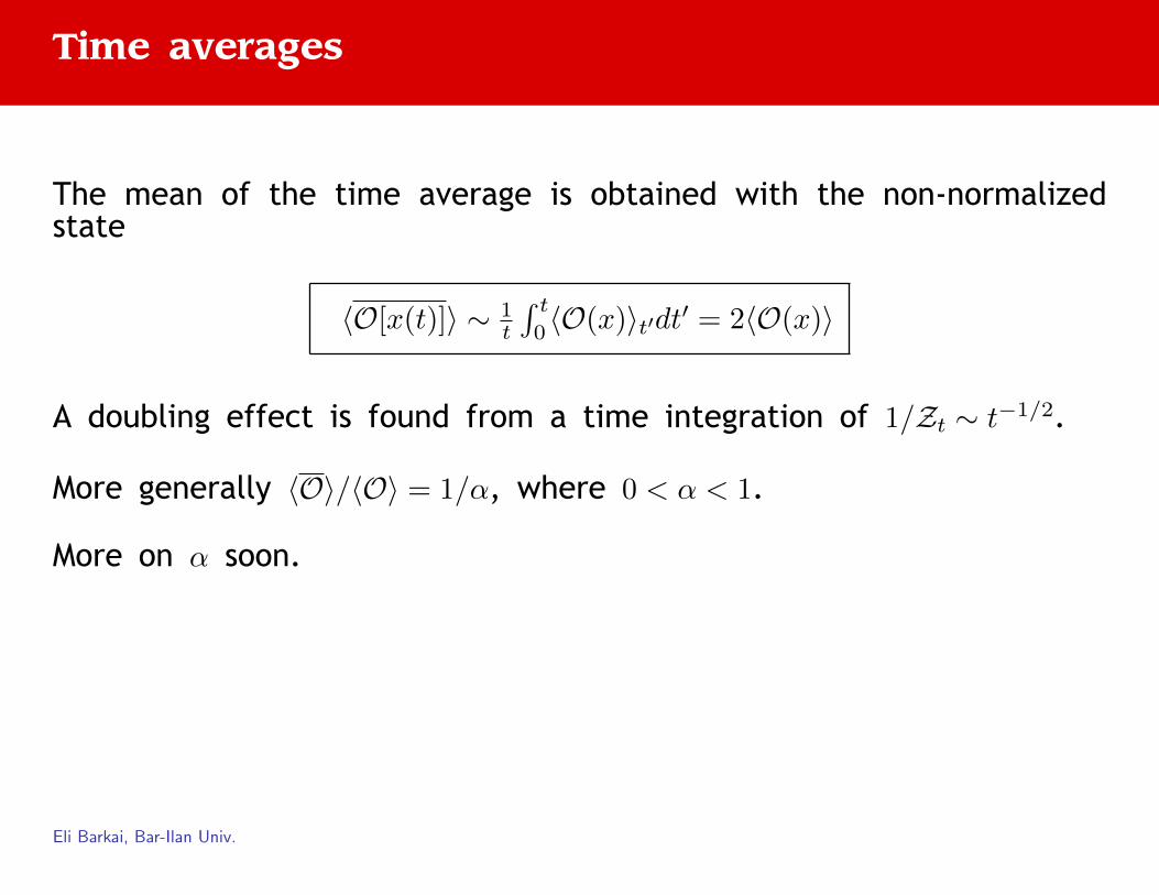
The mean of the time average is obtained with the non-normalizedstate

〈O[x(t)]〉 ∼ 1t

∫ t0〈O(x)〉t′dt′ = 2〈O(x)〉

A doubling effect is found from a time integration of 1/Zt ∼ t−1/2.

More generally 〈O〉/〈O〉 = 1/α, where 0 < α < 1.

More on α soon.


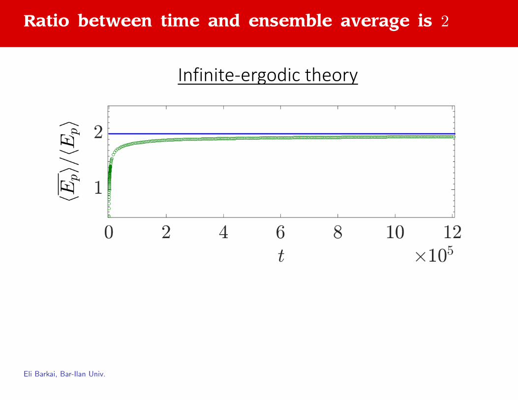
Ratio between time and ensemble average is 2

Infinite-ergodic theory


Entropy extremum principle

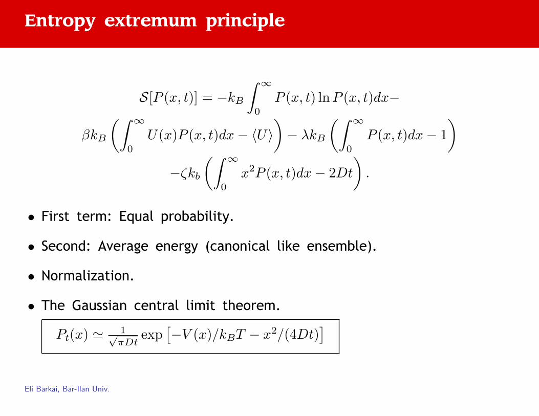
S[P (x, t)] = −kB∫ ∞

0

P (x, t) lnP (x, t)dx−

βkB

(∫ ∞0

U(x)P (x, t)dx− 〈U〉)− λkB

(∫ ∞0

P (x, t)dx− 1

)−ζkb

(∫ ∞0

x2P (x, t)dx− 2Dt

).

• First term: Equal probability.

• Second: Average energy (canonical like ensemble).

• Normalization.

• The Gaussian central limit theorem.

Pt(x) ' 1√πDt

exp[−V (x)/kBT − x2/(4Dt)


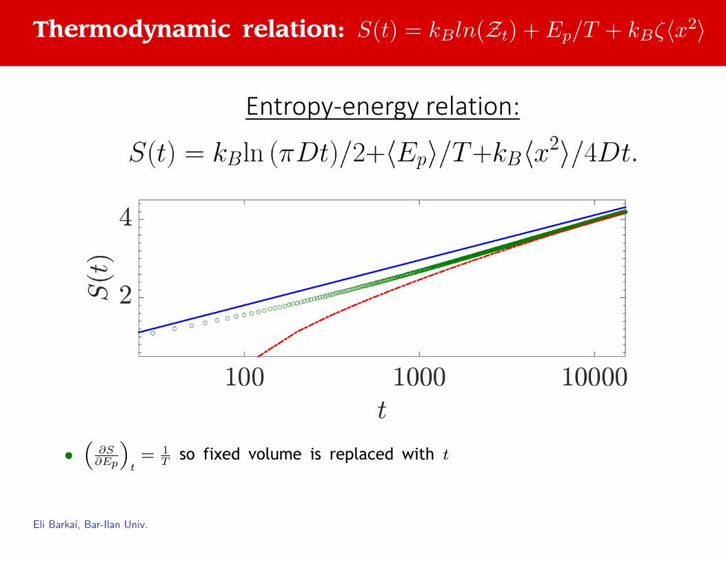
Thermodynamic relation: S(t) = kBln(Zt) + Ep/T + kBζ〈x2〉

Entropy-energy relation:

•(∂S∂Ep

)t

= 1T so fixed volume is replaced with t


Distribution of time average

• Time averages remain random even in the long time limit.

• Let ξ = O/〈O〉.

• For example consider the indicator θ(xa < x(t) < xb) = 1 if condition holds,otherwise zero.

• The sequence 1, 0, 1, 0, , ... with τin, τout, τin, ....

PDF(τout) ∝ (τout)−(1+α)

• α is the first return exponent.

• Mean return time diverges.

• The process is recurrent.

• α = 1/2 for asymptotically flat potentials in dimension one.


Aaronson-Darling-Kac in a thermal setting

Then ξ = O/〈O〉 = n/〈n〉.

The number of events 1 yield the statistics of the time averages.

The time in the interval (xa, xb) is n〈τin〉.

How do we get the PDF of n? First fix n and let t =∑ni τout(i). Here

PDF of t is a one sided Lévy distribution.

Lévy statistics describes the distribution of the timeaverage

The magic: this holds true for any integrable observable.

PDF(ξ) = Γ1/α(1+α)

αξ1+1/α Lα

[Γ1/α(1+α)

αξ1/α


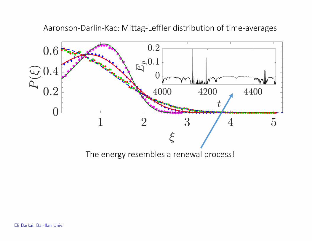
Aaronson-Darlin-Kac: Mittag-Leffler distribution of time-averages

The energy resembles a renewal process!


Distribution of generalized Lyapunov Exp.

ζ = λα/〈λα〉.Renewal Theory: distribution of λα is Mittag-Leffler.Aaronson-Darling-Kac Theorem.Korabel Barkai Phys. Rev. Lett. 102, 050601 (2009).


Particle in a log potential

X0

• V (x) = 0.5 ln(1 + x2), PBG(x) = (1 + x2)−1/2T/Z for T < 1.

• The normal BG phase Kessler Barkai PRL 2010.

• Transition point T = 1.


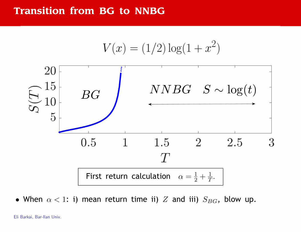
Transition from BG to NNBG

First return calculation α = 12 + 1

T .

• When α < 1: i) mean return time ii) Z and iii) SBG, blow up.


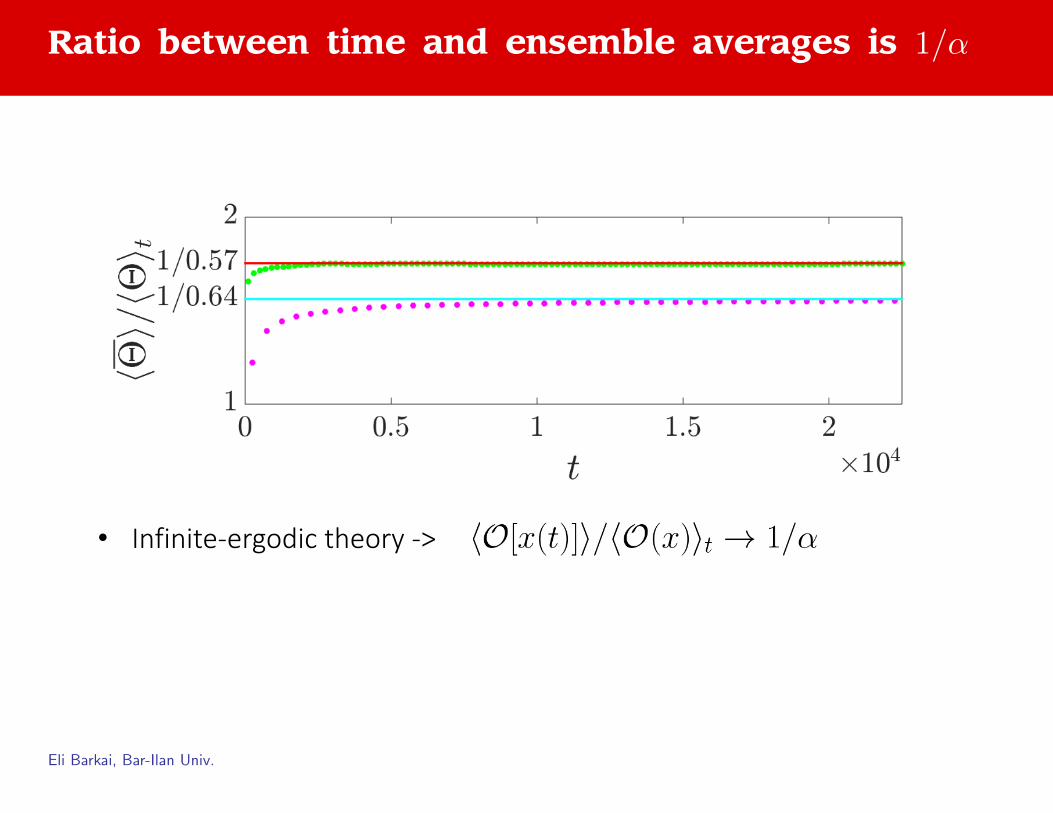
Ratio between time and ensemble averages is 1/α

• Infinite-ergodic theory ->


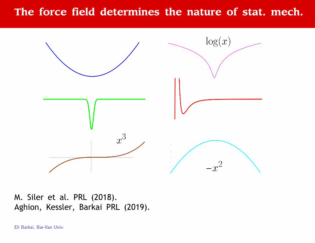
The force field determines the nature of stat. mech.

M. Siler et al. PRL (2018).Aghion, Kessler, Barkai PRL (2019).


Virial Theorem (flat potentials)

• The machinery of stat. mech. can be extended to infinite ergodic theory.

• The virial theorem:

〈xF (x)〉 ∼ 2B2ZtkBT

• B2/Zt ratio of two length scales, with B2 = 12

∫∞0{1− exp[−V (x)/kBT ]} dx.

• Use 〈xF (x)〉 = kBT∫∞

0x∂x[exp(−V (x)/kBT )− 1]dx/Zt.

• B2 is the second virial coefficient.


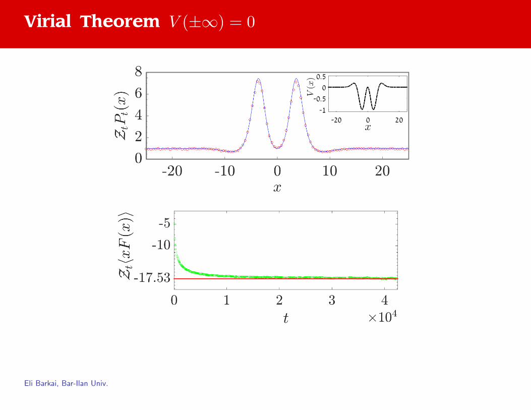
Virial Theorem V (±∞) = 0


Higher dimensions?


Summary

Stochastic thermodynamics of single particle trajectories in thepresence of asymptotically flat (or log) potential fields, uses non-normalised Boltzmann-Gibbs statistics. Both time and ensembleaverages of integrable observables are calculated using the non-normalised Boltzmann state. If the process is recurrent, with aninfinite mean return time, standard ergodic theories obviously fail,however the resampling of the phase space implies that we maystill construct a stat. mech. framework which is independent ofthe initial condition. Lévy statistics describes the fluctuations of thetime averages (ADK theorem). An extremum principle yields a newensemble, where the Gaussian central limit describes the dynamicsfor x >> 1. This leads to non-equilibrium thermodynamic relations,e.g. between entropy and energy.

Aghion, Kessler, Barkai Phys. Rev. Lett. 122, 010601 (2018)


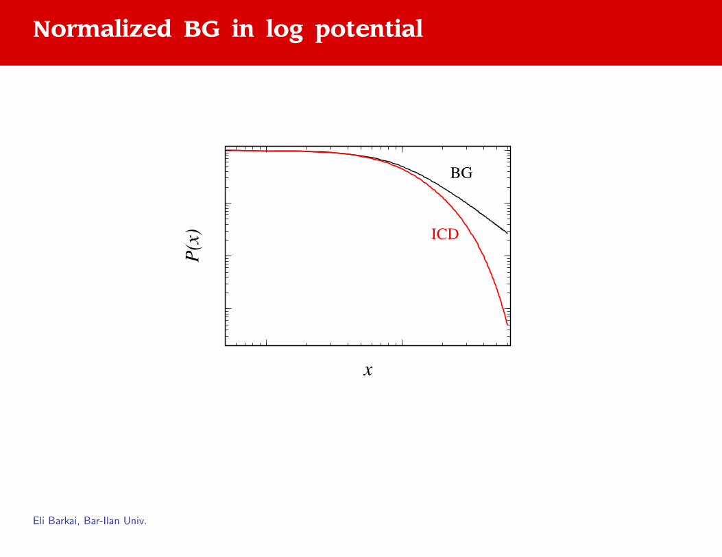
Normalized BG in log potential

x

P(x)

BG

ICD


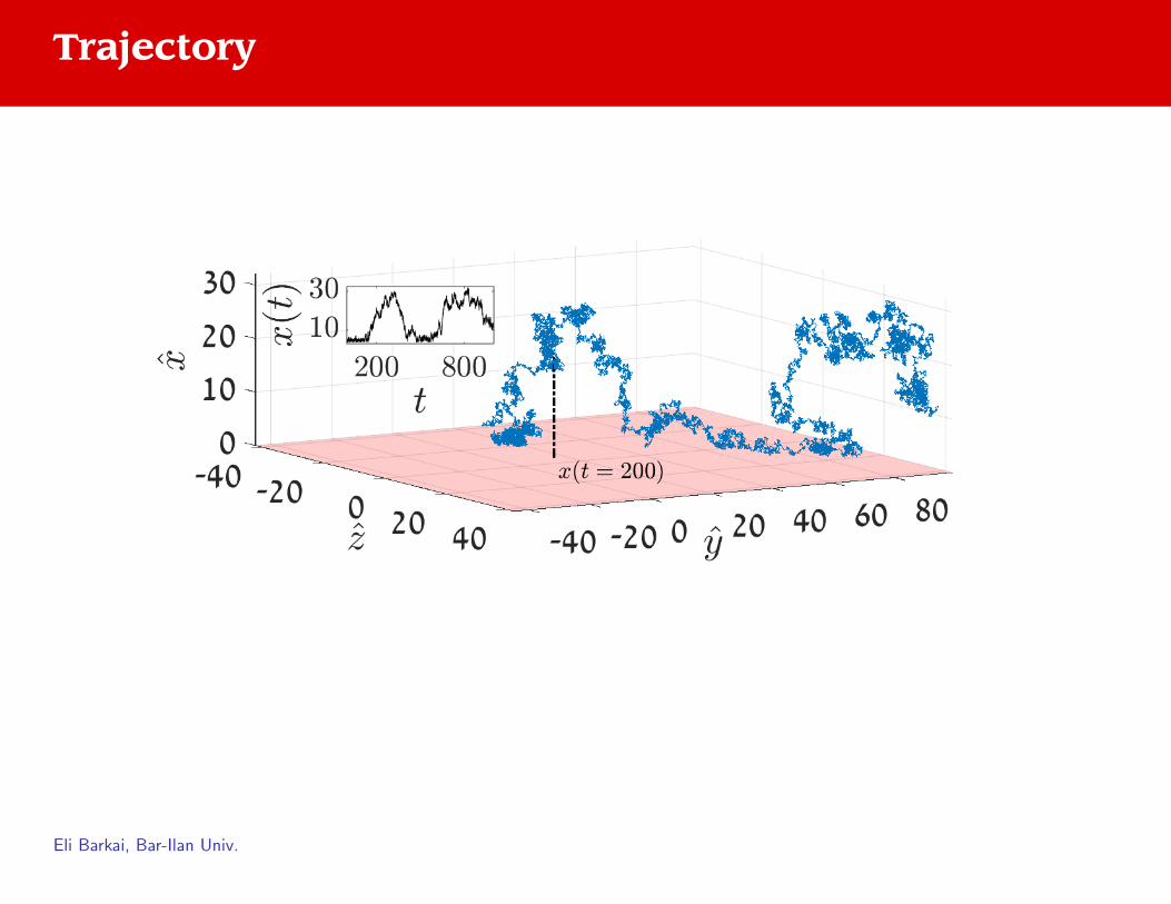
Trajectory


Non-normalized Boltzmann-Gibbs statistics

Documents

Transcript of Non-normalized Boltzmann-Gibbs statistics