μMS³ μModular Substrate Sampling System μMS³ μ Modular Substrate Sampling System.
Advanced Simulation - Lecture 6
George Deligiannidis
February 3rd, 2016
Irreducibility and Recurrence
Proposition
Assume π satisfies the positivity condition, then the Gibbs sampleryields a π−irreducible and recurrent Markov chain.
Proof.Recurrence. Will follow from irreducibility and the fact that πis invariant. Irreducibility. Let X ⊂ Rd, such that π(X) = 1.Write K for the kernel and let A ⊂ X such that π(A) > 0. Thenfor any x ∈ X
K(x, A) =∫
AK(x, y)dy
=∫
AπX1|−1
(y1 | x2, . . . , xd)× · · ·
× πXd|X−d(yd | y1, . . . , yd−1)dy.
Lecture 6 Gibbs Sampling Asymptotics 2 / 1
Proof.Thus if for some x ∈ X and A with π(A) > 0 we haveK(x, A) = 0, we must have that
πX1|X−1(y1 | x2, . . . , xd)× · · · × πXd|X−d(yd | y1, . . . , yd−1) = 0,
for π-almost all y = (y1, . . . , yd) ∈ A.
Therefore we must also have that
π (y1, x2, ..., yd) ∝d
∏j=1
π Xj|X−j
(yj∣∣ y1:j−1, xj+1:d
)π Xj|X−j
(xj∣∣ y1:j−1, xj+1:d
) = 0,
for almost all y = (y1, . . . , yd) ∈ A and thus π(A) = 0 obtaininga contradiction.
Lecture 6 Gibbs Sampling Asymptotics 3 / 1
LLN for Gibbs Sampler
TheoremAssume the positivity condition is satisfied then we have for anyintegrable function ϕ : X→ R:
lim1t
t
∑i=1
ϕ(
X(i))=∫
Xϕ (x)π (x) dx
for π−almost all starting value X(1).
Lecture 6 Gibbs Sampling Asymptotics 4 / 1
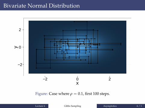
Example: Bivariate Normal Distribution
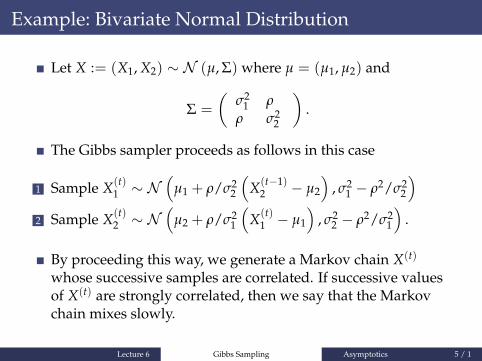
Let X := (X1, X2) ∼ N (µ, Σ) where µ = (µ1, µ2) and
Σ =
(σ2
1 ρρ σ2
2
).
The Gibbs sampler proceeds as follows in this case
1 Sample X(t)1 ∼ N
(µ1 + ρ/σ2
2
(X(t−1)
2 − µ2
), σ2
1 − ρ2/σ22
)2 Sample X(t)
2 ∼ N(
µ2 + ρ/σ21
(X(t)
1 − µ1
), σ2
2 − ρ2/σ21
).
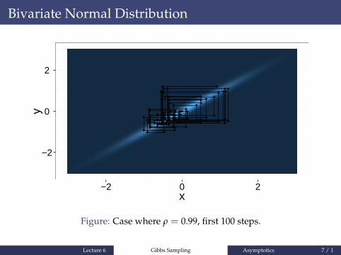
By proceeding this way, we generate a Markov chain X(t)
whose successive samples are correlated. If successive valuesof X(t) are strongly correlated, then we say that the Markovchain mixes slowly.
Lecture 6 Gibbs Sampling Asymptotics 5 / 1
Bivariate Normal Distribution
●●●●
●●
● ●
● ●●●
● ●
●●
● ●
●●
●●
●●
● ●●●
●●
●●
●●
● ●
● ●
● ●
●●
● ●
●●
● ●
● ●
● ●
●●● ●● ●
●●
●●
● ●
● ●
●●
●●
● ●
●●
● ●
●●
● ●● ●●●
● ●
●●
● ●
●●
● ●
● ●
● ●
●●
−2
0
2
−2 0 2x
y
Figure: Case where ρ = 0.1, first 100 steps.
Lecture 6 Gibbs Sampling Asymptotics 6 / 1
Bivariate Normal Distribution
●●
●●
● ●
●●
● ●
●●
● ●
●●
● ●
●●
● ●
●●
● ●
●●
● ●
●●
●●
● ●●●● ●
●●
● ●●●
● ●
●●● ●
●●
● ●
●●
● ●
●●
● ●
●●
● ●
●●
● ●
●●
● ●
●●
● ●
●●
● ●
●●
● ●
●●
● ●
●●
● ●
●●
● ●
−2
0
2
−2 0 2x
y
Figure: Case where ρ = 0.99, first 100 steps.
Lecture 6 Gibbs Sampling Asymptotics 7 / 1
Bivariate Normal Distribution
0.0
0.1
0.2
0.3
0.4
−2 0 2X
dens
ity
(a) Figure A
0.0
0.2
0.4
0.6
−2 0 2X
dens
ity
(b) Figure B
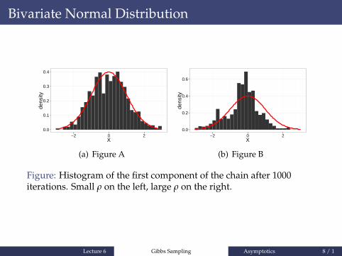
Figure: Histogram of the first component of the chain after 1000iterations. Small ρ on the left, large ρ on the right.
Lecture 6 Gibbs Sampling Asymptotics 8 / 1
Bivariate Normal Distribution
0.0
0.1
0.2
0.3
0.4
−2 0 2X
dens
ity
(a) b
0.0
0.1
0.2
0.3
0.4
−2 0 2X
dens
ity
(b) b
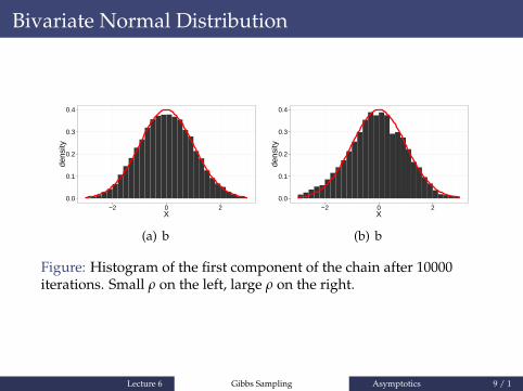
Figure: Histogram of the first component of the chain after 10000iterations. Small ρ on the left, large ρ on the right.
Lecture 6 Gibbs Sampling Asymptotics 9 / 1
Bivariate Normal Distribution
0.0
0.1
0.2
0.3
0.4
−2 0 2X
dens
ity
(a) Figure A
0.0
0.1
0.2
0.3
0.4
−2 0 2X
dens
ity
(b) Figure B
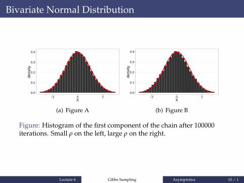
Figure: Histogram of the first component of the chain after 100000iterations. Small ρ on the left, large ρ on the right.
Lecture 6 Gibbs Sampling Asymptotics 10 / 1
Gibbs Sampling and Auxiliary Variables
Gibbs sampling requires sampling from π Xj|X−j.
In many scenarios, we can include a set of auxiliary variablesZ1, ..., Zp and have an “extended” distribution of joint densityπ(
x1, ..., xd, z1, ..., zp)
such that∫π(x1, ..., xd, z1, ..., zp
)dz1...dzd = π (x1, ..., xd) .
which is such that its full conditionals are easy to sample.Mixture models, Capture-recapture models, Tobit models,Probit models etc.
Lecture 6 Gibbs Sampling Asymptotics 11 / 1
Mixtures of Normals
-2 -1 0 1
0.0
0.1
0.2
0.3
0.4
0.5
t
density
mixturepopulation 1population 2population 3
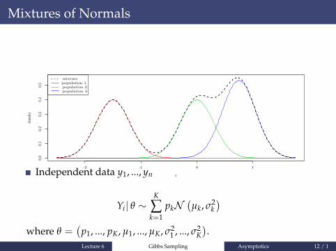
Independent data y1, ..., yn
Yi| θ ∼K
∑k=1
pkN(µk, σ2
k)
where θ =(
p1, ..., pK, µ1, ..., µK, σ21 , ..., σ2
K).
Lecture 6 Gibbs Sampling Asymptotics 12 / 1
Bayesian Model
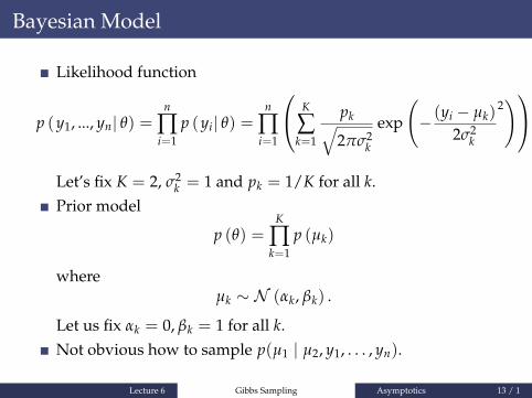
Likelihood function
p (y1, ..., yn| θ) =n
∏i=1
p (yi| θ) =n
∏i=1
K
∑k=1
pk√2πσ2
k
exp
(− (yi − µk)
2σ2k
2) .
Let’s fix K = 2, σ2k = 1 and pk = 1/K for all k.
Prior model
p (θ) =K
∏k=1
p (µk)
whereµk ∼ N (αk, βk) .
Let us fix αk = 0, βk = 1 for all k.Not obvious how to sample p(µ1 | µ2, y1, . . . , yn).
Lecture 6 Gibbs Sampling Asymptotics 13 / 1
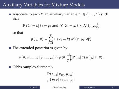
Auxiliary Variables for Mixture Models
Associate to each Yi an auxiliary variable Zi ∈ {1, ..., K} suchthat
P (Zi = k| θ) = pk and Yi| Zi = k, θ ∼ N(µk, σ2
k)
so that
p (yi| θ) =K
∑k=1
P (Zi = k)N(yi; µk, σ2
k)
The extended posterior is given by
p ( θ, z1, ..., zn| y1, ..., yn) ∝ p (θ)n
∏i=1
P ( zi| θ) p (yi| zi, θ) .
Gibbs samples alternately
P( z1:n| y1:n, µ1:K)
p (µ1:K| y1:n, z1:n) .
Lecture 6 Gibbs Sampling Asymptotics 14 / 1
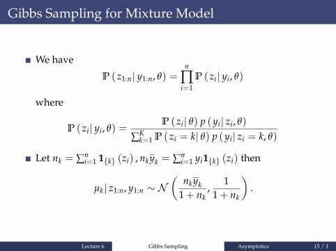
Gibbs Sampling for Mixture Model
We have
P ( z1:n| y1:n, θ) =n
∏i=1
P ( zi| yi, θ)
where
P ( zi| yi, θ) =P ( zi| θ) p (yi| zi, θ)
∑Kk=1 P ( zi = k| θ) p (yi| zi = k, θ)
Let nk = ∑ni=1 1{k} (zi) , nkyk = ∑n
i=1 yi1{k} (zi) then
µk| z1:n, y1:n ∼ N(
nkyk1 + nk
,1
1 + nk
).
Lecture 6 Gibbs Sampling Asymptotics 15 / 1
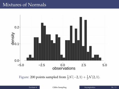
Mixtures of Normals
0.0
0.1
0.2
−5.0 −2.5 0.0 2.5 5.0observations
dens
ity
Figure: 200 points sampled from 12N (−2, 1) + 1
2N (2, 1).
Lecture 6 Gibbs Sampling Asymptotics 16 / 1
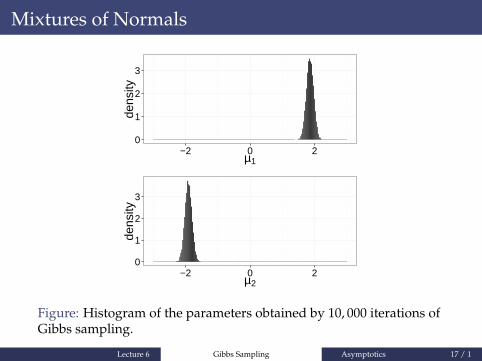
Mixtures of Normals
0
1
2
3
−2 0 2µ1
dens
ity
0
1
2
3
−2 0 2µ2
dens
ity
Figure: Histogram of the parameters obtained by 10, 000 iterations ofGibbs sampling.
Lecture 6 Gibbs Sampling Asymptotics 17 / 1
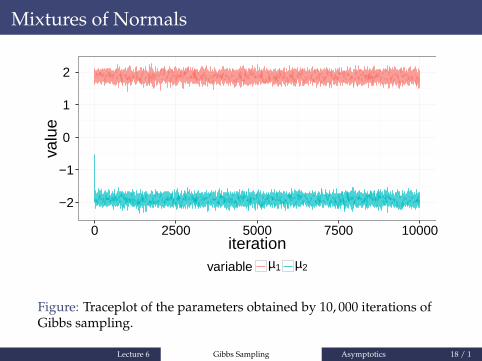
Mixtures of Normals
−2
−1
0
1
2
0 2500 5000 7500 10000iteration
valu
e
variable µ1 µ2
Figure: Traceplot of the parameters obtained by 10, 000 iterations ofGibbs sampling.
Lecture 6 Gibbs Sampling Asymptotics 18 / 1
Gibbs sampling in practice
Many posterior distributions can be automaticallydecomposed into conditional distributions by computerprograms.
This is the idea behind BUGS (Bayesian inference Using GibbsSampling), JAGS (Just another Gibbs Sampler).
Lecture 6 Gibbs Sampling Asymptotics 19 / 1
Outline
Given a target π (x) = π (x1, x2, ..., xd), Gibbs samplingworks by sampling from π Xj|X−j
(xj∣∣ x−j
)for j = 1, ..., d.
Sampling exactly from one of these full conditionals might bea hard problem itself.
Even if it is possible, the Gibbs sampler might convergeslowly if components are highly correlated.
If the components are not highly correlated then Gibbssampling performs well, even when d→ ∞, e.g. with anerror increasing “only” polynomially with d.
Metropolis–Hastings algorithm (1953, 1970) is a more generalalgorithm that can bypass these problems.Additionally Gibbs can be recovered as a special case.
Lecture 6 Gibbs Sampling Asymptotics 20 / 1
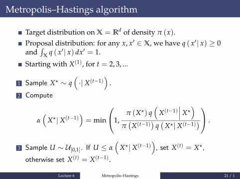
Metropolis–Hastings algorithm
Target distribution on X = Rd of density π (x).Proposal distribution: for any x, x′ ∈ X, we have q ( x′| x) ≥ 0and
∫X
q ( x′| x) dx′ = 1.
Starting with X(1), for t = 2, 3, ...
1 Sample X? ∼ q(·|X(t−1)
).
2 Compute
α(
X?|X(t−1))= min
1,π (X?) q
(X(t−1)
∣∣∣X?)
π(X(t−1)
)q(
X?|X(t−1)) .
3 Sample U ∼ U[0,1]. If U ≤ α(
X?|X(t−1))
, set X(t) = X?,otherwise set X(t) = X(t−1).
Lecture 6 Metropolis–Hastings 21 / 1

Metropolis–Hastings algorithm
●
−2
0
2
−2 0 2x
y
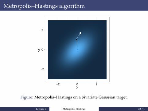
Figure: Metropolis–Hastings on a bivariate Gaussian target.
Lecture 6 Metropolis–Hastings 22 / 1

Metropolis–Hastings algorithm
●●
−2
0
2
−2 0 2x
y
Figure: Metropolis–Hastings on a bivariate Gaussian target.
Lecture 6 Metropolis–Hastings 22 / 1

Metropolis–Hastings algorithm
●
●
−2
0
2
−2 0 2x
y
Figure: Metropolis–Hastings on a bivariate Gaussian target.
Lecture 6 Metropolis–Hastings 22 / 1

Metropolis–Hastings algorithm
●
●●
−2
0
2
−2 0 2x
y
Figure: Metropolis–Hastings on a bivariate Gaussian target.
Lecture 6 Metropolis–Hastings 22 / 1

Metropolis–Hastings algorithm
●●
−2
0
2
−2 0 2x
y
Figure: Metropolis–Hastings on a bivariate Gaussian target.
Lecture 6 Metropolis–Hastings 22 / 1

Metropolis–Hastings algorithm
●●●
−2
0
2
−2 0 2x
y
Figure: Metropolis–Hastings on a bivariate Gaussian target.
Lecture 6 Metropolis–Hastings 22 / 1

Metropolis–Hastings algorithm
●
●
−2
0
2
−2 0 2x
y
Figure: Metropolis–Hastings on a bivariate Gaussian target.
Lecture 6 Metropolis–Hastings 22 / 1

Metropolis–Hastings algorithm
●
●●
−2
0
2
−2 0 2x
y
Figure: Metropolis–Hastings on a bivariate Gaussian target.
Lecture 6 Metropolis–Hastings 22 / 1
Metropolis–Hastings algorithm
●
●
−2
0
2
−2 0 2x
y
Figure: Metropolis–Hastings on a bivariate Gaussian target.
Lecture 6 Metropolis–Hastings 22 / 1

Metropolis–Hastings algorithm
●
●●
−2
0
2
−2 0 2x
y
Figure: Metropolis–Hastings on a bivariate Gaussian target.
Lecture 6 Metropolis–Hastings 22 / 1

Metropolis–Hastings algorithm
●
●
−2
0
2
−2 0 2x
y
Figure: Metropolis–Hastings on a bivariate Gaussian target.
Lecture 6 Metropolis–Hastings 22 / 1

Metropolis–Hastings algorithm
●
●●
−2
0
2
−2 0 2x
y
Figure: Metropolis–Hastings on a bivariate Gaussian target.
Lecture 6 Metropolis–Hastings 22 / 1

Metropolis–Hastings algorithm
●
●
−2
0
2
−2 0 2x
y
Figure: Metropolis–Hastings on a bivariate Gaussian target.
Lecture 6 Metropolis–Hastings 22 / 1

Metropolis–Hastings algorithm
●
●●
−2
0
2
−2 0 2x
y
Figure: Metropolis–Hastings on a bivariate Gaussian target.
Lecture 6 Metropolis–Hastings 22 / 1

Metropolis–Hastings algorithm
●
●
−2
0
2
−2 0 2x
y
Figure: Metropolis–Hastings on a bivariate Gaussian target.
Lecture 6 Metropolis–Hastings 22 / 1

Metropolis–Hastings algorithm
●
●●
−2
0
2
−2 0 2x
y
Figure: Metropolis–Hastings on a bivariate Gaussian target.
Lecture 6 Metropolis–Hastings 22 / 1

Metropolis–Hastings algorithm
●
●
−2
0
2
−2 0 2x
y
Figure: Metropolis–Hastings on a bivariate Gaussian target.
Lecture 6 Metropolis–Hastings 22 / 1

Metropolis–Hastings algorithm
●
●●
−2
0
2
−2 0 2x
y
Figure: Metropolis–Hastings on a bivariate Gaussian target.
Lecture 6 Metropolis–Hastings 22 / 1

Metropolis–Hastings algorithm
●
●
−2
0
2
−2 0 2x
y
Figure: Metropolis–Hastings on a bivariate Gaussian target.
Lecture 6 Metropolis–Hastings 22 / 1

Metropolis–Hastings algorithm
●
●●
−2
0
2
−2 0 2x
y
Figure: Metropolis–Hastings on a bivariate Gaussian target.
Lecture 6 Metropolis–Hastings 22 / 1
Metropolis–Hastings algorithm
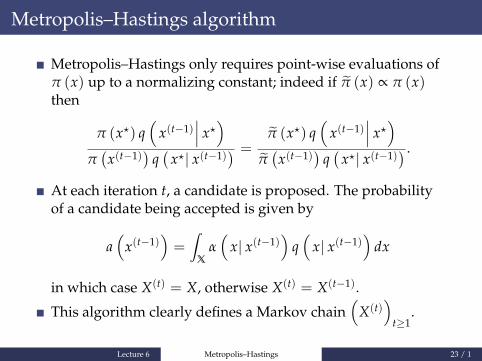
Metropolis–Hastings only requires point-wise evaluations ofπ (x) up to a normalizing constant; indeed if π̃ (x) ∝ π (x)then
π (x?) q(
x(t−1)∣∣∣ x?)
π(
x(t−1))
q(
x?| x(t−1)) =
π̃ (x?) q(
x(t−1)∣∣∣ x?)
π̃(x(t−1)
)q(
x?| x(t−1)) .
At each iteration t, a candidate is proposed. The probabilityof a candidate being accepted is given by
a(
x(t−1))=∫
Xα(
x| x(t−1))
q(
x| x(t−1))
dx
in which case X(t) = X, otherwise X(t) = X(t−1).
This algorithm clearly defines a Markov chain(
X(t))
t≥1.
Lecture 6 Metropolis–Hastings 23 / 1
Transition Kernel and Reversibility
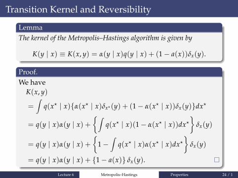
LemmaThe kernel of the Metropolis–Hastings algorithm is given by
K(y | x) ≡ K(x, y) = α(y | x)q(y | x) + (1− a(x))δx(y).
Proof.We have
K(x, y)
=∫
q(x? | x){α(x? | x)δx?(y) + (1− α(x? | x))δx(y)}dx?
= q(y | x)α(y | x) +{∫
q(x? | x)(1− α(x? | x))dx?}
δx(y)
= q(y | x)α(y | x) +{
1−∫
q(x? | x)α(x? | x)dx?}
δx(y)
= q(y | x)α(y | x) + {1− a(x)} δx(y).
Lecture 6 Metropolis–Hastings Properties 24 / 1
Reversibility
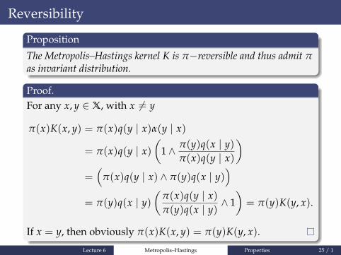
Proposition
The Metropolis–Hastings kernel K is π−reversible and thus admit πas invariant distribution.
Proof.For any x, y ∈ X, with x 6= y
π(x)K(x, y) = π(x)q(y | x)α(y | x)
= π(x)q(y | x)(
1∧ π(y)q(x | y)π(x)q(y | x)
)=(
π(x)q(y | x) ∧ π(y)q(x | y))
= π(y)q(x | y)(
π(x)q(y | x)π(y)q(x | y)
∧ 1)= π(y)K(y, x).
If x = y, then obviously π(x)K(x, y) = π(y)K(y, x).
Lecture 6 Metropolis–Hastings Properties 25 / 1
Reducibility and periodicity of Metropolis–Hastings
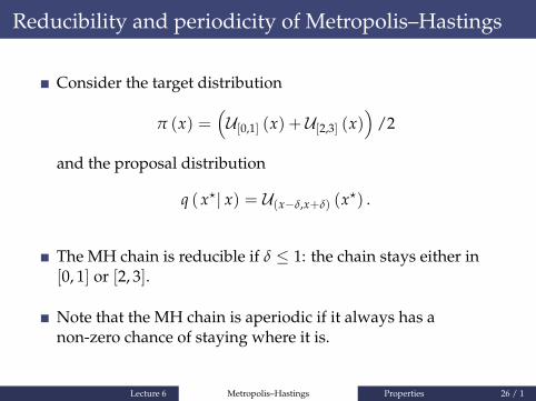
Consider the target distribution
π (x) =(U[0,1] (x) + U[2,3] (x)
)/2
and the proposal distribution
q ( x?| x) = U(x−δ,x+δ) (x?) .
The MH chain is reducible if δ ≤ 1: the chain stays either in[0, 1] or [2, 3].
Note that the MH chain is aperiodic if it always has anon-zero chance of staying where it is.
Lecture 6 Metropolis–Hastings Properties 26 / 1
Some results
Proposition
If q ( x?| x) > 0 for any x, x? ∈ supp(π) then theMetropolis-Hastings chain is irreducible, in fact every state can bereached in a single step (strongly irreducible).
Less strict conditions in (Roberts & Rosenthal, 2004).
Proposition
If the MH chain is irreducible then it is also Harris recurrent(seeTierney, 1994).
Lecture 6 Metropolis–Hastings Properties 27 / 1
LLN for MH
TheoremIf the Markov chain generated by the Metropolis–Hastings sampler isπ−irreducible, then we have for any integrable function ϕ : X→ R:
limt→∞
1t
t
∑i=1
ϕ(
X(i))=∫
Xϕ (x)π (x) dx
for every starting value X(1).
Lecture 6 Metropolis–Hastings Properties 28 / 1

Random Walk Metropolis–Hastings
In the Metropolis–Hastings, pick q(x? | x) = g(x? − x) with gbeing a symmetric distribution, thus
X? = X + ε, ε ∼ g;
e.g. g is a zero-mean multivariate normal or t-student.Acceptance probability becomes
α(x? | x) = min(
1,π(x?)π(x)
).
We accept...
a move to a more probable state with probability 1;a move to a less probable state with probability
π(x?)/π(x) < 1.
Lecture 6 Metropolis–Hastings Properties 29 / 1
Independent Metropolis–Hastings
Independent proposal: a proposal distribution q(x? | x)which does not depend on x.
Acceptance probability becomes
α(x? | x) = min(
1,π(x?)q(x)π(x)q(x?)
).
For instance, multivariate normal or t-studentdistribution.
If π(x)/q(x) < M for all x and some M < ∞, then the chainis uniformly ergodic.The acceptance probability at stationarity is at least 1/M(Lemma 7.9 of Robert & Casella).On the other hand, if such an M does not exist, the chain isnot even geometrically ergodic!
Lecture 6 Metropolis–Hastings Independent MH 30 / 1
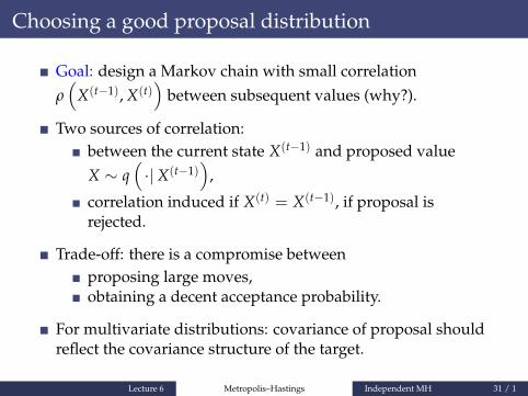
Choosing a good proposal distribution
Goal: design a Markov chain with small correlationρ(
X(t−1), X(t))
between subsequent values (why?).
Two sources of correlation:between the current state X(t−1) and proposed valueX ∼ q
(·|X(t−1)
),
correlation induced if X(t) = X(t−1), if proposal isrejected.
Trade-off: there is a compromise betweenproposing large moves,obtaining a decent acceptance probability.
For multivariate distributions: covariance of proposal shouldreflect the covariance structure of the target.
Lecture 6 Metropolis–Hastings Independent MH 31 / 1
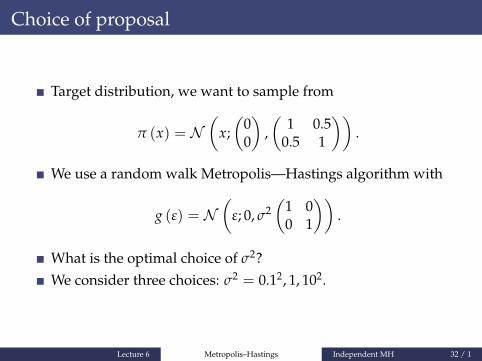
Choice of proposal
Target distribution, we want to sample from
π (x) = N(
x;(
00
),(
1 0.50.5 1
)).
We use a random walk Metropolis—Hastings algorithm with
g (ε) = N(
ε; 0, σ2(
1 00 1
)).
What is the optimal choice of σ2?We consider three choices: σ2 = 0.12, 1, 102.
Lecture 6 Metropolis–Hastings Independent MH 32 / 1
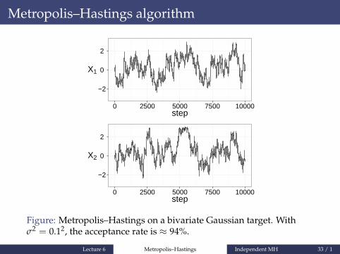
Metropolis–Hastings algorithm
−2
0
2
0 2500 5000 7500 10000step
X1
−2
0
2
0 2500 5000 7500 10000step
X2
Figure: Metropolis–Hastings on a bivariate Gaussian target. Withσ2 = 0.12, the acceptance rate is ≈ 94%.
Lecture 6 Metropolis–Hastings Independent MH 33 / 1
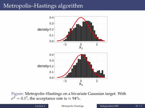
Metropolis–Hastings algorithm
0.0
0.1
0.2
0.3
0.4
−2 0 2X1
density
0.0
0.1
0.2
0.3
0.4
−2 0 2X2
density
Figure: Metropolis–Hastings on a bivariate Gaussian target. Withσ2 = 0.12, the acceptance rate is ≈ 94%.
Lecture 6 Metropolis–Hastings Independent MH 33 / 1
Metropolis–Hastings algorithm
−2
0
2
0 2500 5000 7500 10000step
X1
−2
0
2
0 2500 5000 7500 10000step
X2
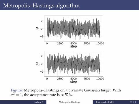
Figure: Metropolis–Hastings on a bivariate Gaussian target. Withσ2 = 1, the acceptance rate is ≈ 52%.
Lecture 6 Metropolis–Hastings Independent MH 33 / 1
Metropolis–Hastings algorithm
0.0
0.1
0.2
0.3
0.4
−2 0 2X1
density
0.0
0.1
0.2
0.3
0.4
−2 0 2X2
density
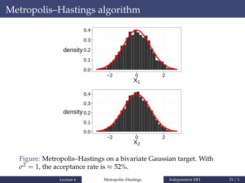
Figure: Metropolis–Hastings on a bivariate Gaussian target. Withσ2 = 1, the acceptance rate is ≈ 52%.
Lecture 6 Metropolis–Hastings Independent MH 33 / 1
Metropolis–Hastings algorithm
−2
0
2
0 2500 5000 7500 10000step
X1
−2
0
2
0 2500 5000 7500 10000step
X2
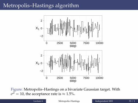
Figure: Metropolis–Hastings on a bivariate Gaussian target. Withσ2 = 10, the acceptance rate is ≈ 1.5%.
Lecture 6 Metropolis–Hastings Independent MH 33 / 1
Metropolis–Hastings algorithm
0.0
0.2
0.4
0.6
−2 0 2X1
density
0.0
0.2
0.4
0.6
0.8
−2 0 2X2
density
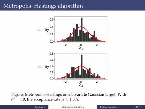
Figure: Metropolis–Hastings on a bivariate Gaussian target. Withσ2 = 10, the acceptance rate is ≈ 1.5%.
Lecture 6 Metropolis–Hastings Independent MH 33 / 1
Choice of proposal
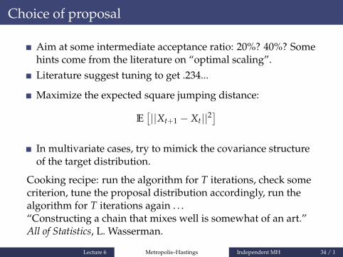
Aim at some intermediate acceptance ratio: 20%? 40%? Somehints come from the literature on “optimal scaling”.Literature suggest tuning to get .234...
Maximize the expected square jumping distance:
E[||Xt+1 − Xt||2
]In multivariate cases, try to mimick the covariance structureof the target distribution.
Cooking recipe: run the algorithm for T iterations, check somecriterion, tune the proposal distribution accordingly, run thealgorithm for T iterations again . . .“Constructing a chain that mixes well is somewhat of an art.”All of Statistics, L. Wasserman.
Lecture 6 Metropolis–Hastings Independent MH 34 / 1
The adaptive MCMC approach
One can make the transition kernel K adaptive, i.e. use Kt atiteration t and choose Kt using the past sample(X1, . . . , Xt−1).
The Markov chain is not homogeneous anymore: themathematical study of the algorithm is much morecomplicated.
Adaptation can be counterproductive in some cases (seeAtchadé & Rosenthal, 2005)!
Adaptive Gibbs samplers also exist.
Lecture 6 Metropolis–Hastings Independent MH 35 / 1