
More on the New Keynesian Model - SSCC - Home
52
More on the New Keynesian Model Noah Williams University of Wisconsin-Madison Noah Williams (UW Madison) New Keynesian model 1 / 52
Transcript of More on the New Keynesian Model - SSCC - Home

More on the New Keynesian Model
Noah Williams
University of Wisconsin-Madison
Noah Williams (UW Madison) New Keynesian model 1 / 52
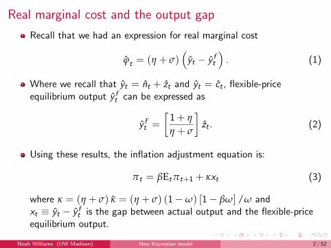
Real marginal cost and the output gap
Recall that we had an expression for real marginal cost
ϕt = (η + σ)(yt − y ft
). (1)
Where we recall that yt = nt + zt and yt = ct , flexible-priceequilibrium output y ft can be expressed as
y ft =
[1 + η
η + σ
]zt . (2)
Using these results, the inflation adjustment equation is:
πt = βEtπt+1 + κxt (3)
where κ = (η + σ) κ = (η + σ) (1−ω) [1− βω] /ω andxt ≡ yt − y ft is the gap between actual output and the flexible-priceequilibrium output.
Noah Williams (UW Madison) New Keynesian model 2 / 52
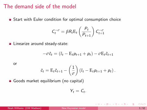
The demand side of the model
Start with Euler condition for optimal consumption choice
C−σt = βRtEt
(Pt
Pt+1
)C−σt+1
Linearize around steady-state:
−σct = (ıt − Etpt+1 + pt)− σEt ct+1
or
ct = Et ct+1 −(
1
σ
)(ıt − Etpt+1 + pt) .
Goods market equilibrium (no capital)
Yt = Ct .
Noah Williams (UW Madison) New Keynesian model 3 / 52
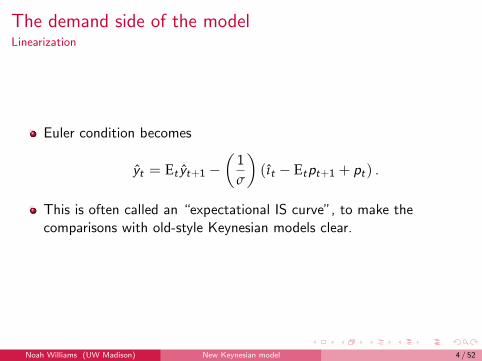
The demand side of the modelLinearization
Euler condition becomes
yt = Et yt+1 −(
1
σ
)(ıt − Etpt+1 + pt) .
This is often called an “expectational IS curve”, to make thecomparisons with old-style Keynesian models clear.
Noah Williams (UW Madison) New Keynesian model 4 / 52
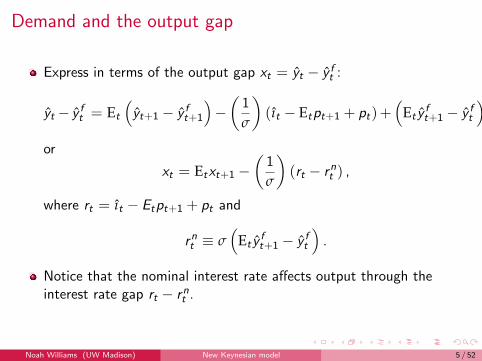
Demand and the output gap
Express in terms of the output gap xt = yt − y ft :
yt − y ft = Et
(yt+1 − y ft+1
)−(
1
σ
)(ıt − Etpt+1 + pt)+
(Et y
ft+1 − y ft
),
or
xt = Etxt+1 −(
1
σ
)(rt − rnt ) ,
where rt = ıt − Etpt+1 + pt and
rnt ≡ σ(
Et yft+1 − y ft
).
Notice that the nominal interest rate affects output through theinterest rate gap rt − rnt .
Noah Williams (UW Madison) New Keynesian model 5 / 52
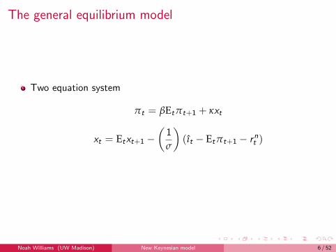
The general equilibrium model
Two equation system
πt = βEtπt+1 + κxt
xt = Etxt+1 −(
1
σ
)(ıt − Etπt+1 − rnt )
Noah Williams (UW Madison) New Keynesian model 6 / 52
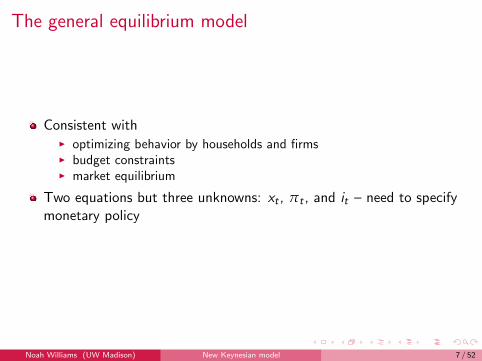
The general equilibrium model
Consistent withI optimizing behavior by households and firmsI budget constraintsI market equilibrium
Two equations but three unknowns: xt , πt , and it – need to specifymonetary policy
Noah Williams (UW Madison) New Keynesian model 7 / 52
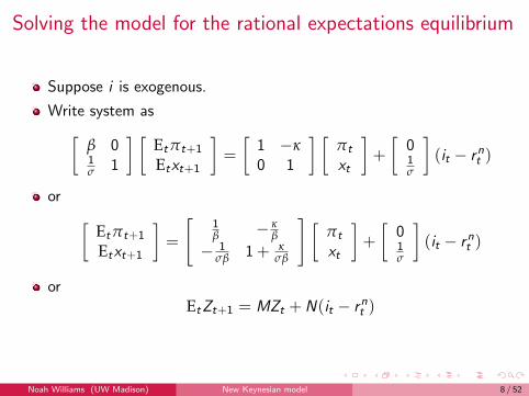
Solving the model for the rational expectations equilibrium
Suppose i is exogenous.
Write system as[β 01σ 1
] [Etπt+1
Etxt+1
]=
[1 −κ0 1
] [πt
xt
]+
[01σ
](it − rnt )
or [Etπt+1
Etxt+1
]=
[1β − κ
β
− 1σβ 1 + κ
σβ
] [πt
xt
]+
[01σ
](it − rnt )
orEtZt+1 = MZt +N(it − rnt )
Noah Williams (UW Madison) New Keynesian model 8 / 52
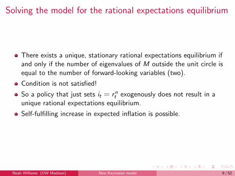
Solving the model for the rational expectations equilibrium
There exists a unique, stationary rational expectations equilibrium ifand only if the number of eigenvalues of M outside the unit circle isequal to the number of forward-looking variables (two).
Condition is not satisfied!
So a policy that just sets it = rnt exogenously does not result in aunique rational expectations equilibrium.
Self-fulfilling increase in expected inflation is possible.
Noah Williams (UW Madison) New Keynesian model 9 / 52
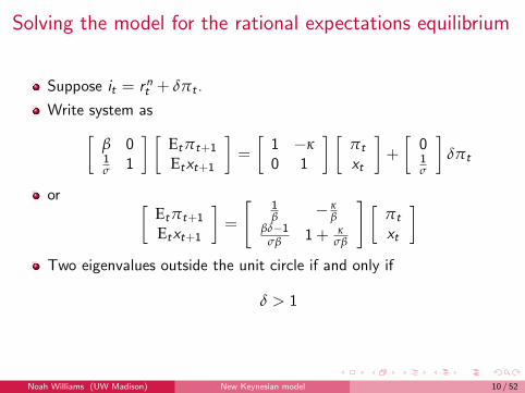
Solving the model for the rational expectations equilibrium
Suppose it = rnt + δπt .
Write system as[β 01σ 1
] [Etπt+1
Etxt+1
]=
[1 −κ0 1
] [πt
xt
]+
[01σ
]δπt
or [Etπt+1
Etxt+1
]=
[1β − κ
ββδ−1
σβ 1 + κσβ
] [πt
xt
]Two eigenvalues outside the unit circle if and only if
δ > 1
Noah Williams (UW Madison) New Keynesian model 10 / 52
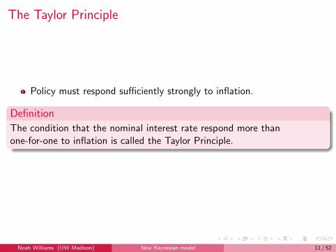
The Taylor Principle
Policy must respond sufficiently strongly to inflation.
Definition
The condition that the nominal interest rate respond more thanone-for-one to inflation is called the Taylor Principle.
Noah Williams (UW Madison) New Keynesian model 11 / 52
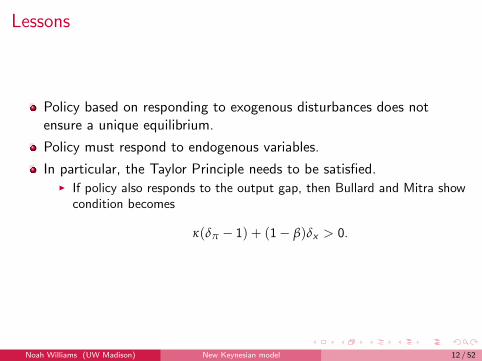
Lessons
Policy based on responding to exogenous disturbances does notensure a unique equilibrium.
Policy must respond to endogenous variables.
In particular, the Taylor Principle needs to be satisfied.I If policy also responds to the output gap, then Bullard and Mitra show
condition becomes
κ(δπ − 1) + (1− β)δx > 0.
Noah Williams (UW Madison) New Keynesian model 12 / 52
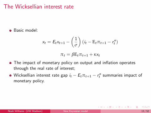
The Wicksellian interest rate
Basic model:
xt = Etxt+1 −(
1
σ
)(it − Etπt+1 − rnt )
πt = βEtπt+1 + κxt
The impact of monetary policy on output and inflation operatesthrough the real rate of interest;
Wicksellian interest rate gap it − Etπt+1 − rnt summaries impact ofmonetary policy.
Noah Williams (UW Madison) New Keynesian model 13 / 52
The Wicksellian interest rate
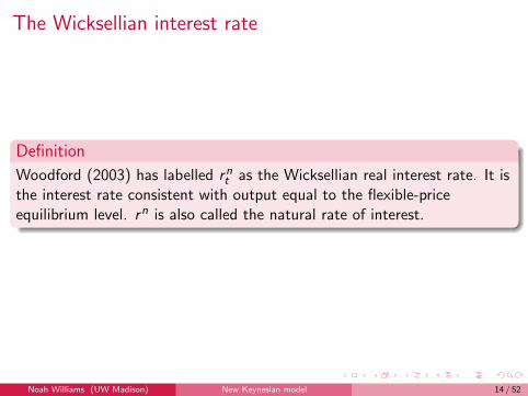
Definition
Woodford (2003) has labelled rnt as the Wicksellian real interest rate. It isthe interest rate consistent with output equal to the flexible-priceequilibrium level. rn is also called the natural rate of interest.
Noah Williams (UW Madison) New Keynesian model 14 / 52
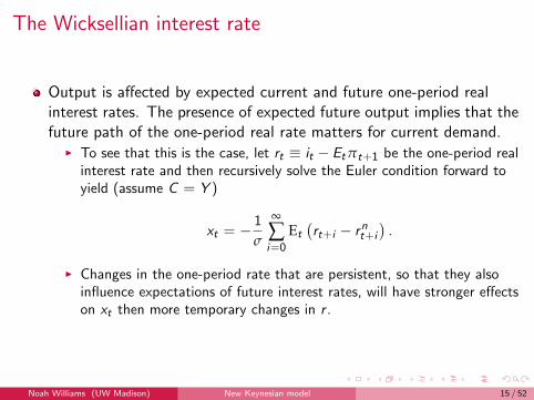
The Wicksellian interest rate
Output is affected by expected current and future one-period realinterest rates. The presence of expected future output implies that thefuture path of the one-period real rate matters for current demand.
I To see that this is the case, let rt ≡ it − Etπt+1 be the one-period realinterest rate and then recursively solve the Euler condition forward toyield (assume C = Y )
xt = −1
σ
∞
∑i=0
Et
(rt+i − rnt+i
).
I Changes in the one-period rate that are persistent, so that they alsoinfluence expectations of future interest rates, will have stronger effectson xt then more temporary changes in r .
Noah Williams (UW Madison) New Keynesian model 15 / 52

Other channels of monetary transmissionThe role of money
So far, monetary policy only works via the Wicksellian interest rategap.
No direct role for money.
Direct effects of the quantity of money: if utility is not separable, thenchanges in the real quantity of money would alter the marginal utilityof consumption. The absence of money constitutes a special case.
I The real money stock would appear in the household’s Euler condition.I To replace real marginal cost with a measure of the output gap in the
inflation equation, the real wage was equated to the marginal rate ofsubstitution between leisure and consumption, and this will involve realmoney balances.
Noah Williams (UW Madison) New Keynesian model 16 / 52
Adding lagged inflation
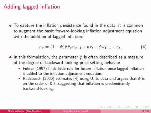
To capture the inflation persistence found in the data, it is commonto augment the basic forward-looking inflation adjustment equationwith the addition of lagged inflation:
πt = (1− φ)βEtπt+1 + κxt + φπt−1 + εt . (4)
In this formulation, the parameter φ is often described as a measureof the degree of backward-looking price setting behavior.
I Fuhrer (1997) finds little role for future inflation once lagged inflationis added to the inflation adjustment equation.
I Rudebusch (2000) estimates (4) using U. S. data and argues that φ ison the order of 0.7, suggesting that inflation is predominantlybackward-looking.
Noah Williams (UW Madison) New Keynesian model 17 / 52
Indexation
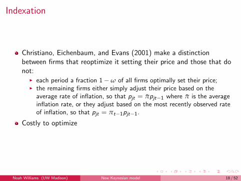
Christiano, Eichenbaum, and Evans (2001) make a distinctionbetween firms that reoptimize it setting their price and those that donot:
I each period a fraction 1−ω of all firms optimally set their price;I the remaining firms either simply adjust their price based on the
average rate of inflation, so that pjt = πpjt−1 where π is the averageinflation rate, or they adjust based on the most recently observed rateof inflation, so that pjt = πt−1pjt−1.
Costly to optimize
Noah Williams (UW Madison) New Keynesian model 18 / 52
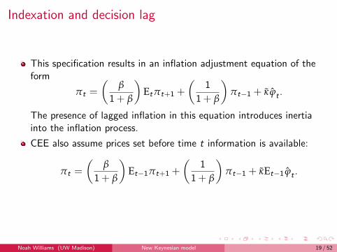
Indexation and decision lag
This specification results in an inflation adjustment equation of theform
πt =
(β
1 + β
)Etπt+1 +
(1
1 + β
)πt−1 + κ ϕt .
The presence of lagged inflation in this equation introduces inertiainto the inflation process.
CEE also assume prices set before time t information is available:
πt =
(β
1 + β
)Et−1πt+1 +
(1
1 + β
)πt−1 + κEt−1 ϕt .
Noah Williams (UW Madison) New Keynesian model 19 / 52
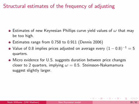
Structural estimates of the frequency of adjusting
Estimates of new Keynesian Phillips curve yield values of ω that maybe too high.
Estimates range from 0.758 to 0.911 (Dennis 2006)
Value of 0.8 implies prices adjusted on average every (1− 0.8)−1 = 5quarters.
Micro evidence for U.S. suggests duration between price changescloser to 2 quarters, implying ω = 0.5. Steinsson-Nakamamurasuggest slightly larger.
Noah Williams (UW Madison) New Keynesian model 20 / 52
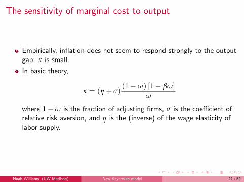
The sensitivity of marginal cost to output
Empirically, inflation does not seem to respond strongly to the outputgap: κ is small.
In basic theory,
κ = (η + σ)(1−ω) [1− βω]
ω
where 1−ω is the fraction of adjusting firms, σ is the coefficient ofrelative risk aversion, and η is the (inverse) of the wage elasticity oflabor supply.
Noah Williams (UW Madison) New Keynesian model 21 / 52

The sensitivity of marginal cost to output
So κ small if
ω large – high degree of price rigidity (estimates often implyunrealistic values around 0.8)
σ small – very little risk aversion
η is small – high degree of labor supply elasticity.
Noah Williams (UW Madison) New Keynesian model 22 / 52
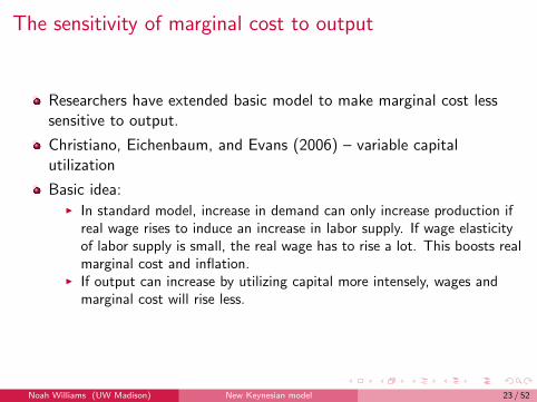
The sensitivity of marginal cost to output
Researchers have extended basic model to make marginal cost lesssensitive to output.
Christiano, Eichenbaum, and Evans (2006) – variable capitalutilization
Basic idea:I In standard model, increase in demand can only increase production if
real wage rises to induce an increase in labor supply. If wage elasticityof labor supply is small, the real wage has to rise a lot. This boosts realmarginal cost and inflation.
I If output can increase by utilizing capital more intensely, wages andmarginal cost will rise less.
Noah Williams (UW Madison) New Keynesian model 23 / 52
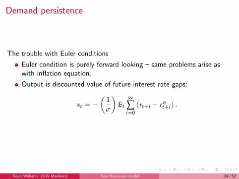
Demand persistence
The trouble with Euler conditions
Euler condition is purely forward looking – same problems arise aswith inflation equation.
Output is discounted value of future interest rate gaps:
xt = −(
1
σ
)Et
∞
∑i=0
(rt+i − rnt+i ) .
Noah Williams (UW Madison) New Keynesian model 24 / 52

Habit persistence
To match the hump shaped response of output seen in the data, habitpersistence has become a standard component of new Keynesianmodels (Christiano, Eichenbaum, and Evans 2006).
External Habit persistence: Marginal utility of current consumptiondepends on past aggregate consumption.
Internal Habit Persistence: Marginal utility of current consumptiondepends on household’s past consumption.
Noah Williams (UW Madison) New Keynesian model 25 / 52

General equilibrium, estimated models
Christiano, Eichenbaum, and Evans (2005)
Smets and Wouters (2003, 2007)
Levin, Onatski, Williams, and Williams (2006)I Components:
F Habit persistenceF Variable capital utilizationF Investment with 2nd-order adjustment costsF Price adjustment at start of period (based on expectations –
information delay)F Wage and price stickiness
Noah Williams (UW Madison) New Keynesian model 26 / 52

Conclusions
Basic model fairs poorly when faced with data – too forward-looking;
Habit persistence, variable capital utilization, firm specific capital,sticky wages all help.
Models fit data, but decomposition into flexible-price and gap maymiss major historical episodes.
Noah Williams (UW Madison) New Keynesian model 27 / 52

Policy analysis
Key issues
What are the objectives of optimal policy
Is the policy environment one of commitment or discretion?
What instrument rule implements the optimal policy?
What are the properties of the resulting equilibrium?
Noah Williams (UW Madison) New Keynesian model 28 / 52

Welfare
Given the specification of the economic environment, what are theappropriate objectives of the central bank?
Standard to assume central bank is concerned with minimizing aquadratic loss function that depended on output and inflation –plausible, but ultimately ad hoc. Common in the Barro-Gordontradition
Woodford (2003) has provided the most detailed analysis of the linkbetween a welfare criteria derived as a log-linear approximation to theutility of the representative agent and the type of quadratic lossfunctions so common in the literature.
Noah Williams (UW Madison) New Keynesian model 29 / 52
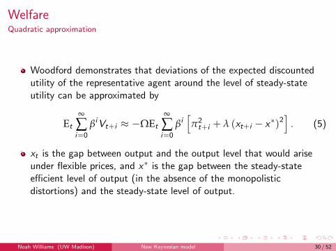
WelfareQuadratic approximation
Woodford demonstrates that deviations of the expected discountedutility of the representative agent around the level of steady-stateutility can be approximated by
Et
∞
∑i=0
βiVt+i ≈ −ΩEt
∞
∑i=0
βi[π2t+i + λ (xt+i − x∗)2
]. (5)
xt is the gap between output and the output level that would ariseunder flexible prices, and x∗ is the gap between the steady-stateefficient level of output (in the absence of the monopolisticdistortions) and the steady-state level of output.
Noah Williams (UW Madison) New Keynesian model 30 / 52
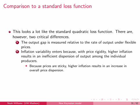
Comparison to a standard loss function
This looks a lot like the standard quadratic loss function. There are,however, two critical differences.
1 The output gap is measured relative to the rate of output under flexibleprices.
2 Inflation variability enters because, with price rigidity, higher inflationresults in an inefficient dispersion of output among the individualproducers.
F Because prices are sticky, higher inflation results in an increase inoverall price dispersion.
Noah Williams (UW Madison) New Keynesian model 31 / 52
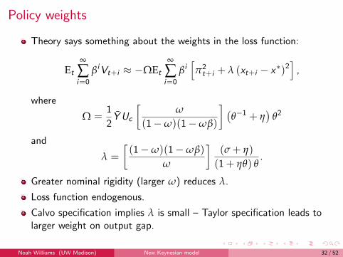
Policy weights
Theory says something about the weights in the loss function:
Et
∞
∑i=0
βiVt+i ≈ −ΩEt
∞
∑i=0
βi[π2t+i + λ (xt+i − x∗)2
],
where
Ω =1
2Y Uc
[ω
(1−ω)(1−ωβ)
] (θ−1 + η
)θ2
and
λ =
[(1−ω)(1−ωβ)
ω
](σ + η)
(1 + ηθ) θ.
Greater nominal rigidity (larger ω) reduces λ.
Loss function endogenous.
Calvo specification implies λ is small – Taylor specification leads tolarger weight on output gap.
Noah Williams (UW Madison) New Keynesian model 32 / 52
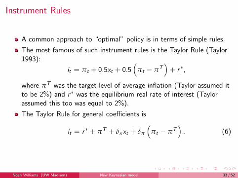
Instrument Rules
A common approach to “optimal” policy is in terms of simple rules.
The most famous of such instrument rules is the Taylor Rule (Taylor1993):
it = πt + 0.5xt + 0.5(
πt − πT)+ r ∗,
where πT was the target level of average inflation (Taylor assumed itto be 2%) and r ∗ was the equilibrium real rate of interest (Taylorassumed this too was equal to 2%).
The Taylor Rule for general coefficients is
it = r ∗ + πT + δxxt + δπ
(πt − πT
). (6)
Noah Williams (UW Madison) New Keynesian model 33 / 52
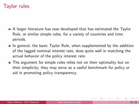
Taylor rules
A larger literature has now developed that has estimated the TaylorRule, or similar simple rules, for a variety of countries and timeperiods.
In general, the basic Taylor Rule, when supplemented by the additionof the lagged nominal interest rate, does quite well in matching theactual behavior of the policy interest rate.
The argument for simple rules relies not on their optimality but ontheir simplicity; they may serve as a useful benchmark for policy oraid in promoting policy transparency.
Noah Williams (UW Madison) New Keynesian model 34 / 52
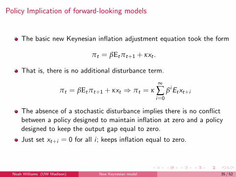
Policy Implication of forward-looking models
The basic new Keynesian inflation adjustment equation took the form
πt = βEtπt+1 + κxt .
That is, there is no additional disturbance term.
πt = βEtπt+1 + κxt ⇒ πt = κ∞
∑i=0
βiEtxt+i
The absence of a stochastic disturbance implies there is no conflictbetween a policy designed to maintain inflation at zero and a policydesigned to keep the output gap equal to zero.
Just set xt+i = 0 for all i ; keeps inflation equal to zero.
Noah Williams (UW Madison) New Keynesian model 35 / 52

Optimal policy in forward-looking models
Thus, the key implication of the basic new Keynesian model is thatprice stability is the appropriate objective of monetary policy.
No policy conflicts.
When prices are sticky but wages are flexible, the nominal wage canadjust to ensure labor market equilibrium is maintained in the face ofproductivity shocks. Optimal policy should then aim to keep the pricelevel stable.
Noah Williams (UW Madison) New Keynesian model 36 / 52

Policy implications of price stickiness
Models that combine optimizing agents and sticky prices have verystrong policy implications.
When the price level fluctuates, and not all firms are able to adjust,price dispersion results. This causes the relative prices of the differentgoods to vary. If the price level rises, for example, two things happen.
1 The relative price of firms who have not set their prices for a whilefalls. They experience in increase in demand and raise output, whilefirms who have just reset their prices reduce output. This productiondispersion is inefficient.
2 Consumers increase their consumption of the goods whose relativeprice has fallen and reduce consumption of those goods whose relativeprice has risen. This dispersion in consumption reduces welfare.
Noah Williams (UW Madison) New Keynesian model 37 / 52
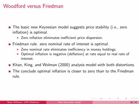
Woodford versus Friedman
The basic new Keynesian model suggests price stability (i.e., zeroinflation) is optimal.
I Zero inflation eliminates inefficient price dispersion.
Friedman rule: zero nominal rate of interest is optimal.I Zero nominal rate eliminates inefficiency in money holdings.I Optimal inflation is negative (deflation) at rate equal to real rate of
interest.
Khan, King, and Wolman (2000) analysis model with both distortions.
The conclude optimal inflation is closer to zero than to the Friedmanrule.
Noah Williams (UW Madison) New Keynesian model 38 / 52
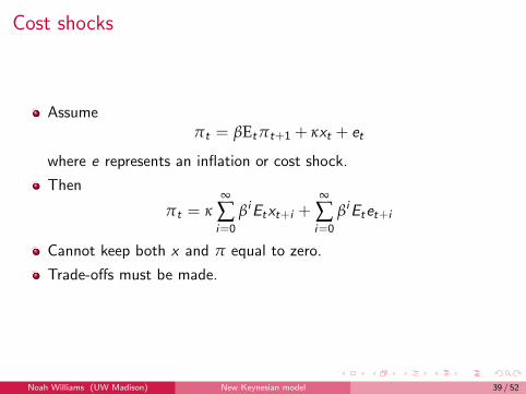
Cost shocks
Assumeπt = βEtπt+1 + κxt + et
where e represents an inflation or cost shock.
Then
πt = κ∞
∑i=0
βiEtxt+i +∞
∑i=0
βiEtet+i
Cannot keep both x and π equal to zero.
Trade-offs must be made.
Noah Williams (UW Madison) New Keynesian model 39 / 52
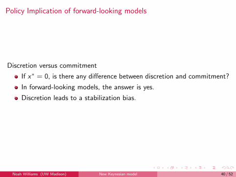
Policy Implication of forward-looking models
Discretion versus commitment
If x∗ = 0, is there any difference between discretion and commitment?
In forward-looking models, the answer is yes.
Discretion leads to a stabilization bias.
Noah Williams (UW Madison) New Keynesian model 40 / 52
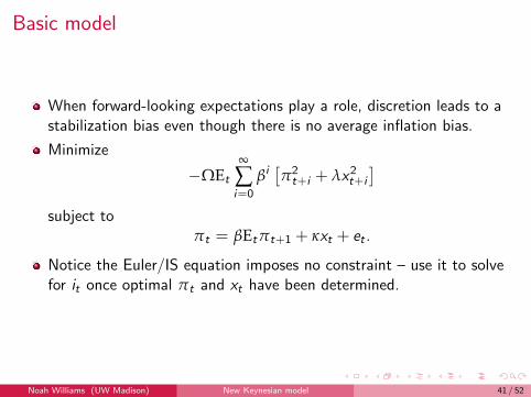
Basic model
When forward-looking expectations play a role, discretion leads to astabilization bias even though there is no average inflation bias.
Minimize
−ΩEt
∞
∑i=0
βi[π2t+i + λx2t+i
]subject to
πt = βEtπt+1 + κxt + et .
Notice the Euler/IS equation imposes no constraint – use it to solvefor it once optimal πt and xt have been determined.
Noah Williams (UW Madison) New Keynesian model 41 / 52
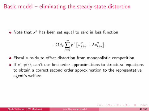
Basic model – eliminating the steady-state distortion
Note that x∗ has been set equal to zero in loss function
−ΩEt
∞
∑i=0
βi[π2t+i + λx2t+i
].
Fiscal subsidy to offset distortion from monopolistic competition.
If x∗ 6= 0, can’t use first order approximations to structural equationsto obtain a correct second order approximation to the representativeagent’s welfare.
Noah Williams (UW Madison) New Keynesian model 42 / 52
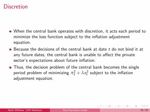
Discretion
When the central bank operates with discretion, it acts each period tominimize the loss function subject to the inflation adjustmentequation.
Because the decisions of the central bank at date t do not bind it atany future dates, the central bank is unable to affect the privatesector’s expectations about future inflation.
Thus, the decision problem of the central bank becomes the singleperiod problem of minimizing π2
t + λx2t subject to the inflationadjustment equation.
Noah Williams (UW Madison) New Keynesian model 43 / 52
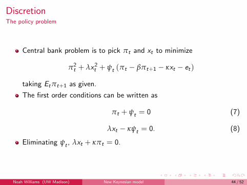
DiscretionThe policy problem
Central bank problem is to pick πt and xt to minimize
π2t + λx2t + ψt (πt − βπt+1 − κxt − et)
taking Etπt+1 as given.
The first order conditions can be written as
πt + ψt = 0 (7)
λxt − κψt = 0. (8)
Eliminating ψt , λxt + κπt = 0.
Noah Williams (UW Madison) New Keynesian model 44 / 52
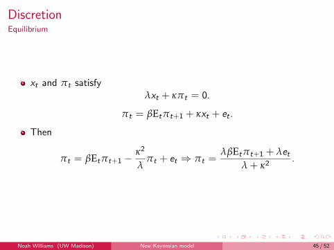
DiscretionEquilibrium
xt and πt satisfyλxt + κπt = 0.
πt = βEtπt+1 + κxt + et .
Then
πt = βEtπt+1 −κ2
λπt + et ⇒ πt =
λβEtπt+1 + λetλ + κ2
.
Noah Williams (UW Madison) New Keynesian model 45 / 52
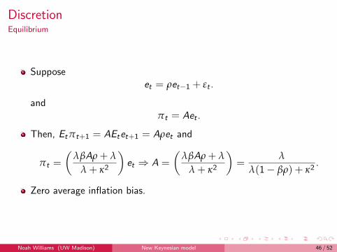
DiscretionEquilibrium
Supposeet = ρet−1 + εt .
andπt = Aet .
Then, Etπt+1 = AEtet+1 = Aρet and
πt =
(λβAρ + λ
λ + κ2
)et ⇒ A =
(λβAρ + λ
λ + κ2
)=
λ
λ(1− βρ) + κ2.
Zero average inflation bias.
Noah Williams (UW Madison) New Keynesian model 46 / 52
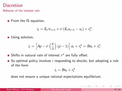
DiscretionBehavior of the interest rate
From the IS equation,
it = Etπt+1 + σ (Etxt+1 − xt) + rnt .
Using solution,
it =[Aρ− σ
( κ
λ
)(ρ− 1)
]et + rnt = Bet + rnt .
Shifts in natural rate of interest rn are fully offset.
So optimal policy involves i responding to shocks, but adopting a ruleof the form
it = Bet + rnt
does not ensure a unique rational expectations equilibrium.
Noah Williams (UW Madison) New Keynesian model 47 / 52
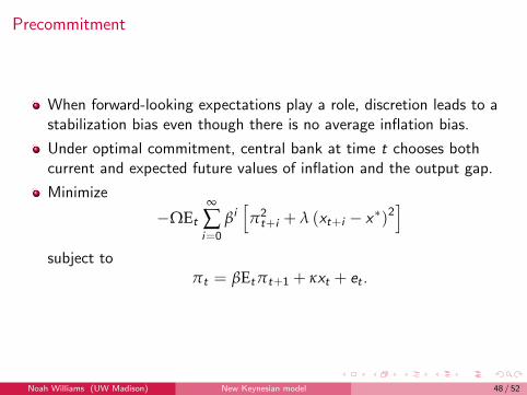
Precommitment
When forward-looking expectations play a role, discretion leads to astabilization bias even though there is no average inflation bias.
Under optimal commitment, central bank at time t chooses bothcurrent and expected future values of inflation and the output gap.
Minimize
−ΩEt
∞
∑i=0
βi[π2t+i + λ (xt+i − x∗)2
]subject to
πt = βEtπt+1 + κxt + et .
Noah Williams (UW Madison) New Keynesian model 48 / 52
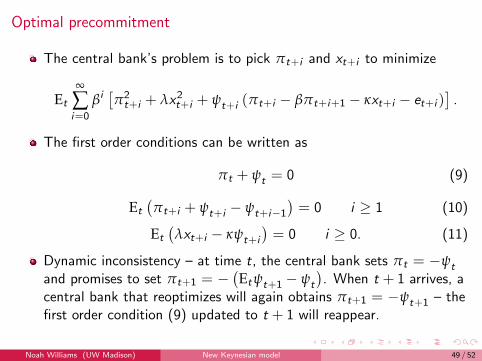
Optimal precommitment
The central bank’s problem is to pick πt+i and xt+i to minimize
Et
∞
∑i=0
βi[π2t+i + λx2t+i + ψt+i (πt+i − βπt+i+1 − κxt+i − et+i )
].
The first order conditions can be written as
πt + ψt = 0 (9)
Et
(πt+i + ψt+i − ψt+i−1
)= 0 i ≥ 1 (10)
Et
(λxt+i − κψt+i
)= 0 i ≥ 0. (11)
Dynamic inconsistency – at time t, the central bank sets πt = −ψt
and promises to set πt+1 = −(Etψt+1 − ψt
). When t + 1 arrives, a
central bank that reoptimizes will again obtains πt+1 = −ψt+1 – thefirst order condition (9) updated to t + 1 will reappear.
Noah Williams (UW Madison) New Keynesian model 49 / 52
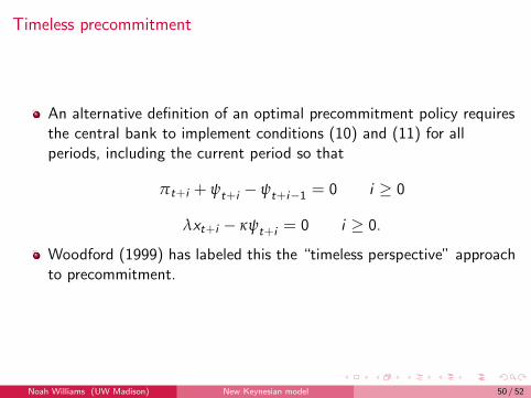
Timeless precommitment
An alternative definition of an optimal precommitment policy requiresthe central bank to implement conditions (10) and (11) for allperiods, including the current period so that
πt+i + ψt+i − ψt+i−1 = 0 i ≥ 0
λxt+i − κψt+i = 0 i ≥ 0.
Woodford (1999) has labeled this the “timeless perspective” approachto precommitment.
Noah Williams (UW Madison) New Keynesian model 50 / 52
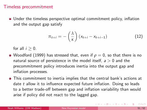
Timeless precommitment
Under the timeless perspective optimal commitment policy, inflationand the output gap satisfy
πt+i = −(
λ
κ
)(xt+i − xt+i−1) (12)
for all i ≥ 0.
Woodford (1999) has stressed that, even if ρ = 0, so that there is nonatural source of persistence in the model itself, a > 0 and theprecommitment policy introduces inertia into the output gap andinflation processes.
This commitment to inertia implies that the central bank’s actions atdate t allow it to influence expected future inflation. Doing so leadsto a better trade-off between gap and inflation variability than wouldarise if policy did not react to the lagged gap.
Noah Williams (UW Madison) New Keynesian model 51 / 52
Improved trade-off under commitment
The difference in the stabilization response under commitment anddiscretion is the stabilization bias due to discretion.
Consider a positive inflation shock, e > 0.
A given change in current inflation can be achieved with a smaller fallin x if expected future inflation can be reduced:
πt = βEtπt+1 + κxt + et
Requires a commitment to future deflation.
By keeping output below potential (a negative output gap) for severalperiods into the future after a positive cost shock, the central bank isable to lower expectations of future inflation. A fall in Etπt+1 at thetime of the positive inflation shock improves the trade-off betweeninflation and output gap stabilization faced by the central bank.
Noah Williams (UW Madison) New Keynesian model 52 / 52