Midterm 1 Practice Solutions - DSpace@MIT: Home · Midterm 1 Practice Solutions — Spring 09 5 4...

Midterm 1 Practice Solutions

1 Robot behavior

1.

class TBTurnSmoothly(SM): def getNextValues(self, state, inp):

currentTheta = inp.odometry.thetareturn (state,

io.Action(rvel = self.rotationalGain * (thetaDesired currentTheta),

fvel = 0))

2. The difference equations are:

Θ[n] = Θ[n − 1] + TΩ[n − 1]

Ω[n] = K(Θdes[n − 1] − Θ[n − 1])

The operator version is:

(1 − R)Θ = TRΩ

Ω = KR(Θdes − Θ)

Combining we get:

1 − RΘ + KTR2Θ = KTR2Θdes

We accepted a number of variations.

3. The system function is:

Θ KTR2

= Θdes 1 − RΘ + KTR2

Substitute R = 1/z in the denominator polynomial and we get:

z 2 − z + KT

The roots of this polynomial are the poles:

1±√

1 − 4KT

2

Note that for K = 0, one of the poles is 1.0. For K < 0, one of the poles is always greater than 1.0. This makes sense since for K < 0, the feedback increases the error.

Midterm 1 Practice Solutions — Spring 09 2

For T = 0.2, for K = 5, we have a pole of magnitude 1.0 and they get bigger with bigger gain. The range of stable K is 0 < K < 5

In general, when 4KT > 1 we have complex poles. For monotonic convergence we need real poles, so we want:

0 < K <= 1/(4T)

Note that when K = 1/(4T), we have the lowest magnitude pole, the pole approaches 1 as K

decreases towards 0, so:

For T = 0.2, the best value of K is 1.25, which leads to a pole of 1/2.

4. The analysis above shows that when T increases the range of stable gains decreases. Basically the effective gain is KT . As the T increases we need smaller and smaller gains to keep monotonic convergence. The result is very sluggish performance.

5.

Θ[n] = Θ[n − 1] + TΩ[n − 1]

Ω[n] = Ω[n − 1] + TΞ[n − 1]

Ξ[n] = K1E[n] + K2E[n − 1]

E[n] = Θdes[n] − Θ[n]

where Ξ is the acceleration. So, basically, the velocity is the integrated acceleration and the position is the integrated velocity. And, the acceleration is given by the gains times the position errors.

def robot(k1, k2):dt = 0.2control = sf.SystemFunction(poly.Polynomial([k2, k1]),

poly.Polynomial([1]))vel = sf.SystemFunction(poly.Polynomial([T, 0]),

poly.Polynomial([-1, 1]))pos = sf.SystemFunction(poly.Polynomial([T, 0]),

poly.Polynomial([-1, 1]))rob = sf.FeedbackSubtract(sf.Cascade(control,

sf.Cascade(vel, pos)))return abs(rob.dominantPole())

Depending on the resolution of the search, one gets very different answers.

optOverGrid(robot, -10, 10, -10, 10, 1, 1)(0.99999999999999956, (1, -1))optOverGrid(robot, -10, 10, -10, 10, 0.5, 0.5)(0.84617988641100905, (2.5, -2.0))optOverGrid(robot, -10, 10, -10, 10, 0.25, 0.25)(0.74999999999999933, (1.75, -1.5))optOverGrid(robot, -10, 10, -10, 10, 0.1, 0.1)(0.68863445766586584, (1.4999999999999816, -1.3000000000000189))


2 Weighted Objective

1.

There are many ways of writing this. Here are a few.

def argmax(elements, f):bestScore = NonebestElement = Nonefor e in elements:

score = f(e) if bestScore == None or score > bestScore:

bestScore = scorebestElement = e

return bestElement

def argmax(elements, f):bestElement = elements[0]for e in elements:

if f(e) > f(bestElement):bestElement = e

return bestElement

def argmax(elements, f):vals = [f(e) for e in elements]return elements[vals.index(max(vals))]

def argmax(elements, f):return max(elements, key=f])

2.

Here are a couple that work:

WOPQ([Fish.length, Fish.width], [0.9, 0.1])WOPQ([lambda x: x.length(), lambda x: x.width()], [0.9, 0.1])

3.

def extract(self):def priority(e):

return sum([w*f(e) for (w,f) in zip(self.weights,self.features)]) best = argmax(self.elements, priority) self.elements.remove(best) return best

4.

wopq.extract() = Sydney

Sydney is the longest fish and the priority weights heavily favor length.


5.

class WOPQ(FPQ):def __init__(self, features, weights):

def priority(e):return sum([w*f(e) for (w,f) in zip(weights,features)])

FPQ.__init__(self, priority)

That’s it... the other methods are provided by the FPQ class.

6.

def featureRange(feature, elements):vals = [feature(e) for e in elements]return max(vals) - min(vals)

def selectFeatures(features, n, elements):return sorted(features, key = featureRange)[-n : ]

3 More Oop You are told that we have a class A, with one initialization argument, with a method f that takes one argument and returns a number.

>>> x = A(2)>>> x.f(3)9

Define a class B that is a subclass of class A. Class B has the same initialization as A and a method f that returns twice whatever value the f method of A would return. You don’t need to know what the code for A is.

>>> x = B(2)>>> x.f(3)18

class B(A):def f(self, x):

return A.f(self, x)*2

2 points for correct answer (no __init__, passing self)1 point for minor error


4 In the Tank Imagine a cylindrical water tank with a source of water entering the bottom of the tank and a sensor to measure the depth of the water. The source of water can be adjusted so that water enters (or exits) the tank at a desired rate. In addition to this controlled source of water, there is also a leak in the tank, through which water flows regardless of the controlled flow. The diameter of the tank is such that one inch in depth is one gallon of water. The following variables characterize this problem:

• d[t] is the depth, in inches, of the water in the tank at time t.

• v[t] is the volume of water that flows through the controlled source of water in the time interval [t, t + 1].

• o[t] is the volume of water that leaks from the tank in the time interval [t, t + 1]. Assume o[t]

is proportional to d[t], with a proportionality constant of 0.1

• g[t] is the desired (goal) depth of water (in inches) in the tank at time t

• s[t] is the sensed depth (in inches) of water in the tank at time t; assume the sensor introduces one unit of delay, so that s[t] = d[t − 1]

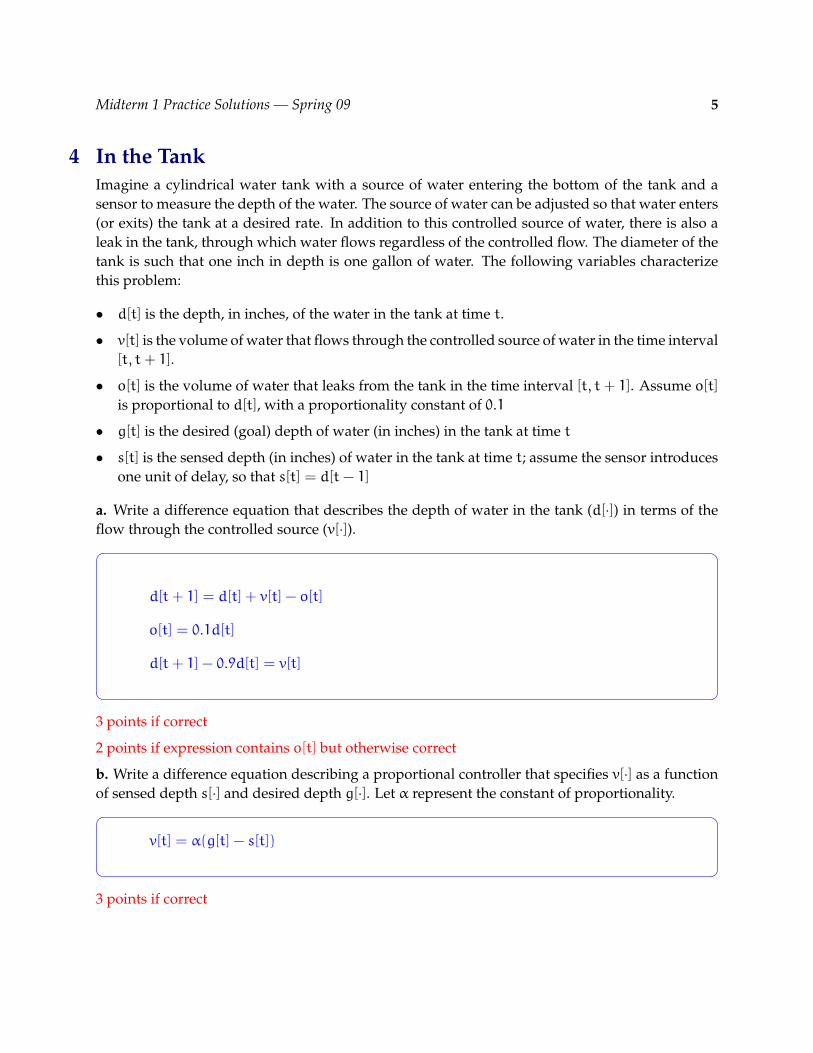
a. Write a difference equation that describes the depth of water in the tank (d[ ]) in terms of the ·flow through the controlled source (v[ ]).·

d[t + 1] = d[t] + v[t] − o[t]

o[t] = 0.1d[t]

d[t + 1] − 0.9d[t] = v[t]

3 points if correct

2 points if expression contains o[t] but otherwise correct

b. Write a difference equation describing a proportional controller that specifies v[ ] as a function ·of sensed depth s[ ] and desired depth g[ ]. Let α represent the constant of proportionality. · ·

v[t] = α(g[t] − s[t])

3 points if correct


5 Linear Systems (20 points) Part a. Several systems are illustrated below. The left column shows block diagrams. The right column shows system functions and pole locations for k = 0.9. Indicate which panel on the right (if any) corresponds to each panel on the left by drawing a straight line from A, B, C, and/or D to its partner. [Your answer should include 4 or fewer straight lines.]

R R R+ + +

k

k

k

X Y− − −

A

Y

X= R3

kR3 + kR2 + kR+ 1

poles: 1.72; −0.41± 0.59j

E

R R R+

k

X Y−

B

Y

X= 1

kR3 + 1

poles: −0.48± 0.84j; 0.96

F

R R R+ + +

k k k

X Y− − −

C

Y

X= R3

kR3 + 1

poles: −0.48± 0.84j; 0.96

G

R R

R

+

k

X Y−

D

Y

X= R3

k3R3 + 3k2R2 + 3kR+ 1

poles: 0.9; 0.9; 0.9

H

A E +3 points if correct → →

B G +3 points if correct → →

C H +3 points if correct → →

D nowhere +2 points if correct → →


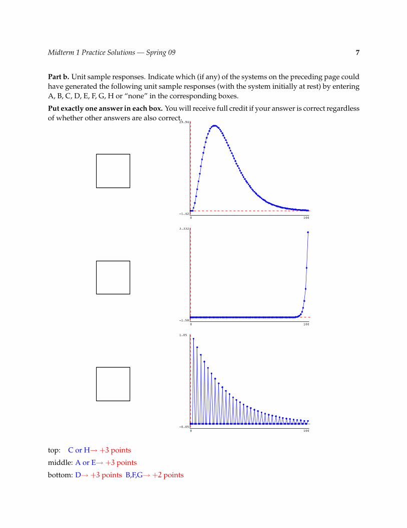
Part b. Unit sample responses. Indicate which (if any) of the systems on the preceding page could have generated the following unit sample responses (with the system initially at rest) by entering A, B, C, D, E, F, G, H or “none” in the corresponding boxes.

Put exactly one answer in each box. You will receive full credit if your answer is correct regardless of whether other answers are also correct.

29.94

-1.420 100

3.332

-1.580 100

1.05

-0.050 100

top: C or H +3 points→

middle: A or E +3 points→

bottom: D +3 points B,F,G +2 points→ →


6 Python and OOP (20 points) Part a. What does this program print? Write your answers in the boxes provided.

class NN:def __init__(self):

self.n = 0def get(self):

self.n += 1return str(self.n)

def reset(self):self.n = 0

class NS(NN):def get(self, s):

return s + NN.get(self)foo = NS()print foo.get(’a’)

a1

print foo.get(’b’)

b2

foo.reset()print foo.get(’c’)

c1


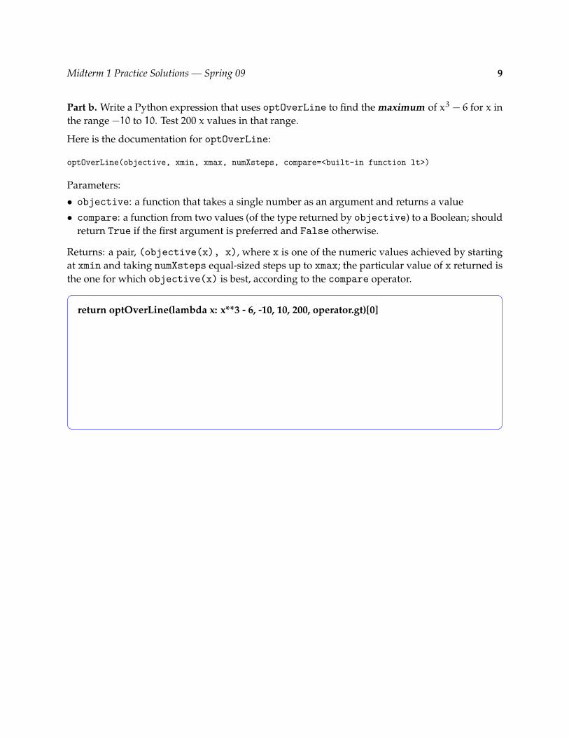
Part b. Write a Python expression that uses optOverLine to find the maximum of x3 − 6 for x in the range −10 to 10. Test 200 x values in that range.

Here is the documentation for optOverLine:

optOverLine(objective, xmin, xmax, numXsteps, compare=<built-in function lt>)

Parameters:

objective: a function that takes a single number as an argument and returns a value •

compare: a function from two values (of the type returned by objective) to a Boolean; should • return True if the first argument is preferred and False otherwise.

Returns: a pair, (objective(x), x), where x is one of the numeric values achieved by starting at xmin and taking numXsteps equal-sized steps up to xmax; the particular value of x returned is the one for which objective(x) is best, according to the compare operator.

return optOverLine(lambda x: x**3 - 6, -10, 10, 200, operator.gt)[0]


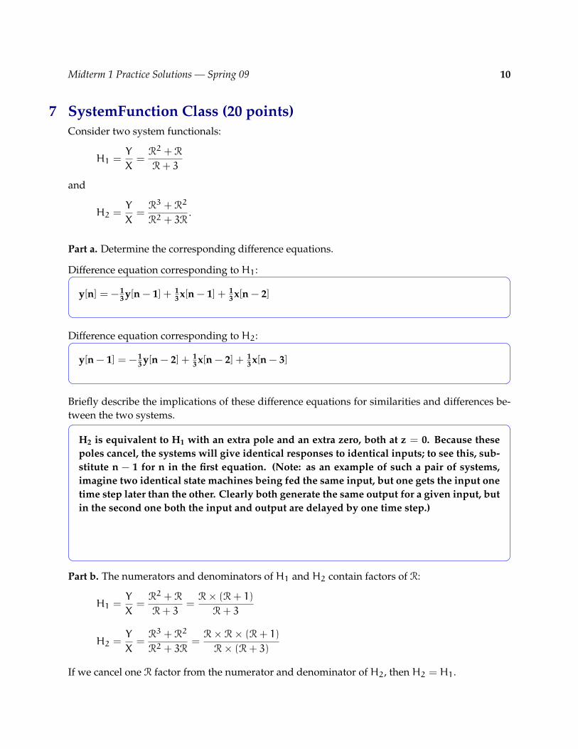
7 SystemFunction Class (20 points) Consider two system functionals:

Y R2 + R H1 = =

X R + 3

and

Y R3 + R2

H2 = = . X R2 + 3R

Part a. Determine the corresponding difference equations.

Difference equation corresponding to H1:

y[n] = −1 3 y[n − 1] + 1

3 x[n − 1] + 1 3 x[n − 2]

Difference equation corresponding to H2:

y[n − 1] = −1 3 y[n − 2] + 1

3 x[n − 2] + 1 3 x[n − 3]

Briefly describe the implications of these difference equations for similarities and differences between the two systems.

H2 is equivalent to H1 with an extra pole and an extra zero, both at z = 0. Because these poles cancel, the systems will give identical responses to identical inputs; to see this, substitute n − 1 for n in the first equation. (Note: as an example of such a pair of systems, imagine two identical state machines being fed the same input, but one gets the input one time step later than the other. Clearly both generate the same output for a given input, but in the second one both the input and output are delayed by one time step.)

Part b. The numerators and denominators of H1 and H2 contain factors of R:

Y R2 + R R× (R + 1)H1 = = =

X R + 3 R + 3

Y R3 + R2 R× R× (R + 1)H2 = = =

X R2 + 3R R× (R + 3)

If we cancel one R factor from the numerator and denominator of H2, then H2 = H1.


Write a Python function called ReducedSystemFunction, which

takes an input inp of type SystemFunction,•

cancels all factors of R that are common to the numerator and denominator of inp, and •

returns the result as a new object of type SystemFunction.•

ReducedSystemFunction should not modify inp. Some relevant software documentation follows the box. You can assume that we have already import sf and poly.

def ReducedSystemFunction(inp): num= inp.numerator.coeffs[:] den= inp.denominator.coeffs[:] while num[-1] == 0 and den[-1] == 0:

num.pop() den.pop()

return sf.SystemFunction(poly.Polynomial(num), poly.Polynomial(den))

Attributes of SystemFunction Class:

__init__(self, numPoly, denomPoly) poles(self) returns a list of the poles of the system poleMagnitudes(self) returns a list of the magnitudes of the poles of the system dominantPole(self) returns the pole with the largest magnitude __add__(self, other) numerator Polynomial in R representing the numerator denominator Polynomial in R representing the denominator

Attributes of Polynomial Class:

__init__(self, coeffs) add(p1, p2) returns a new polynomial, which is sum __add__(p1, p2) __sub__(p1, p2) scalarMult(self, s) returns a new polynomial, with coefs multiplied by s mul(p1, p2) returns a new polynomial equal to the product __mul__(p1, p2) val(self, x) returns value of polynomial with variable assigned to x roots(self) return list of roots coeffs list of polynomial coefficients, highest order first order polynomial order; one less than number of coeffs


8 Inheritance and State Machines (20 points) Recall that we have defined a Python class sm.SM to represent state machines. Here we consider a special type of state machine, whose states are always integers that start at 0 and increment by 1 on each transition. We can represent this new type of state machines as a Python subclass of sm.SM called CountingStateMachine.

We wish to use the CountingStateMachine class to define new subclasses that each provide a single new method getOutput(self, state, inp) which returns just the output for that state and input; the CountingStateMachine will take care of managing and incrementing the state, so its subclasses don’t have to worry about it.

Here is an example of a subclass of CountingStateMachine.

class CountMod5(CountingStateMachine):def getOutput(self, state, inp):

return state % 5

Instances of CountMod5 generate output sequences of the form 0, 1, 2, 3, 4, 0, 1, 2, 3, 4, 0, . . ..

Part a. Define the CountingStateMachine class. Since CountingStateMachine is a subclass of sm.SM, you will have to provide definitions of the startState instance variable and get-NextValues method, just as we have done for other state machines. You can assume that every subclass of CountingStateMachine will provide an appropriate getOutput method.

class CountingStateMachine(sm.SM): def __init__(self):

self.startState= 0 def getNextState(self, state, inp):

return(state + 1, self.getOutput(state, inp))


Part b. Define a subclass of CountingStateMachine called AlternateZeros. Instances of AlternateZeros should be state machines for which, on even steps, the output is the same as the input, and on odd steps, the output is 0. That is, given inputs, i0, i1, i2, i3, . . ., they generate outputs, i0, 0, i2, 0, . . ..

class AlternateZeros(CountingStateMachine): def getOutput(self, state, inp):

if not state % 2: return inp

return 0


9 Signals and Systems (20 points) Let H represent a system whose input is a signal X and whose output is a signal Y. The system H

is defined by the following difference equations:

y[n] = x[n] + z[n]

z[n] = y[n − 1] + z[n − 1]

Part a. Which of the following systems are valid representations of H? (Remember that there can be multiple “equivalent” representations for a system.)

+ +

R R2 −1

X Y

equivalent to H (yes/no)? YES

+ +

R R2 2

X Y

equivalent to H (yes/no)? NO

+

+

R

R

X Y

equivalent to H (yes/no)? YES

+ +

R

R

−1

X Y

equivalent to H (yes/no)? NO

Part b. Assume that the system starts “at rest” and that the input signal X is the unit sample signal. Determine y[3].

y[3] = 4

Part c. Let po represent the dominant pole of H. Determine po.

Enter p0 or none if there are no poles: 2


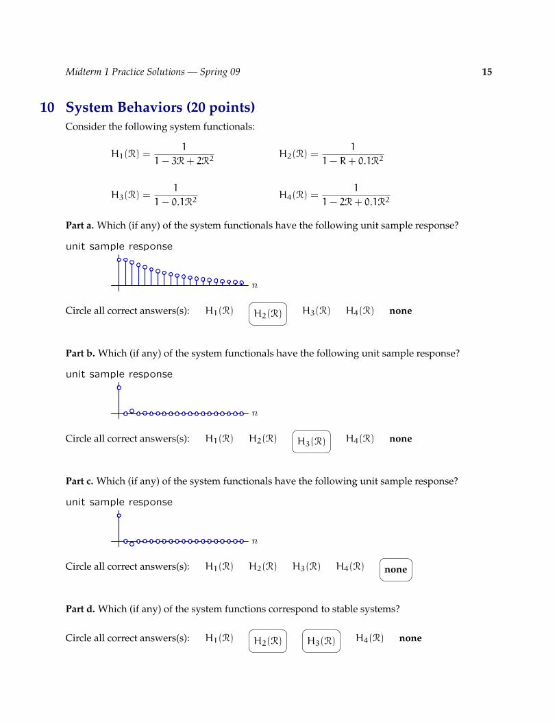
10 System Behaviors (20 points) Consider the following system functionals:

H1(R) = 1

1 − 3R + 2R2 H2(R) =

1

1 − R + 0.1R2

1 1 H3(R) = H4(R) =

1 − 0.1R2 1 − 2R + 0.1R2

Part a. Which (if any) of the system functionals have the following unit sample response?

n

unit sample response

Circle all correct answers(s): H1(R) H2(R) H3(R) H4(R) none

Part b. Which (if any) of the system functionals have the following unit sample response?

n



Part c. Which (if any) of the system functionals have the following unit sample response?

n



Part d. Which (if any) of the system functions correspond to stable systems?


MIT OpenCourseWarehttp://ocw.mit.edu

6.01 Introduction to Electrical Engineering and Computer Science IFall 2009

For information about citing these materials or our Terms of Use, visit: http://ocw.mit.edu/terms.

http://ocw.mit.edu

http://ocw.mit.edu/terms

Midterm 1 Practice Solutions - DSpace@MIT: Home · Midterm 1 Practice Solutions — Spring 09 5 4...

Documents

Transcript of Midterm 1 Practice Solutions - DSpace@MIT: Home · Midterm 1 Practice Solutions — Spring 09 5 4...