WORKING PAPER SERIES 1-2016

Πατησίων 76, 104 34 Αθήνα. Tηλ.: 210 8203303-5 / Fax: 210 8238249 76, Patission Street, Athens 104 34 Greece. Tel.: (+30) 210 8203303-5 / Fax: (+30) 210 8238249

E-mail: econ@aueb.gr / www.aueb.gr

Market and Political Power Interactions in Greece: A Theory

by

Tryphon Kollintzas, Dimitris Papageorgiou, and Vanghelis Vassilatos

Market and Political Power Interactions in Greece: A Theory

Tryphon Kollintzasa, Dimitris Papageorgioub, and Vanghelis Vassilatosc

February 2, 2016

Abstract: In recent years the growth pattern of Greece has been disturbed, as this country is suffering from a persisting economic crisis that goes beyond the usual business cycle. In this paper, we develop a neoclassical growth model of market and political power interactions that explains this crisis. The model incorporates the insiders-outsiders labor market structure and the concept of an elite government. Outsiders form a group of workers that supply labor to a competitive private sector. And, insiders form a group of workers that enjoy market power in supplying labor to the public sector and influence the policy decisions of government, including those that affect the development and maintenance of public sector infrastructures. This leads to labor misallocation and inefficient fiscal policies. Despite the fact that expanding public sector output has a positive effect on growth, eventually this is counterbalanced by the labor misallocation and inefficient tax policy outcomes. Thus, the deep and sustained growth reversal occurring in Greece is explained as a consequence of the organizational structure of the labor market, that has important implications on the workings of the economic and political systems. JEL classification: P16; O43; J45; O52 Keywords: Insiders - Outsiders; Politicoeconomic Equilibrium; Taxation; Fiscal Policy; Growth; Greek Crisis a Athens University of Economics and Business and CEPR (kollintzas@hol.gr) b Bank of Greece, Economic Analysis and Research Department (dpapag@aueb.gr) c Athens University of Economics and Business (vvassila@aueb.gr)

1“Too many politicians and economists blame austerity – urged by Greece’s creditors – for the collapse of the Greek economy. But the data show neither marked austerity by historical standards nor government cutbacks severe enough to explain the huge job losses. What the data do show are economic ills rooted in the values and beliefs of Greek society. Greece’s public sector is rife with clientelism (to gain votes) and cronyism (to gain favors) – far more so than in other parts of Europe”. Edmund S. Phelps, 2006 Nobel laureate in Economics*

*Project Syndicate, September 4, 2015. Link: http://www.project-syndicate.org/columnist/edmund-s--phelps.

21. INTRODUCTION

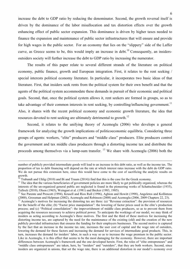
In recent years the growth pattern of Greece has been disturbed, as this country is suffering

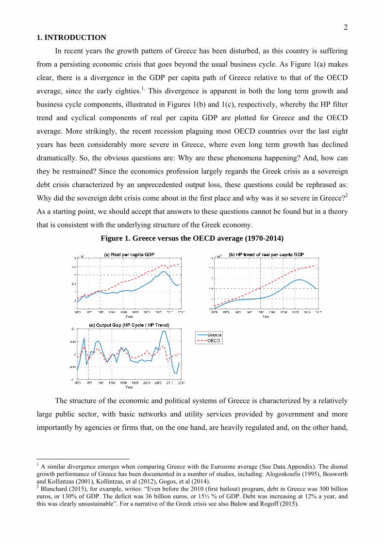
from a persisting economic crisis that goes beyond the usual business cycle. As Figure 1(a) makes

clear, there is a divergence in the GDP per capita path of Greece relative to that of the OECD

average, since the early eighties.1, This divergence is apparent in both the long term growth and

business cycle components, illustrated in Figures 1(b) and 1(c), respectively, whereby the HP filter

trend and cyclical components of real per capita GDP are plotted for Greece and the OECD

average. More strikingly, the recent recession plaguing most OECD countries over the last eight

years has been considerably more severe in Greece, where even long term growth has declined

dramatically. So, the obvious questions are: Why are these phenomena happening? And, how can

they be restrained? Since the economics profession largely regards the Greek crisis as a sovereign

debt crisis characterized by an unprecedented output loss, these questions could be rephrased as:

Why did the sovereign debt crisis come about in the first place and why was it so severe in Greece?2

As a starting point, we should accept that answers to these questions cannot be found but in a theory

that is consistent with the underlying structure of the Greek economy.

Figure 1. Greece versus the OECD average (1970-2014)

The structure of the economic and political systems of Greece is characterized by a relatively

large public sector, with basic networks and utility services provided by government and more

importantly by agencies or firms that, on the one hand, are heavily regulated and, on the other hand,

1 A similar divergence emerges when comparing Greece with the Eurozone average (See Data Appendix). The dismal growth performance of Greece has been documented in a number of studies, including: Alogoskoufis (1995), Bosworth and Kollintzas (2001), Kollintzas, et al (2012), Gogos, et al (2014). 2 Blanchard (2015), for example, writes: “Even before the 2010 (first bailout) program, debt in Greece was 300 billion euros, or 130% of GDP. The deficit was 36 billion euros, or 15½ % of GDP. Debt was increasing at 12% a year, and this was clearly unsustainable”. For a narrative of the Greek crisis see also Bulow and Rogoff (2015).

3labor therein is organized in powerful independent unions.3,4 Moreover, there are important strategic

interactions between these unions and the government that create a bias for high spending and

consequently for high taxes and high debt accumulation.5

In this paper, we develop a dynamic general equilibrium model of market and political power

interactions, based on a synthesis of the insiders-outsiders labor market structure of Lindbeck and

Snower (1986) and the concept of an elite government of Acemoglu (2006), as this elite coincides

with the group of insiders. That is, we identify insiders as a group of workers that enjoy market

power in supplying labor to the public sector and influence the policy decisions of government,

including those that affect public finances through the development and maintenance of public

sector infrastructures. And, we identify outsiders as a group of workers that supply labor to a

competitive private sector. Thus, wages differ across identical labor services due to the particular

organization of the labor market.6 Although insiders and outsiders are identical, the wages of

insiders are higher than those of the outsiders, creating, what we call the “labor misallocation

effect,” that lowers output and output growth towards the steady state.

More specifically, outsiders work on the production of a final good, while insiders work on

the production of intermediate goods, produced by monopolies controlled by government. For that

reason, intermediate goods enter the final goods production function through a Dixit-Stiglitz

aggregator that incorporates the so called “variety” effect, whereby an increase in the number of

intermediate goods increases output. Further, this aggregator allows for intermediate goods to be

gross complements, as one should think of the services of various network infrastructures, provided

by the State (e.g., power, water, phone, roads, railways, harbors, airports, etc.). Thus, by

construction, public sector involvement is prima facie beneficial for growth. Nevertheless, and in

anticipation of the results of the model, this feature does not prevent public sector expansion being

detrimental to growth. 3 Total government spending as a share to GDP in the pre-crisis year 2007 in Greece was 46.93%. This is not much higher relative to the Eurozone 15 average of 45.33, but considerably than the OECD average of 39.01. However, it is not so much the size of the government that is in question, here, but the fact that the Greek state is widely taken to be one of the most interfering in the workings of the economy (See, e.g., the 2015 OECD study by Koske, et al.). 4 Chapter 1 of the “Industrial Relations in Europe 2012” extensive report of the European Commission (2013) places Greece along with other Southern European countries in the industrial relations system cluster, referred to as “state-centered.” And, in Chapter 3, the same cluster of countries is identified when it comes to public sector industrial relations. Similar classifications with respect to wage bargaining institutions have been made in Visser (2013) and European Commission (2014). 5 This interaction has been recognized in the political science literature since the late seventies (Schmitter (1977), Sargent (1985), Cawson (1986)) and recently has been explicitly pointed out for Greece by Featherstone (2008). 6 In the insiders-outsiders theory of Lindbeck and Snower (1986), some worker participants (“insiders”) have privileged positions relative to others (“outsiders”). Insiders get market power by resisting competition in a variety of ways, including harassing firms and outsiders that try to hire/be hired, by underbidding the wages of insiders and by influencing pertinent legislation (Saint-Paul (1996)). There has been no association of the wage premium in the public sector and insiders-outsiders labor market, to our knowledge, in the literature. However, the importance of insiders-outsiders labor markets for providing the microeconomic foundations for justifying the strength of unions has been at the core of this literature (see, e.g., the survey by Lindbeck and Snower (2001)). As already mentioned, in the previous footnote, the strength of the unions in the public sector in the South European countries has been noticed in the political science literature.

4The wage rate of outsiders is determined competitively. Each intermediate good producer

prices its output satisfying a zero profit condition, taking the wage rate offered by the corresponding

insiders’ union as given. This determines each intermediate good producer’s employment and

output. Then, the corresponding wage rate is determined by the respective union that takes the

demand for labor it faces, as given. This is the well known Monopoly-Union model of McDonald

and Solow (1981) and Oswald (1983). Since there are as many independent unions of insiders as

there are intermediate good producers, overall equilibrium in the market for insiders’ labor is

characterized by a Nash equilibrium among all insiders’ unions. This modeling choice is, again,

consistent with Greek labor market institutions, as well as those of other Southern European

countries, where the wage setting process in the public sector is characterized by trade union

fragmentation and, at the same time, lack of co-ordination.7 This is quite different from other

typically identified country clusters. For example, in Anglo-Saxon countries wage bargaining is

thought, in general, to be competitive and labor unions are thought to play a relatively small role in

wage setting. On the other hand, in the Nordic countries, labor unions in all sectors are thought to

be powerful but cooperative, thereby internalizing the externalities associated with a high wage

premium of one industry/sector on the rest.8

In the symmetric equilibrium case, given reasonable parameter restrictions, the ratio of the

wage rate of insiders over that of the outsiders (i.e., the public sector wage premium) is greater than

one and increasing in the degree intermediate goods are gross complements, as well as in the

number of publicly provided intermediate goods. Moreover, the wage premium and the ratio of

employment in the public sector over total employment are inversely related, giving rise to the

“labor misallocation effect”. For a fixed number of insiders’ unions, this model is formally

equivalent to a standard Cass-Koopmans neoclassical growth model, where Total Factor

Productivity (TFP) declines with the wage premium, but increases with the number of intermediate

goods, as the “variety” effect dominates over the “labor misallocation” effect. However, the overall

effects on steady state capital, output and growth towards the steady state, depend on the after-tax

labor productivity. For it is assumed that the underlying infrastructure, associated with the publicly

provided intermediate goods, is financed by a distortionary income tax. Then, it is shown that the

effect of an increase in the number of publicly provided intermediate goods on steady state output

and growth towards this steady state is negative (positive), depending on the existing number of

publicly provided intermediate goods. If this number is higher or lower than a certain threshold, the

combination of the “labor misallocation” and the tax distortion effects dominates over (is dominated

by) the “variety” effect. All this being quite plausible, as the “variety” effect decreases, and the

7 See Sections 3.5.2 and 3.9 in European Commission (2013) and European Commission (2014). 8 See Visser (2013).

5“labor misallocation” and tax distortion effects both increase with the existing number of publicly

provided intermediate goods, i.e., public sector expansion.

Further, if the number of publicly provided intermediate goods is allowed to vary, each group

of insiders union realizes that it has a common interest with all other groups of insiders unions in

controlling/influencing the number of publicly provided intermediate goods. Hence, it is to the

interest of all insiders’ unions to cooperate so as to control/influence government and its budget. For

that matter, we consider a politicoeconomic equilibrium defined as the solution to the problem of a

government, seeking to maximize an objective function, that to some degree is influenced by

representative household preferences and is likewise influenced by insiders’ unions preferences.

This maximization is subject to the underlying economic equilibrium and the government budget

constraint. Under plausible restrictions, we prove that such a politicoeconomic equilibrium exists

and is characterized by a steady state which is globally asymptotically stable. Moreover, it is shown

that such politicoeconomic equilibrium will be characterized by a number of publicly provided

intermediate goods that is greater the greater is the influence of insiders. This, in turn, implies that

such a politicoeconomic equilibrium will be supported by a higher (distortionary) income tax rate

and/or debt level, the greater is the influence of insiders. This is the “political effect” that,

depending on the number of publicly provided intermediate goods, may further reduce steady state

capital, output, and output growth towards the steady state. It follows, therefore, that, to the degree

that the political and economic system of a country is like the insiders-outsiders society of this

model, it would exhibit a relatively high wage premium in the public sector, low public to total

employment ratio, and lower steady state after-tax total factor productivity, capital, output and

growth towards this steady state.

So we have two results: First, a government influenced by insiders will choose a higher

number of publicly provided intermediate goods and second, after-tax total factor productivity rises

or falls depending on whether this number is lower or higher than a certain threshold. It is the

combination of these two results, that leads to the model’s prediction that countries which behave

sufficiently close to an insiders – outsiders society: First, will have a lower steady state growth, and

second, in what concerns transition towards this steady state, although they may enjoy relatively

high growth early on, will eventually suffer from a growth reversal.

Hence, following the potential growth reversal outcome predicted by our model, we view the

Greek crisis as a consequence of the insiders-outsiders organization of society. Since debt could be

easily introduced in this model, without affecting the qualitative results, our model has also

implications for the unsustainable Greek sovereign debt.9 First, obviously, a growth reversal would

9 A taxation-debt channel could be introduced in a number of ways. For example, it can be easily verified that, in a small open economy version of our model, whereby borrowing interest rates are an increasing function of the outstanding debt to GDP ratio, there will be a uniquely determined steady state of this ratio. And, an increase in the

6increase the debt to GDP ratio by reducing the denominator. Second, the growth reversal itself is

driven by the dominance of the labor misallocation and tax distortion effects over the growth

enhancing effect of public sector expansion. This dominance is driven by higher taxes needed to

finance the expansion and maintenance of public sector infrastructures that will ensure and provide

for high wages in the public sector. For an economy that lies on the “slippery” side of the Laffer

curve, as Greece seems to be, this would imply an increase in debt.10 Consequently, an insiders-

outsiders society will further increase the debt to GDP ratio by increasing the numerator.

The results of this paper relate to several different strands of the literature on political

economy, public finance, growth and European integration. First, it relates to the rent seeking /

special interests political economy literature. In particular, it incorporates two basic ideas of that

literature. First, that insiders seek rents from the political system for their own benefit and that the

agents of the political system accommodate these demands in pursuit of their economic and political

goals. Second, that, once the political system allows it, rent seekers are formed in groups, so as to

take advantage of their common interests in rent seeking, by controlling/influencing government.11

Also, it shares with the recent political economy and economic growth literature, the idea that

resources devoted to rent seeking are ultimately detrimental to growth.12

Second, it relates to the unifying theory of Acemoglu (2006) who develops a general

framework for analyzing the growth implications of politicoeconomic equilibria. Considering three

groups of agents: workers, “elite” producers and “middle class” producers. Elite producers control

the government and tax middle class producers through a distorting income tax and distribute the

proceeds among themselves via a lump-sum transfer. 13 We share with Acemoglu (2006) both the

number of publicly provided intermediate goods will lead to an increase in this debt ratio, as well as the income tax. The proportion of tax to debt financing will depend on the rate at which interest rates increase with the debt do GDP ratio. We do not pursue this extension here, since this would have come to the cost of sacrificing the analytic results on growth. 10 Trabandt and Uhlig (2010) and Bi and Traum (2014)) find that this is the case for the Greek economy. 11 The idea that the various beneficiaries of government policies are more likely to get politically organized, whereas the interests of the un-organized general public are neglected is found in the pioneering works of Schattschneider (1935), Tullock (2010), Olson (1965), Weingast et al. (1981) and Becker (1983, 1985). 12 See Parente and Prescott (1994), Krusell and Rios Rull (1996), Aghion and Howitt (1998), Angeletos and Kollintzas (2000), Grossman and Helpman (2002), Acemoglu and Robinson (2008) and Acemoglu (2006, 2009 Chapters 22, 23). 13 Acemoglu’s motives for increasing the distorting tax are three: (a) “Revenue extraction”: the provision of resources for the benefit of the elite; (b) “Factor price manipulation”: the lowering of factor prices used in the elite’s production process; and (c) “Political consolidation”: the impoverishment of middle class producers, so as to prevent them from acquiring the resources necessary to achieve political power. To anticipate the workings of our model, we may think of insiders as acting according to Acemoglu’s three motives. The first and the third of these motives for increasing the distorting income tax, are captured by the need for the maintenance of the existing (old) and the creation of the new publicly provided infrastructure that ensures the funding for their employers businesses. The second motive is captured by the fact that an increase in the income tax rate, increases the user cost of capital and the wage rate of outsiders, lowering the demand for these factors and increasing the demand for services of intermediate good products. This, in turn, increases the demand for insiders’ labor, in such a way so as to increase the wage premium in the public sector. Like in Acemoglu, it is this effect that seems to be the most damaging for the economy. However, there are important differences between Acemoglu’s framework and the one developed herein. First, the roles of “elite entrepreneurs” and “middle class entrepreneurs” are taken, here, by “insiders” and “outsiders”, that they are both workers. Second, since insiders are organized in unions, that set the wage rate, there is an additional distortion in our model’s economy over

7strategic interactions in solving for a politicoeconomic equilibrium, as well as the notion of the

“political elite”. The latter is taken to make the political decisions and engage in economic

activities. In our case, the political elite consists of the members of insiders’ unions.

Third, it relates to the literature on models that distinguish between public and private

employment, focusing on public-private wage determination. Forni and Giordano (2003) consider a

static model of private and public sector wage determination. In their model there are many public

and private firms and two unions representing public and private sector employees. They consider a

variety of solutions for the game between the two unions and the firms. Our model shares with one

of their solution concepts- that of a “fragmented government” – the notion that government consists

of a variety of independent firms. There is also a number of dynamic general equilibrium models

that examine the behavior of public and private sector wages over the business cycle (e.g., Ardagna

(2007), Fernandez de Cordoba, et al. (2012)). Typically in this literature, wages in the public sector

are determined as the outcome of a non-cooperative game between the union of public sector

employees and a government that cares about total employment. As in this literature, our model has

a key role for the public sector wage premium. However, we have chosen to determine this

premium following the “cartel sector” model of Cole and Ohanian (2004) whereby labor is divided

between groups of insiders and outsiders. And, as already noted, insiders and outsiders work for

public (cartel) and private (competitive) sector firms, respectively, while government is influenced

by insiders in setting public policies.

Fourth, it relates to the “varieties of capitalism” literature of political science, pioneered by

Hall and Soskice (2001), as well as Esping-Andersen’s (1990) “three worlds of welfare capitalism”

social model analysis. In this literature, it has been suggested that Greece as well as other Southern

European countries have their own “variety” of capitalism, where the state plays a major role (see,

e.g., Molina and Rhodes (2007) and Featherstone (2008)). In a sense, the insiders-outsiders society

idea is based on the institutional complementarity between market organizations, where the wage

premium favors individual groups of society (“insiders”) and the political system, where these

groups control or influence government, for insiders’ collective benefit. As already noted, this

interaction has been emphasized on another strand of the political science literature, namely, that on

“neo-corporatism” (Schmitter (1977), Sargent (1985), Cawson (1986)).

Finally, our results should be of interest to the European integration question. Countries that

have gone beyond a certain point toward the insiders-outsiders society, as Greece and possibly other

Southern European countries might have, will experience difficulties following the others in after-

and above the tax distortion. This additional distortion strengthens the “factor price manipulation” effect. Third, there is a fundamental nonlinearity, as an increase in the distorting tax rate, so as to increase the number of publicly provided intermediate goods, may be beneficial for the economy, if the number of existing publicly provided intermediate goods is relatively low and the opposite may be true, if the existing number of those goods is relatively high.

8tax TFP growth.14 This outcome has already been suggested by several policy influential

economists (see, e.g., Blanchard (2004), Alesina and Giavazzi (2004)).

The rest of the paper is organized as follows: Section 2 develops the model. Section 3

establishes the main results of the paper. Section 4 discusses the model’s explanation of the growth

reversal and the stylized facts mentioned above and Section 5 concludes.

2. MODEL

Time is discrete and there is no uncertainty. The economy consists of a large number of

identical households whose members supply labor and capital services and consume a final good.

This final good can either be consumed or invested and is produced by means of physical capital

and labor services, as well as, the services of a number of intermediate goods provided by

government. Household labor consists of two kinds: Labor supplied to the final good producers in a

competitive market and labor supplied to the publicly provided intermediate goods through

independent monopolistic labor unions. Moreover, these monopolistic unions cooperate in

controlling/influencing all government policies. Household members supplying their labor

competitively will be referred to as “outsiders” and household members supplying their labor

through labor unions will be referred to as “insiders.” And, the model economy will be referred to

as the “insiders-outsiders society.”

2.1. Households and Firms

Household preferences are characterized by a standard time separable lifetime utility function

of the form 1

0

1

1h t

t

cU

where: (0,1) is the household discount factor, tc is

consumption per capita in period t, and 1/ (0, ) is the constant elasticity of intertemporal

substitution. Households own physical capital, that depreciates according to a fixed geometric

depreciation rate, (0,1] and evolves according to 1 (1 )t t tk k i , where tk is capital stock at

the beginning of period t and ti is gross investment in period t. In every period t, each household

has available a fixed amount of labor time, (0, ),h that can be allocated to the production of the

final good, ,oth and the production of services from a continuum of intermediate goods, [0, ]tN ,

provided by government. Thus, the time constraint of each household, in every period t, is given by:

14 For Greece, this has been argued in Kollintzas, et al. (2012). Kollintzas, et al. 2015, present evidence for the presence of insider-outsider society characteristics in other Southern European countries, as well.

9

0

( )tN

o it th h z dz h (1)

where: ( )ith z is labor time devoted by each household to the production of services from the z

intermediate good, in period t.

Although our formulation of households allocating time among final and intermediate good

sectors is admittedly a highly schematic one, as already mentioned, the reader may think of

households having many members, where some are “insiders” and others are “outsiders.” As will be

made apparent below, the numbers of insiders and outsiders in our model are determined by the

demand side (firms and unions), exclusively. Allowing insiders’ layoffs, as in Cole and Ohanian

(2004), could determine the numbers of insiders and outsiders by the supply side (households), as

well. For tractability purposes, we have chosen not to pursue this extension here. At any rate, in our

model, as well as in Cole and Ohanian (2004), there is perfect household insurance among

household members, whether insiders or outsiders. Hence, the profoundly important income

distribution effects of the insiders–outsiders society are, consequently, ignored. And, as is, of

course, the important question of who chooses to become an insider and who ends up as an outsider,

in the presence of these income distribution effects.

The budget constraint facing each household, in any given period t, is given by:

1

0

(1 ) (1 ) ( ) ( )tN

o o i it t t t t t t t t tc k k r k w h w z h z dz

(2)

where: t is the income tax rate in period t, tr is the rental rate of capital services in period t, otw is

the wage rate for labor time devoted to the production of the final good, ( )itw z is the wage rate for

labor time devoted to the production of services from the z intermediate good, in period t.

The representative household seeks a consumption, capital accumulation and time allocation

plan so as to maximize lifetime utility, subject to the time and budget constraints, (1) and (2),

respectively. In so doing, the representative household takes all prices, income tax rates, and

numbers of intermediate goods, as given.15

In view of the functional form of the temporal utility function, specified above, necessary and

sufficient conditions for a solution to the problem of the representative household are the standard

side conditions along with the Euler condition:

15 Obviously, if ( )i

tw z is different from 0tw , the household will not be indifferent between 0

th and ( )ith z . If, for

example, ( )itw z , for some z , is greater than 0

tw , the household would prefer ( )ith z over 0

th . Likewise, if ( )itw z is

greater than ( )itw z , for any given z and z , the household would prefer ( )i

th z over ( )ith z . In any case, in the

solution to the household’s problem, (1) will hold with equality. Later, 0th and 0,

( )t

it z N

h z

will be set following

demand conditions and institutional constraints, without violating household incentives.

10

1

11 1[(1 ) (1 ) ;t

t tt

cr t

c

(3)

Production in the final good sector takes place in a large number of identical firms. The

production technology of the representative firm in this sector is:

10

0

( ) ( ) ; , 0, 1 & (0,1]t a bN

a bt t t t tY K A L x z dz a b a b

(4)

where: tY is output supplied in period t, tK is physical capital services used in period t, 0tL is labor

services used in period t, tA is a parameter that designates the level of (Harrod–neutral) technology

at the beginning of period t and grows according to: 1 (1 )t A tA g A , [0, )Ag ; and ( )tx z is the

services from the z intermediate good used in period t. The RHS of (4) is a constant returns to scale

production function. The Dixit-Stiglitz aggregator is used to model the composite of all

intermediate good inputs,

(1/ )

0

( )tN

tx z dz

, in a tractable manner. Thus, we assume that there is a

continuum of intermediate good products and that tN is a positive real number.16 Restricting

(0,1] ensures that output increases with the number of intermediate goods, so as to capture the

so called “variety” effect, introduced by Romer (1990).

Although we think of intermediate goods as goods provided by government, we do not think

of these goods as pure public goods. In particular, we think of intermediate goods as being

excludable, in the sense that only those final good producers that pay for using the services from a

given intermediate good can use those services. Moreover, these goods are not necessarily non-

rival, in the sense that a final good producer that uses the services from a given intermediate good

may or may not limit the amount of services used by other final good producers. Actually, most

publicly provided services are excludable and to a great extend rival. For example, in many

countries basic utilities (electrical power, water and sewage, garbage and waste collection and

disposal, stationary telephony and natural gas), transportation networks (railroads, harbors,

airports), and various licenses (foods and drugs, fire and flood safety) are provided to their users for

a price.

16 It can be easily verified that this aggregator belongs to the CES family of production functions, in that it exhibits constant elasticity of substitution across intermediate goods. That is, the elasticity of substitution between any two

intermediate goods is 1

1

. Thus, for 1 , , in which case intermediate goods are perfect substitutes

and for , 0 , in which case, intermediate goods are perfect complements. For 1 a b ( 1 a b )

intermediate goods are gross complements (gross substitutes). For 1 a b , the aggregator becomes as in Romer

(1990), where the marginal productivity of any given intermediate good is not affected by the input of any other

intermediate good. That is, 2[ / ( ) ( )] 0t t tY x z x z

as 1 a b

; , [0, ]tz z N z z .

11Cole and Ohanian (2004), in their seminal paper, where they examine the effects of New Deal

policies on the recovery from the Great Depression in the United States, consider two kinds of

intermediate goods sectors. In their model, labor is supplied to two sectors: the noncompetitive

“cartel” sector and the “competitive” sector, much like in our formulation, but in their model

government policies are exogenous. Further, the number of intermediate good products (varieties)

in their formulation, is taken to be fixed and only the distribution of those products between the two

sectors is endogenously determined. We have opted to consider publicly provided intermediate

goods only, for as already said, we are motivated by Greek macroeconomic and political structures,

where the state plays a major role and the number (varieties) of publicly provided intermediate

goods products may have been an important contributor to growth. And, obviously, the way the

variety effect is modeled, here, gives an incentive for expanding the public sector via the increase of

the number of publicly provided intermediate goods, tN .17

Let ( )tp z be the price for the services of the z intermediate good in period t. At the beginning

of any given period t, the representative final good producer, maximizes profits:

10 0 0

0 0

( ) ( ) ( ) ( )t ta bN N

y a bt t t t t t t t t t tK A L x z dz r K w L p z x z dz

, (5)

taking all input prices and the number of intermediate good producers as given.

The (inverse) demand for the services from the z intermediate good is:

1

0 1

0

(1 ) ( ) ( ) ( ) ( ); [0, ]t

bN

a bt t t t t ta b K A L x z dz x z p z z N

. (6)

Demand increases (decreases) with the composite of all intermediate good inputs,

(1/ )

0

( )tN

tx z dz

or, for that matter, with any given intermediate good [0, ]tz N , if and only if

1 a b ( 1 a b ). That is, if and only if intermediate goods are gross complements (gross

substitutes). Clearly, however, gross complementarity is more compatible with the idea of public

intermediate goods being basic utilities, transportation networks, licenses, etc. Therefore,

throughout, we shall maintain the assumption that intermediate goods are gross complements:

Assumption 1: 1 0b

17 A generalization of the model that includes privately provided intermediate goods, as well, is straightforward, along the lines of Cole and Ohanian (2004). Such an extension would make the model much richer and allow us to address additional questions such as the effects of complementarity or substitutability in production among the private and the public sectors, as well as new aspects stemming from the strategic interaction of private and public sector unions (see also the discussion in the end of section 4). This, however, also comes at a cost of increasing considerably the model’s complexity and, consequently, preventing analytical results.

12As the infrastructure associated with each intermediate good is provided by government, the

services of intermediate goods are produced by using labor only:

( ) ( ) ( ); ( ) (0, ), [0, ) &it t t tX z z A L z z z N t (7)

where: ( )tX z is output supplied in period t and ( )itL z is labor services used in period t.

In any given period t, the representative producer of services from the z intermediate good

chooses labor input, so as to achieve zero profits: 18

( ) ( ) ( ) ( ) ( ) 0x i it t t t tz p z X z w z L z , (8)

taking the production technology constraint (7), the demand for its services (6), the number of

intermediate good producers, the labor input choices of all other intermediate good producers and

wages as given. This gives the following (inverse) aggregate demand for labor in the production of

services from the z intermediate good:

1

1 0 1

0

(1 ) [ ( ) ( )] ( ) ( ) ( )t

bN

a b i i it t t t t ta b A K L z L z dz z L z w z

(9)

Clearly, given Assumption 1, this demand increases with the weighted average of the labor input in

the production of services of all intermediate goods,

1

0

[ ( ) ( )]tN

itz L z dz

.19 This formulation is

consistent with Greek experience, where public utilities, transportation networks, and other publicly

provided services are supplied by a single agency/firm that has a monopoly, but is heavily

regulated. However, these agencies/firms end up behaving like unregulated monopolist, due to the

behavior of the union that controls their labor input.20 And this is the model feature we turn next.

2.2 Insiders’ Unions

Labor used in the production of services from each intermediate good z is organized in a

union. That is, there is a separate union z for each intermediate good z, for all z. We refer to these

unions as “insiders’ unions.” Following the standard union literature, we assume that the

preferences of the z union of insiders are characterized by the utility function

18 This is not a crucial assumption and the propositions of this paper would go through with publicly provided intermediate good service producers having some other objective, like regulated profits. For simplicity purposes, this is not pursued in this paper. 19 The number of final good producers is irrelevant, in this model, due to the CRS production function in (4) and perfect competition. Moreover, the number of z intermediate good service producers is also irrelevant due to the CRS production function in (7) and the zero profit restriction. Thus, without loss of generality, (9) has been expressed in representative final good producers units. 20 A classic example is the Greek Power Company (ΔΕΗ), which although a de facto monopoly, has more or less zero profits, but its labor union (ΓΕΝΟΠ-ΔΕΗ) has substantial market and political power, that results in substantial wage premiums and other benefits for its members (See, e.g., Michas (2011), for a narrative).

13( )0

0

( ) ln ( ) ( )zi t i i

t t tt

U z w z w L z

, where ( ) (0,1)z , [0, ]tz N and t . This form of

union preferences corresponds to the “utilitarian” model of McDonald and Solow (1981) and

Oswald (1982), where the representative union member has a constant relative rate of risk aversion,

provided that union membership is fixed. Here, union membership is determined by the union and

is fixed and equal to employment in the production of services of the corresponding intermediate

good sector. Further, 0tw is the “alternative wage” for insiders, in the sense that, 0( )i

t tw z w is the

wage premium of insiders over outsiders and at the same time the wage premium in the public

sector. The latter, as already noted, are all those that work in the final good sector of the economy.

And, finally, ( )z is a parameter that measures the relative preference of the wage premium over

employment for the z union of insiders. As usual, we take ( )z to stand for a measure of the

union’s relative bargaining power.

At the beginning of any given period t, the z union of insiders seeks a wage and employment

plan so as to maximize its utility, subject to the aggregate demand for labor in the production of

services from the z intermediate good (9); and, the institutional constraint: ( ) 0,itL z if and only if

( )i ot tw z w ; [0, ] &tz N t . In so doing, the z union of insiders takes the aggregate capital,

the aggregate employment of outsiders, the wage and employment choices of all other unions of

insiders and the number of intermediate good producers, as given.

Let ( ) ( )

( )( ) ( )

i it t

t i it t

L z w zz

w z L z

be the elasticity of the demand for labor facing the z union of

insiders. Then, provided that ( ) ( ),t z z as we shall ensure below, there exists a unique solution

to the problem of the z union of insiders, which is interior (i.e., ( ) , ( ) 0i o it t tw z w L z ) and such that

there is a wage premium given by:

( ) 1( )

( )1

( )

it

t ot

t

w zz

zwz

(10)

This is the well known tangency condition of the union indifference curve and the demand for

labor facing that union. In this solution ( )itL z is less than the employment level that corresponds to

a situation where ( )i ot tw z w .21 Although all union members are employed, the union restricts

21 Observe that,

[ ( ) ] ( )1/ ( )

( ) ( )

i o it t t

i i ot t t

d w z w L zz

dL z w z w

is the elasticity along the indifference curves of the z-union of

insiders in the ( ), ( )i i ot t tL z w z w space and

( ) ( )1/ ( )

( ) ( )

i it t

t i it t

dw z L zz

dL z w z , is the elasticity of the inverse demand curve

for labor faced by the z-union of insiders. Thus, if in the solution to the problem of the z-union of insiders the slopes of

14employment, and hence union membership, in order to raise the wage rate enjoyed by its members.

This, of course, implies an important “misallocation” effect of the insiders-outsiders society. This

friction has profound implications for both output and growth. It will be more convenient, however,

to examine the important implications of this effect, as well as, the restrictions imposed upon the

model’s parameters by the condition ( ) ( ),t z z after the model’s structure has been completed.

Again, however, this is consistent with Greek experience, where the workers of publicly provided

intermediate goods are organized in powerful and independent labor unions, while the

corresponding intermediate good producers are heavily regulated.

2.3 Government Budget

The government’s budget constraint, expressed in representative household units, in any

given period t, is given by:

1

0 0

0 0

ˆ( ) ( ) ( ) ( )t t t

t

N N Ni i

t t t t t t t t t

N

z dz z dz rk w h w z h z dz

(11)

where ( )t z is the cost of setting up (dismantling) new (old) z intermediate good infrastructure in

period t and ˆ ( )t z is the cost of administering and maintaining the existing z intermediate good

infrastructure in period t. That is, the first term in the LHS of (11) should be thought of as the

investment cost of new infrastructure and the second term in the LHS of (11) as the cost of

maintaining the existing infrastructure.22 ( )t z and ˆ ( )t z will be further specified, shortly.

these two curves must be the same, we must have: ( )1/ ( ) / 1/ ( ) 1/ ( )

it

tot

w zz z z

w . Hence, ( ) ( )t z z

implies that ( )i ot tw z w . Now, the last fact and the fact that ( ) 0t z , implies that the employment that corresponds

to otw , ( )

citL z , is greater than ( )i

tL z . 22 The introduction of public capital would make equation (11) much less abstract. For example, investment in new

publicly provided capital infrastructure could take the form 1

( , ) ( )t

t

Ng

t t

N

z i z dz

, where ( , )t z and ( )gti z stand for the

unit cost and investment quantity of the new z intermediate good infrastructure in period t, respectively. And,

maintenance of existing publicly provided capital infrastructure could take the form 0

ˆ ( , ) ( )tN

gt tz k z dz , where ˆ ( , )t z

and ( )gtk z stand for the unit cost and capital stock of the old z-intermediate good infrastructure in period t, respectively.

Depending on where one wants to focus, ˆ ( , )t z and ( , )t z could be specified accordingly. For example, in order to

capture adjustment costs in investment quantity, ( , )t z could be made to depend on ( )gti z and to capture adjustment

costs in varieties, ( , )t z could be made to depend on z, etc. Likewise, to capture vintage capital, ˆ ( , )t z could be

made to depend on u , such that 1,u uz N N for all u t . And, to capture depreciation, ˆ ( , )t z could be made

to depend on t u . We have avoided these complications here, to focus on the essence of the insiders–outsiders society.

152.4 Symmetric Equilibrium

For tractability purposes, in what follows we shall characterize the equilibrium in the

symmetric case, where there are no differences across intermediate good service producers, the

corresponding insiders’ unions, and the distributions of ( )z , ˆ ( )t z and ˆ ( )t z are uniform.

More specifically, we assume: ( ) ; 0,z ( ) ; (0,1),z ( ) ;t tz y

ˆ ˆ ˆ( ) ; 0t tz y ; [0, ] &tz N t . The last two restrictions make investment in new

infrastructure and maintenance of existing infrastructure, fixed functions of output per efficient

household. Obviously, these are strong restrictions for analyzing business cycle effects. But,

herebelow, they are not so restrictive, as we limit our attention in steady states and convergence

towards these steady states. Also, the restriction ˆ incorporates the notion that it is more

expensive to develop than to maintain one unit of public sector infrastructure.

Then, the equilibrium of this economy, where all agents solve their respective problems and

all markets clear, is characterized by the following set of equations:23

( )

( ) (1 )o tt

t

bv Nh h

b N a b

(12)

(1 )

( ) (1 )i

t tt

bN h h

bv N b

(13)

( ) at t ty N k (14)

1

1 112 1 1 1 1

ˆ1 1 1 ( ) ( ) atA t t t t t

t

cg N N N N k

c

(15)

1 1 111 ˆ1 1 1 ( ) ( ) at

A t t t t t t tt

kg N N N N k c k

k

(16)

where

0( )

[1 (1 )] (1 )

it t

tt t

w NN

w N b

(17)

and

(1 )(1 )(1 ) (1 )

1

( )( ) (1 )

[1 ( )]

a b bb a b a b t

t t at

v NN b a b N

a b bv N

(18)

Equations (12) and (13) give the allocation of total household time between final good and

intermediate public good production and for that matter between insiders and outsiders,

respectively. Equation (14) gives output in the neoclassical growth model format, so that ( )tN ,

23 To simplify notation , ,t t tc k y in (14)-(16) and henceforth, are equal to the previously defined , ,t t tc k y divided

by tA h .

16defined in Equation (18), is total factor productivity, in period t. Equations (15) and (16) are the

laws of motion of consumption and capital. The former incorporates the government’s budget

constraint and the latter incorporates the resource constraint of the economy. Equation (17) specifies

the public sector wage premium, ( )tN , which is tantamount to the wage premium of insiders over

outsiders. Clearly, the wage premium affects the economy’s resource allocation through total factor

productivity. The number of publicly provided intermediate goods, tN , affects total factor

productivity both directly and indirectly through the wage premium. The former is associated to the

variety effect and the latter to the misallocation effect, discussed in the Introduction. Hence, the

number of publicly provided intermediate goods affects the economy’s resource allocation, via

after-tax total factor productivity, 1ˆ1 ( ) ( )t t t tN N N N , threefold: First, through the wage

premium, second through the variety effect, and third through taxation. The latter is associated with

what we shall refer to as the “political effect.”

2.4.1 The Insiders’ Wage Premium

To ensure that the wage premium of insiders over outsiders is greater than one, we need the

following parameter restriction:

Assumption 2: 1

(1 ) 0t

b

N

This simply implies that the demand for insiders’ labor is downward slopping and puts a lower

bound on tN . That is, tN1

1

b

. Also, given λ (0,1) , Assumptions 1 and 2 ensure that

10 / (1 ) 1

t

b

N

, and it follows from (17) that the wage premium is greater

than one. Moreover, in view of Assumption 1: 2

2

(1 ) ( )( ) 0t

tt

a b NN

N

and

33

2 (1 ) 1 (1 ) ( )( ) 0t

tt

a b NN

N

. Observe, then, that a necessary and sufficient

condition for ( )tN to be positive (negative) is that intermediate goods are gross complements

(substitutes). Hence, Assumption 1 (gross complementarity) ensures that the wage premium

increases with the number of intermediate goods. Summarizing results, we have shown the

following:

17Proposition 1 (Properties of Insiders’ Wage Premium): Given Assumptions 1 and 2,

1 1( ) : , 1,

1 1 (1 )t

bv N

is strictly increasing and strictly concave in tN and

approaches asymptotically 1

1 (1 ) . Also, ( )tv N is greater: (i) the greater the relative

bargaining power of unions, λ; (ii) the lower the elasticity of labor demand facing intermediate

good service producers, 1

11

t

b

N

; and (iii) the greater the degree intermediate

goods are gross complements, 1 b .

The economic rationale behind the results of Proposition 1 is straightforward. The wage

premium is a consequence of the organization of the labor market. And, in particular, of the market

power enjoyed by insiders’ unions. Suppose, that labor input in the production of services of

intermediate goods is supplied competitively. Then, since labor services are identical, equilibrium

in the labor market implies that oth and i

t tN h are set so that the marginal products of labor in the

final good sector and the services of the intermediate goods sector are equal to the common (real)

wage rate. And, there is no wage premium (i.e., ( ) 1tv N ). Alternatively, the latter will hold in this

model, under two possibilities. First, when 0 , that is when the union does not care about the

wage premium. And second, when , that is when the union faces an horizontal demand for

labor.

In view of (12) and (13), an immediate implication of Proposition 1 is the following:

Corollary 1: Given Assumptions 1 and 2, the ratio of employment in the publicly provided

intermediate goods sector (i.e., public employment, it tN h ) over total employment, and employment

in the final good sector (i.e., private employment, oth )over total employment decrease and increase,

respectively, with the public sector wage premium and reach their maximum and minimum values,

respectively when there is no wage premium.

When ( ) 1tv N , the monopolistic unions restrict labor input, so as to receive a higher wage rate.

This result relates to what we refer to as the “labor misallocation” effect, to whose implications we

turn next.24

24 Much like the standard insiders-outsiders labor market theory suggests, this model can easily account for outsiders’

unemployment, by introducing a minimum wage rate which is greater than 0tw and increases the reservation wage of

182.4.2 Total Factor Productivity

Given Proposition 1, total factor productivity, ( )tN , is positive. As already mentioned, tN

affects ( )tN both directly, through the middle term in the RHS of (18) and, indirectly, through the

relative wage premium, ( )tv N . The direct effect of tN on ( )tN is positive and relates to the

production technology assumed. And, in particular, the property of the production function that, as

long as intermediate goods are not perfect substitutes (i.e., 0 1 ), an increase in the number of

intermediate goods, increases TFP and output. For, each intermediate good input is subject to

diminishing returns to scale and, therefore, for any given amount of the aggregate input, t tN x ,

more output is produced if there are more intermediate goods, tN , composing this aggregate input.

This is what is referred to as the “love-for-variety” effect or simply “variety” effect in the growth

literature. The indirect effect relates to the wage premium being greater one, for if the wage

premium is one, the last term in the RHS of (18) becomes unity. This effect is negative. To check

this, we look at the change in ( )tN brought about by a change in the relative wage premium that

does not emanate from a change in tN (i.e., tN fixed

) and the change in ( )tN brought about by

a change in tN (i.e., ( )tN ). It follows from (18) that 0tN fixed

as 1 ( 1)

1

b

a

. Given

Assumptions 1 and 2, 1 . But, for 1 , 1 ( 1)1

b

a

. Therefore, given Assumptions 1

and 2, 0tN fixed

. The latter defines the “labor misallocation effect.” Hence, the overall effect on

( )tN of a change in tN is not obvious. Herebelow, we summarize results and we show that the

overall effect on ( )tN of a change in tN is positive.

Proposition 2 (Properties of Total Factor Productivity): Given Assumptions 1 and 2, (1 )(1 )(1 ) (1 )

(1 )

1 (1 ) 1( ) : , ,

1 (1 ) 1

a bb a b a b

t a

a b b a b a bN

a

, such that: (a)

0tN fixed

, and (b) ( ) 0tN , 0,tN .

Proof: In the Appendix.

insiders. In fact, the higher the wage premium in the public sector, the stronger the “misallocation” effect and the lower the demand for outsiders labor, implying greater unemployment amongst outsiders, for any given minimum wage rate.

19That is, given gross complementarity (i.e., Assumption 1) and unions facing downward sloping

labor demand (i.e., Assumption 2), the “variety” effect dominates over the “labor misallocation”

effect. To further illustrate the implications of this “labor misallocation” effect, associated with the

equilibrium considered in the previous subsections, it is instructive to consider the Second Best

associated with this equilibrium. In this model, there are two reasons that the equilibrium is not

Pareto Optimum: Proportional income taxes and the market power of insiders’ unions. Thus, we

shall focus our attention to characterizing efficiency losses with respect to a “Second Best”

outcome. That is, when there is no insiders-outsiders organization of society, but there is a “tax

distortion” effect. In this case, of course, there are no insiders’ unions and there is no relative wage

premium, nor a “labor misallocation” effect. Formally, we define as a “Second Best” outcome for

this economy an equilibrium, where the relative wage premium ( ) 1SBtN , for all t . The

Second Best is also characterized by (12) – (17), with TFP given by:

(1 )(1 )(1 ) (1 )

(1 )

(1 )( )

(1 )

a bb a b a bSB

t ta

b a bN N

a

. Consider now the TFP difference function:

(1 )(1 )(1 ) (1 ) (1 )

1(1 )

(1 ) (1 ) ( )( ) ( ) ( ) 1

(1 ) 1 ( )

a bb a b a b a bSB t

t t t t aa

t

b a b a v NN N N N

a a b bv N

.

We may think of ( )tN as the TFP gap due to the “labor misallocation” effect. Clearly, this TFP

gap is proportional to the corresponding output gap, ( )SB at t t ty y N k . This is a measure of the

equilibrium efficiency losses relative to the Second Best, where there is no insiders-outsiders

organization of society. First, we characterize the sign of ( )tN and second, the change of ( )tN .

As in the case of ( )tN , it is useful to distinguish between two effects: The change in ( )tN

brought about by a change in the relative wage premium that does not emanate from a change in

tN (i.e.,tN fixed

) and the change in ( )tN brought about by a change in tN (i.e., ( )tN ). Then

it is a straightforward application of the results in Propositions 1 and 2 that:

Corrolary 2 (Second Best): Given Assumptions 1 and 2, ( ) : (0, ) (0, )tN , 0tN fixed

, and

( ) 0tN , 0,tN .

Proof: In the Appendix.

As a consequence of the labor misallocation effect, the TFP gap increases with both the public

sector wage premium and the number of publicly provided intermediate goods.

20

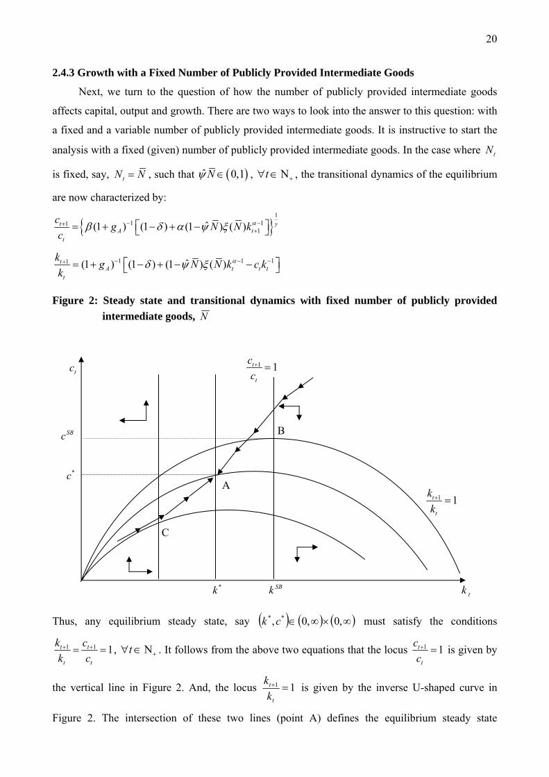
2.4.3 Growth with a Fixed Number of Publicly Provided Intermediate Goods

Next, we turn to the question of how the number of publicly provided intermediate goods

affects capital, output and growth. There are two ways to look into the answer to this question: with

a fixed and a variable number of publicly provided intermediate goods. It is instructive to start the

analysis with a fixed (given) number of publicly provided intermediate goods. In the case where tN

is fixed, say, tN N , such that ˆ 0,1N , t , the transitional dynamics of the equilibrium

are now characterized by:

1

1 111ˆ(1 ) (1 ) (1 ) ( )t

A tt

cg N N k

c

1 1 11 ˆ(1 ) (1 ) (1 ) ( )tA t t t

t

kg N N k c k

k

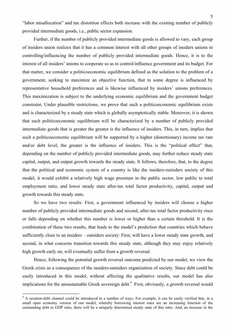
Figure 2: Steady state and transitional dynamics with fixed number of publicly provided

intermediate goods, N

Thus, any equilibrium steady state, say ,0,0, ** ck must satisfy the conditions

111

t

t

t

t

c

c

k

k, t . It follows from the above two equations that the locus 11

t

t

c

c is given by

the vertical line in Figure 2. And, the locus 11

t

t

k

k is given by the inverse U-shaped curve in

Figure 2. The intersection of these two lines (point A) defines the equilibrium steady state

1 1t

t

c

c

1 1t

t

k

k

Α

C

tc

SBc

*c

*k SBk tk

B

21

1

1* * * *

1

ˆ(1 ) ( )ˆ, , (1 ) ( ) ( )

(1 ) (1 ) AA

N Nk c N N k g k

g

. Also, it follows by the above

two equations that the transitional dynamics around this steady state are as indicated by the

directions of the arrows in Figure 2. Following standard arguments, it can be shown that there exists

a unique stable local trajectory to the steady state, to which the economy converges, monotonically.

Given any initial value of 0k , consumption “jumps” to the value that corresponds to this stable local

trajectory. Clearly, **,ck differs from the steady state of the Second Best (point B, say SBSB ck , ),

which lies to the north east of point A, by virtue of Corollary 2. And, for any given initial value of

0k , transitional dynamics (monotone convergence) will imply higher growth rates towards the

steady state of the Second Best, versus that of point A.

Now, we are interested in the steady state and the transitional dynamics for different values of

N . Consider first an increase in the relative wage premium (.) that does not come from a change

in N . Clearly, in this case, following Proposition 2, )(N will decrease. The 11

t

t

k

k locus will

drop and the 11

t

t

c

c locus will move left. The new steady state (illustrated by point C, in Figure 2)

will lie to the south west of **,ck . And, convergence to this steady state will imply slower growth.

Finally, if N increases, both loci will move in the direction )()ˆ1( NN moves. Where the new

steady state is going to be, is now ambiguous and depends on the way )()ˆ1( NN changes with

N . As the following proposition makes clear, for N sufficiently high, )()ˆ1( NN will decrease

with N . But, for N sufficiently low the opposite might be true.

Proposition 3 (Variety and Labor Misallocation Effects vs Tax Distortion Effect): Given

Assumptions 1 and 2, ˆ(1 ) ( )

0d N N

dN

for all

1 1,

ˆ1

bN

, such that:

(1 )(1 )

.ˆ (1 )(1 )

a bN

a b

And if,

1 (1 )(1 )

ˆ1 (1 )(1 )

b a b

a b

, there exists a sub-

interval 1

,1

bN

of

1 (1 )(1 )

,ˆ1 (1 )(1 )

b a b

a b

such that

ˆ(1 ) ( )0

d N N

dN

, for all N in this sub-interval.

Proof: In the Appendix.

22

Since, should be a relatively small number, the condition

1 (1 )(1 )

ˆ1 (1 )(1 )

b a b

a b

, puts an upper bound on , that seems reasonable for all

practical purposes. For that matter, we shall refer to

(1 )(1 )ˆ (1 )(1 )

a b

a b

as the threshold value

of N.

Proposition 3 can be illustrated in Figure 2, also. In this case, an increase in N that decreases

(increases) ˆ(1 ) ( )N N corresponds to a movement northeast (southwest) of point A, like point

C (B). Hence, in the case of a fixed number of publicly provided intermediate goods, an increase in

the number of these goods will have ambiguous effects on steady state output and growth towards

this steady state, as these effects will depend on the existing number of publicly provided

intermediate goods. However, the rationale for this nonlinearity is straightforward. For a relatively

low N, an increase in this number is associated with the dominance of the “variety” effect over the

combination of the “labor misallocation” and “tax distortion” effects. On the contrary, for a

relatively high N, an increase in this number is associated with the dominance of the combination of

the “labor misallocation” and “tax distortion” effects over the “variety” effect. For, as it can be

easily verified, the “variety” effect (“labor misallocation” and “tax distortion” effects) is decreasing

(are increasing) with N. The important implication of this result for the stylized facts of the

Introduction, will be discussed in the next section.

2.5 Government’s Objective Function

The stage has, now, been set to investigate the case of an endogenous income tax rate or an

endogenous number of publicly provided intermediate goods, tN . This income tax rate or number

of publicly provided intermediate goods, of course, must be decided by government. To do this, we

must specify the government’s objective function. Once the government objective function is

specified, the problem of government is a straightforward social planner’s problem. That is,

government decides on the income tax rate or the number of publicly provided intermediate goods,

so as to maximize its objective function, subject to the equilibrium laws of motion of the previous

section and the government budget constraint. The solution to this problem is the so called

politicoeconomic equilibrium.

First, we consider the case of the Median Voter Government, where the objective function of

government is the objective function of the representative household. Moreover in order to simplify,

henceforth, we consider the case where 1 . This is the case of logarithmic household

23preferences and full capital depreciation. Then, the equilibrium laws of motion (15) and (16),

reduce to:25

1ˆ(1 ) 1 ( ) ( ) a

t t t t t tc a N N N N k (19)

1

1 1ˆ1 1 ( ) ( ) a

t A t t t t tk a g N N N N k (20)

And, the temporal utility function of the representative household becomes logarithmic, so that the

objective function of the representative household and the so called Median Voter Government is

given by:

1 1 0 000

10

, ; , ln

ˆln (1 ) 1 ( ) ( )

MV tt t tt

t

t at t t t t

t

W k N k N c

a N N N N k

(21)

The problem of the Median Voter Government is to find a plan of the form 1 1 0,t t t

k N

so

as to maximize (21), subject to (20). We shall refer to the solution of this problem as the Median

Voter politicoeconomic equilibrium. It should be mentioned that the government budget constraint,

is such that choosing the number of intermediate goods in the beginning of period t+1 completely

determines the income tax rate. Thus, this politicoeconomic equilibrium assumes that there is a

commitment technology with respect to the income tax rate.26

Second, motivated by the Greek paradigm, where political parties and governments have been

dominated by unions and especially those of the greater public sector, we wish to consider a

situation where insiders’ unions are controlling government.27 We shall refer to this type of

government as Government of Insiders. But since in the equilibrium considered in the previous

subsection and, in particular, in the Nash equilibrium characterizing the outcome of the insiders’

unions strategic interaction, we assumed that each union takes the number of publicly provided

intermediate goods as given and beyond their control, it seems contradictory to argue that unions

cooperate to control/influence government.28 However, there is no such contradiction. Unions

“play” non-cooperatively vis-à-vis each other with respect to the wage rate, as an increase in the

wage rate set by each union affects positively its own utility but negatively each other union. This is

because, such an increase, due to the assumed gross complementarity, lowers labor demand facing

all other unions. But, have an incentive to cooperate with each other with respect to the income tax

25 To verify this, observe that (20) comes as an implication of the resource constraint (16) and that (19) satisfies the Euler condition (15). 26 Admittedly, here we avoid all problems that arise due to the lack of such commitment. See, e.g., Acemoglu (2009, Ch. 22), for what is referred to as the “hold up” problem. 27 Pertinent references are given in Kollintzas, et al. (2012). 28 This is what is referred to as “political elite” (see e.g., Acemoglu 2009, ch. 22). Elites are taken to make the political decisions and possibly engage in economic activities. In our case, the political elite consists of the members of insiders’ unions. Or, again, in Acemoglu’s terminology, we assume insiders’ unions to enjoy de facto political power.

24rate / the number of publicly provided intermediate goods. This is because a higher, say, income tax

rate, increases the number of publicly provided intermediate goods and increases the demand for

labor facing each union, also due to gross complementarity. Hence, all insiders’ unions have an

incentive to increase this tax rate (financing of the underlying infrastructure). For that matter,

unions’ interests are simultaneously to compete for wage premiums and cooperate for the number of

publicly provided intermediate goods. On the contrary, however, in a world of no insiders, there is

no need for such cooperation. We consider then the objective function of Insiders Government to be

a function of the sum of utilities of all insiders’ unions, ( )0

0 0

ln ( ) ( )tN

zt i it t t

t

w z w L z dz

, which in

the symmetric case reduces to:

1 1 0 000

0 1

, ; , ln ( ) ( )

( )ln ln

ˆ(1 ) 1 ( )

GI t at t t t tt

t

t tt

t t t t

W k N k N N N k

Nc

a N N N

(22)

where

(1 )/

( ) 1( )

( ) 1 ( )

tt

t t

v NN

N a b b N

(23)

The problem of the Government of Insiders is to find a plan of the form 1 1 0,t t t

k N

so as to

maximize (22), subject to (20). Clearly, then, Median Voter Government preferences depend on

consumption of the representative household only. But, Government of Insiders preferences depend

on a fraction, λ, of the representative household preferences; the function [ ( )]tN , which, as will

be shown in the proof of the next proposition, is an increasing and concave of the public sector

wage premium, ( )tN ; and government’s share of output, 1ˆ1 ( )t t tN N N . Interestingly,

as can be seen from (23), this last dependence occurs in such a way so as to offset the effect of the

government’s share of output incorporated in the consumption of the representative household.

Further, since we are interested in comparing societies with different politicoeconomic

structures, we wish to consider a hybrid of the government objective functions introduced above.

That is, following the political economy literature (see, e.g., Persson and Tabellini (2002), Ch. 7),

we consider a government that to some degree is influenced by representative household

preferences and is influenced, likewise, by insiders’ unions preferences. Thus, to avoid scale

problems, we consider a government that seeks to minimize a weighted average of the percentage

deviations of: (a) the welfare of the representative household from the welfare achieved under the

25solution of the Median Voter; and (b) the welfare of all insiders’ unions from the welfare achieved

under the solution of the Government of Insiders:29

1 1 0 0 1 1 0 00 0, ; , (1 ) , ; ,MV MV GI GI

t t t tt t

MV GI

W W k N k N W W k N k NW

W W

(24)

subject to the capital law of motion (20), where 1 0,1 is the relative influence of insiders’

unions on government. We shall refer to this problem as the problem of the Hybrid Government and

to the solution of this problem as the Hybrid politicoeconomic equilibrium. Clearly, for

1 ( 0 ), the Hybrid politicoeconomic equilibrium collapses to the Median Voter

(Government of Insiders) one. And, for an appropriate choice of (0,1) , the Hybrid equilibrium

represents a politicoeconomic equilibrium with any given degree of insiders influence over the

representative household in government decisions.

3. POLITICOECONOMIC EQUILIBRIUM

In this section we characterize the basic properties of the Hybrid politicoeconomic

equilibrium. The following is the main result of this paper.

Proposition 4 (Politicoeconomic equilibrium): Suppose [0,1) or 1 and

Assumption 3 1

ˆ(1 )(1 ) 1 (1 )ˆ1

(1 )

a b a b

a b

,

Then, given Assumptions 1 and 2:

(a) The Hybrid politicoeconomic equilibrium is characterized by (20) and

1

11 2 1 1

ˆ( ) ;

ˆ ˆ1 ( ) 1 ( )tt t t t t t

NN N N N N N

(25)

where

1 11

1 1

( ) ( )( ) ;

( ) ( )t t

tt t

N NN A B

N N

(26)

with (1 ) (1 ) (1 )

( , ) ,(1 ) (1 )

A B

.

(b) There exists a unique steady state, 1 1, (0, ) , ,

ˆ1

bk N x

associated with this

equilibrium, such that:

29 We prove below that the solutions to the Median Voter government and the Government of Insiders exist, so that (24) is well defined.

261

1ˆ(1 ) ( )

1

a

A

a N Nk

g

(27)

and N is the unique solution to:

1ˆ ˆ(1 ) ( ) ( 1)N N . (28)

(c) Moreover, an increase in the relative influence of insiders’ unions, 1 , would lead to a

higher steady state value, N .

Proof: In the Appendix.

Difference equations (20) and (25) describe the transitional dynamics of the politicoeconomic

equilibrium. Condition (25) is the key condition characterizing the transition of publicly provided

intermediate goods. These costs (benefits) are measured in terms of discounted utility decreases

(increases) associated with decreases (increases) of an equivalent amount in consumption, as the

amount of resources used to increase (decrease) the number of publicly provided intermediate

goods. It is instructive to consider, first, these costs and benefits in the simpler case of the Median

Voter politicoeconomic equilibrium. In this case, 1 , so that 1A and 0B ; and therefore,

11

1

( )( )

( )t

tt

NN

N

. Then, observe that an increase in the number of publicly provided intermediate

goods in any given period t on private capital will involve the following four effects: (i) A decrease

at the beginning of period 1t at a rate equal to 1ˆ[1 ( ) ] ( ) a

t t t t ta N N N N k , due to the

diversion of resources from private capital to the construction of the underlying infrastructure

associated with the increase in the number of publicly provided intermediate goods (i.e., new

infrastructure). (ii) A decrease at the beginning of period 2t at a rate equal to

2 1 1 1 1ˆ ˆ[1 ( ) ] ( ) at t t t ta N N N N k , due to the diversion of resources from private capital to

the maintenance of the new public sector infrastructure. (iii) An increase at the beginning of period

1t at a rate equal to 2 1 1 1 1ˆ[1 ( ) ] ( ) a

t t t t ta N N N N k , due to the ensuing non-diversion

of resources to the construction of this infrastructure, since it is already in place. (iv) An increase at

the beginning of period 1t at a rate equal to 12 1 1 1 1

1

( )ˆ[1 ( ) ] ( )

( )at

t t t t tt

Na N N N N k

N

,

due to the increase in TFP, brought about by the new infrastructure. In terms of discounted utility,

changes in consumption in period t are valued at

1 11

ˆ{(1 )[1 ( ) ] ( ) }t t at t t t t tc a N N N N k

and, changes in consumption in period 1t

are valued at 1 11

ttc . Hence, in terms of discounted utility, the costs and benefits associated with a

marginal increase in the number of publicly provided intermediate goods are

271

1ˆ[1 ( ) ] ( )t a

t t t t t tc a N N N N k 1 1

1 2 1 1 1 1ˆ ˆ[1 ( ) ] ( )t a

t t t t t tc a N N N N k

and

1 1 11 2 1 1 1 1 2 1 1 1 1

1

( )ˆ ˆ{ [1 ( ) ] ( ) [1 ( ) ] ( ) }

( )t a at

t t t t t t t t t t tt

Nc a N N N N k a N N N N k

N

respectively. Simplifying terms, it follows that (25), simply requires that these costs and benefits

should be equal at the margin. In the opposite case of the Government of Insiders politicoeconomic

equilibrium, where 0 , so that 1

Aa

1 a

Ba

, 1 1

11 1

( ) ( )1( ) (1 )

( ) ( )t t

tt t

N NN a

a N N

.

Then, observe that an increase in the number of publicly provided intermediate goods, in this case,

will involve exactly the four effects (i) – (iv) on private capital as in the case of the Median Voter

politicoeconomic equilibrium, but now these changes are valued differently. That is, in terms of

discounted utility, changes in consumption in period t and period 1t are, now, valued at

1ttc and 1 1

1t

tc , respectively. Moreover, discounted utility is, now, directly (i.e., not through

consumption) affected by four additional terms. First, in period 1t , by 1 1

1

( )

( )t t

t

N

N

, as the

increase in the number of publicly provided intermediate goods raises the public sector wage

premium, increasing the utility of insiders. Finally, the other three terms are opposite and

proportional (i.e., multiplied by (1 )a ) as the effects (i)-(iii) on private capital. This, as already

mentioned, is due to the fact that insiders preferences depend directly, positively, on governments,

share of output (i.e., through 11

ˆ{(1 )[1 ( ) ]}t t ta N N N ). Again, equating these costs and

benefits gives (25), for 0 . Clearly then, for (0,1) , (25) is a linear combination of its above

two special versions. Interestingly, the weights in this linear combination (i.e., A and B) depend not

only on , but on insiders union power, λ, and the technological parameters a and b.

Now, the stage has been set to look into the steady state of the politicoeconomic equilibrium.

This steady state is characterized by (27) and (28). Condition (28), that characterizes the steady

state number of publicly provided intermediate goods, is crucial. First, recall that Proposition 2

ensures that ( )

( )

N

N

is strictly positive. Likewise, it is shown that, given Assumptions 1 and 2,

( )

( )

N

N

is strictly positive. Moreover, it is shown that ( )

( )

N

N

approaches , as N approaches

1

1

a b

(i.e., ( )v N approaches 1) and approaches 0, as N approaches 1

(i.e., the endpoint of

its range). Further, it is shown that both ( )

ˆ(1 )( )

NN

N

and ( )

ˆ(1 )( )

NN

N

are strictly decreasing

and strictly concave in N. Clearly then, ˆ(1 ) ( )N N is positive, strictly decreasing, strictly

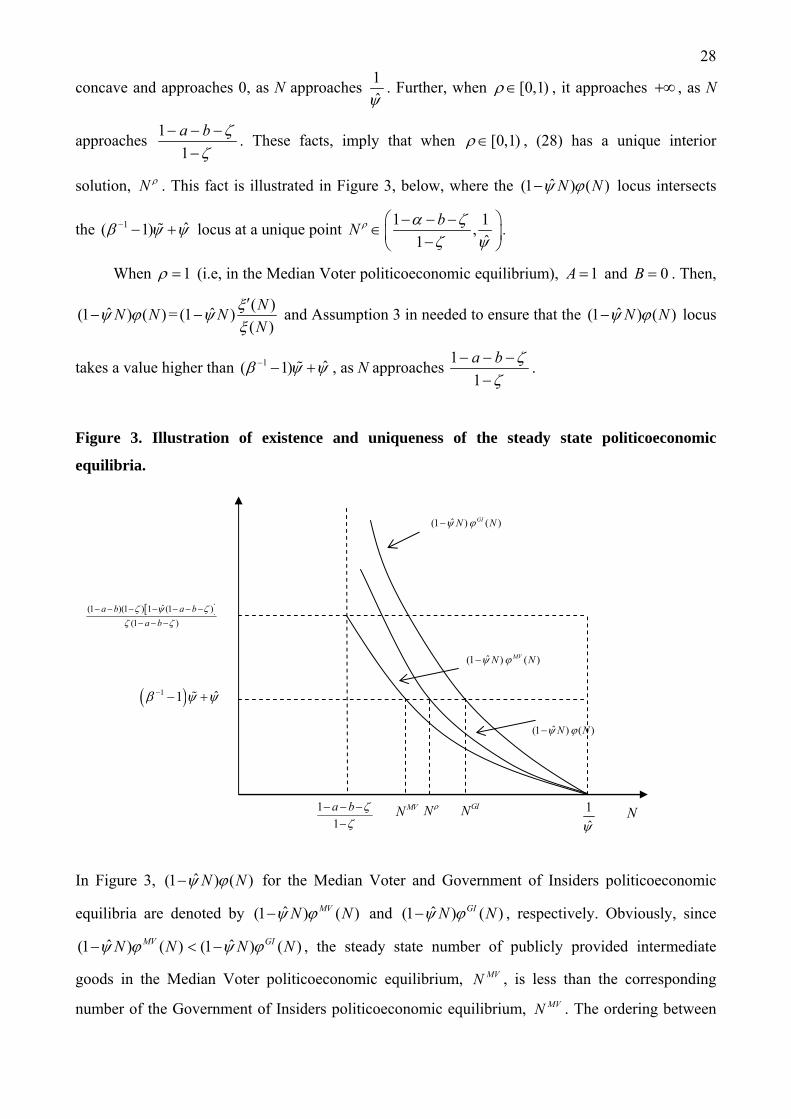
28

concave and approaches 0, as N approaches 1

. Further, when [0,1) , it approaches , as N

approaches 1

1

a b

. These facts, imply that when [0,1) , (28) has a unique interior

solution, N . This fact is illustrated in Figure 3, below, where the ˆ(1 ) ( )N N locus intersects

the 1 ˆ( 1) locus at a unique point 1 1

,ˆ1

bN

.

When 1 (i.e, in the Median Voter politicoeconomic equilibrium), 1A and 0B . Then,

ˆ(1 ) ( )N N =( )

ˆ(1 )( )

NN

N

and Assumption 3 in needed to ensure that the ˆ(1 ) ( )N N locus

takes a value higher than 1 ˆ( 1) , as N approaches 1

1

a b

.

Figure 3. Illustration of existence and uniqueness of the steady state politicoeconomic

equilibria.

In Figure 3, ˆ(1 ) ( )N N for the Median Voter and Government of Insiders politicoeconomic

equilibria are denoted by ˆ(1 ) ( )MVN N and ˆ(1 ) ( )GIN N , respectively. Obviously, since

ˆ(1 ) ( )MVN N ˆ(1 ) ( )GIN N , the steady state number of publicly provided intermediate

goods in the Median Voter politicoeconomic equilibrium, MVN , is less than the corresponding

number of the Government of Insiders politicoeconomic equilibrium, MVN . The ordering between

ˆ(1 ) ( )N N

ˆ(1 ) ( )GIN N

ˆ(1 )(1 ) 1 (1 )

(1 )

a b a b

a b

1 ˆ1

1

1

1

a b

MVN N GIN

ˆ(1 ) ( )MVN N

N

29GIN and MVN is a manifestation of the “political effect” mentioned in the Introduction. Recall that

the Median Voter solution incorporates the “labor misallocation” effect. So, steady state capital per

efficient household in the Median Voter solution is already lower than the Second Best (i.e., the no

wage premium but with distorting taxation Median Voter politicoeconomic equilibrium).30 Thus,

while the Median Voter social planner chooses the number of publicly provided intermediate goods

balancing (at the margin) the “variety” effect with the combination of the “labor misallocation” and

the “tax distortion” effects, the Government of Insiders chooses that number so as to balance the

same effects but with greater values for these effects, due to the utility gains from the public sector

wage premium and government’s share of output. For that matter, the Government of Insiders

chooses a greater number of intermediate goods than the Median Voter social planner. In fact, as

Part c of Proposition 4 makes clear, generally, an increase in insiders influence over government,

1 , would imply a higher steady state number of publicly provided intermediate goods.

Next, we turn on steady state capital, given by (27). Combining Propositions 3 and 4, it is

apparent that there is no direct answer to the question whether there will be a higher or a lower

steady state capital in the Median Voter social planner solution or the Government of Insiders

solution. Or, in general in the Hybrid politicoeconomic equilibrium, how steady state capital will

vary with an increase in the influence of insiders over government. In particular, for relatively low

numbers of steady state publicly provided intermediate goods, N , an increase in insiders influence

over government, leading to a higher number of those goods in the steady state, may entail higher

steady state capital and faster growth (i.e., growth along the convergence to the steady state). But,

for a relatively higher number of steady state publicly provided intermediate goods, N , a higher

number for these goods leads to lower steady state output and growth. We summarize this important

result in the following corollary.

Corollary 3: Consider two values of 1 , 1 and 1 , such that 1 1 .

Suppose that ,k N and ,k N are the steady states defined in Proposition 4 that

correspond to 1 and 1 , respectively. If ,N N

(1 )(1 ) 1,

ˆ ˆ(1 )(1 )

a b

a b

, so

that ˆ(1 ) ( )

0,d N N

dN

k k . And, if ,N N

1 (1 )(1 )

,ˆ1 (1 )(1 )

b a b

a b

so

that ˆ(1 ) ( )

0d N N

dN

, then k k .

30 In terms of Figure 3, the Second best corresponds to a solution with a

( )ˆ(1 )

( )

NN

N

locus that declines faster than

the one depicted in this figure.

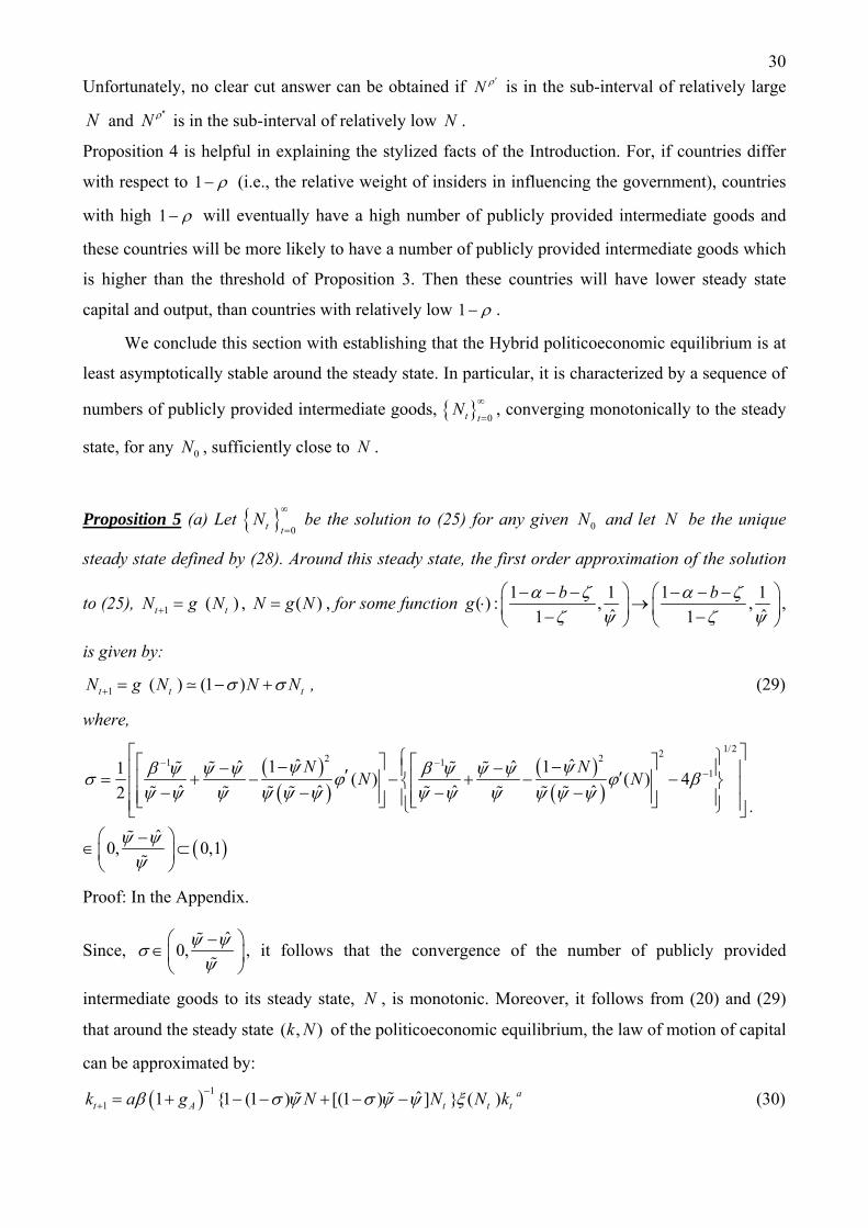
30

Unfortunately, no clear cut answer can be obtained if N is in the sub-interval of relatively large

N and N is in the sub-interval of relatively low N .

Proposition 4 is helpful in explaining the stylized facts of the Introduction. For, if countries differ

with respect to 1 (i.e., the relative weight of insiders in influencing the government), countries

with high 1 will eventually have a high number of publicly provided intermediate goods and

these countries will be more likely to have a number of publicly provided intermediate goods which

is higher than the threshold of Proposition 3. Then these countries will have lower steady state

capital and output, than countries with relatively low 1 .

We conclude this section with establishing that the Hybrid politicoeconomic equilibrium is at

least asymptotically stable around the steady state. In particular, it is characterized by a sequence of

numbers of publicly provided intermediate goods, 0t tN

, converging monotonically to the steady

state, for any 0N , sufficiently close to N .

Proposition 5 (a) Let 0t t

N

be the solution to (25) for any given 0N and let N be the unique

steady state defined by (28). Around this steady state, the first order approximation of the solution

to (25), 1 ( )t tN g N , ( )N g N , for some function 1 1 1 1

( ) : , ,ˆ ˆ1 1

b bg

,

is given by:

1 ( ) (1 )t t tN g N N N , (29)

where,

1/222 21 11

ˆ ˆ1 1ˆ ˆ1( ) ( ) 4

ˆ ˆ ˆ ˆ2

ˆ0, 0,1

N NN N

.

Proof: In the Appendix.

Since, ˆ

0,

, it follows that the convergence of the number of publicly provided

intermediate goods to its steady state, N , is monotonic. Moreover, it follows from (20) and (29)

that around the steady state ( , )k N of the politicoeconomic equilibrium, the law of motion of capital

can be approximated by:

1

1ˆ1 {1 (1 ) [(1 ) ] } ( ) a

t A t t tk a g N N N k (30)

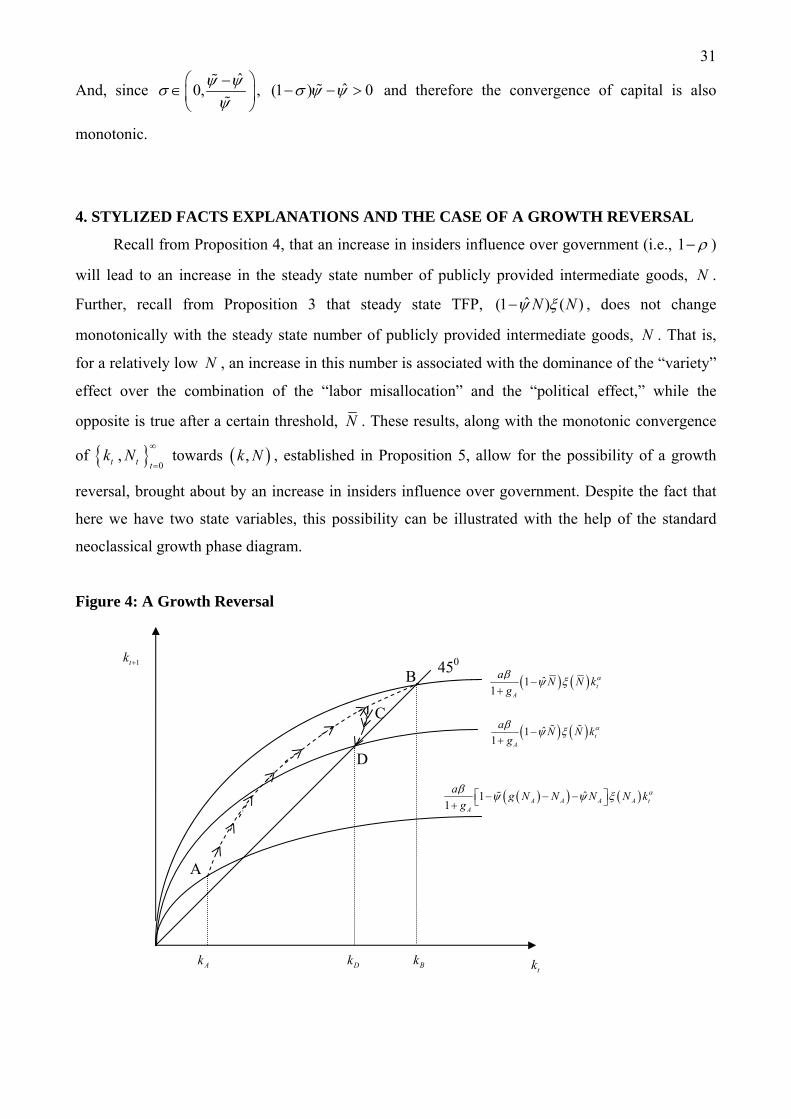
31

And, since ˆ

0,

, ˆ(1 ) 0 and therefore the convergence of capital is also

monotonic.

4. STYLIZED FACTS EXPLANATIONS AND THE CASE OF A GROWTH REVERSAL

Recall from Proposition 4, that an increase in insiders influence over government (i.e., 1 )

will lead to an increase in the steady state number of publicly provided intermediate goods, N .

Further, recall from Proposition 3 that steady state TFP, ˆ(1 ) ( )N N , does not change

monotonically with the steady state number of publicly provided intermediate goods, N . That is,

for a relatively low N , an increase in this number is associated with the dominance of the “variety”

effect over the combination of the “labor misallocation” and the “political effect,” while the

opposite is true after a certain threshold, N . These results, along with the monotonic convergence

of 0

,t t tk N

towards ,k N , established in Proposition 5, allow for the possibility of a growth

reversal, brought about by an increase in insiders influence over government. Despite the fact that

here we have two state variables, this possibility can be illustrated with the help of the standard

neoclassical growth phase diagram.

Figure 4: A Growth Reversal

ˆ11 t

A

aN N k

g

A

B

tk

450 1tk

ˆ11 A A A A t

A

ag N N N N k

g

C ˆ11 t

A

aN N k

g

Ak BkDk

D

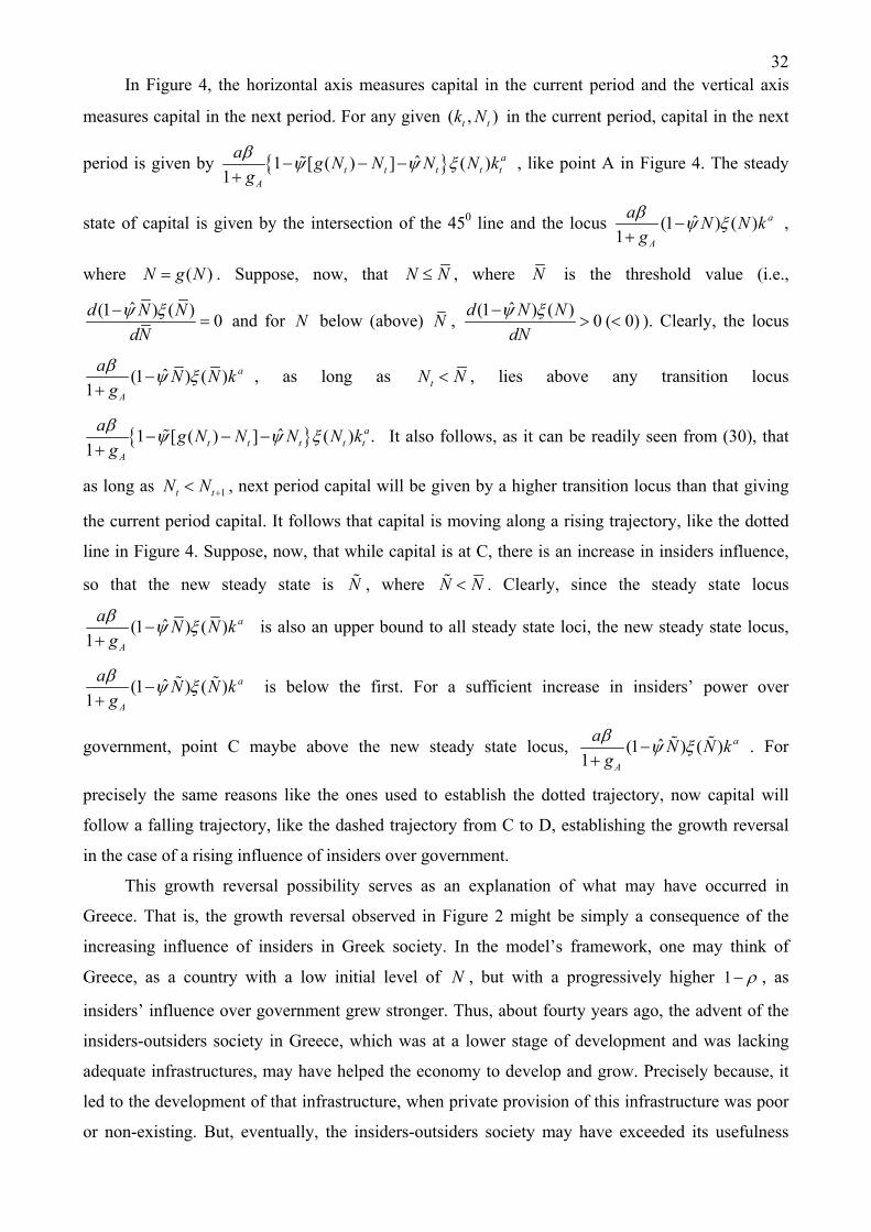
32In Figure 4, the horizontal axis measures capital in the current period and the vertical axis

measures capital in the next period. For any given ( , )t tk N in the current period, capital in the next

period is given by ˆ1 [ ( ) ] ( ) 1

at t t t t

A

ag N N N N k

g

, like point A in Figure 4. The steady

state of capital is given by the intersection of the 450 line and the locus ˆ(1 ) ( ) 1

a

A

aN N k

g

,

where ( )N g N . Suppose, now, that N N , where N is the threshold value (i.e.,

ˆ(1 ) ( )0

d N N

dN

and for N below (above) N ,

ˆ(1 ) ( )0 ( 0)

d N N

dN

). Clearly, the locus

ˆ(1 ) ( ) 1

a

A

aN N k

g

, as long as tN N , lies above any transition locus

ˆ1 [ ( ) ] ( ) . 1

at t t t t

A

ag N N N N k

g

It also follows, as it can be readily seen from (30), that

as long as 1t tN N , next period capital will be given by a higher transition locus than that giving

the current period capital. It follows that capital is moving along a rising trajectory, like the dotted

line in Figure 4. Suppose, now, that while capital is at C, there is an increase in insiders influence,

so that the new steady state is N , where N N . Clearly, since the steady state locus

ˆ(1 ) ( ) 1

a

A

aN N k

g

is also an upper bound to all steady state loci, the new steady state locus,

ˆ(1 ) ( ) 1

a

A

aN N k

g

is below the first. For a sufficient increase in insiders’ power over

government, point C maybe above the new steady state locus, ˆ(1 ) ( ) 1

a

A

aN N k

g

. For

precisely the same reasons like the ones used to establish the dotted trajectory, now capital will

follow a falling trajectory, like the dashed trajectory from C to D, establishing the growth reversal

in the case of a rising influence of insiders over government.

This growth reversal possibility serves as an explanation of what may have occurred in

Greece. That is, the growth reversal observed in Figure 2 might be simply a consequence of the

increasing influence of insiders in Greek society. In the model’s framework, one may think of

Greece, as a country with a low initial level of N , but with a progressively higher 1 , as

insiders’ influence over government grew stronger. Thus, about fourty years ago, the advent of the

insiders-outsiders society in Greece, which was at a lower stage of development and was lacking

adequate infrastructures, may have helped the economy to develop and grow. Precisely because, it

led to the development of that infrastructure, when private provision of this infrastructure was poor

or non-existing. But, eventually, the insiders-outsiders society may have exceeded its usefulness

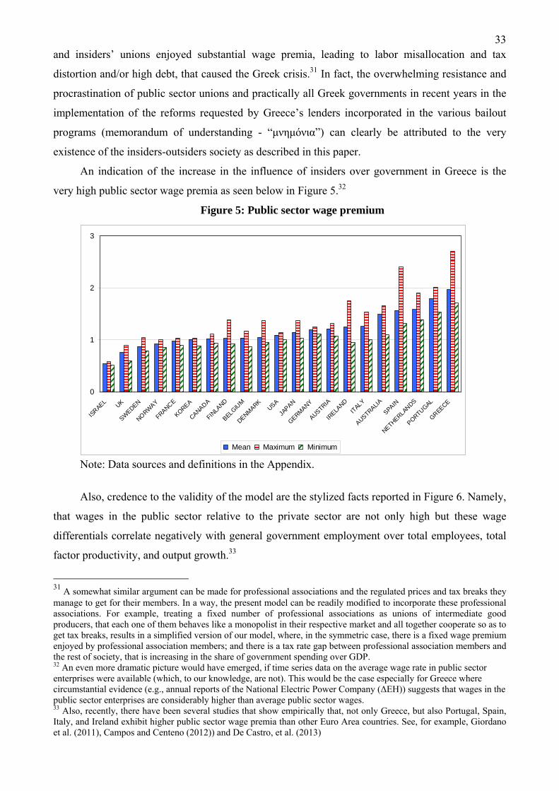
33and insiders’ unions enjoyed substantial wage premia, leading to labor misallocation and tax

distortion and/or high debt, that caused the Greek crisis.31 In fact, the overwhelming resistance and

procrastination of public sector unions and practically all Greek governments in recent years in the

implementation of the reforms requested by Greece’s lenders incorporated in the various bailout

programs (memorandum of understanding - “μνημόνια”) can clearly be attributed to the very

existence of the insiders-outsiders society as described in this paper.

An indication of the increase in the influence of insiders over government in Greece is the

very high public sector wage premia as seen below in Figure 5.32

Figure 5: Public sector wage premium

0

1

2

3

ISRAEL

UK

SWEDEN

NORW

AY

FRANCE

KOREA

CANADA

FINLA

ND

BELGIUM

DENMARK

USA

JAPAN

GERMANY

AUSTRIA

IRELA

ND

ITALY

AUSTRALIA

SPAIN

NETHERLANDS

PORTUGAL

GREECE

Mean Maximum Minimum

Note: Data sources and definitions in the Appendix.

Also, credence to the validity of the model are the stylized facts reported in Figure 6. Namely,

that wages in the public sector relative to the private sector are not only high but these wage

differentials correlate negatively with general government employment over total employees, total

factor productivity, and output growth.33

31 A somewhat similar argument can be made for professional associations and the regulated prices and tax breaks they manage to get for their members. In a way, the present model can be readily modified to incorporate these professional associations. For example, treating a fixed number of professional associations as unions of intermediate good producers, that each one of them behaves like a monopolist in their respective market and all together cooperate so as to get tax breaks, results in a simplified version of our model, where, in the symmetric case, there is a fixed wage premium enjoyed by professional association members; and there is a tax rate gap between professional association members and the rest of society, that is increasing in the share of government spending over GDP. 32 An even more dramatic picture would have emerged, if time series data on the average wage rate in public sector enterprises were available (which, to our knowledge, are not). This would be the case especially for Greece where circumstantial evidence (e.g., annual reports of the National Electric Power Company (ΔΕΗ)) suggests that wages in the public sector enterprises are considerably higher than average public sector wages. 33 Also, recently, there have been several studies that show empirically that, not only Greece, but also Portugal, Spain, Italy, and Ireland exhibit higher public sector wage premia than other Euro Area countries. See, for example, Giordano et al. (2011), Campos and Centeno (2012)) and De Castro, et al. (2013)

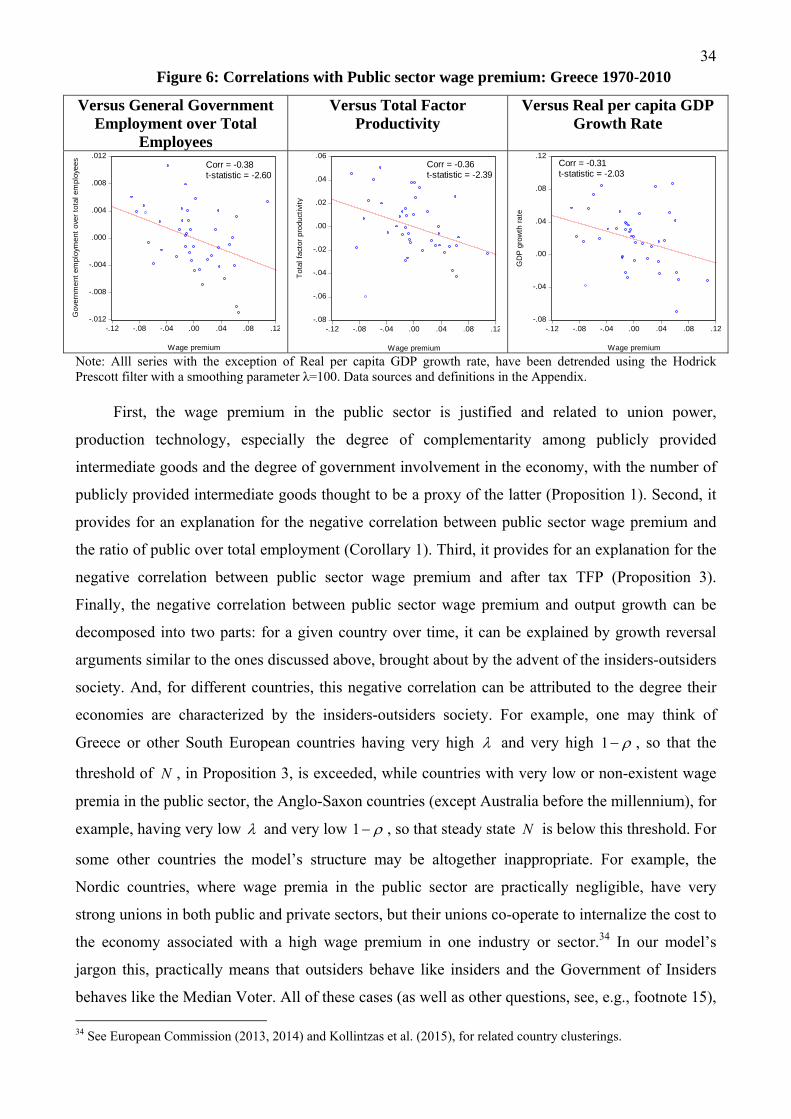
34Figure 6: Correlations with Public sector wage premium: Greece 1970-2010

Versus General Government Employment over Total

Employees

Versus Total Factor Productivity

Versus Real per capita GDP Growth Rate

-.012

-.008

-.004

.000

.004

.008

.012

-.12 -.08 -.04 .00 .04 .08 .12

Wage premium

Go

vern

me

nt

emp

loym

en

t o

ver

tota

l em

plo

yee

s

Corr = -0.38t-statistic = -2.60

-.08

-.06

-.04

-.02

.00

.02

.04

.06

-.12 -.08 -.04 .00 .04 .08 .12

Wage premium

Tot

al f

acto

r pr

oduc

tivi

ty

Corr = -0.36t-statistic = -2.39

-.08

-.04

.00

.04

.08

.12

-.12 -.08 -.04 .00 .04 .08 .12

Wage premium

GD

P g

row

th r

ate

Corr = -0.31t-statistic = -2.03

Note: Alll series with the exception of Real per capita GDP growth rate, have been detrended using the Hodrick Prescott filter with a smoothing parameter λ=100. Data sources and definitions in the Appendix.

First, the wage premium in the public sector is justified and related to union power,

production technology, especially the degree of complementarity among publicly provided

intermediate goods and the degree of government involvement in the economy, with the number of

publicly provided intermediate goods thought to be a proxy of the latter (Proposition 1). Second, it

provides for an explanation for the negative correlation between public sector wage premium and

the ratio of public over total employment (Corollary 1). Third, it provides for an explanation for the

negative correlation between public sector wage premium and after tax TFP (Proposition 3).

Finally, the negative correlation between public sector wage premium and output growth can be

decomposed into two parts: for a given country over time, it can be explained by growth reversal

arguments similar to the ones discussed above, brought about by the advent of the insiders-outsiders

society. And, for different countries, this negative correlation can be attributed to the degree their

economies are characterized by the insiders-outsiders society. For example, one may think of

Greece or other South European countries having very high and very high 1 , so that the

threshold of N , in Proposition 3, is exceeded, while countries with very low or non-existent wage

premia in the public sector, the Anglo-Saxon countries (except Australia before the millennium), for

example, having very low and very low 1 , so that steady state N is below this threshold. For

some other countries the model’s structure may be altogether inappropriate. For example, the

Nordic countries, where wage premia in the public sector are practically negligible, have very

strong unions in both public and private sectors, but their unions co-operate to internalize the cost to

the economy associated with a high wage premium in one industry or sector.34 In our model’s

jargon this, practically means that outsiders behave like insiders and the Government of Insiders

behaves like the Median Voter. All of these cases (as well as other questions, see, e.g., footnote 15),

34 See European Commission (2013, 2014) and Kollintzas et al. (2015), for related country clusterings.

35however, could be addressed by an extension of our model that incorporates a sector of privately

provided intermediate goods and their corresponding unions, along the lines of Cole and Ohanian

(2004).

5. CONCLUSIONS

In a synthesis of the insiders-outsiders labor market structure and the concept of an elite

government, we constructed a dynamic general equilibrium model of market and political power

interactions that can explain the growth reversal characterizing Greece in recent years. In this

country public sector unions act independently in their respective markets, but co-operate to

influence government policies, including those that affect public sector infrastructures. In so doing,

they increase taxes and/or debt to inefficient levels. Moreover, the model is consistent with several

stylized facts pertaining to the wage premium in the public sector, such as: the negative correlation

between the public sector wage premium, on the one hand, and the ratio of public sector

employment over total employment, total factor productivity, and output growth, on the other hand.

Finally, this model may be of interest to understand growth performance in other developed or

developing countries sharing similar institutional frictions with Greece.

ACKNOWLEDGEMENTS

We are grateful to Assar Lindbeck and Fabrice Collard for valuable comments. Dimitris

Papageorgiou and Vanghelis Vassilatos gratefully acknowledge co-financing of this research by the

European Union (European Social Fund — ESF) and Greek national funds through the Operational

Program “Education and Lifelong Learning” of the National Strategic Reference Framework

(NSRF) — Research Funding Program ARISTEIA II_Public Sector Reform, Research Grant, No

5328.

36REFERENCES

Acemoglu, D., (2006), Modeling Inefficient Institutions, in Advances in Economics and Econometrics, Theory and Applications, Ninth World Congress, Volume 1, R. Blundell, W. Newey, and T. Persson (Eds), Chapter 9, 341-380, Cambridge University Press.

Acemoglu, D., (2009), Introduction to Modern Economic Growth, Princeton University Press.

Acemoglu, D., Robinson, J.A., (2008), Persistence of power, elites, and institutions, American Economic Review, American Economic Association, vol. 98, 267-293.

Aghion, P., Howitt, P., (1998), Endogenous Growth Theory, MIT Press.

Alesina, A. and Giavazzi, F. (2004), The Economic Future of Europe, Journal of Economic Perspectives, vol. 18, 3-26.

Alogoskoufis, G. (1995), The two faces of Janus: institutions, policy regimes and macroeconomic performance in Greece, Economic Policy, 20, 147-192, April 1995.

Angeletos, G.M., Kollintzas, T., (2000), Rent seeking, corruption and growth, CEPR Discussion Paper No. 2464.

Ardagna, S., (2007), Fiscal policy in unionized labor markets, Journal of Economic Dynamics and Control, 31, pp. 1498-1534.

Becker, G.S., (1983), A theory of competition among pressure groups for political influence, Quarterly Journal of Economics, 98, 371-400.

Becker, G.S., (1985), Public policies, pressure groups and deadweight costs, Journal of Public Economics, 28, 330-347.

Blanchard, O., (2015), Greece: Past Critiques and the Path Forward, July 9, 2015, iMFdirect.

Blanchard, O., (2004), The economic future of Europe, Journal of Economic Perspectives, 18, 3-26.

Bosworth, B., Kollintzas, T., (2001), Economic Growth in Greece, in R.C. Bryant, N. C. Garganas, and G. S. Tavlas , Greece’s Economic Performance and Prospects (Bank of Greece and the Brookings Institution, 2001).

Bulow, J., Rogoff K., (2015), The modern Greek tragedy, VOX, CEPR’s Policy Portal, 10 June 2015.

Cawson, A., (1986), Corporatism and Political Theory, Oxford: Basil Blackwell.

Cole, H.L., Ohanian, L.E., (2004), New Deal policies and the persistence of the Great Depression: A General equilibrium analysis, Journal of Political Economy, 112(4), 779-816.

De Castro, F., Salto, M., Steiner, H., (2013), The gap between public and private wages: new evidence for the EU, European Economy Economic Papers 508, October 2013.

Esping-Andersen Gosta, (1990), The Three Worlds of Welfare Capitalism. Cambridge: Polity Press.

European Commission, (2014), Occasional Papers 190, April 2014, European Commission, Directorate-General for Economic and Financial Affairs.

European Commission, (2013), Industrial Relations in Europe 2012, European Commission, Directorate-General for Employment, Social Affairs and Inclusion.

Featherstone, K., (2008), ‘Varieties of Capitalism’ and the Greek case: explaining the constraints on domestic reform?, GreeSE Paper No 11, Hellenic Observatory Papers on Greece and Southeast Europe.

Fernandez-de-Cordoba, G., Perez, J., Torres, J., (2012), Public and private wages interaction in a general equilibrium model, Public Choice, 150, 309-326.

37Forni, L., Giordano, R., (2003), Employment in the public sector, CESIFO Working Paper, No. 1085.

Gogos, S.G., Mylonidis, N., Papageorgiou, D., Vassilatos, V., (2014), 1979–2001: A Greek great depression through the lens of neoclassical growth theory, Economic Modelling 36, 316-331.

Grossman, G.M., Helpman, E., (2002), Special Interest Politics, MIT Press.

Hall, P., Soskice, D., (2001), Varieties of Capitalism: The Institutional Foundations of Comparative Advantage, Oxford University Press, USA.

Kollintzas, T., Papageorgiou, D., Vassilatos, V., (2014), Some Stylized facts of Southern European capitalism, AUEB, mimeo, December 2014.

Krusell, P., Rios-Rull., J.V., (1996), Vested interests in a positive theory of stagnation and growth, The Review of Economic Studies, 63, 301-329.

Lindbeck, A., Snower, D.J., (1986), Wage setting, unemployment and Insider – Outsider relations, American Economic Review, 76, 235-9.

Lindbeck, A., Snower, D., (2001), Insiders versus Outsiders, Journal of Economic Perspectives, 15(1), 165-188.

Mc Donald, I.M., Solow, R.M., (1981), Wage bargaining and employment, American Economic Review, 71, 896-908.

Michas, T., (2011), Putting politics above markets: Historical background to the Greek crisis, Cato Institute Working Paper No. 5.

Molina, O., Rhodes, M., (2007), The Political Economy of Adjustment in Mixed Market Economies: A Study of Spain and Italy, in Hancke, B., Rhodes, M. and Thatcher, M. (Eds), Beyond Varieties of Capitalism, Oxford University Press.

Olson, M., (1965), The Logic of Collective Action: Public Goods and the Theory of Groups, Harvard University Press, Cambridge, MA.

Oswald, A., (1982), The microeconomic theory of trade unions, Economic Journal, 92, 576-95.

Parente, S.L., Prescott, E.C., (1994), Barriers to technology adoption and development, Journal of Political Economy, 102, 298-321.

Persson, T. and G. Tabellini (2002), Political Economics: Explaining Economic Policy, MIT Press.

Phelps, E.S., The Foundations of Greece’s Failed Economy, Project Syndicate, September 4, 2015. Link: http://www.project-syndicate.org/columnist/edmund-s--phelps.

Romer, P.M., (1990), Endogenous technological change, Journal of Political Economy, 98, 71-102.

Saint-Paul, G., (1996), Exploring the political economy of labor market institutions, Economic Policy, 23, 265-315.

Sargent, J., (1985), Corporatism and the European Community, in W. Grant, (Eds.), The Political Economy of Corporatism. London: Macmillan.

Schattschneider, E.E., (1935), Politics, Pressures and the Tariff, Prentice Hall, Englewood Cliffs, N.J.

Schmitter, P., (1977), Corporatism and Policy-Making in Contemporary Western Europe, London: Sage Publications.

Tullock, G., (2010), The economics of special privilege and rent seeking, Springer (reprint of 1989 edition).

Visser, J., (2013), Wage bargaining institutions – From crisis to crisis, European Economy, Economic Papers 448, April 2013.

Weingast, B.R., Shepsle, K., Johnsen, C., (1981), The political economy of benefits and costs: a neoclassical approach to distributive politics, Journal of Political Economy, 89, 642-664.

38APPENDIX

Proof of Proposition 2

Part a

Given Assumptions 1 and 2, ( ) 1v N , 1

,1

bN

. Therefore, it follows from

definition (18), that ( ) 0N , 1

,1

bN

. Fix 1

,1

bN N

and

consider as a function of ( ) 1v v N . That is, let:

(1 )(1 )1 1 1

1( ) ( ) ( ) (1 )1

a b bb a b a b

a

vN v N v b a b N

a b bv

And, therefore, given Assumptions 1 and 2,

(1 )(1 ) 11 1

2(1 )

(1 ) (1 )( ) (1 ) 0

1

a b bb a b a b

aN N

a b bv vv b a b N

v a b bv

.

Part b

Differentiate ( )N with respect to N , to get:

1 1 ( ) [ ( ) 1]

( ) ( )( ) 1 ( )t

a b bv N N v NN N

N v N a b bv N

. And, since 2

2

(1 ) ( )( )

a b v Nv N

N

,

( )( ) (1 ) ( )

NN a b N

N

(A.2.1)

where:

(1 ) ( ) ( ) 11( )

1 ( )

b a b v N v NN

N a b bv N

(A.2.2)

Clearly, then, given Assumptions 1 and 2,

( ) 0N

as ( ) 0N

, or as ( ) 0N

, where: 2 1

ˆ ˆ( ) ( ) [1 ( )] ( ) ( )a b

N v N v N v N v Nb

,

and, (1 )

ˆ( ) 0(1 )

Nv N

a b

. But, given Assumptions 1 and 2, ˆ[1 ( )] ( )v N v N ,

1,

1

bN

. To see this, note that ( ) 1v N , for 1

1

bN

. And, by

Proposition 1, it is strictly increasing, strictly concave, and approaches asymptotically

11

1 (1 )

, as N . On the other hand, ˆ[1 ( )]v N is

1 11

1 (1 )

for

39

1

1

bN

and increases at a constant rate, throughout

1,

1

b

. Therefore, given

Assumptions 1 and 2, ( ) 0N , 1

,1

bN

and hence ( ) 0N ,

1,

1

bN

.

Q.E.D.

Proof of Proposition 3

Note that:

ˆ(1 ) ( )0

d N N

dN

as

ˆ( ) ( )ˆ( ) 1

N N N

N N

Therefore, in view of (A.2.1) and (A.2.2), we have:

ˆ(1 ) ( )0

d N N

dN

as ( ), 0v N N

where

2 1( ), ( ) 1 ( ) ( ) ( )

a bv N N v N v N v N v N

b

and

ˆ ˆ1( )

ˆ ˆ(1 )(1 ) (1 )

N Nv N

a b N a b

Given Assumptions 1 and 2, 1

0 11

b

and in view of the facts that ˆ N and

0 1 , N is restricted to be in the interval 1 1 1

1 1, ,

ˆ1

bN N

N . Note, then, that if

2 2 2

(1 )(1 ) 1, ,

ˆ ˆ(1 )(1 )

a bN N N

a b

N , ( ) 0v N . And, since Assumptions 1 and 2

imply that 1( ) 1,v N N N , it follows that ( ), 0v N N , 1 2 1 2 2max , ,N N N N N N .

Hence, ˆ(1 ) ( )

0d N N

dN

, 1 2N N N . Further, observe that if 2 1N N , 1 2 1N N N and

there is no other case left to consider. Thus, suppose that 2 1N N and consider the case where

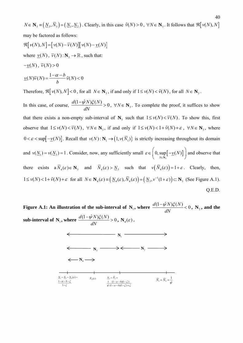
40

3 3 3 1 2, ,N N N N N N . Clearly, in this case ( ) 0v N , 3N N . It follows that ( ),v N N

may be factored as follows:

( ), ( ) ( ) ( ) ( )v N N v N v N v N v N

where ( )v N , 3( ) :v N N , such that:

( )v N , ( ) 0v N

1( ) ( ) ( ) 0

bv N v N v N

b

Therefore, ( ), 0v N N , for all 3N N , if and only if 1 ( ) ( )v N v N , for all 3N N .

In this case, of course, ˆ(1 ) ( )

0d N N

dN

, 3N N . To complete the proof, it suffices to show

that there exists a non-empty sub-interval of 3N such that 1 ( ) ( )v N v N . To show this, first

observe that 1 ( ) ( )v N v N , 3N N , if and only if 1 ( ) 1 ( )v N v N , 3N N , where

0 sup ( )v N . Recall that 1 1( ) : 1, ( )v N v NN is strictly increasing throughout its domain

and 1 3( ) ( ) 1v N v N . Consider, now, any sufficiently small 3

0, sup ( )N

v N

N

and observe that

there exists a 4 3( )N N and 4 3( )N N such that 4 ( ) 1v N . Clearly, then,

1 ( ) 1 ( )v N v N for all 14 4 4 3 3( ) ( ), ( ) , (1 )N N N N v N N (See Figure A.1).

Q.E.D.

Figure A.1: An illustration of the sub-interval of 1N , where ˆ(1 ) ( )

0d N N

dN

, 2N , and the

sub-interval of 1N , where ˆ(1 ) ( )

0d N N

dN

, 4 ( )N .

1N

3N 2N

1 3 4 ( )

1

1

N N N

b

4 ( )N 2 3

1 (1 )(1 )ˆ (1 )(1 )

N N

a b

a b

4N

1 2

1ˆ

N N

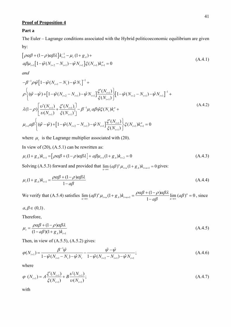
41Proof of Proposition 4

Part a

The Euler – Lagrange conditions associated with the Hybrid politicoeconomic equilibrium are given

by:

11

1 2 1 1 1 1

(1 ) (1 )

ˆ1 ( ) ( ) 0

t t A

at t t t t t

k g

a N N N N k

(A.4.1)

and

111

112 1 1 2 1 1

1

11 1

1 1

1 2 1

ˆ1 ( )

( )ˆ ˆ ˆ( ) 1 ( ) 1 ( )

( )

( ) ( )(1 ) ( )

( ) ( )

ˆ ˆ( ) 1 ( )

t t t

tt t t t t t

t

at tt t t

t t

t t t

N N N

NN N N N N N

N

N Na N k

N N

a N N N

11 1 1

1

( )( ) 0

( )at

t t tt

NN k

N

(A.4.2)

where t is the Lagrange multiplier associated with (20).

In view of (20), (A.5.1) can be rewritten as:

1 1 2(1 ) (1 ) (1 ) 0t A t t A tg k a g k (A.4.3)

Solving (A.5.3) forward and provided that 1lim ( ) (1 ) 0ut u A t uu

a g k gives:

1

(1 )(1 )

1t A tg ka

(A.4.4)

We verify that (A.5.4) satisfies 1

(1 )lim ( ) (1 ) lim ( ) 0

1u u

t u A t uu u

a g k aa

, since

, (0,1)a .

Therefore,

1

(1 )

(1 )(1 )tA ta g k

(A.4.5)

Then, in view of (A.5.5), (A.5.2) gives:

1

11 2 1 1

ˆ( ) ;

ˆ ˆ1 ( ) 1 ( )tt t t t t t

NN N N N N N

(A.4.6)

where

1 11

1 1

( ) ( )( ) ;

( ) ( )t t

tt t

N NN A B

N N

(A.4.7)

with

42(1 ) (1 ) (1 )

( , ) ( , )(1 ) (1 )

A B

. (A.4.8)

Part b

Let any steady state defined by:

1 1

1 1

... ... ;

... ... .

t t t

t t t

k k k k

N N N N

It follows from (20) and (A.5.6) that any steady state must satisfy:

1

1ˆ(1 ) ( )

1

a

A

a N Nk

g

(A.4.9)

and

1ˆ ˆ(1 ) ( ) ( 1)N N (A.4.10)

To prove the existence and uniqueness of the steady state, first note that the RHS of (A.4.10) is a

positive constant, 1 ˆ( 1) and the LHS in this equality is

ˆ(1 )N ( )N ( )

ˆ(1 )( )

NA N

N

+( )

ˆ(1 )( )

NB N

N

,where A>0 and B 0 , with B 0 if and only

if 1 . Consider first the function ( )

ˆ(1 )( )

NN

N

. It was shown in the proof of Proposition 2,

that, given Assumptions 1 and 2,

( )ˆ(1 )

( )

NN

N

=

1 ( )[ ( ) 1]ˆ(1 )(1 ) 0

( ) 1 ( )

bv N v Na b N

N v N a b bv N

, 1N N (A.4.11)

Further, recall from Proposition 1 that, given Assumptions 1 and 2:

2

2

(1 ) ( )( ) 0t

tt

a b NN

N

,

33

2 (1 ) 1 (1 ) ( )( ) 0t

tt

a b NN

N

, and

2 4

4

6 (1 ) 1 (1 ) ( )( ) 0

a b NN

N

. Also, recall from Proposition 2,that given

Assumptions 1 and 2,

2( ) (1 )(1 ) 1ˆ ˆ(1 ) 1 0

( ) (1 ) 1

N a b bN

N a b

, as 1N N and

( )ˆ(1 ) 0

( )

NN

N

as 1N N . Next, consider, the function ( )

ˆ(1 )( )

NN

N

, where

(1 )/

( ) 1( )

( ) 1 ( )t

v NN

N a b b N

. It follows that:

43

ˆ(1 )N

2

2

( ) (1 ) ( ) 1 (1 )ˆ(1 )

( ) ( )[ ( ) 1] 1 ( )

N a b v N bN

N N v N v N a b bv N

(A.4.12)

Using the above stated properties of ( )N , it follows by tedious but otherwise straightforward

algebra, that given Assumptions 1 and 2, ( ) / ( )

0d N N

dN

,

2

2

( ) / ( )0

d N N

dN

,

( )0

( )

N

N

,

( ) / ( )0

d N N

dN

,

2

2

( ) / ( )0

d N N

dN

1 1,N N N . Furthermore, it follows from (A.5.12)

that ( )

ˆ(1 )( )

NN

N

as 1N N and ( )

ˆ(1 ) 0( )

NN

N

as 1N N . Combining results, it

follows that: ˆ(1 ) ( ) 0N N ,ˆ[(1 ) ( )]

0d N N

dN

,

2

2

ˆ[(1 ) ( )]0

d N N

dN

1 1,N N N .

Moreover, ˆ(1 ) ( ) 0N N as 1N N . Furthermore, as long as 1 , ˆ(1 ) ( )N N as

1N N ; and when 1 , in which case ( )

ˆ ˆ(1 ) ( ) (1 )( )

NN N N

N

, Assumption 3 implies

that ˆ(1 ) ( )N N 2(1 )(1 )

(1 )

a b

a b

11ˆ ˆ(1 ) ( 1)

1

b

as 1N N . Hence,

under the stated assumptions, ˆ(1 ) ( )N N is continuous, positive, strictly decreasing and strictly

concave, 1 1,N N N . Further it takes a value greater than, 1 ˆ[( 1) ] 0 as 1N N ; and

takes the value 0, as 1N N . Therefore, ˆ(1 ) ( )N N takes the value 1 ˆ( 1) at a unique

point in the open interval 1 1,N N , N . And, therefore, (0, )k , defined by (A.4.9), is also

unique.

Part c

Note that affects ˆ(1 ) ( )N N only through A and B . Then, since both of these constants are

strictly decreasing functions of and ˆ(1 ) ( )N N is strictly increasing in both A and B, it is

immediate from Part b, that an increase in 1 increases the steady state value of value of N, N .

Q.E.D.

44Proof of Proposition 5

Let:

1

1 2 11 2 1 1

ˆ, ,

ˆ ˆ1 1t t t tt t t t t t

h N N N NN N N N N N

(A.5.1)

Then,

1 2, , 0t t th N N N (A.5.2)

is equivalent to (A.4.6). And,

, , 0h N N N (A.5.3)

is equivalent to (A.4.10).

Taking a first order approximation of 1 2, ,t t th N N N around , ,h N N N , we have:

1 2

3 2 2 1 1

, , , ,

, , , , , , 0

t t t

t t t

h N N N h N N N

h N N N N N h N N N N N h N N N N N

(A.5.4)

where , ,ih N N N , 1, 2,3i denote the partial derivatives of h with respect to its first, second

and third argument, respectively, evaluated at , ,N N N . In view of (A.5.3), (A.5.4) yields:

21 2

2 12 2 2

12

ˆ ˆ( )

ˆ ˆ ˆ1 1 1

ˆ0

ˆ1

t t

t

N N N N NN N N

N NN

(A.5.5)

It follows that the characteristic equation associated with (A.5.5) is:

212 1

ˆ1ˆ( ) 0

ˆ ˆ

NN

This equation has two roots, ˆ

0, (0,1)

and 1( ) 1 . Then, since tN is restricted to

be in the interval 1 1

,ˆ1

b

, the unique solution of (A.5.5) is given by:

1t tN N N N (A.5.6)

where:

1/222 21 11

ˆ ˆ1 1ˆ ˆ1( ) ( ) 4

ˆ ˆ ˆ ˆ2

N NN N

Q.E.D.

45DATA APPENDIX

The data set includes twenty-one OECD individual countries (Australia, Austria, Belgium,

Denmark, Finland, France, Germany, Greece, Italy, Ireland, Israel, Korea, Netherlands, Portugal,

Spain, Canada, Japan, Norway, Sweden, UK and US.), as well as time series for total OECD

countries and Euro area-19 countries. Data are yearly and cover a maximum time span from 1970 to

2010. Our main data source is the OECD Economic Outlook no. 90. Missing values for some

specific time periods/variables have been completed from the OECD Economic Outlook no. 88, 86,

85 and AMECO. Other data sources are the OECD Aggregate National Accounts and OECD.stats.

Variable Source

Real Gross Domestic Product (per head, constant prices, constant PPPs)

OECD.stat

Total compensation of employees OECD Economic Outlook and OECD Aggregate National Accounts Government final wage consumption expenditure1 OECD Economic Outlook and AMECO

Dependent employment - Total economy (Total employees)2

OECD Economic Outlook

Dependent employment in the private sector (Private sector employees)2 OECD Economic Outlook

General government employment3 OECD Economic Outlook

Total compensation of employees in the private sector

Own calculations (Total compensation of employees minus government final wage consumption expenditure)

Compensation rate in the private sector Own calculations (Total compensation of employees in the private sector divided by private sector employees)

Compensation rate in the public sector Own calculations (Government final wage consumption expenditure divided by government employment)

Public sector wage premium Own calculations (Compensation rate in the public sector divided by the compensation rate in the private sector)

Total factor productivity-Total economy AMECO

Output gap Own calculations (Gap between Real GDP in PPP values and Hodrick-Prescott trend divided by H-P filter)

Real Gross Domestic Product - Greece AMECO Population 15-64 - Greece OECD Economic Outlook Notes:

1. For Australia, government final wage consumption is computed as *CGW WSSS WSSE EEP ,

where WSSS is total compensation of employees, WSSE is the compensation rate in the private

sector and EEP is dependent employment in the private sector.

2. For Germany and Korea, total dependent employment, EE , and dependent employment in the

private sector, EEP , are respectively computed from the following relationships: /WSST WSSS EE

and ( ) /WSSE WSSS GCW EEP , where WSST is the compensation rate of the total economy, WSSE is

the compensation rate in the private sector, WSSS is total compensation of employees, and GCW is

government final wage consumption expenditure. For Israel, EE is computed as EE ET ES ,

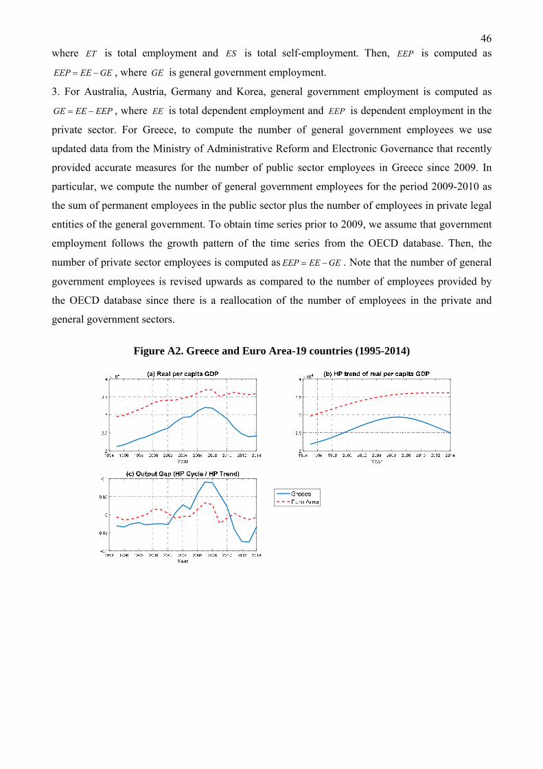
46where ET is total employment and ES is total self-employment. Then, EEP is computed as

EEP EE GE , where GE is general government employment.

3. For Australia, Austria, Germany and Korea, general government employment is computed as

GE EE EEP , where EE is total dependent employment and EEP is dependent employment in the

private sector. For Greece, to compute the number of general government employees we use

updated data from the Ministry of Administrative Reform and Electronic Governance that recently

provided accurate measures for the number of public sector employees in Greece since 2009. In

particular, we compute the number of general government employees for the period 2009-2010 as

the sum of permanent employees in the public sector plus the number of employees in private legal

entities of the general government. To obtain time series prior to 2009, we assume that government

employment follows the growth pattern of the time series from the OECD database. Then, the

number of private sector employees is computed as EEP EE GE . Note that the number of general

government employees is revised upwards as compared to the number of employees provided by

the OECD database since there is a reallocation of the number of employees in the private and

general government sectors.

Figure A2. Greece and Euro Area-19 countries (1995-2014)