
Ομιλία κ. Μπεζαντάκου Δανάης- Managing Director, Navigator Shipping Consultants LTD
Managing Risk in the Supply Chain
David Simchi-Levi
Joint work with Xin Chen, Victor Martínez-de-Albéniz, Melvyn Sim, Peng Sun
Approaches to Risk Management
2
Economics literatureVon Neumann-Morgenstern utilities
Expected utility E{U(Π)}
Finance literatureCapital Asset Pricing Model (CAPM)
Markowitz Mean-Variance tradeoff E{Π}- kVar{Π}Portfolio Approach
Linking Economics with Finance
3
WhenThe utility function is quadratic
ORThe utility is CARA* [U(Π)=-exp(-r Π)] and Π is normally distributed
ThenExpected utility maximization is equivalent to mean-variance objective maximization
*CARA: Constant Absolute Risk Averse
Operations Management
4
Academia:Traditional models focus on maximizing expected profit
Practice:Significant increase in the level of risk faced by many companies
Examples: Cisco, Apple, Sony…
Outline
5
Literature Review
Portfolio Contracts
Risk-Averse Inventory Models
Conclusion
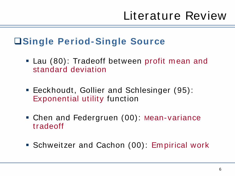
Literature Review
6
Single Period-Single Source
Lau (80): Tradeoff between profit mean and standard deviation
Eeckhoudt, Gollier and Schlesinger (95):Exponential utility function
Chen and Federgruen (00): Mean-variance tradeoff
Schweitzer and Cachon (00): Empirical work
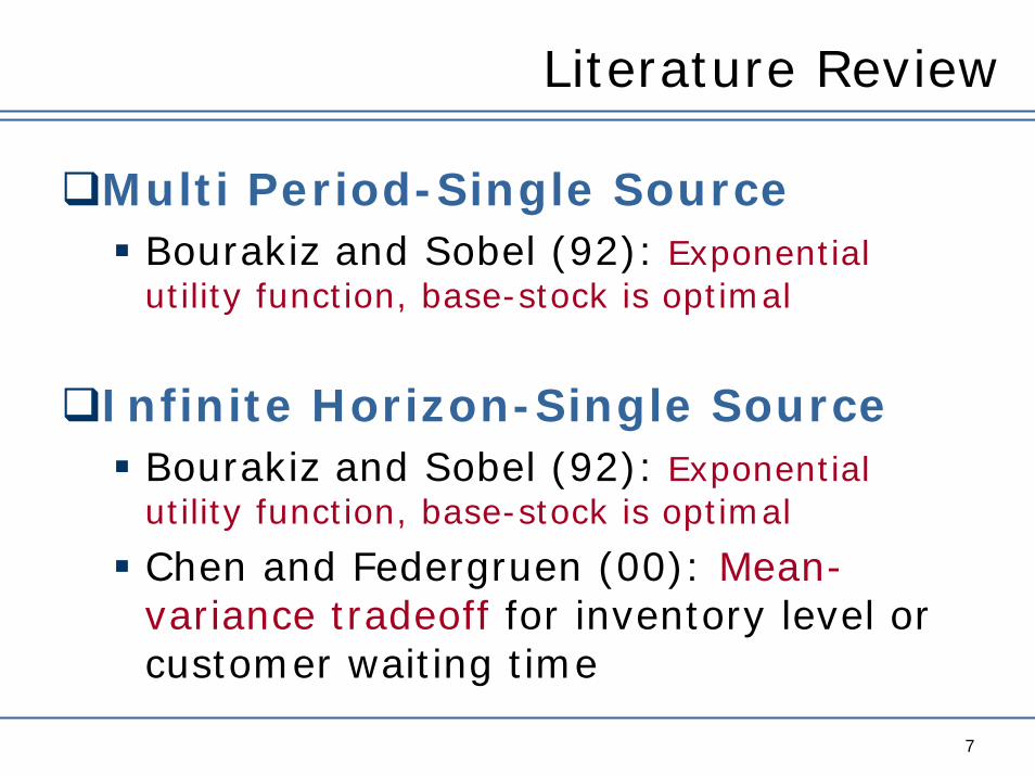
Literature Review
7
Multi Period-Single SourceBourakiz and Sobel (92): Exponential utility function, base-stock is optimal
Infinite Horizon-Single SourceBourakiz and Sobel (92): Exponential utility function, base-stock is optimal
Chen and Federgruen (00): Mean-variance tradeoff for inventory level or customer waiting time
Outline
8
Literature Review
Portfolio Contracts
Risk-Averse Inventory Models
Conclusion
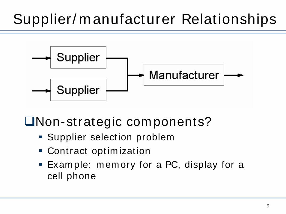
Supplier/manufacturer Relationships
9
Non-strategic components?Supplier selection problemContract optimizationExample: memory for a PC, display for a cell phone
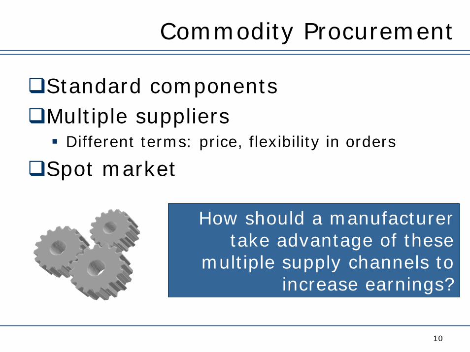
Commodity Procurement
10
Standard componentsMultiple suppliers
Different terms: price, flexibility in orders
Spot market
How should a manufacturer take advantage of these
multiple supply channels to increase earnings?
The Impact of Uncertainty
11
Demand uncertaintyFixed commitment is cheaper but creates high inventory riskFlexible commitment allows to match supply and demand but more expensive
Spot market uncertaintyContracting creates price risk
Modeling Example
12
3 demand scenariosHighest – mean – lowest
Available sourcingFixed commitment contractFlexible commitment contract (or option)Spot market
What should the purchasing strategy be?
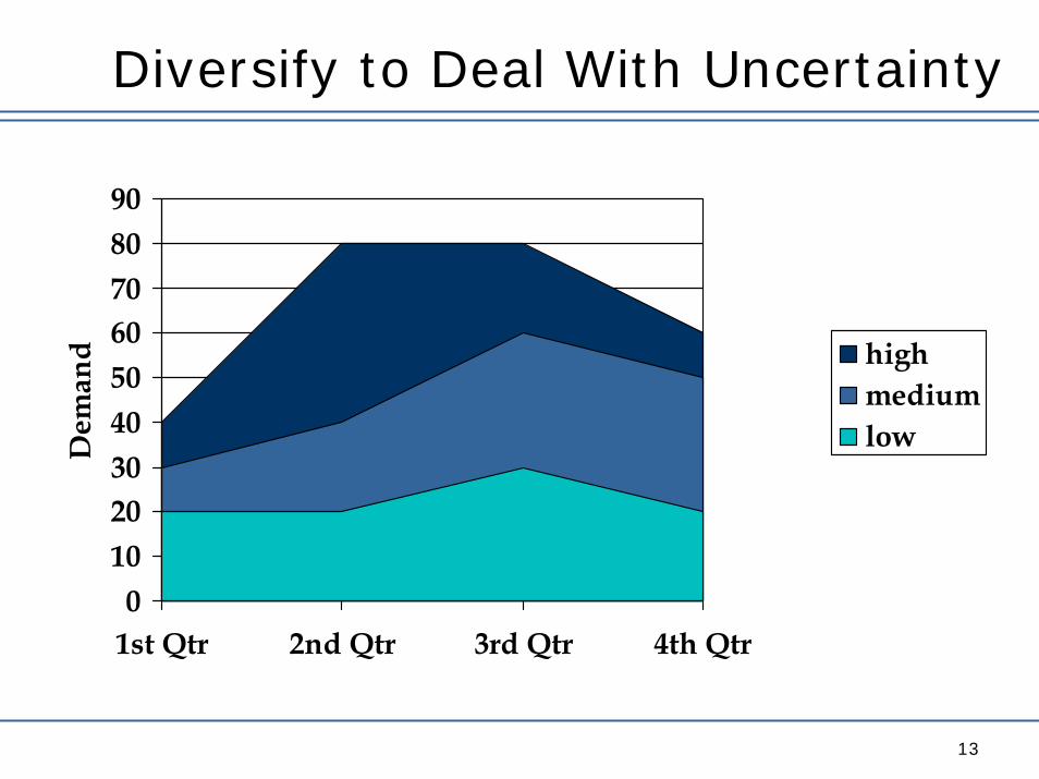
Diversify to Deal With Uncertainty
13
0102030405060708090
1st Qtr 2nd Qtr 3rd Qtr 4th Qtr
Dem
and high
mediumlow
Portfolio Contracts: Outline
14
ModelTwo problems
Optimal replenishment policiesOptimal contract purchasing
Mean-Variance TradeoffSuppliers Competition
Contracts Used Often in Practice
15
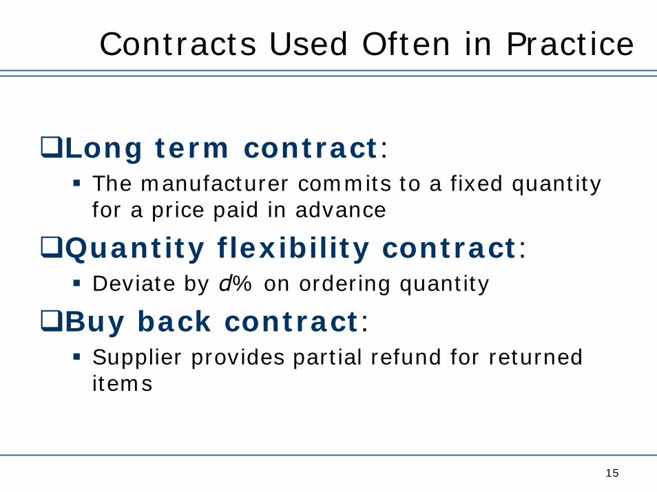
Long term contract:The manufacturer commits to a fixed quantity for a price paid in advance
Quantity flexibility contract:Deviate by d% on ordering quantity
Buy back contract:Supplier provides partial refund for returned items
Option Contract
16
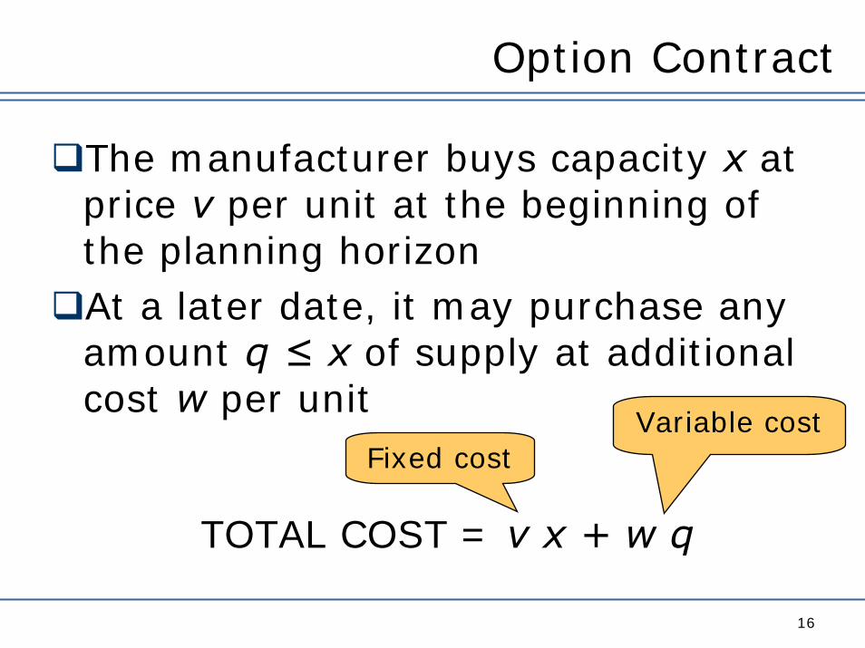
The manufacturer buys capacity x at price v per unit at the beginning of the planning horizonAt a later date, it may purchase any amount q ≤ x of supply at additional cost w per unit
TOTAL COST = v x + w q
Fixed costVariable cost
Portfolio Contract
17
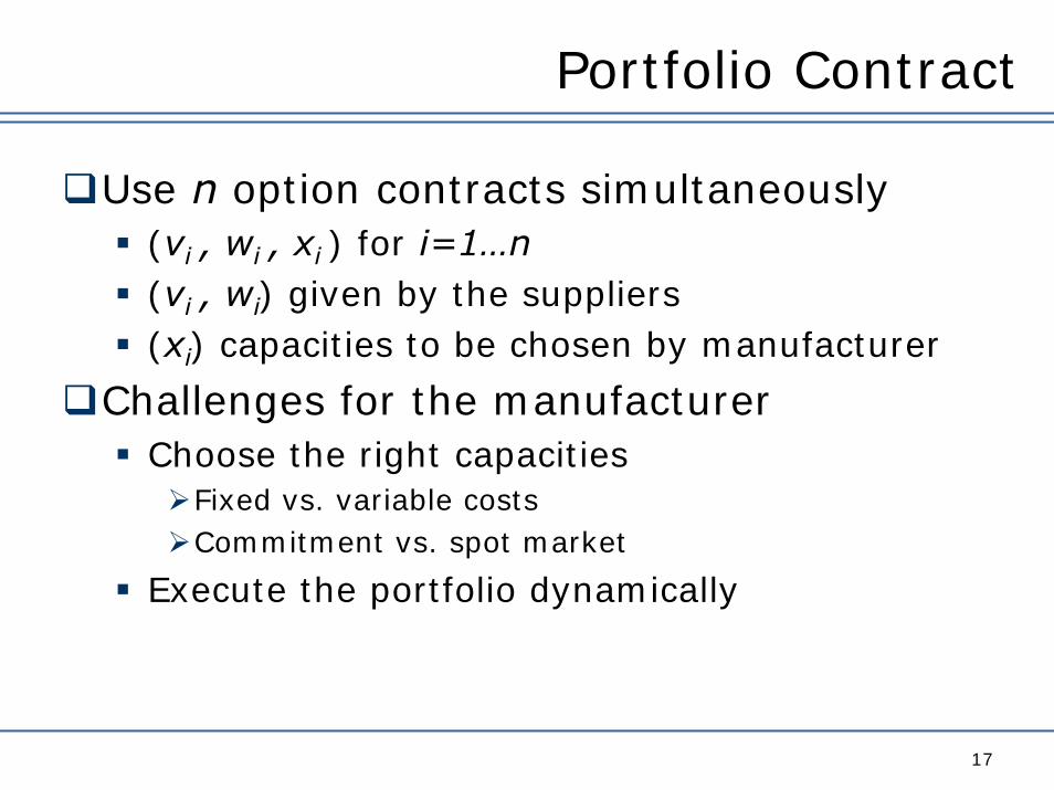
Use n option contracts simultaneously(vi , wi , xi ) for i=1…n(vi , wi) given by the suppliers(xi) capacities to be chosen by manufacturer
Challenges for the manufacturerChoose the right capacities
Fixed vs. variable costsCommitment vs. spot market
Execute the portfolio dynamically
Sequence of Events
18
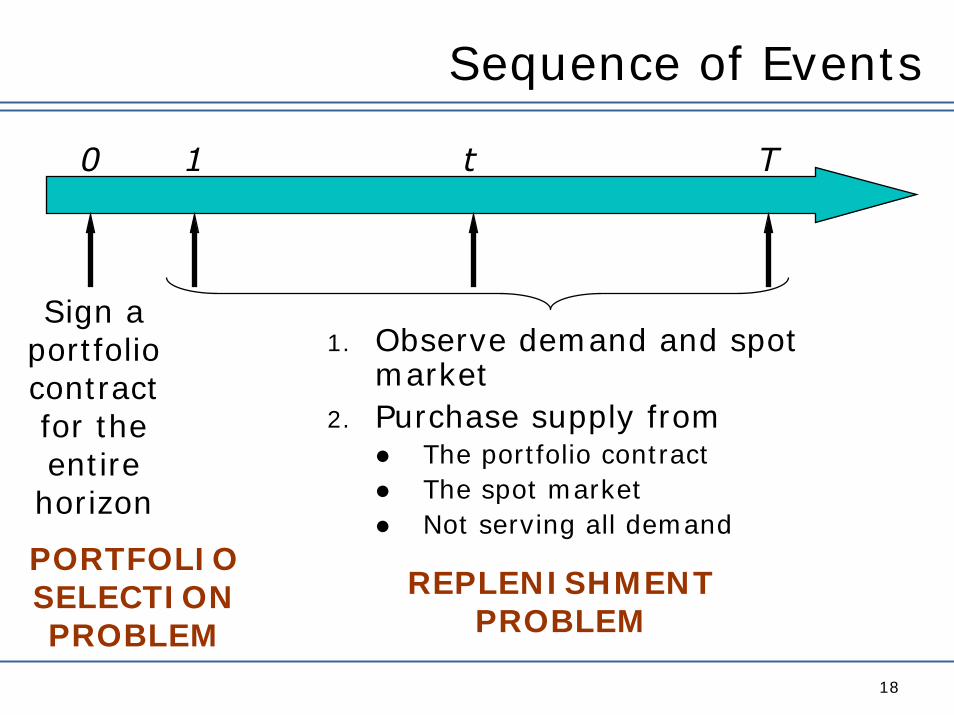
0 t1 T
Sign a portfolio contract for the entire
horizon
1. Observe demand and spot market
2. Purchase supply fromThe portfolio contractThe spot marketNot serving all demand
PORTFOLIO SELECTION PROBLEM
REPLENISHMENT PROBLEM
The Model
19
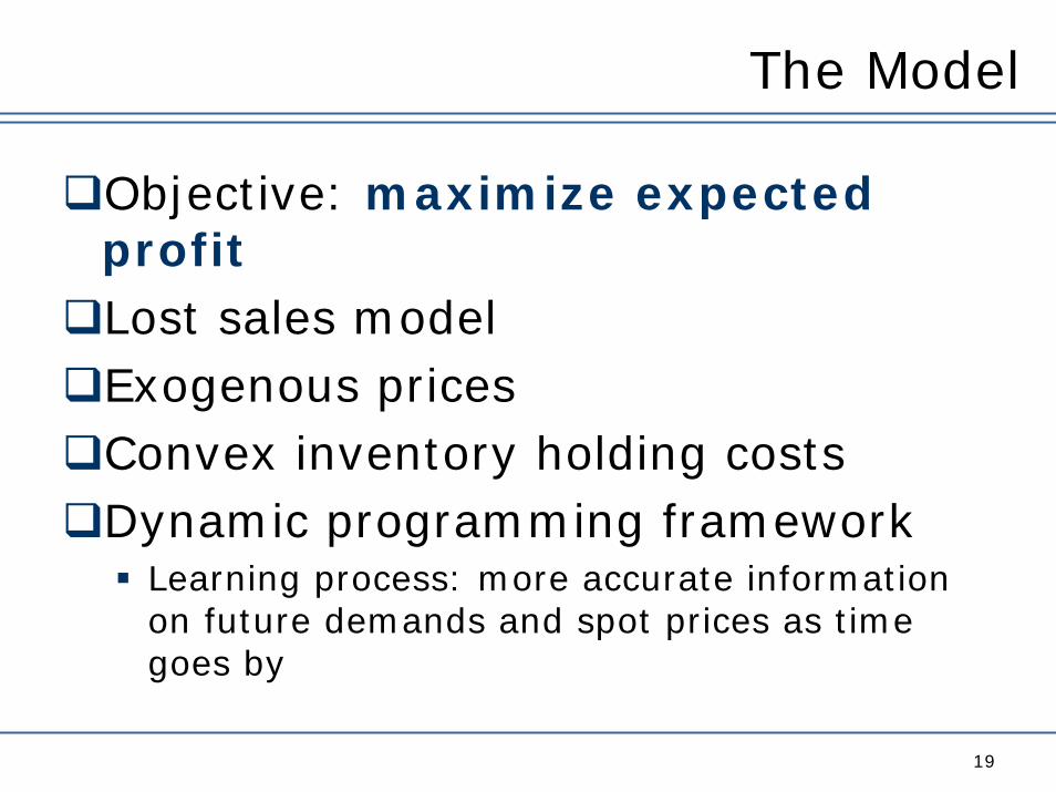
Objective: maximize expected profitLost sales modelExogenous pricesConvex inventory holding costsDynamic programming framework
Learning process: more accurate information on future demands and spot prices as time goes by
Spot Market Modeling
20
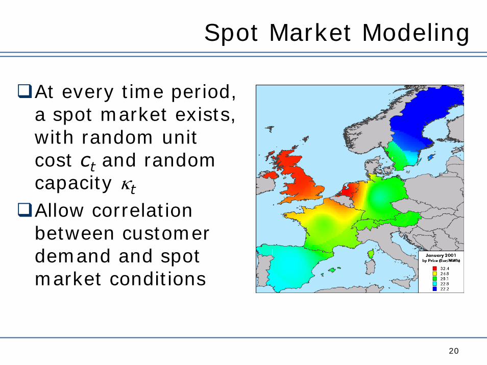
At every time period, a spot market exists, with random unit cost ct and random capacity κt
Allow correlation between customer demand and spot market conditions
Modeling the Portfolio
21
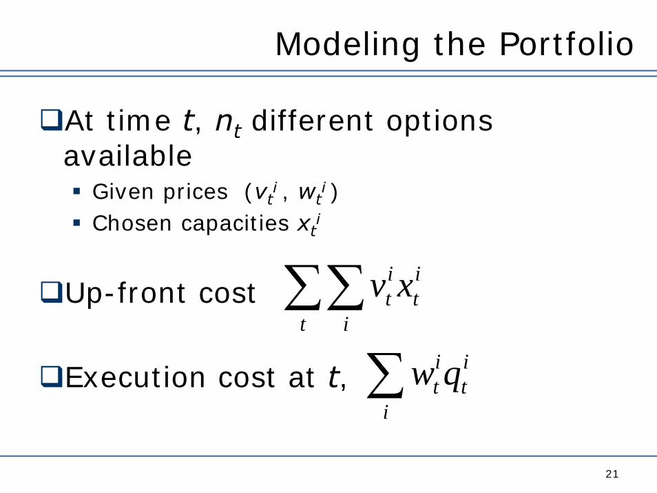
At time t, nt different options available
Given prices (vti , wt
i )Chosen capacities xt
i
Up-front cost
Execution cost at t,
∑∑t i
it
it xv
∑i
it
it qw
DP Formulation
22
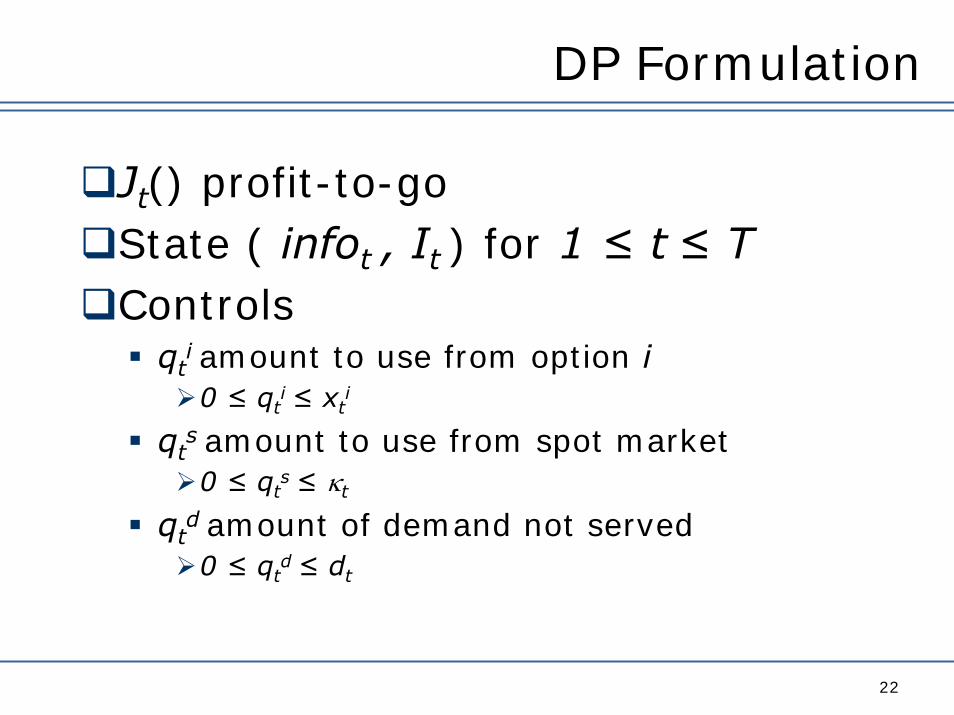
Jt() profit-to-goState ( infot , It ) for 1 ≤ t≤ TControls
qti amount to use from option i0 ≤ qt
i≤ xti
qts amount to use from spot market0 ≤ qt
s≤ κt
qtd amount of demand not served0 ≤ qt
d≤ dt
Characterizing the Profit-to-go
23
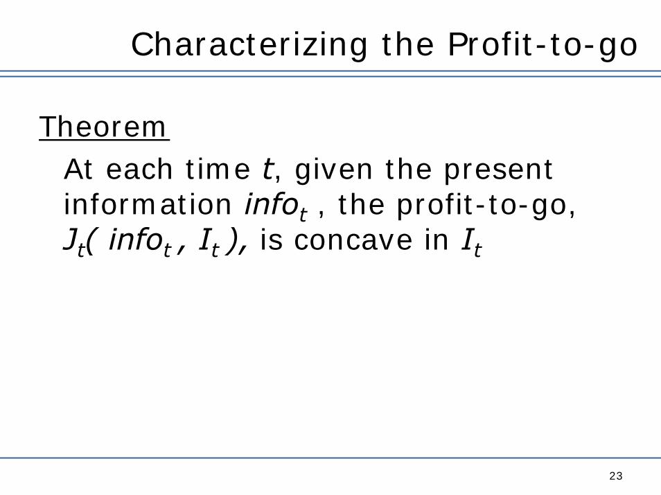
TheoremAt each time t, given the present information infot , the profit-to-go, Jt( infot , It ), is concave in It
The Structure of the Optimal Policy
24
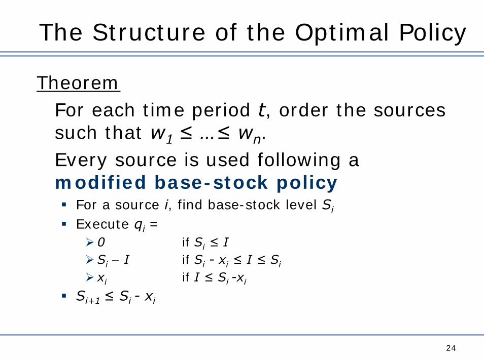
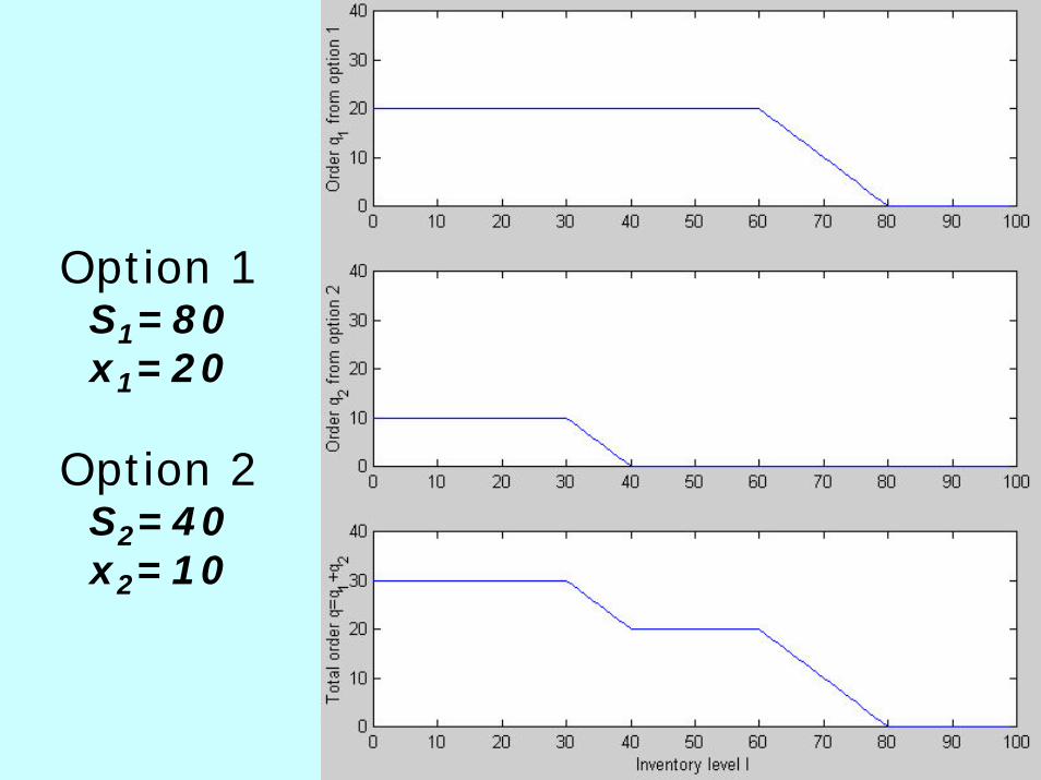
TheoremFor each time period t, order the sources such that w1 ≤ …≤ wn.Every source is used following a modified base-stock policy
For a source i, find base-stock level Si
Execute qi =0 if Si ≤ ISi – I if Si - xi ≤ I ≤ Si
xi if I ≤ Si -xi
Si+1 ≤ Si - xi
25
Option 1S1=80x1=20
Option 2S2=40x2=10
Portfolio Selection Problem
26
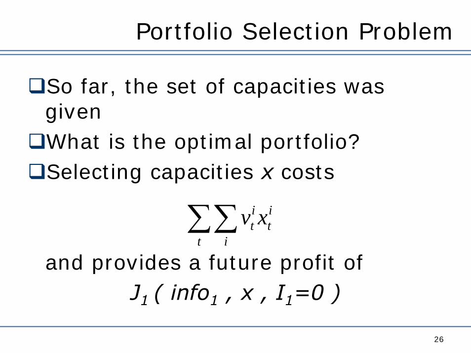
So far, the set of capacities was givenWhat is the optimal portfolio?Selecting capacities x costs
and provides a future profit ofJ1 ( info1 , x , I1=0 )
∑∑t i
it
it xv
Portfolio Selection Problem
27
TheoremThe function J1(info1, x, I1=0) is concave in x ≥ 0
CorollarySelecting the optimal capacities is a concave maximization problem
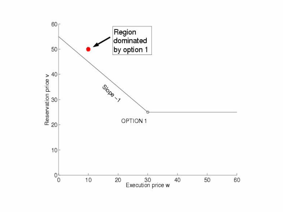
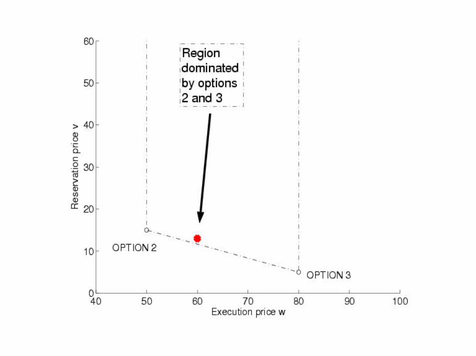
Characterizing Optimal Portfolios
28
Non-attractive contractsContracts dominated by the spot market
E[(SPOT-w)+] ≤ vContracts dominated by other options
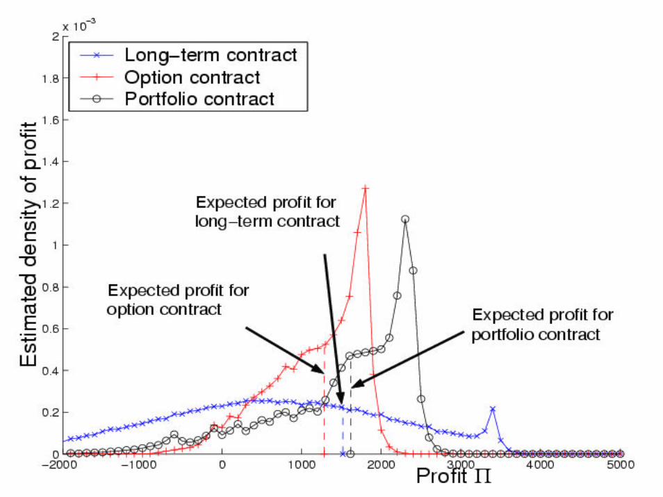
Numerical Results
31
2 contractsLong term contract [v1=7, w1=0]Option contract [v2=2, w2=7]
Comparison of profit distributionThrough Montecarlo simulationBetween one contract only and a portfolio
Insights from variances
Outline
33
Portfolio contracts modelingTwo problems
Optimal replenishment policiesOptimal contract purchasing
Mean-Variance TradeoffSuppliers Competition
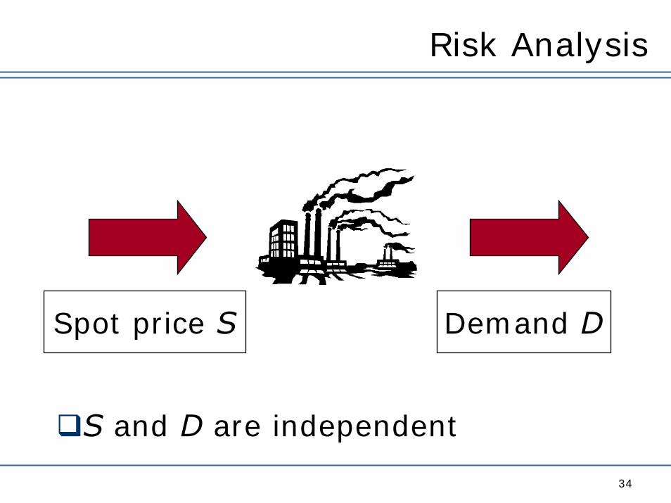
Risk Analysis
34
Demand DSpot price S
S and D are independent

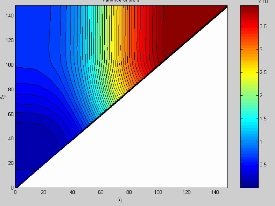
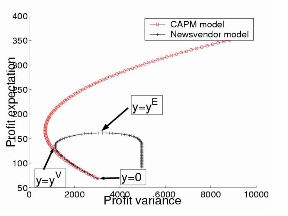
Profit Variance
35
TheoremThe lower-level sets of the profit variance are connected.
Any portfolio that locally minimizesthe variance is a global minimizer
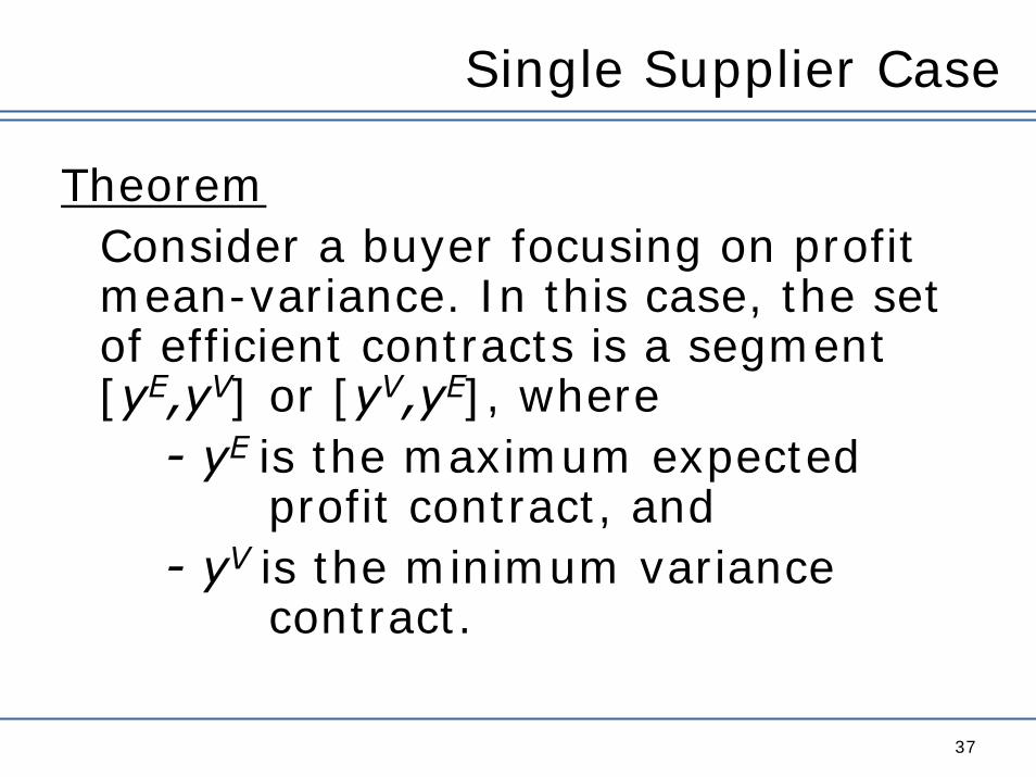
Single Supplier Case
37
TheoremConsider a buyer focusing on profit mean-variance. In this case, the set of efficient contracts is a segment [yE,yV] or [yV,yE], where
- yE is the maximum expected profit contract, and
- yV is the minimum variance contract.
Multiple Suppliers
39
TheoremConsider a buyer maximizing the objective
U=E[Π] – λ Var[Π]Then, the upper-level sets of U are connected and there is a unique local maximum y*. This portfolio is the global maximizer of the objective.
Outline
40
Portfolio contracts modelingTwo problems
Optimal replenishment policiesOptimal contract purchasing
Mean-Variance TradeoffSuppliers Competition
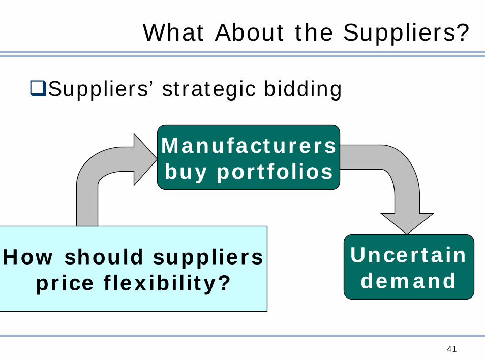
What About the Suppliers?
41
Suppliers’ strategic bidding
Manufacturersbuy portfolios
Uncertaindemand
How should suppliersprice flexibility?
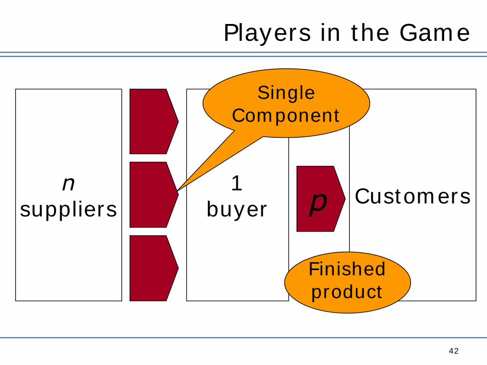
Players in the Game
42
nsuppliers
1buyer Customersp
Finishedproduct
SingleComponent
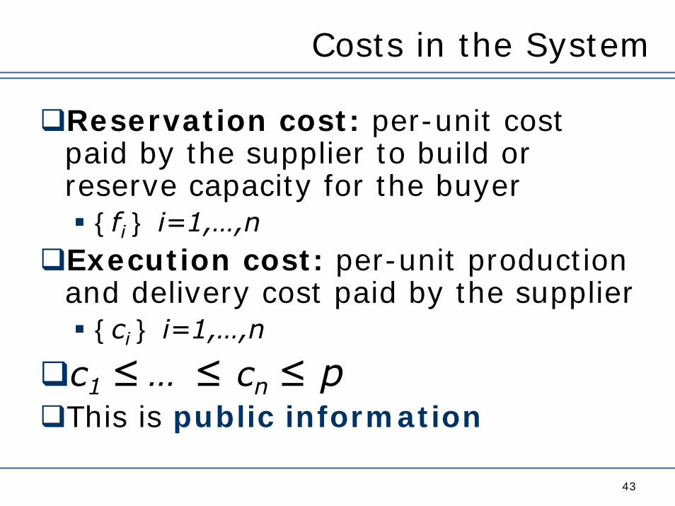
Costs in the System
43
Reservation cost: per-unit cost paid by the supplier to build or reserve capacity for the buyer
{fi } i=1,…,nExecution cost: per-unit production and delivery cost paid by the supplier
{ci } i=1,…,n
c1 ≤… ≤ cn≤ pThis is public information
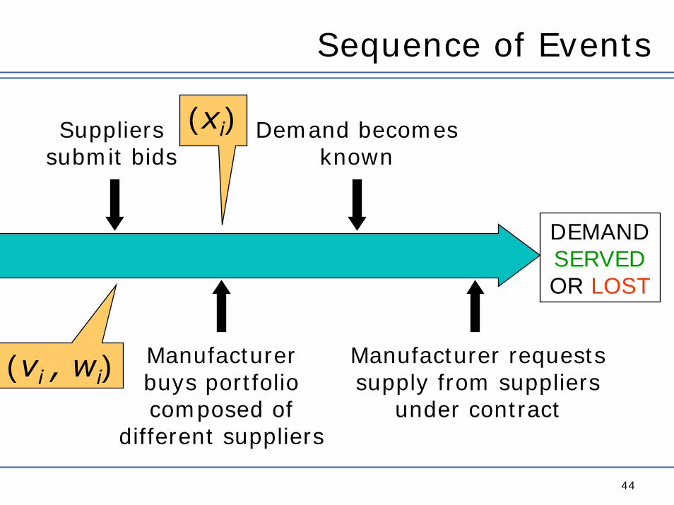
Sequence of Events
44
Suppliers submit bids
Manufacturer buys portfolio composed of
different suppliers
Demand becomes known
(xi)
DEMAND SERVEDOR LOST
Manufacturer requests supply from suppliers
under contract
(vi , wi)
45
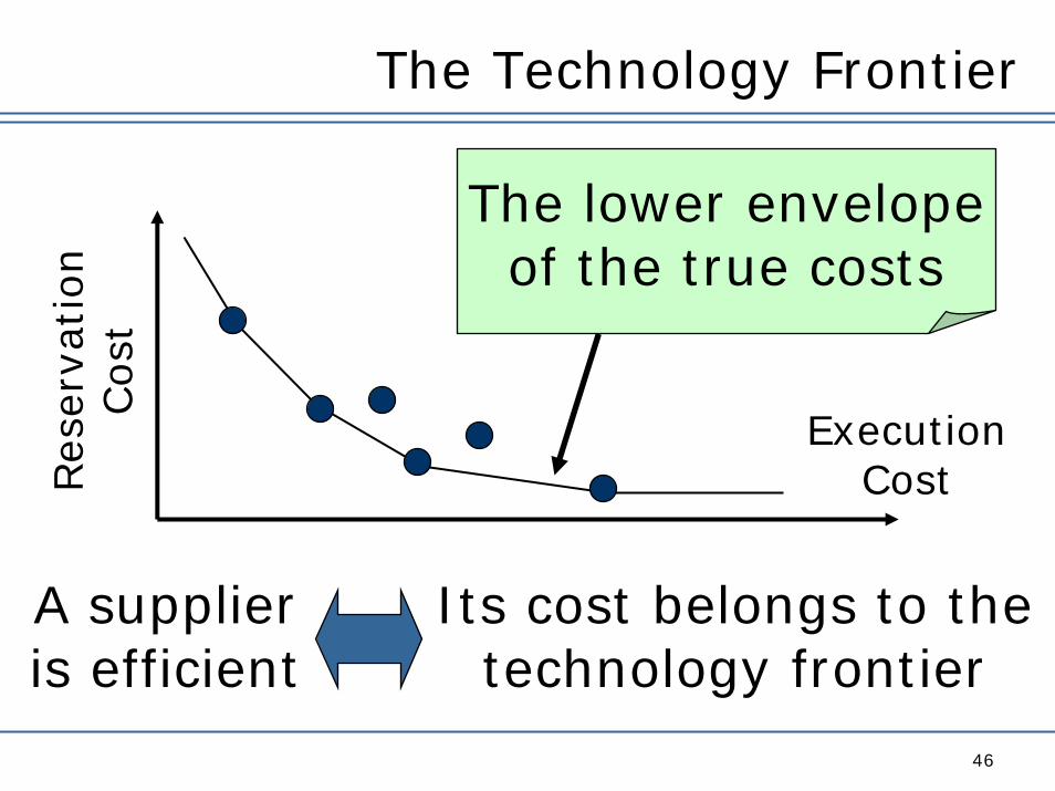
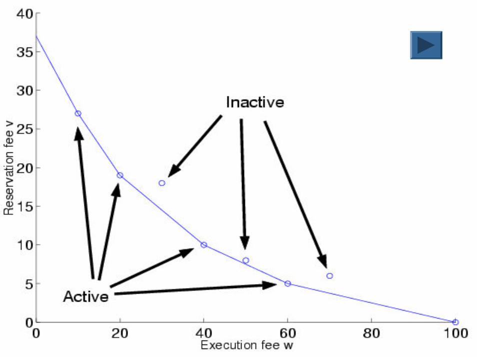
The Technology Frontier
46
A supplieris efficient
Its cost belongs to thetechnology frontier
ExecutionCost
The lower envelopeof the true costs
Res
erva
tion
Cost
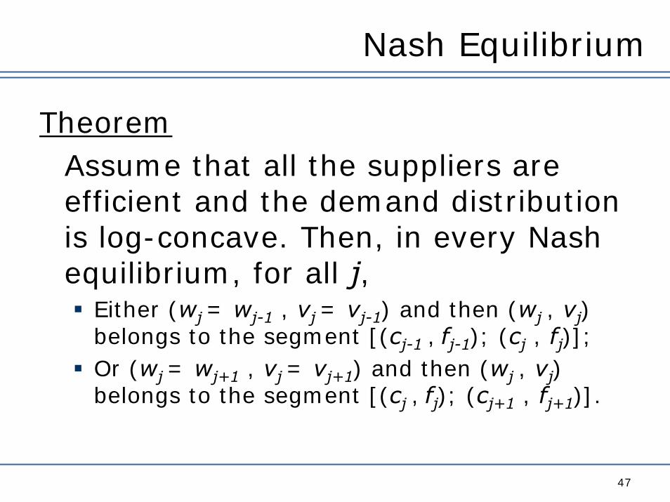
Nash Equilibrium
47
TheoremAssume that all the suppliers are efficient and the demand distribution is log-concave. Then, in every Nash equilibrium, for all j,
Either (wj = wj-1 , vj = vj-1) and then (wj , vj) belongs to the segment [(cj-1 , fj-1); (cj , fj)];Or (wj = wj+1 , vj = vj+1) and then (wj , vj) belongs to the segment [(cj , fj); (cj+1 , fj+1)].
48
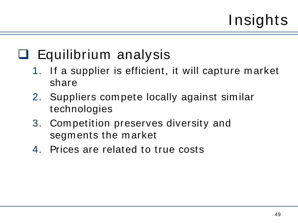
Insights
49
Equilibrium analysis1. If a supplier is efficient, it will capture market
share2. Suppliers compete locally against similar
technologies3. Competition preserves diversity and
segments the market4. Prices are related to true costs
Comparison With the Bertrand Model
50
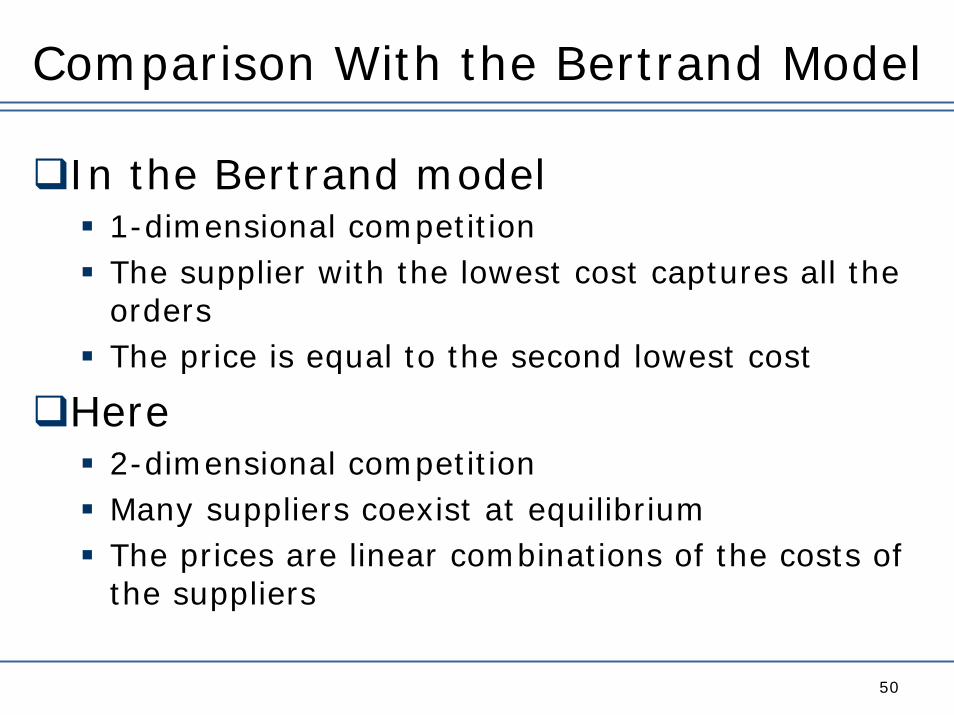
In the Bertrand model1-dimensional competitionThe supplier with the lowest cost captures all the ordersThe price is equal to the second lowest cost
Here2-dimensional competitionMany suppliers coexist at equilibriumThe prices are linear combinations of the costs of the suppliers
52
Supply Chain Profit Bounds
53
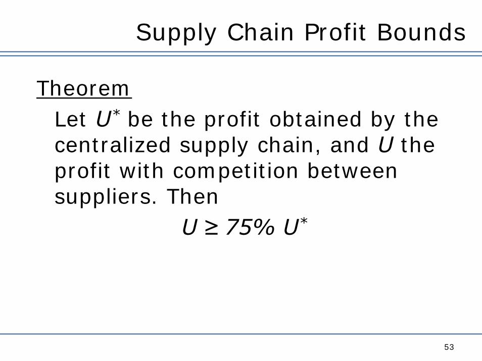
TheoremLet U* be the profit obtained by the centralized supply chain, and U the profit with competition between suppliers. Then
U≥ 75% U*
Outline
54
Literature Review
Portfolio Contracts
Risk-Averse Inventory Models
Conclusion
Risk Measures
55
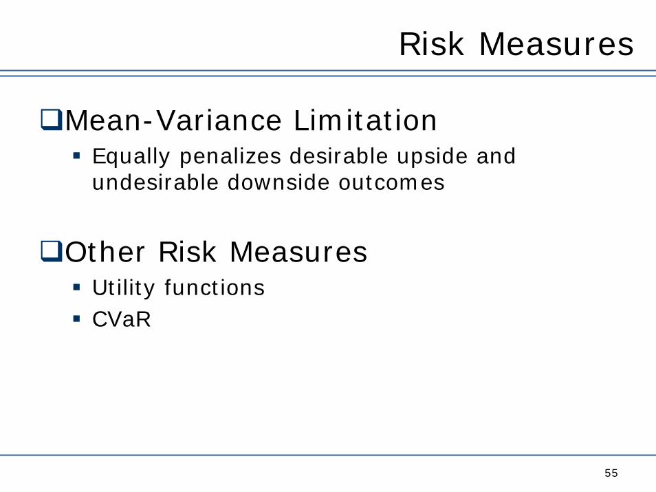
Mean-Variance LimitationEqually penalizes desirable upside and undesirable downside outcomes
Other Risk MeasuresUtility functionsCVaR
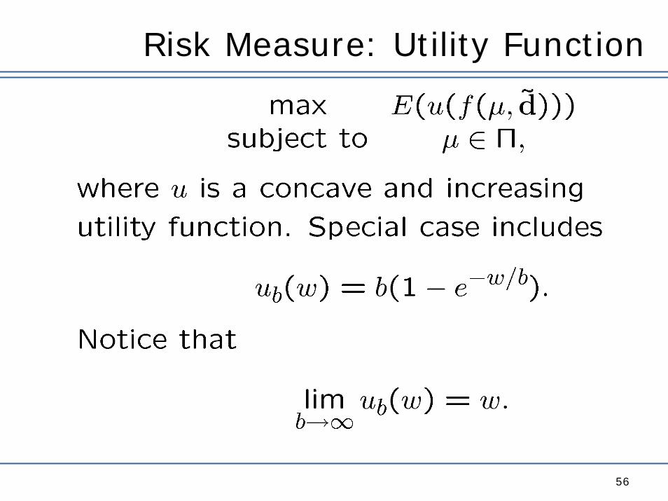
Risk Measure: Utility Function
56
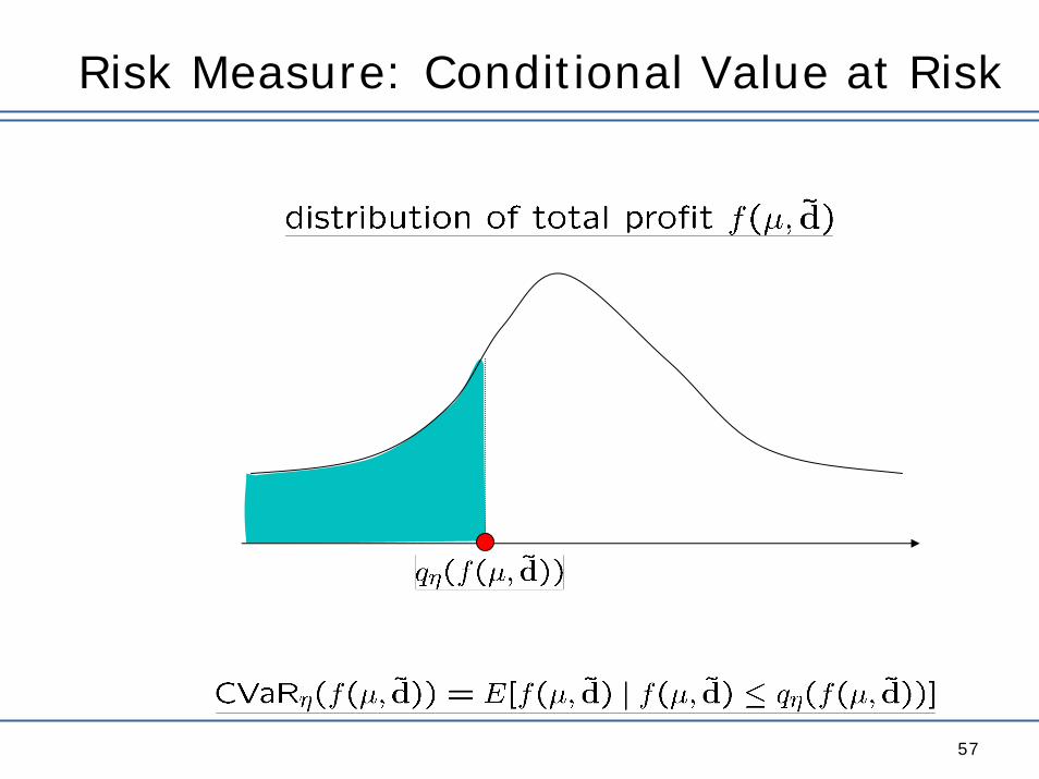
Risk Measure: Conditional Value at Risk
57
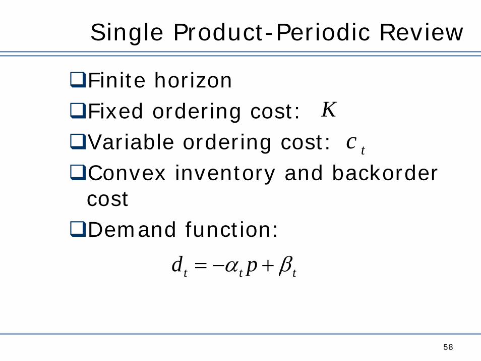
Single Product-Periodic Review
58
Finite horizonFixed ordering cost: Variable ordering cost: Convex inventory and backorder cost Demand function:
tcK
ttt pd βα +−=
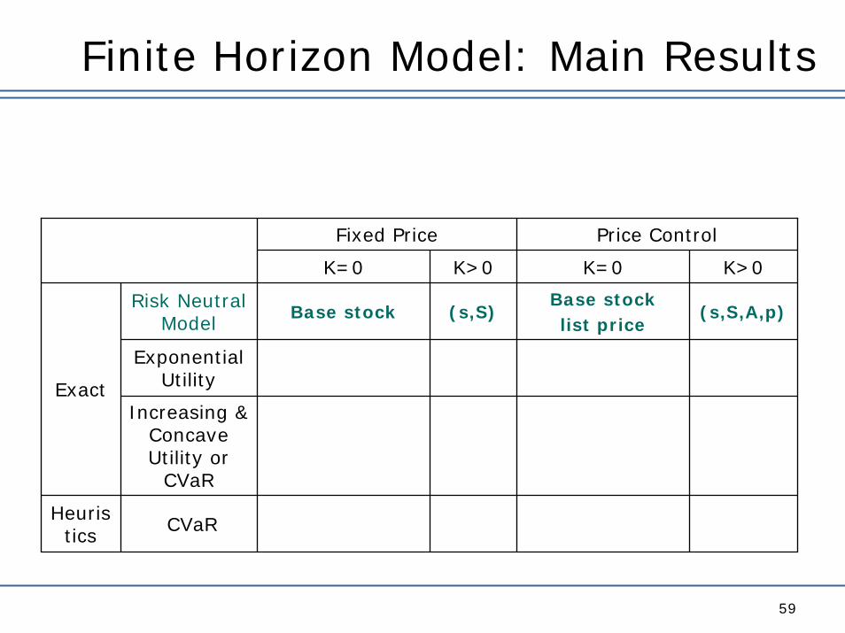
Finite Horizon Model: Main Results
59
Fixed Price Price Control
K=0 K>0 K=0 K>0
Risk NeutralModel
Base stock (s,S)Base stock list price
(s,S,A,p)
Exponential Utility
Increasing & Concave Utility or
CVaR
Heuristics CVaR
Exact

K-Concavity
60
K
s S
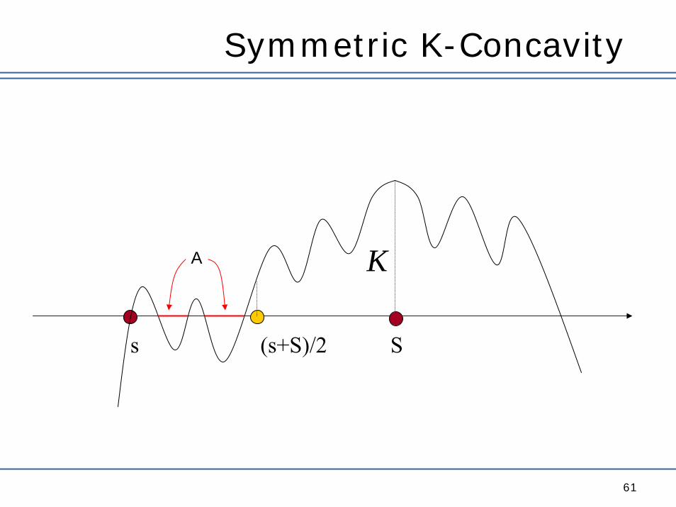
Symmetric K-Concavity
61
KA
s S(s+S)/2

Finite Horizon Model: Main Results
62
Fixed Price Price Control
K=0 K>0 K=0 K>0
Risk NeutralModel
Base stock (s,S)Base stock list price
(s,S,A,p)
Exponential Utility
Increasing & Concave Utility or
CVaR
Heuristics CVaR
Exact
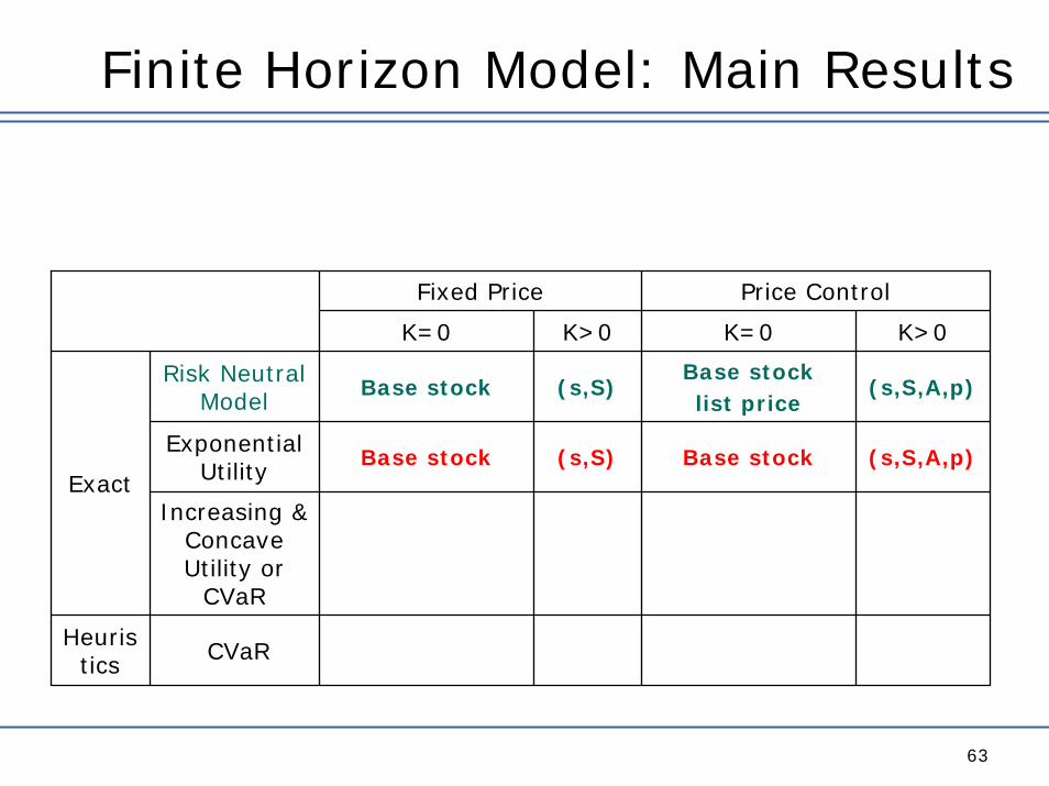
Finite Horizon Model: Main Results
63
Fixed Price Price Control
K=0 K>0 K=0 K>0
Risk NeutralModel
Base stock (s,S)Base stock list price
(s,S,A,p)
Exponential Utility
Base stock (s,S) Base stock (s,S,A,p)
Increasing & Concave Utility or
CVaR
Heuristics CVaR
Exact
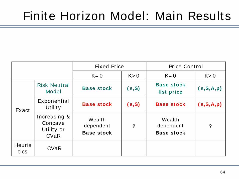
Finite Horizon Model: Main Results
64
Fixed Price Price Control
K=0 K>0 K=0 K>0
Risk NeutralModel
Base stock (s,S)Base stock list price
(s,S,A,p)
Exponential Utility
Base stock (s,S) Base stock (s,S,A,p)
Increasing & Concave Utility or
CVaR
Wealth dependent
Base stock?
Wealth dependent
Base stock?
Heuristics CVaR
Exact
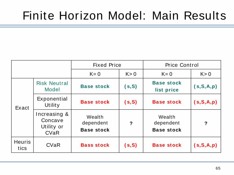
Finite Horizon Model: Main Results
65
Fixed Price Price Control
K=0 K>0 K=0 K>0
Risk NeutralModel
Base stock (s,S)Base stock list price
(s,S,A,p)
Exponential Utility
Base stock (s,S) Base stock (s,S,A,p)
Increasing & Concave Utility or
CVaR
Wealth dependent
Base stock?
Wealth dependent
Base stock?
Heuristics CVaR Bass stock (s,S) Base stock (s,S,A,p)
Exact
Extensions
66
Risk Averse Infinite Horizon Models
The Stochastic Cash Balance Problem
Models with Capacity Constraints

Questions
67
Extensions
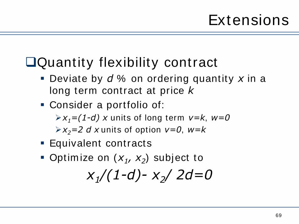
69
Quantity flexibility contractDeviate by d % on ordering quantity x in a long term contract at price kConsider a portfolio of:
x1=(1-d) x units of long term v=k, w=0x2=2 d x units of option v=0, w=k
Equivalent contractsOptimize on (x1, x2) subject to
x1/(1-d)- x2/ 2d=0
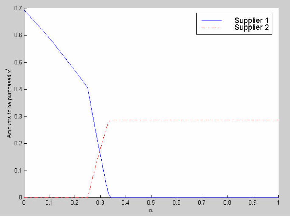
Extensions
70
Disruption managementSupplier 1 cheaper but disrupted with probability α (e.g. in Malaysia)Supplier 2 more expensive but secure (e.g. in Mexico)Trade-off here
Not flexibilityBut “credit risk” management
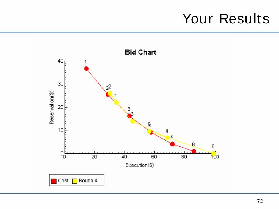
Your Results
72
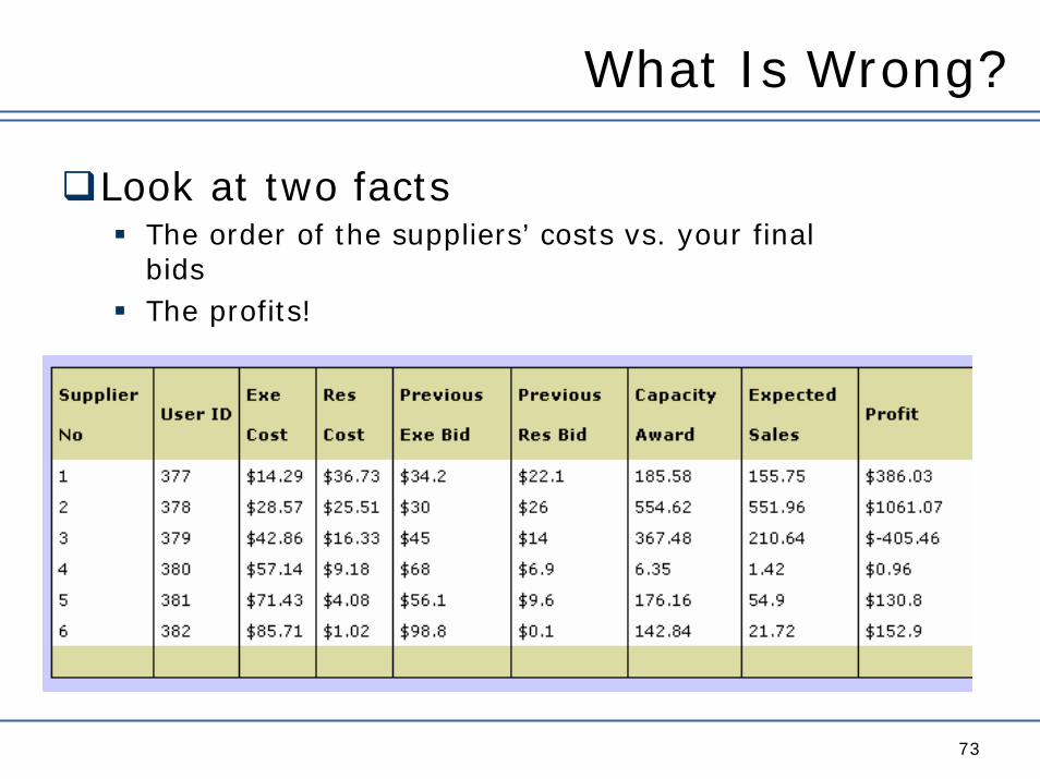
What Is Wrong?
73
Look at two factsThe order of the suppliers’ costs vs. your final bidsThe profits!
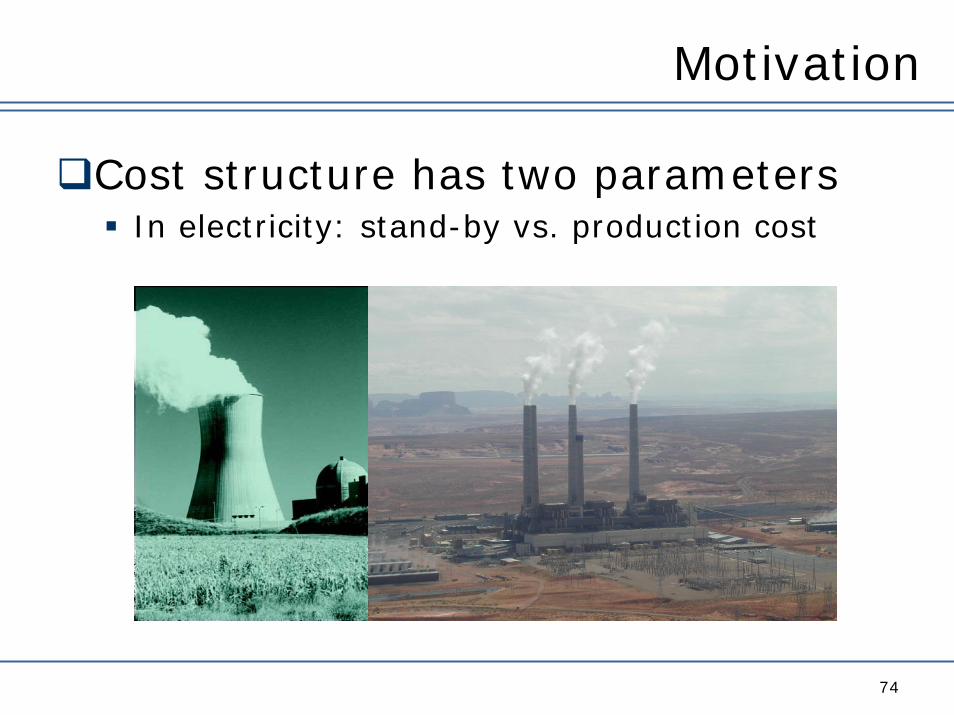
Motivation
74
Cost structure has two parametersIn electricity: stand-by vs. production cost
Example with 3 players
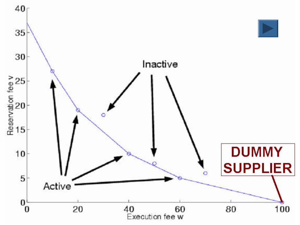
76
3 suppliersthe dummy supplier
( w=p, v=0 )
Possible outcomesCluster of 1 and 2; 3 bids with dummyCluster of 1,2 and 3: at ( w = c2 , v = f2 )
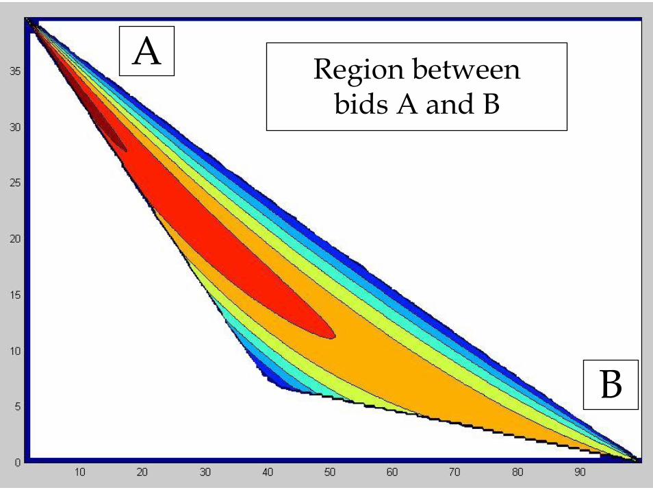
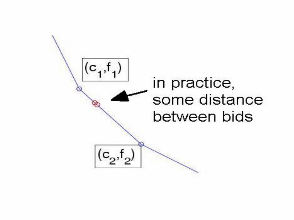
78
Region betweenbids A and B
A
B
Equilibrium Convention
79
Rationing rule: if 2 suppliers bid the same parameters (w, v)
The buyer reserves capacity and requests deliveries to both suppliers as if they were one single companyThe suppliers must share the allocations through bargainingThey cooperate in equilibriumIf there is no cooperation, by changing its bid by ε, a supplier can obtain higher profits
Alternative formalization using ε-Nash equilibrium