Unsupervised Risk Estimation with only Structural...

Unsupervised Risk Estimation with only Structural Assumptions

Jacob Steinhardt [email protected] Liang [email protected]

Stanford University, 353 Serra Mall, Stanford, CA 94305

AbstractGiven a model θ and unlabeled samples from adistribution p∗, we show how to estimate the la-beled risk of θ while only making structural (i.e.,conditional independence) assumptions about p∗.This lets us estimate a model’s test error on distri-butions very different than its training distribution,thus performing unsupervised domain adaptationeven without assuming the true predictor remainsconstant (covariate shift). Furthermore, we canperform discriminative semi-supervised learning,even under model mis-specification. Our techni-cal tool is the method of moments, which allowsus to exploit conditional independencies withoutrelying on a specific parametric model. Finally,we introduce a new theoretical framework forgrappling with the non-identifiability of the classidentities fundamental to unsupervised learning.

1. IntroductionWe study the problem of unsupervised risk estimation —that is, given a loss function L(θ;x, y), and a test distribu-tion p∗(x, y), estimate the risk R(θ)

def= Ex,y∼p∗ [L(θ;x, y)]

given access only to m unlabeled examples x(1:m) i.i.d.∼p∗(x). Can we do this without making strong parametricassumptions about p∗? Although perhaps daunting at firstglance, previous work has successfully made progress byonly requiring parametric assumptions on the losses; for in-stance, Balasubramanian et al. (2011) assume Gaussianityof model scores, while a line of work starting with Dawid& Skene (1979) assume multiple classifiers with known de-pendency structure, which specifies a complete generativedistribution for the 0/1-loss (Zhang et al., 2014; Platanios,2015; Jaffe et al., 2015).

In this work, we show that modeling the losses is unneces-sary, and that we can in fact recover the risk for multiclassclassification while only making conditional independence

This is a preliminary manuscript, last updated February 2016.Please send any errors or comments to the first author.

label:

inputs:

L(x, y) = A(x)

y

x1 x2 x3

−f1(x1, y) −f2(x2, y) −f3(x3, y)

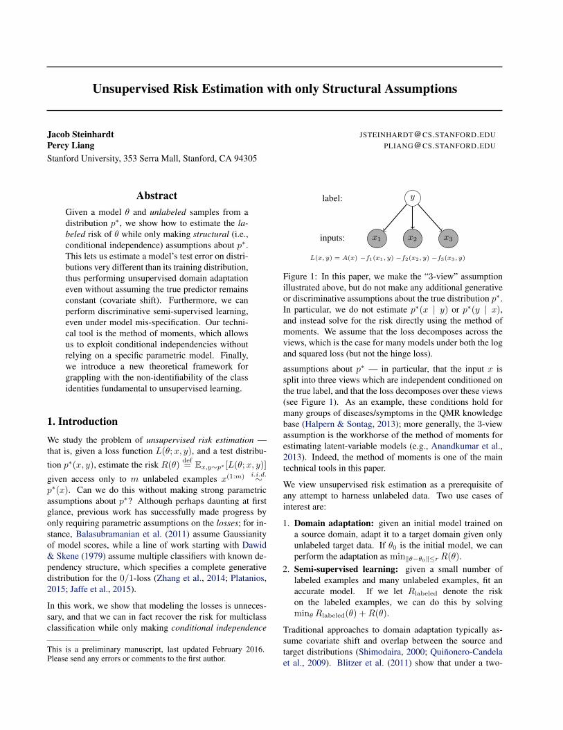
Figure 1: In this paper, we make the “3-view” assumptionillustrated above, but do not make any additional generativeor discriminative assumptions about the true distribution p∗.In particular, we do not estimate p∗(x | y) or p∗(y | x),and instead solve for the risk directly using the method ofmoments. We assume that the loss decomposes across theviews, which is the case for many models under both the logand squared loss (but not the hinge loss).

assumptions about p∗ — in particular, that the input x issplit into three views which are independent conditioned onthe true label, and that the loss decomposes over these views(see Figure 1). As an example, these conditions hold formany groups of diseases/symptoms in the QMR knowledgebase (Halpern & Sontag, 2013); more generally, the 3-viewassumption is the workhorse of the method of moments forestimating latent-variable models (e.g., Anandkumar et al.,2013). Indeed, the method of moments is one of the maintechnical tools in this paper.

We view unsupervised risk estimation as a prerequisite ofany attempt to harness unlabeled data. Two use cases ofinterest are:

1. Domain adaptation: given an initial model trained ona source domain, adapt it to a target domain given onlyunlabeled target data. If θ0 is the initial model, we canperform the adaptation as min‖θ−θ0‖≤r R(θ).

2. Semi-supervised learning: given a small number oflabeled examples and many unlabeled examples, fit anaccurate model. If we let Rlabeled denote the riskon the labeled examples, we can do this by solvingminθ Rlabeled(θ) +R(θ).

Traditional approaches to domain adaptation typically as-sume covariate shift and overlap between the source andtarget distributions (Shimodaira, 2000; Quinonero-Candelaet al., 2009). Blitzer et al. (2011) show that under a two-


view assumption, source-target overlap is unnecessary. Ourresults show that with three independent views, even the co-variate shift assumption can be done away with.

One approach to semi-supervised learning is to build a gen-erative model over x and y, and include the marginal like-lihood on the unlabeled examples as part of the cost func-tion during learning. However, a wide body of empiricalevidence shows that, when the generative model is mis-specified, the unlabeled examples can actually degrade per-formance (Merialdo, 1994; Cozman & Cohen, 2006; Liang& Klein, 2008; Li & Zhou, 2015). Because of this, two-view assumptions have been used as an alternative to thegenerative approaches (Blum & Mitchell, 1998; Ando &Zhang, 2007; Kakade & Foster, 2007; Balcan & Blum,2010). These methods all assume some form of low noise orlow regret, as do other methods such as transductive SVMs(Joachims, 1999). Our results imply that, with three inde-pendent views, such assumptions are unnecessary.

By focusing on the central problem of risk estimation, ourwork connects multi-view learning approaches for domainadaptation and semi-supervised learning, and extends themto remove covariate shift and low-noise assumptions. Ourwork does not strictly generalize the work above, as for in-stance Kakade & Foster (2007) and Blitzer et al. (2011) as-sume low regret but not independence, and consider regres-sion rather than classification.

Finally, we treat a fundamental identifiability issue — thatthe class identities are only recoverable up to permutationin any unsupervised setting. Previous work required strongassumptions to circumvent this issue (e.g. that the classprobabilities are distinct and known (Balasubramanian et al.,2011) or that the classifiers are correct on average (Jaffeet al., 2015)). We instead show that, as long as the modelslightly outperforms random guessing, the class identitiesare correct with high probability. We do this by formulat-ing a robust Bayesian hypothesis test whose performanceis justified via a novel notion of identifiability index, us-ing classical tools such as metric entropy (Kolmogorov &Tikhomirov, 1959; Lorentz, 1966), fractional covering num-bers (Lovasz, 1975), and Lipschitz concentration of Gaus-sians (Tsirelson et al., 1976).

While previous work has used multi-view assumptions toestimate the 0/1-risk, our setting is quite different, as the as-sumptions in e.g. Zhang et al. (2014) or Jaffe et al. (2015)yield a fully-specified family for the distribution of 0/1-losses, and they proceed by estimating this distribution. Incontrast, we directly estimate the risk without needing to es-timate the underlying distribution of losses.

Our main technical results are:

• Risk Estimation: we estimate the risk R(θ) to error εgiven a number of unlabeled samples that depends on ε

and the number of classes k, but not on the dimension dof θ (Theorem 2.2).• Learning: given poly(k) · d log(d)

ε2 unlabeled samples,we learn the optimal parameters θ up to error ε (Corol-lary 3.2).• Identifiability: We develop a robust Bayesian hypothesis

test (Algorithm 2), and show that if the estimated risk is atleast slightly better than random guessing, then we havevery likely identified the true classes.

2. Framework and Estimation AlgorithmWe will focus on multiclass classification; we assume an un-known true distribution p∗(x, y) over X × Y , where Y =1, . . . , k, and are given unlabeled samples x(1), . . . , x(m)

drawn independently from p∗(x). Given parameters θ ∈ Rdand a loss function L(θ;x, y), our goal is to estimate the riskof θ on p∗:

R(θ)def= Ex,y∼p∗ [L(θ;x, y)]. (1)

Throughout, we will make the 3-view assumption:Assumption 2.1 (3-view). Under p∗, x can be split intox1, x2, x3, which are conditionally independent given y (seeFigure 1). Moreover, the loss decomposes additively acrossviews: L(θ;x, y) = A(θ;x) −

∑3v=1 fv(θ;xv, y), for some

functions A and fv .

Often L will be the log loss for a model pθ(y | x) ∝exp(θ>

∑3v=1 φv(xv, y)), in which case fv(θ;xv, y) =

θ>φv(xv, y) and A(θ;x) is the log partition function.

Note that Assumption 2.1 is not enough to recover R, be-cause permuting the classes 1, . . . , k will preserve p∗(x)(as well as the conditional independence) but will changethe risk R. However, it turns out that this is the only thingthat is unknown; in particular, define the optimistic risk Ras the minimum risk over all permutations of the classes:

R(θ)def= min

σ∈Sym(k)Ex,y∼p∗ [L(θ;x, σ(y))], (2)

where Sym(k) is the group of permutations on 1, . . . , k.We will show that R can be recovered, as Theorem 2.2 indi-cates below. The key insight is that, even without estimatingp∗(y | x), we can express R(θ) in terms of certain momentsof p∗, which are obtained as the solution to a system of cu-bic equations (corresponding to 3rd-order moments) derivedfrom Assumption 2.1.

We start by expanding the definition of R:

R(θ) = A(θ)−Rlinear(θ), where

A(θ)def= Ex∼p∗ [A(θ;x)],

Rlinear(θ)def=

k∑j=1

p∗(y = j)

3∑v=1

E[fv(θ;xv, j) | y = j].


The first term A can be estimated from only unlabeled data,while the second term Rlinear can be expressed in terms ofthe conditional expectations µj,v = E[fv | y = j], moreformally defined as (suppressing the dependence on θ):

µj,vdef= E[hv(x) | y = j], where

hv(x)def= [fv(θ;xv, 1) · · · fv(θ;xv, k)]

>. (3)

Thus hv(x) is the vector of model scores, while µj,v is themean score vector across class j. If we let πj = p∗(y = j)

for convenience, then Rlinear(θ) =∑kj=1 πj

∑3v=1(µj,v)j .

This is useful as it implies that, to estimate R, we need onlyestimate π and µ.

From here, we follow the technical machinery behind thespectral method of moments (e.g., Anandkumar et al., 2012),which we explain for completeness. The conditional inde-pendence of the xv means that conditioned on y = j, thesecond- and third-order moments of h are products of thefirst-order moments µj,v . By marginalizing over y, we ob-tain the following equations, where⊗ is the Kronecker prod-uct (also called outer product or tensor product):

E[hv(x)] =

k∑j=1

πjµj,v

E[hv(x)⊗hv′(x)] =

k∑j=1

πjµj,v ⊗ µj,v′ for v 6= v′

E[h1(x)⊗h2(x)⊗h3(x)] =

k∑j=1

πjµj,1 ⊗ µj,2 ⊗ µj,3 (4)

Note that the left-hand-side of each equation can be esti-mated from unlabeled data. There are more independentequations than unknowns in (4) for any k ≥ 2; in particular,Anandkumar et al. (2012) show (see Theorem 7 therein) thatwe can recover π and µ up to permutation: that is, there issome permutation σ ∈ Sym(k) such that p∗(y = j) ≈ πσ(j)

and E[hv(x) | y = j] ≈ µσ(j),v .

Implications. Once we have π and µ, we can plug back intoR. If we had σ, we could plug in exactly:

R(θ) = A(θ)−k∑j=1

p∗(y = j)

3∑v=1

E[fv(θ;xv, j) | y = j]

≈ A(θ)−k∑j=1

πσ(j)

3∑v=1

(µσ(j),v)j

Since we don’t know σ, we can instead take the minimumover all σ, which yields R. This minimization is an instanceof maximum weight bipartite matching, and can be solvedin O

(k3)

time; see Section A for details.

Putting all of the above ideas together, we obtain Theo-rem 2.2, which gives a sample complexity bound for es-timating R that depends on the number of classes k, the

minimum class probability πmin, the second moment of theloss τ , and the minimum singular value σk(Mv), whereMv

def= [µ1,v · · · µk,v]. More formally:

Theorem 2.2. Suppose Assumption 2.1 holds. Then, we canestimate R(θ) to accuracy ε with probability 1 − δ for any0 < ε, δ < 1 using

m = poly(k, π−1

min, λ−1, τ

)· log(2/δ)

ε2samples, where

πmindef=

kminj=1

πj ,

τdef= max

(maxj,v

√E[‖hv‖22| y = j],

√E[A2]

), and

λdef=

3minv=1

σk(Mv). (5)

For a full proof, see Section B. In summary, Assumption 2.1yields a set of moment equations (4) that, when solved, al-low us to estimate the optimistic risk R(θ).

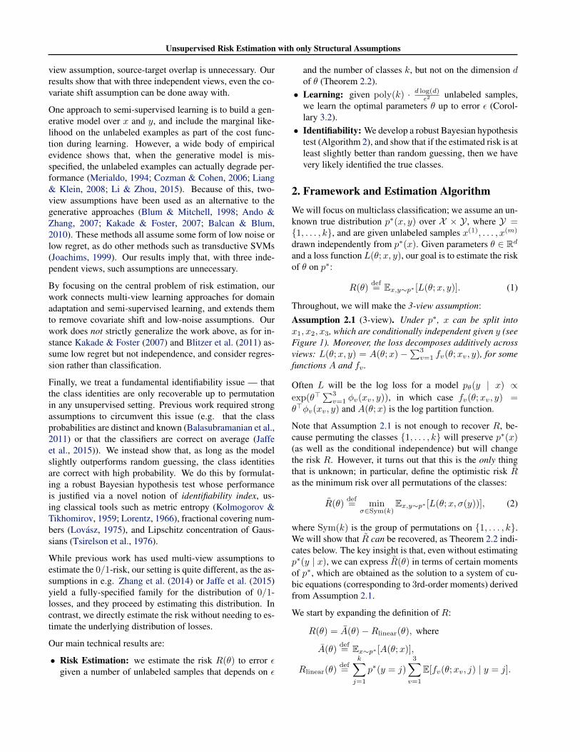
3. From Estimation to LearningIn the previous section, we saw how to estimate the riskR(θ) up to permutation of the labels. We now turn to theproblem of learning, i.e., minimizing over θ ∈ Rd. We willfirst show how to compute the gradient ∇θR, and next at-tend to the difference between minimizing R(θ) and mini-mizing R(θ). For the latter, we assume that we have at leastan initial point θ0 in a certain “good” region Θ0, often ob-tainable by training on a related task or from a small amountof supervised data. To elaborate on this, we provide somegeometric intuition about R and R.

Let Rσ(θ) be the risk when the labels are permuted byσ: Rσ(θ)

def= Ex,y∼p∗ [L(θ;x, σ(y))]. Then R = Rid,

where id is the identity permutation, while R is theminimum of the functions Rσ . This is illustrated below:

θ

L

“good” region Θ0

gap

Rσ1

R

Rσ2

R

We define Θ0 to be the region where R(θ) = R(θ), orequivalently where minσ 6=idR

σ(θ) − Rid(θ) ≥ 0. Definegap(θ) to be the difference between the smallest andsecond-smallest values (over σ) of Rσ(θ); then gap(θ) = 0


at the boundary of Θ0. The gap measures how easy it is tomix up two of the curves Rσ in the presence of noise.

Computing the gradient. To compute ∇θR, thestraightforward approach is (recalling R(θ) = A(θ) −∑3v=1 E[fv(θ;x, y)]) to take the vectors ∇θfv and compute

their expectations similarly to Theorem 2.2. However, equa-tion (4) would then involve a kd × kd × kd tensor, whichis prohibitive even for e.g. k = 2, d = 104. Instead, wetake an approach inspired by Nesterov & Spokoiny (2011),which is to compute the directional derivative u>∇θfv (re-quiring only a k × k × k tensor) and from several such uapproximate the full gradient.

In particular, we take u ∈ Rd and replace fv in equa-tion (4) with u>∇θfv , thus estimating u>∇θRlinear =∑3v=1 Ex,y[u>∇θfv] from only poly(k) samples. By sam-

pling many such u, we can estimate the full gradient as∑3v=1 Eu,x,y[uu>∇θfv(x, y)], assuming E[uu>] = Id×d.

This still does not quite work, because we only obtain eachu>∇θfv up to a permutation σu, which will be different fordifferent u. We remedy this by simultaneously estimating fvand u>∇θfv; since fv is the same each time, we can use it toundo the permutations σu, allowing us to correctly averageacross u. The full procedure is given as Algorithm 1, andrequires log(d/ε) times as many samples as in Theorem 2.2.In particular (see Section C for proof):

Theorem 3.1. Suppose that Algorithm 1 is run with m =

poly(k, π−1

min, λ−1, τ

)· log(d/εδ)

ε2 samples as input at a pointθ0, and that ε < min(1, gap(θ0)). Then with probability1− δ, the output of Algorithm 1 is a vector g satisfying

∥∥∥g −∇Rlinear(θ0)∥∥∥

2≤ εB, (6)

where B2 = max3v=1 E[maxkj=1‖∇θfv(θ0;x, j)‖22] mea-

sures the squared `2-norm of the gradient.

Note that Algorithm 1 can likely be improved substantiallyby replacing the random projections with fast low-rank pro-jections (Halko et al., 2011), which would allow efficientdirect computation of the full gradient.

Linear models. When the fv are linear in θ — e.g. for mul-ticlass logistic regression — evaluating the gradient once issufficient for all iterations of learning. The reason is thatR(θ) is then equal to A(θ)− θ>∇θRlinear(θ0), for any vec-tor θ0 ∈ Θ0. As long as we regularize θ by constraining‖θ‖2≤ ρ, approximating ∇Rlinear with g will still yield anear-optimal θ. In particular (again see Section C):

Corollary 3.2. Suppose that fv(θ;xv, y) = θ>φv(xv, y),where ‖φv(xv, j)‖2≤ B for all v, xv , j and that A(θ;x) isB-Lipschitz in θ. Also suppose that we run Algorithm 1 ata point θ0 ∈ Θ0 to obtain g. Then, if ε and m satisfy the

Algorithm 1 Algorithm for computing the gradient of R.Input: initial parameters θ0 ∈ Rd, samples x(1:m) ∼ p∗.Define hv(x, u) ∈ R2k as

hv(x, u) = [fv(θ0;xv, j) u>∇θfv(θ0;xv, j)/B]kj=1

for t = 1 to T = 75d log(2d/δ)ε2 do

Sample ut uniformly from ±1d.Using x(1:m), estimate the moments

E[hv(x, ut)],E[hv1(x, ut)⊗ hv2(x, ut)], andE[h1(x, ut)⊗ h2(x, ut)⊗ h3(x, ut)].

Use tensor decomposition to compute πj,t ≈ πj , µj,t ≈∑v µj,v , and gj,t ≈

∑v E[u>t ∇θfv(θ0;xv, j) | j].

Permute the rows of µj,t (and simultaneously gj,t) suchthat

∑j πj,t(µj,t)j is maximized.

end forOutput g = 1

T

∑Tt=1 ut

∑kj=1 πj,tgj,t.

conditions in Theorem 3.1, and we let

θ = arg min‖θ‖2≤ρ

1

m

m∑i=1

A(θ;x(i))− θ>g, (7)

then R(θ) ≤ min‖θ‖2≤ρR(θ) + 2εBρ with probability 1 −2δ.

If e.g. ‖θ‖2= ‖φ‖∞= 1, then we will have ρ = 1 andB ≤

√d, whence we need ε 1/

√d to obtain good bounds

on R(θ); Corollary 3.2 then implies a sample complexity ofpoly

(k, π−1

min, λ−1, τ

)· d log(d/εδ).

A general criterion. If the fv are non-linear, we likely needto evaluate R at more than one point, and there is no guar-antee that R(θ) = R(θ) once we move away from θ0. Tohelp address this, we provide a criterion which certifies that,given an initial point θ0 ∈ Θ0, a new point θ will also lie inΘ0:

Lemma 3.3. Suppose θ0 ∈ Θ0, and θ satisfies

Ex∼p∗[

kmaxj=1|f(θ;x, j)− f(θ0;x, j)|

]<

1

2(gap(θ0) + gap(θ)) ,

(8)where f =

∑3v=1 fv . Then, θ ∈ Θ0 as well.

See Section D for a proof. The idea is that the left handside of (8) bounds the amount that any of the Rσ (or moreprecisely, Rσ − A) can move. Note that the left-hand-sideof (8) can be estimated from unlabeled data.

We can use Lemma 3.3 to modify any optimization proce-dure: given any proposed next point θt+1, backtrack in thedirection of the current point θt until (8) holds, and thencontinue the optimization. Note however that if (8) is overlyconservative then we may not reach the optimum.


q1

q2

q3

q4

q5

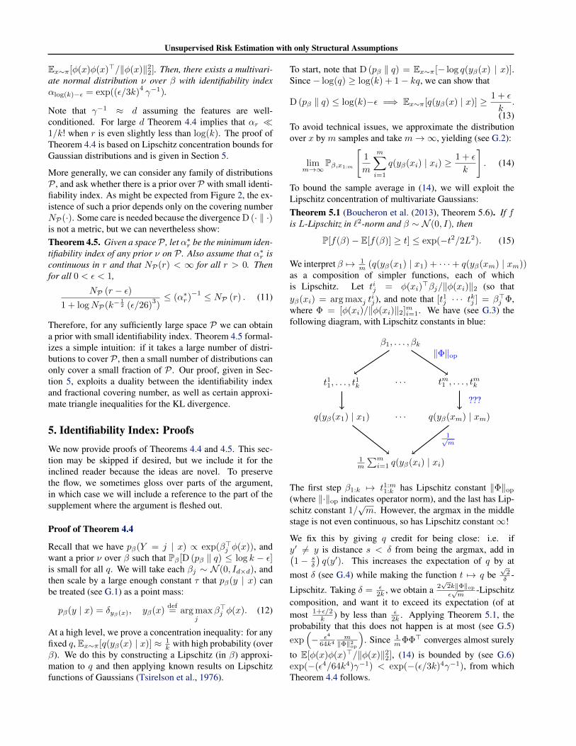
Figure 2: Illustration of Definition 4.1. Each ball is a setBr(q) = p | D (p ‖ q) ≤ r. If no single ball has largeprobability mass under ν, then no small number of distribu-tions q1, . . . , qM can fit a random distribution from ν well.

4. Identifiability IndexIn Section 2, we showed how to identify the riskR up to per-mutation of the classes (thus instead obtaining the optimisticrisk R). We now study more carefully how this optimismcan affect our estimate of the risk. This will help us avoidfalse negatives where R is small but R is large; at a highlevel, we will see that if R is better than random guessing,then R = R with high probability.

Intuitively, a generic “bad” distribution is simply not veryrelated to the model, and so none of its permutation will be,either. To formalize what is meant by generic, we adopt arobust Bayesian perspective: we define a prior ν over pos-sible input distributions p∗, and design a test with low falsenegative rate under the prior, where the test is (nearly) inde-pendent of the choice of ν. In the following, we restrict tothe log loss, as the proofs are already hard for this case.

Identifiability index. If we think of the k! permutations ofthe classes as simply k! candidate models, then the ques-tion becomes: how high can we make the probability thatat least one of the models looks good by chance? We adopta Bayesian approach and suppose that the true distributionp∗(y | x) is drawn from a prior ν. For a given q(y | x), wecan consider the ball of possible p∗ that are fit well by q; ifall such balls have low mass under ν, then it is impossible tofit p∗ well by chance (this is illustrated in Figure 2).

Formally, we take the ball Br(q)def= p | D (p ‖ q) ≤ r;

here the divergence D (p ‖ q) is the average KL divergence

D (p ‖ q) def= Ex∼π[KL (p(· | x) ‖ q(· | x))], (9)

where π(x) is the distribution over x. We then define theidentifiability index of ν to be the most mass that can becovered by a single such ball:

Definition 4.1 (Identifiability index). For a given r,the identifiability index αr for a prior ν is defined assupq ν(Br(q)).

In particular, if αr 1k! , then it is unlikely that any of

the k! permutations of a model pθ would have low risk bychance. We will see below (Theorem 4.4) that αr is oftenexp(−Ω(d)) for d-dimensional exponential families.

Algorithm 2 Algorithm for checking that R(θ) = R(θ).

Input: model pθ, failure probability δ, samples x(1:m).Let r0 satisfy αr0 ≤ δ

k! .Return true if R(θ) ≤ r0, else false.

In addition to the identifiability index, we also care abouthow well-separated the classes are — if they are not verywell-separated, then it is more likely that two classes havebeen mixed up. We can formalize this by looking at theminimum gap in risk from getting a single class wrong:

Definition 4.2 (Class separation). The class separation γ(θ)

of pθ is defined as γ(θ)def= minj′ 6=j(µj)j − (µj)j′ , where

µj =∑3v=1 µj,v is the mean score across class j.

Note that we cannot estimate the class separation (since itdepends on the true permutation of the µj), so we assumethat either γ(θ) > 0, or p∗ is drawn at random from ν. Wecan then check that R(θ) = R(θ) (with failure probabilityδ) by checking that R(θ) ≤ r0, where αr0 ≤ δ/k!. Thistest is depicted in Algorithm 2. The validity of this test iscertified by Proposition 4.3 (proved in Section E):

Proposition 4.3. Suppose that ν has identifiability index αr,and that ν′ induces positive class separation (γ(θ) > 0) withprobability 1. Then, if p∗ ∼ ν, with ν ∈ ν, ν′, we have thefalse negative bound

maxν∈ν,ν′

Pν [R(θ) ≤ r ∧ R(θ) 6= R(θ)] ≤ k!αr. (10)

Thus, assuming that p∗ either has positive separation or isdrawn at random from ν, Algorithm 2 has a false negativerate of at most δ. The test depends on the prior ν onlythrough the identifiability index, which we show below issmall for many priors, even when r = log(k)− ε (note thatlog(k) is the risk of uniform guessing).

Identifiability and learning. The intuition in Figure 2 alsoapplies in the learning setting, if instead of the k! permuta-tions of a fixed model we consider all models in some fam-ily Θ. We can bound the false negative rate under p∗ ∼ νin terms of the identifiability index as well as the cover-ing number of Θ (i.e., the minimum number of balls Br(q)needed to cover Θ); details are in Section F.

Computing αr. We referred to Algorithm 2 as a ro-bust Bayesian hypothesis test because the test depends onthe prior ν only through the identifiability index αr. Westrengthen the robustness argument by showing that αr issmall — typically exponentially small in the dimension.

To start, for exponential families, the identifiability index αris large under a Gaussian prior:

Theorem 4.4. Consider an exponential family defined by φ,i.e. pβ(y | x) ∝ exp(β>y φ(x)). Assume that φ(x) 6= 0almost surely, and let γ be the maximum singular value of


Ex∼π[φ(x)φ(x)>/‖φ(x)‖22]. Then, there exists a multivari-ate normal distribution ν over β with identifiability indexαlog(k)−ε = exp((ε/3k)

4γ−1).

Note that γ−1 ≈ d assuming the features are well-conditioned. For large d Theorem 4.4 implies that αr 1/k! when r is even slightly less than log(k). The proof ofTheorem 4.4 is based on Lipschitz concentration bounds forGaussian distributions and is given in Section 5.

More generally, we can consider any family of distributionsP , and ask whether there is a prior over P with small identi-fiability index. As might be expected from Figure 2, the ex-istence of such a prior depends only on the covering numberNP(·). Some care is needed because the divergence D (· ‖ ·)is not a metric, but we can nevertheless show:Theorem 4.5. Given a spaceP , letα∗r be the minimum iden-tifiability index of any prior ν on P . Also assume that α∗r iscontinuous in r and that NP(r) < ∞ for all r > 0. Thenfor all 0 < ε < 1,

NP (r − ε)1 + logNP(k−

12 (ε/26)

3)≤ (α∗r)

−1 ≤ NP (r) . (11)

Therefore, for any sufficiently large space P we can obtaina prior with small identifiability index. Theorem 4.5 formal-izes a simple intuition: if it takes a large number of distri-butions to cover P , then a small number of distributions canonly cover a small fraction of P . Our proof, given in Sec-tion 5, exploits a duality between the identifiability indexand fractional covering number, as well as certain approxi-mate triangle inequalities for the KL divergence.

5. Identifiability Index: ProofsWe now provide proofs of Theorems 4.4 and 4.5. This sec-tion may be skipped if desired, but we include it for theinclined reader because the ideas are novel. To preservethe flow, we sometimes gloss over parts of the argument,in which case we will include a reference to the part of thesupplement where the argument is fleshed out.

Proof of Theorem 4.4

Recall that we have pβ(Y = j | x) ∝ exp(β>j φ(x)), andwant a prior ν over β such that Pβ [D (pβ ‖ q) ≤ log k − ε]is small for all q. We will take each βj ∼ N (0, Id×d), andthen scale by a large enough constant τ that pβ(y | x) canbe treated (see G.1) as a point mass:

pβ(y | x) = δyβ(x), yβ(x)def= arg max

jβ>j φ(x). (12)

At a high level, we prove a concentration inequality: for anyfixed q, Ex∼π[q(yβ(x) | x)] ≈ 1

k with high probability (overβ). We do this by constructing a Lipschitz (in β) approxi-mation to q and then applying known results on Lipschitzfunctions of Gaussians (Tsirelson et al., 1976).

To start, note that D (pβ ‖ q) = Ex∼π[− log q(yβ(x) | x)].Since − log(q) ≥ log(k) + 1− kq, we can show that

D (pβ ‖ q) ≤ log(k)−ε =⇒ Ex∼π[q(yβ(x) | x)] ≥ 1 + ε

k.

(13)To avoid technical issues, we approximate the distributionover x by m samples and take m→∞, yielding (see G.2):

limm→∞

Pβ,x1:m

[1

m

m∑i=1

q(yβ(xi) | xi) ≥1 + ε

k

]. (14)

To bound the sample average in (14), we will exploit theLipschitz concentration of multivariate Gaussians:Theorem 5.1 (Boucheron et al. (2013), Theorem 5.6). If fis L-Lipschitz in `2-norm and β ∼ N (0, I), then

P[f(β)− E[f(β)] ≥ t] ≤ exp(−t2/2L2). (15)

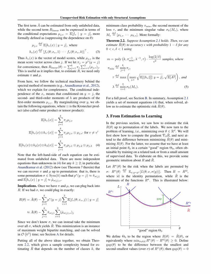
We interpret β 7→ 1m (q(yβ(x1) | x1) + · · ·+ q(yβ(xm) | xm))

as a composition of simpler functions, each of whichis Lipschitz. Let tij = φ(xi)

>βj/‖φ(xi)‖2 (so thatyβ(xi) = arg maxj t

ij), and note that [t1j · · · tkj ] = β>j Φ,

where Φ = [φ(xi)/‖φ(xi)‖2]mi=1. We have (see G.3) thefollowing diagram, with Lipschitz constants in blue:

β1, . . . , βk

t11, . . . , t1k · · · tm1 , . . . , t

mk

q(yβ(x1) | x1) · · · q(yβ(xm) | xm)

1m

∑mi=1 q(yβ(xi) | xi)

‖Φ‖op

???

1√m

The first step β1:k 7→ t1:m1:k has Lipschitz constant ‖Φ‖op

(where ‖·‖op indicates operator norm), and the last has Lip-schitz constant 1/

√m. However, the argmax in the middle

stage is not even continuous, so has Lipschitz constant∞!

We fix this by giving q credit for being close: i.e. ify′ 6= y is distance s < δ from being the argmax, add in(1− s

δ

)q(y′). This increases the expectation of q by at

most δ (see G.4) while making the function t 7→ q be√

2δ -

Lipschitz. Taking δ = ε2k , we obtain a 2

√2k‖Φ‖opε√m

-Lipschitzcomposition, and want it to exceed its expectation (of atmost 1+ε/2

k ) by less than ε2k . Applying Theorem 5.1, the

probability that this does not happen is at most (see G.5)exp

(− ε4

64k4m‖Φ‖2op

). Since 1

mΦΦ> converges almost surely

to E[φ(x)φ(x)>/‖φ(x)‖22], (14) is bounded by (see G.6)exp(−(ε4/64k4)γ−1) < exp(−(ε/3k)4γ−1), from whichTheorem 4.4 follows.


Proof of Theorem 4.5

To upper bound (α∗r)−1, take a minimal covering

qmNP(r)m=1 ; note that ν (∪mBr(qm)) = 1 for any ν, hence

at least some Br(qm) must have mass at least 1NP(r) .

For the lower bound, we want to show that if P needs manyballs Br(q) to be covered, then a single ball can cover onlya small fraction of P . Let U be the space of all distributionsq, and let f : U → 0, 1 select a single q ∈ U . We can thenwrite down a min-max integer linear program between ν andf in order to find the distribution ν over P that is hardest tocover. In the equations below, we interpret f as a member ofthe functions from U to 0, 1 with finite support, and write‖f‖1=

∑q:f(q)6=0|f(q)|. Then ‖f‖1= 1, and applying the

minimax theorem (see H.2), we have

α∗r = minν

supf :U→0,1‖f‖1=1

Ep∼ν

[ 1 ifBr(q) covers p︷︸︸︷∑q:Br(q)3p

f(q)

]

= supf :U→[0,1]‖f‖1=1

minp∈P

∑q:Br(q)3p

f(q) =1

Nfrac, (16)

where Nfrac = inf ‖f‖1 s.t.∑q:Br(q)3p f(q) ≥ 1 ∀p ∈ P .

The quantity Nfrac is the fractional covering number and iswell-studied. For instance (Lovasz, 1975):Lemma 5.2. For a collection of subsets C of a space P , letN(P, C) denote the covering number and Nfrac(P, C) thefractional covering number. Then Nfrac(P, C) ≥ N(P,C)

1+log|P| .

The proof is a simple randomization argument; see H.1. Inour case, C = Br(q) | q ∈ U. Lemma 5.2 does notdirectly apply because |P| is infinite, but the following ap-proximate triangle inequality (proved in H.3) lets us dis-cretize, showing that we can replace P with a sufficientlyfine covering P of P while only changing KL divergencesby a small amount:Lemma 5.3. Suppose that p, p satisfy D (p ‖ p) ≤ ε forsome ε < 1/4. Then for any q, the mixture distributionq = (1−

√ε)q +

√εu (where u(y | x) is uniform) satisfies:

1. D (p ‖ q) ≤ D (p ‖ q) + 5√ε log(k/ε)

2. D (p ‖ q) ≤ D (p ‖ q) + 5√ε log(k/ε)

If P is a ε-covering of P , we can thus transform any r-covering covering of P into a (r + 5

√ε log(k/ε))-covering

of P and vice versa. Applying Lemma 5.2 to P then yieldsTheorem 4.5. (See H.4 for a more detailed justification.)

6. ExperimentsTo better understand the behavior of our algorithms, we per-form experiments on a version of the MNIST data set that ismodified to ensure that the 3-view assumption holds. Specif-ically, to create an image, we sample a class in 0, . . . , 9,

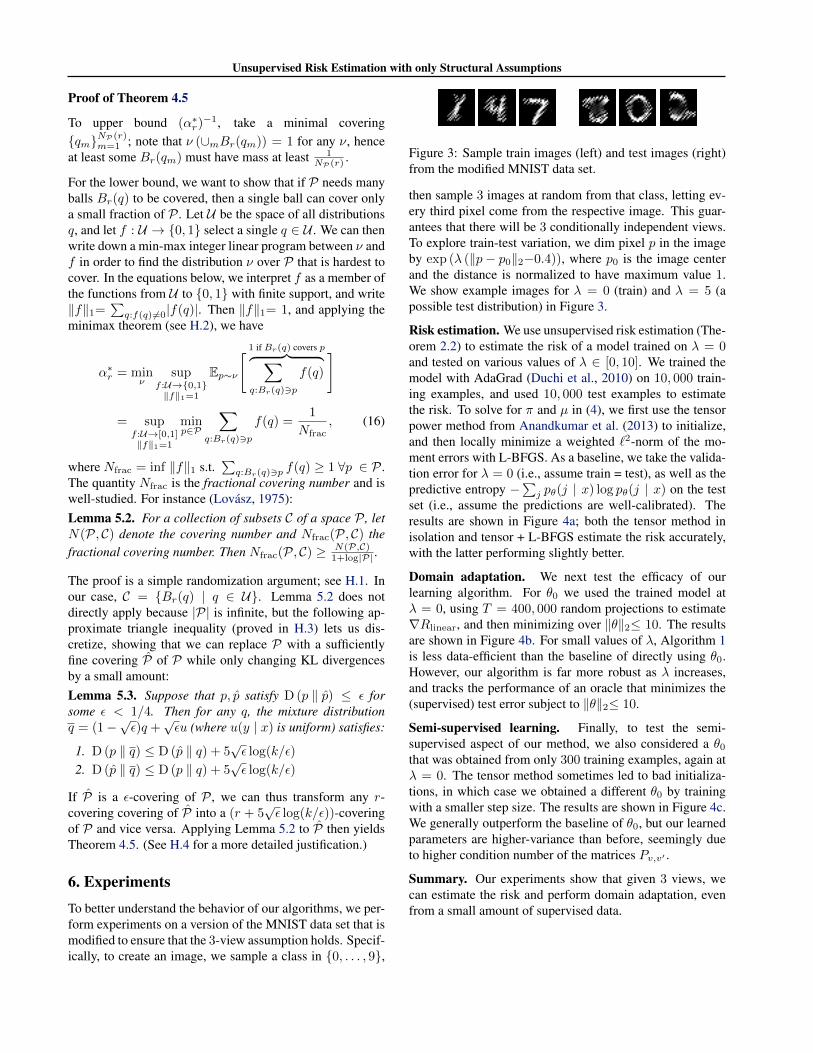
Figure 3: Sample train images (left) and test images (right)from the modified MNIST data set.

then sample 3 images at random from that class, letting ev-ery third pixel come from the respective image. This guar-antees that there will be 3 conditionally independent views.To explore train-test variation, we dim pixel p in the imageby exp (λ (‖p− p0‖2−0.4)), where p0 is the image centerand the distance is normalized to have maximum value 1.We show example images for λ = 0 (train) and λ = 5 (apossible test distribution) in Figure 3.

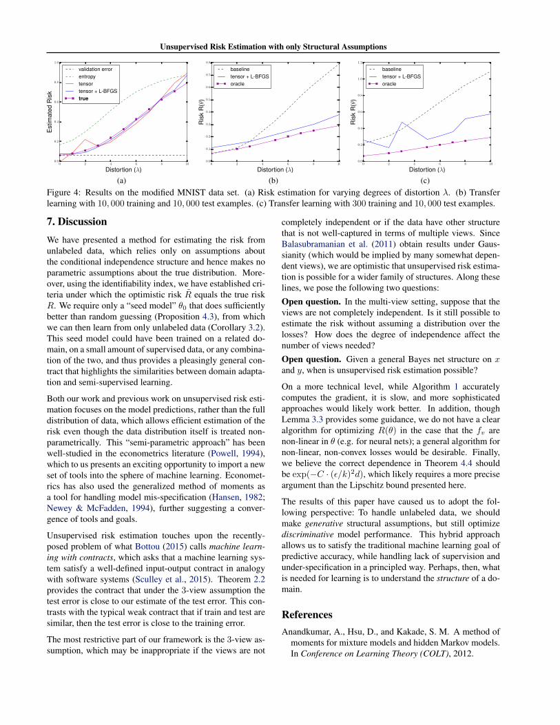
Risk estimation. We use unsupervised risk estimation (The-orem 2.2) to estimate the risk of a model trained on λ = 0and tested on various values of λ ∈ [0, 10]. We trained themodel with AdaGrad (Duchi et al., 2010) on 10, 000 train-ing examples, and used 10, 000 test examples to estimatethe risk. To solve for π and µ in (4), we first use the tensorpower method from Anandkumar et al. (2013) to initialize,and then locally minimize a weighted `2-norm of the mo-ment errors with L-BFGS. As a baseline, we take the valida-tion error for λ = 0 (i.e., assume train = test), as well as thepredictive entropy −

∑j pθ(j | x) log pθ(j | x) on the test

set (i.e., assume the predictions are well-calibrated). Theresults are shown in Figure 4a; both the tensor method inisolation and tensor + L-BFGS estimate the risk accurately,with the latter performing slightly better.

Domain adaptation. We next test the efficacy of ourlearning algorithm. For θ0 we used the trained model atλ = 0, using T = 400, 000 random projections to estimate∇Rlinear, and then minimizing over ‖θ‖2≤ 10. The resultsare shown in Figure 4b. For small values of λ, Algorithm 1is less data-efficient than the baseline of directly using θ0.However, our algorithm is far more robust as λ increases,and tracks the performance of an oracle that minimizes the(supervised) test error subject to ‖θ‖2≤ 10.

Semi-supervised learning. Finally, to test the semi-supervised aspect of our method, we also considered a θ0

that was obtained from only 300 training examples, again atλ = 0. The tensor method sometimes led to bad initializa-tions, in which case we obtained a different θ0 by trainingwith a smaller step size. The results are shown in Figure 4c.We generally outperform the baseline of θ0, but our learnedparameters are higher-variance than before, seemingly dueto higher condition number of the matrices Pv,v′ .

Summary. Our experiments show that given 3 views, wecan estimate the risk and perform domain adaptation, evenfrom a small amount of supervised data.


0 2 4 6 8 10

Distortion (λ)0.0

0.2

0.4

0.6

0.8

1.0

Est

imat

edR

isk

validation errorentropytensortensor + L-BFGStrue

(a)

0 2 4 6 8 10

Distortion (λ)0.0

0.1

0.2

0.3

0.4

0.5

0.6

0.7

0.8

Ris

kR

(θ)

baselinetensor + L-BFGSoracle

(b)

0 2 4 6 8 10

Distortion (λ)0.0

0.2

0.4

0.6

0.8

1.0

1.2

Ris

kR

(θ)

baselinetensor + L-BFGSoracle

(c)Figure 4: Results on the modified MNIST data set. (a) Risk estimation for varying degrees of distortion λ. (b) Transferlearning with 10, 000 training and 10, 000 test examples. (c) Transfer learning with 300 training and 10, 000 test examples.

7. DiscussionWe have presented a method for estimating the risk fromunlabeled data, which relies only on assumptions aboutthe conditional independence structure and hence makes noparametric assumptions about the true distribution. More-over, using the identifiability index, we have established cri-teria under which the optimistic risk R equals the true riskR. We require only a “seed model” θ0 that does sufficientlybetter than random guessing (Proposition 4.3), from whichwe can then learn from only unlabeled data (Corollary 3.2).This seed model could have been trained on a related do-main, on a small amount of supervised data, or any combina-tion of the two, and thus provides a pleasingly general con-tract that highlights the similarities between domain adapta-tion and semi-supervised learning.

Both our work and previous work on unsupervised risk esti-mation focuses on the model predictions, rather than the fulldistribution of data, which allows efficient estimation of therisk even though the data distribution itself is treated non-parametrically. This “semi-parametric approach” has beenwell-studied in the econometrics literature (Powell, 1994),which to us presents an exciting opportunity to import a newset of tools into the sphere of machine learning. Economet-rics has also used the generalized method of moments asa tool for handling model mis-specification (Hansen, 1982;Newey & McFadden, 1994), further suggesting a conver-gence of tools and goals.

Unsupervised risk estimation touches upon the recently-posed problem of what Bottou (2015) calls machine learn-ing with contracts, which asks that a machine learning sys-tem satisfy a well-defined input-output contract in analogywith software systems (Sculley et al., 2015). Theorem 2.2provides the contract that under the 3-view assumption thetest error is close to our estimate of the test error. This con-trasts with the typical weak contract that if train and test aresimilar, then the test error is close to the training error.

The most restrictive part of our framework is the 3-view as-sumption, which may be inappropriate if the views are not

completely independent or if the data have other structurethat is not well-captured in terms of multiple views. SinceBalasubramanian et al. (2011) obtain results under Gaus-sianity (which would be implied by many somewhat depen-dent views), we are optimistic that unsupervised risk estima-tion is possible for a wider family of structures. Along theselines, we pose the following two questions:

Open question. In the multi-view setting, suppose that theviews are not completely independent. Is it still possible toestimate the risk without assuming a distribution over thelosses? How does the degree of independence affect thenumber of views needed?

Open question. Given a general Bayes net structure on xand y, when is unsupervised risk estimation possible?

On a more technical level, while Algorithm 1 accuratelycomputes the gradient, it is slow, and more sophisticatedapproaches would likely work better. In addition, thoughLemma 3.3 provides some guidance, we do not have a clearalgorithm for optimizing R(θ) in the case that the fv arenon-linear in θ (e.g. for neural nets); a general algorithm fornon-linear, non-convex losses would be desirable. Finally,we believe the correct dependence in Theorem 4.4 shouldbe exp(−C · (ε/k)2d), which likely requires a more preciseargument than the Lipschitz bound presented here.

The results of this paper have caused us to adopt the fol-lowing perspective: To handle unlabeled data, we shouldmake generative structural assumptions, but still optimizediscriminative model performance. This hybrid approachallows us to satisfy the traditional machine learning goal ofpredictive accuracy, while handling lack of supervision andunder-specification in a principled way. Perhaps, then, whatis needed for learning is to understand the structure of a do-main.

ReferencesAnandkumar, A., Hsu, D., and Kakade, S. M. A method of

moments for mixture models and hidden Markov models.In Conference on Learning Theory (COLT), 2012.


Anandkumar, A., Ge, R., Hsu, D., Kakade, S. M., and Tel-garsky, M. Tensor decompositions for learning latent vari-able models. arXiv, 2013.

Ando, R. K. and Zhang, T. Two-view feature generationmodel for semi-supervised learning. In Conference onLearning Theory (COLT), pp. 25–32, 2007.

Balasubramanian, K., Donmez, P., and Lebanon, G. Un-supervised supervised learning II: Margin-based classifi-cation without labels. Journal of Machine Learning Re-search (JMLR), 12:3119–3145, 2011.

Balcan, M. and Blum, A. A discriminative model for semi-supervised learning. Journal of the ACM (JACM), 57(3),2010.

Blitzer, J., Kakade, S., and Foster, D. P. Domain adapta-tion with coupled subspaces. In Artificial Intelligence andStatistics (AISTATS), pp. 173–181, 2011.

Blum, A. and Mitchell, T. Combining labeled and unlabeleddata with co-training. In Conference on Learning Theory(COLT), 1998.

Bottou, L. Two high stakes challenges in machine learn-ing. Invited talk at the 32nd International Conference onMachine Learning, 2015.

Boucheron, S., Lugosi, G., and Massart, P. Concentrationinequalities: A nonasymptotic theory of independence.Oxford University Press, 2013.

Cozman, F. and Cohen, I. Risks of semi-supervised learning:How unlabeled data can degrade performance of genera-tive classifiers. In Semi-Supervised Learning. 2006.

Dawid, A. P. and Skene, A. M. Maximum likelihood es-timation of observer error-rates using the EM algorithm.Applied Statistics, 1:20–28, 1979.

Duchi, J., Hazan, E., and Singer, Y. Adaptive subgradientmethods for online learning and stochastic optimization.In Conference on Learning Theory (COLT), 2010.

Edmonds, J. and Karp, R. M. Theoretical improvements inalgorithmic efficiency for network flow problems. Jour-nal of the ACM (JACM), 19(2):248–264, 1972.

Halko, N., Martinsson, P., and Tropp, J. Finding structurewith randomness: Probabilistic algorithms for construct-ing approximate matrix decompositions. SIAM Review,53:217–288, 2011.

Halpern, Y. and Sontag, D. Unsupervised learning of noisy-or Bayesian networks. In Uncertainty in Artificial Intelli-gence (UAI), 2013.

Hansen, L. P. Large sample properties of generalizedmethod of moments estimators. Econometrica: Journalof the Econometric Society, 50:1029–1054, 1982.

Jaffe, A., Nadler, B., and Kluger, Y. Estimating the accura-cies of multiple classifiers without labeled data. In Arti-ficial Intelligence and Statistics (AISTATS), pp. 407–415,2015.

Joachims, T. Transductive inference for text classificationusing support vector machines. In International Confer-ence on Machine Learning (ICML), 1999.

Kakade, S. M. and Foster, D. P. Multi-view regression viacanonical correlation analysis. In Conference on LearningTheory (COLT), pp. 82–96, 2007.

Kolmogorov, A. N. and Tikhomirov, V. M. ε-entropy andε-capacity of sets in function spaces. Uspekhi Matem-aticheskikh Nauk, 14(2):3–86, 1959.

Li, Y. and Zhou, Z. Towards making unlabeled data neverhurt. IEEE Transactions on Pattern Analysis and MachineIntelligence, 37(1):175–188, 2015.

Liang, P. and Klein, D. Analyzing the errors of unsupervisedlearning. In Human Language Technology and Associa-tion for Computational Linguistics (HLT/ACL), 2008.

Lorentz, G. G. Metric entropy and approximation. Bul-letin of the American Mathematical Society, 72(6):903–937, 1966.

Lovasz, L. On the ratio of optimal integral and fractionalcovers. Discrete Mathematics, 13(4):383–390, 1975.

Merialdo, B. Tagging English text with a probabilisticmodel. Computational Linguistics, 20:155–171, 1994.

Nesterov, Y. and Spokoiny, V. Random gradient-free mini-mization of convex functions. Foundations of Computa-tional Mathematics, pp. 1–40, 2011.

Newey, W. K. and McFadden, D. Large sample estimationand hypothesis testing. In Handbook of Econometrics,volume 4, pp. 2111–2245. 1994.

Platanios, E. A. Estimating accuracy from unlabeled data.Master’s thesis, Carnegie Mellon University, 2015.

Powell, J. L. Estimation of semiparametric models. InHandbook of Econometrics, volume 4, pp. 2443–2521.1994.

Quinonero-Candela, J., Sugiyama, M., Schwaighofer, A.,and Lawrence, N. D. Dataset shift in machine learning.The MIT Press, 2009.


Sculley, D., Holt, G., Golovin, D., Davydov, E., Phillips,T., Ebner, D., Chaudhary, V., Young, M., Crespo, J., andDennison, D. Hidden technical debt in machine learningsystems. In Advances in Neural Information ProcessingSystems (NIPS), pp. 2494–2502, 2015.

Shimodaira, H. Improving predictive inference under co-variate shift by weighting the log-likelihood function.Journal of Statistical Planning and Inference, 90:227–244, 2000.

Sion, M. On general minimax theorems. Pacific journal ofmathematics, 8(1):171–176, 1958.

Tomizawa, N. On some techniques useful for solution oftransportation network problems. Networks, 1(2):173–194, 1971.

Tropp, J. A. User-friendly tail bounds for sums of randommatrices. Foundations of computational mathematics, 12(4):389–434, 2012.

Tsirelson, B. S., Ibragimov, I. A., and Sudakov, V. N. Normsof Gaussian sample functions. In Proceedings of the ThirdJapan-USSR Symposium on Probability Theory, pp. 20–41, 1976.

Zhang, Y., Chen, X., Zhou, D., and Jordan, M. I. Spec-tral methods meet EM: A provably optimal algorithm forcrowdsourcing. arXiv, 2014.


A. Details of Computing R from µ

In this section we show how, given A, µ, and π, we can efficiently compute

R(θ) = A(θ)− maxσ∈Sym(k)

k∑j=1

πσ(j)

3∑v=1

(µσ(j),v)j . (17)

The only bottleneck is the maximum over σ ∈ Sym(k), which would naıvely require considering k! possibilities. However,we can instead cast this as a form of maximum matching. In particular, form the k × k matrix

Xi,j = πi

3∑v=1

(µi,v)j . (18)

Then we are looking for the permutation σ such that∑kj=1Xσ(j),j is maximized. If we consider each Xi,j to be the weight

of edge (i, j) in a complete bipartite graph, then this is equivalent to asking for a matching of i to j with maximum weight,hence we can maximize over σ using any maximum-weight matching algorithm such as the Hungarian algorithm, which runsin O

(k3)

time (Tomizawa, 1971; Edmonds & Karp, 1972).

B. Proof of Theorem 2.2Preliminary reductions. Our goal is to estimate R to error ε (with probability of failure 1− δ) in poly

(k, π−1

min, λ−1, τ

)·

log(1/δ)ε2 samples. Since R is a scalar parameter, if we can estimate R to error ε with any fixed probability of success

1 − δ0 > 1/2, then by taking the median of O (log(1/δ)/δ0) independent estimates, we can amplify the probability ofsuccess to 1− δ. In this argument we will focus on achieving a probability of success of 3/4.

Letting Rσlinear be the linear part of the risk if the labels are permuted by σ, note that

R = A−minσRσlinear (19)

= A−minσ

k∑j=1

πσ(j)

3∑v=1

(µσ(j),v)j (20)

Note that 0 ≤ πσ(j) ≤ 1 and −τ ≤ (µσ(j),v)j ≤ τ . Therefore, as long as each of the quantities (A, π, µ) can be estimated toerror ε in poly

(k, π−1

min, λ−1, τ

)/ε2 samples, by taking an appropriately scaled down ε (roughly kτ times smaller to account

for the product terms of π with µ), we can estimate the entire expression for R to within error ε as well. We therefore focusthe remainder of the argument on estimating A, π, and µ individually.

Estimatimg A. Remember that A = Ex[A(θ;x)], and that Ex[A2] ≤ τ2 by assumption. Therefore, A can be estimated toerror ε (with probability, say, 11/12) using poly(τ)/ε2 samples.

Estimating µ. Estimating π and µ is mostly an exercise in interpreting Theorem 7 of Anandkumar et al. (2012), which werecall below, modifying the statement slightly to fit our language.

Theorem B.1 (Anandkumar et al. (2012)). Let Pv,v′def= E[hv(x) ⊗ hv′(x)], and P1,2,3

def= E[h1(x) ⊗ h2(x) ⊗ h3(x)].

Also let Pv,v′ and P1,2,3 be sample estimates of Pv,v′ , P1,2,3 that are (for technical convenience) estimated from independentsamples of size m. Let ‖T‖F denote the `2-norm of T after unrolling T to a vector. Suppose that:

• P[‖Pv,v′ − Pv,v′‖2≤ Cv,v′

√log(1/δ)

m

]≥ 1− δ for v, v′ ∈ 1, 2, 1, 3, and

• P[‖P1,2,3 − P1,2,3‖F≤ C1,2,3

√log(1/δ)

m

]≥ 1− δ.


Then, there exists constants C, m0, δ0 such that the following holds: if m ≥ m0 and δ ≤ δ0 and√log(k/δ)

m≤ C · minj 6=j′‖µj,3 − µj′,3‖2·σk(P1,2)

C1,2,3 · k5 · κ(M1)4· δ

log(k/δ)· ε,√

log(1/δ)

m≤ C ·min

minj 6=j′‖µj,3 − µj′,3‖2·σk(P1,2)2

C1,2 · ‖P1,2,3‖F ·k5 · κ(M1)4· δ

log(k/δ),σk(P1,3)

C1,3

· ε,

then with probability at least 1 − 5δ, we can output M3 = [µ1,3 · · · µk,3] with the following guarantee: there exists apermutation σ ∈ Sym(k) such that for all j ∈ 1, . . . , k,

‖µj,3 − µσ(j),3‖2≤ maxj′‖µj′,3‖2·ε. (21)

By symmetry, we can use Theorem B.1 to recover each of the matrices Mv , v = 1, 2, 3, up to permutation of the columns.Furthermore, Anandkumar et al. (2012) show in Appendix B.4 of their paper how to match up the columns of the differentMv , so that only a single unknown permutation is applied to each of the Mv simultaneously. We will set δ = 1/180, whichyields an overall probability of success of 11/12 for this part of the proof.

We now analyze the rate of convergence implied by Theorem B.1. Note that we can take C1,2,3 =

O(√

E[‖h1‖22‖h2‖22‖h3‖22])

, and similarly Cv,v′ = O(√

E[‖hv‖22‖hv′‖22])

. Then, since we only care about polyno-

mial factors, it is enough to note that we can estimate the Mv to error ε given Z/ε2 samples, where Z is polynomial in thefollowing quantities:

1. k,

2. max3v=1 κ(Mv), where κ denotes condition number,

3.√

E[‖h1‖22‖h2‖22‖h3‖22]

(minj,j′‖µj,v−µj′,v‖2)·σk(Pv′,v′′ ), where (v, v′, v′′) is a permutation of (1, 2, 3),

4. ‖P1,2,3‖2(minj,j′‖µj,v−µj′,v‖2)·σk(Pv′,v′′ )

, where (v, v′, v′′) is as before, and

5.√

E[‖hv‖22‖hv′‖22]

σk(Pv,v′).

6. maxj,v‖µj,v‖2.

It suffices to show that each of these quantities are polynomial in k, π−1min, τ , and λ−1.

(1) k is trivially polynomial in itself.

(2) Note that κ(Mv) ≤ σ1(Mv)/λ ≤ ‖Mv‖F /λ. Furthermore, ‖Mv‖2F=∑j‖E[hv | j]‖22≤

∑j E[‖hv‖22| j] ≤ kτ2. In all,

κ(Mv) ≤√kτ/λ, which is polynomial in k and τ/λ.

(3) We first note that minj 6=j′‖µj,v − µj′,v‖2=√

2 minj 6=j′‖Mv(ej − ej′)‖2/‖ej − ej′‖2≥ σk(Mv). Also, σk(Pv′,v′′) =σk(Mv′ diag(π)Mv′′) ≥ σk(Mv′)πminσk(Mv′′). We can thus upper-bound the quantity in (3.) by√

E[‖h1‖22‖h2‖22‖h3‖22]√2πminσk(M1)σk(M2)σk(M3)

≤ τ3

√2πminλ3

,

which is polynomial in π−1min, τ/λ.


(4) We can perform the same calculations as in (3), but now we have to bound ‖P1,2,3‖2. However, it is easy to see that

‖P1,2,3‖2 =√‖E[h1 ⊗ h2 ⊗ h3]‖22

≤√

E[‖h1 ⊗ h2 ⊗ h3‖22]

=√

E[‖h1‖22‖h2‖22‖h3‖22]

=

√√√√ k∑j=1

πj

3∏v=1

E[‖hv‖22| y = j]

≤ τ3,

which yields the same upper bound as in (3).

(5) We can again perform the same calculations as in (3), where we now only have to deal with a subset of the variables, thusobtaining a bound of τ2

πminλ2 .

(6) We have ‖µj,v‖2≤√E[‖hv‖22| y = j] ≤ τ .

In sum, we have shown that with probability 1112 we can estimate each µj,v to `2 error ε using poly

(k, π−1

min, λ−1, τ

)/ε2

samples. It now remains to estimate π.

Estimating π. This part of the argument follows Appendix B.5 of Anandkumar et al. (2012). Noting that π = M−11 E[h1],

we can estimate π as π = M1−1

E[h1], where E denotes the empirical expectation. Hence, we have

‖π − π‖∞ ≤∥∥∥(M1

−1−M−1

1 )E[h1] +M−11 (E[h1]− E[h1]) + (M1

−1−M−1

1 )(E[h1]− E[h1])∥∥∥∞

≤ ‖M1−1−M−1

1 ‖F︸︷︷︸(i)

‖E[h1]‖2︸︷︷︸(ii)

+ ‖M−11 ‖F︸︷︷︸

(iii)

‖E[h1]− E[h1]‖2︸︷︷︸(iv)

+ ‖M1−1−M−1

1 ‖F︸︷︷︸(i)

‖E[h1]− E[h1]‖2︸︷︷︸(iv)

.

We will bound each of these factors in turn:

(i) ‖M1−1− M−1

1 ‖F : let E1 = M1 − M1, which by the previous part satisfies ‖E1‖F≤√kmaxj‖µj,1 − µj,1‖2=

poly(k, π−1

min, λ−1, τ

)/√m. Therefore:

‖M1−1−M−1

1 ‖F ≤ ‖(M1 + E1)−1 −M−11 ‖F

= ‖M−11 (I + E1M

−11 )−1 −M−1

1 ‖F≤ ‖M−1

1 ‖F ‖(I + E1M−11 )−1 − I‖F

≤ kλ−1σ1

(I + E1M

−11 )−1 − I

)≤ kλ−1 σ1(E1M

−11 )

1− σ1(E1M−11 )

≤ kλ−2 ‖E1‖F1− λ−1‖E1‖F

≤poly

(k, π−1

min, λ−1, τ

)1− poly

(k, π−1

min, λ−1, τ

)/√m· 1√

m.

We can assume that m ≥ poly(k, π−1

min, λ−1, τ

)without loss of generality (since otherwise we can trivially obtain

the desired bound on ‖π − π‖∞ by simply guessing the uniform distribution), in which case the above quantity ispoly

(k, π−1

min, λ−1, τ

)· 1√

m.

(ii) ‖E[h1]‖2: we have ‖E[h1]‖2≤√E[‖h1‖22] ≤ τ .

(iii) ‖M−11 ‖F : since ‖X‖F≤

√kσ1(F ), we have ‖M−1

1 ‖F≤√kλ−1.


(iv) ‖E[h1]− E[h1]‖2: with any fixed probability (say 11/12), this term is O(√

E[‖h1‖22]m

)= O

(τ√m

).

In sum, with probability at least 1112 all of the terms are poly

(k, π−1

min, λ−1, τ

), and at least one factor in each term has a 1√

m

decay. Therefore, we have ‖π − π‖∞≤ poly(k, π−1

min, λ−1, τ

)·√

1m .

Since we have shown that we can estimate each of A, π, and µ individually with probability 1112 , we can also estimate R with

probability 34 , thus completing the proof.

C. Proofs of Theorem 3.1 and Corollary 3.2Proof of Theorem 3.1. First, we note that Theorem 2.2 can be extended to the case where instead of just estimating µ, wealso estimate gt = u>t ∇θRlinear. Since re-proving Theorem 3.1 in this case would be tedious, we simply highlight the maindifferences.

First, M is now a 2k × k matrix rather than a k × k matrix; moreover, since all we do to M is add k additional rows, theminimum singular value λ can only increase (which would decrease the sample complexity). On the other hand, τ couldincrease to τ2 + B2 once we add in u>∇θhv . To deal with this, we first scale u>∇θfv down by a factor of B (and thenscale it up afterwards), which is why our final error bound will depend on Bε rather than just ε. Finally, πmin and k remainunchanged. We note that we need the slightly stronger guarantee that Rσ(θ) and u>t ∇θRσlinear are uniformly well-estimatedfor all σ, which is a straightforward consequence of Theorem B.1.

Now, we can assume that for all t = 1, . . . , T (where T = O(d log(d/δ)/ε2

)), we successfully estimate each Rσ to within

error ε/5 with probability 1− δ/2 (where we union bound over t, using the fact that we the number of samples m is requiredto grow with log(T/δ)). Since ε < gap(θ0), we thus necessarily recover the correct permutation σ, and can undo it to obtaingt such that |gt − u>t ∇θRlinear‖≤ ε′, where ε′ = Bε/5. Let εt = gt − u>t ∇θRlinear. We then have∥∥∥∥∥ 1

T

T∑t=1

utgt −∇θRlinear

∥∥∥∥∥2

≤

∥∥∥∥∥ 1

T

T∑t=1

utu>t ∇θRlinear −∇θRlinear

∥∥∥∥∥2

+

∥∥∥∥∥ 1

T

T∑t=1

ut(u>t ∇θRlinear − gt)

∥∥∥∥∥2

=

∥∥∥∥∥ 1

T

T∑t=1

utu>t − I

∥∥∥∥∥op

∥∥∥∇θRlinear

∥∥∥2

+1

T

∥∥∥∥∥T∑t=1

εtut

∥∥∥∥∥2

≤

∥∥∥∥∥ 1

T

T∑t=1

utu>t − I

∥∥∥∥∥op

∥∥∥∇θRlinear

∥∥∥2

+1

T‖[u1 · · · uT ]‖op ‖ε1:T ‖2

≤ 3B

∥∥∥∥∥ 1

T

T∑t=1

utu>t − I

∥∥∥∥∥op

+ ε′

∥∥∥∥∥ 1

T

T∑t=1

utu>t

∥∥∥∥∥12

op

.

Now, by Theorem 1.2 of Tropp (2012), we have for ε < 1 that

P

[σmax

(1

T

T∑t=1

utu>t

)≥ 1 + ε/5

]≤ d exp

(−ε

2T

75d

). (22)

Thus, setting T = 75dε2 log(2d/δ), we get that, with probability 1− δ/2, we have∥∥∥∥∥ 1

T

T∑t=1

utgt −∇θRlinear

∥∥∥∥∥2

≤ 3Bε/5 + 2ε′ = Bε, (23)

as was to be shown.

Proof of Corollary 3.2. Since θ0 ∈ Θ0, we know that ∇θ0Rlinear = ∇θ0Rlinear. Now note that θ> (g −∇θ0Rlinear) ≤‖θ‖2‖g − ∇θ0Rlinear‖2≤ εBρ for all θ with ‖θ‖2≤ ρ. In addition, by standard Rademacher complexity bounds we havewith probability 1 − δ that ‖A(θ) − 1

m

∑mi=1A(θ;x(i))‖2≤ εBρ for all ‖θ‖2≤ ρ, provided that m = Ω

(log(1/δ)

ε2

), since

A(θ;x(i)) is B-Lipschitz. Putting these together, the result follows by a standard uniform convergence argument.


D. Proof of Lemma 3.3Recall that we are given θ0 ∈ Θ0, and θ such that Ex∼p∗

[maxkj=1|f(θ;x, j)− f(θ0;x, j)|

]≤ 1

2 (gap(θ) + gap(θ0)). Ourgoal is to show that θ ∈ Θ0 as well.

By the definition of gap(θ0), we have Rσ(θ0) ≥ R(θ0) + gap(θ0) for all σ 6= id. Assume for the sake of contradiction thatR(θ) 6= R(θ); then again by the definition of gap, there exists a σ 6= id with Rσ(θ) ≤ R(θ)− gap(θ).

To derive a contradiction, we will study Rlinear and Rσlinear. We have that

Rlinear(θ0) ≤ Rσlinear(θ0)− gap(θ0) (24)≤ |Rσlinear(θ0)−Rσlinear(θ)|+Rσlinear(θ)− gap(θ0) (25)≤ |Rσlinear(θ0)−Rσlinear(θ)|+Rlinear(θ)− (gap(θ0) + gap(θ)) (26)≤ |Rσlinear(θ0)−Rσlinear(θ)|+|Rlinear(θ0)−Rlinear(θ)|+Rlinear(θ0)− (gap(θ0) + gap(θ)) . (27)

On the other hand, for all permutations σ we have:

|Rσlinear(θ0)−Rσlinear(θ)| =

∣∣∣∣∣∣k∑j=1

πjE[f(θ0;x, σ(j))− f(θ;x, σ(j)) | y = j]

∣∣∣∣∣∣ (28)

≤k∑j=1

πjE[

kmaxj′=1|f(θ0;x, j′)− f(θ;x, j′)|

∣∣∣ y = j

](29)

= E[

kmaxj′=1|f(θ0;x, j′)− f(θ;x, j′)|

](30)

<1

2(gap(θ) + gap(θ0)) . (31)

Substituting this in for both Rσlinear and Rlinear = Ridlinear in (27) above yields the desired contradiction and hence completes

the proof.

E. Proof of Proposition 4.3First, suppose that p∗ ∼ ν′. Note that (µj)j − (µj)j′ measures how much larger E[− log pθ(j | x) | y = j] would becomeif we assign class j to label j′. Therefore, the condition γ(θ) > 0 implies that E[− log pθ(j

′ | x) | y = j] > E[− log pθ(j |x) | y = j] for all j 6= j′. Therefore, any σ 6= id will have Rσ(θ) > R(θ), and so R(θ) = R(θ).

Next, suppose that p∗ ∼ ν. Then, we have

P[R(θ) ≤ r0] = P[minσRσ(θ) ≤ r0] (32)

= P[minσ

E[− log pθ(σ(y) | x)] ≤ r0] (33)

≤ P[minσ

D (pθ(σ(y) | x) ‖ p∗(y | x)) ≤ r0] (34)

≤∑σ

P[D (pθ(σ(y) | x) ‖ p∗(y | x)) ≤ r0] (35)

≤ k!αr0 . (36)

Putting these together, we havemax

ν∈ν,ν′Pν [R(θ) ≤ r0 ∧ R(θ) 6= R(θ)] ≤ k!αr0 , (37)

as was to be shown.

F. Extension of Proposition F.1In this section, we establish the following extension of Proposition F.1:


Proposition F.1. Suppose that p∗ ∼ ν. Then for any 0 < ε < 2, we have the uniform false negative bound

P[∃θ, R(θ) < r0] ≤ k!NΘ((ε/4√k)4)αr0+ε, (38)

where NΘ is the covering number of Θ under D (· ‖ ·).

Note that NΘ is typically exponential in the dimension of Θ; comparing to e.g. Theorem 4.4 below, we thus need Θ to havesmaller dimension than the model family of p∗ for (38) to be non-trivial (which could be true in e.g. transfer learning settingswhere we tune a subset of the parameters to a new domain).

Proof of Proposition F.1. We want to boundP[∃θ ∈ Θ, R(θ) ≤ r0]. (39)

To start, let Q be a minimal covering of Θ under D (· ‖ ·) of radius ε0, where ε0 will be chosen later. We will replace eachq ∈ Q with the distribution q = (1− δ)q + δu, where u is the uniform distribution and δ > 0 will also be chosen later. LetQ denote this new set of distributions.

By the same logic as Proposition 4.3, the probability that minq∈Q R(q) ≤ r0 + ε is at most k! |Q|αr0+ε. We would now liketo use this to say something about Θ. We will be able to do so with the following lemma:

Lemma F.2. Suppose that D (p ‖ q) ≤ ε0. Then, for all distributions p∗,

D (p∗ ‖ q) ≤ D (p∗ ‖ p) + log

(1

1− δ

)+ (k/δ)

√ε0/2. (40)

Roughly, this says: “if q covers p and p covers p∗, then q covers p∗”. For our purposes, we will set δ =√k(ε0/8)1/4.

Assuming that δ ≤ 1/2, we have the bound log 11−δ ≤ 2δ, so that Lemma F.2 would imply the bound D (p∗ ‖ q) ≤

D (p∗ ‖ p) + 2√k(2ε0)1/4.

To apply Lemma F.2, consider the event E that minθ∈Θ R(θ) ≤ r0. In the following argument, we will let pσ denote thedistribution with pσ(y | x) = p(σ(y) | x).

The eventE implies that there exists pθ, σ with D (p∗ ‖ pσθ ) ≤ r0, and becauseQ covers Θ, there is also a q with D (pθ ‖ q) ≤ε0 (and hence also D (pσθ ‖ qσ) ≤ ε0). Invoking Lemma F.2, there is thus a q ∈ Q such that D (p∗ ‖ qσ) ≤ r0 +2

√k(2ε0)1/4.

We will now choose ε0 = (ε/4√k)4, which is enough to ensure that D (p∗ ‖ qσ) ≤ r0 + ε; hence P[E] ≤ P[minq∈Q R(q) ≤

r0 + ε] ≤ k! |Q|αr0+ε, as was to be shown.

Two remaining details are to check that δ < 1/2, and to prove Lemma F.2. For the first, since δ =√k(ε0/8)1/4 <√

k(ε/4√k) = ε/4, it suffices to constrain ε < 2, which we assumed. We now turn to Lemma F.2.

Proof of Lemma F.2. We will first prove the equivalent result for KL divergence KL (· ‖ ·) (instead of the averaged KLdivergence D (· ‖ ·)). Note that

KL (p∗ ‖ q)−KL (p∗ ‖ p) = Ep∗[log

p(x)

q(x)

]≤ Ep∗

[max

(log

p(x)

q(x), 0

)](i)

≤ k

δEq[max

(log

p(x)

q(x), 0

)](ii)

≤ k

δEq[max

(p(x)− q(x)

q(x), 0

)]=k

δ‖p− q‖TV

≤ k

δ‖p− q‖TV ,


where (i) uses the fact that p∗ ≤ (k/δ)q and (ii) uses log(a/b) ≤ (a − b)/b for a ≥ b. We then note that ‖p − q‖TV≤√KL (p ‖ q) /2 by Pinsker’s inequality, and also that KL (p∗ ‖ p) ≤

∫p∗(x) log p∗(x)

(1−δ)p(x)dx ≤ KL (p∗ ‖ p) + log(

11−δ

).

Averaging over x ∼ π, we have

D (p∗ ‖ q) ≤ D (p∗ ‖ p) + log

(1

1− δ

)+ (k/δ)Ex∼π

[√KL (p(Y | x) ‖ q(Y | x))

](41)

≤ D (p∗ ‖ p) + log

(1

1− δ

)+ (k/δ)

√D (p ‖ q) /2, (42)

which completes the proof.

G. Justification of Some Details for Theorem 4.4G.1. Treating pβ as a point mass

Here we justify why, for sufficiently large τ , if each βj ∼ N (0, ·Id×d), then we can treat pβ,τ (Y = j | x) ∝ exp(τβ>j φ(x)

)as a point mass. Precisely, we have the following result:

Lemma G.1. Let βj ∼ N (0, Id×d). For any τ , let

pβ,τ (Y = j | x) ∝ exp(τ · β>j φ(x)

), and let pβ,∞(Y = j | x)

def= I

[j = arg max

j′β>j′φ(x)

]. (43)

Then, if F is the family of functions f : X × Y → [−1, 1], we have, for every δ > 0,

limτ→∞

Pβ1:k∼N (0,I)

[supf∈F

Epβ,τ [f(x, y)]− Epβ,∞ [f(x, y)] > δ

]= 0 (44)

In particular, since in light of (13) we only need to worry about the expectation of q(y | x), which itself lies in [0, 1], for anydesired error threshold δ the probability that the difference between Epβ,τ [q(y | x)] and Epβ,∞ [q(y | x)] exceeds δ goes to 0uniformly (in q) as τ →∞. Since the constants we provide in Theorem 4.4 are slightly larger than those actually implied byour proofs, there is some non-infinite value of τ that implies Theorem 4.4 with the stated constants, even though we otherwiseonly establish the result for pβ,∞.

Proof of Lemma G.1. Note that the supremum in (44) is simply the expected total variational distanceEx∼π [‖pβ,τ (Y | x)− pβ,∞(Y | x)‖TV ]. We then have

limτ→∞

Pβ1:k∼N (0,I) [Ex∼π [‖pβ,τ (Y | x)− pβ,∞(Y | x)‖TV ] > δ] (45)

≤ δ−1 limτ→∞

Eβ1:k,x [‖pβ,τ (Y | x)− pβ,∞(Y | x)‖TV ] (46)

(i)= 0. (47)

To justify (i), note that since φ(x) 6= 0 almost surely, pβ,τ (y | x) → pβ,∞(y | x) almost surely as τ → ∞. Since totalvariational distance is bounded by 1, by Lebesgue’s dominated convergence theorem, the limit of the expectation is indeedzero.


G.2. Approximating π by samples

Applying Lebesgue’s dominated convergence theorem at (i) below, we have

limm→∞

Pβ,x1:m

[1

m

m∑i=1

q(yβ(xi) | xi) ≥1 + ε

k

]= limm→∞

Eβ,x1,x2,...

[I

[1

m

m∑i=1

q(yβ(xi) | xi) ≥1 + ε

k

]](48)

(i)= Eβ,x1,x2,...

[limm→∞

I

[1

m

m∑i=1

q(yβ(xi) | xi) ≥1 + ε

k

]](49)

= Eβ,x1,x2,...

[I[Ex∼π[q(yβ(x) | x)] ≥ 1 + ε

k

]](50)

= Pβ[Ex∼π[q(yβ(x) | x)] ≥ 1 + ε

k

]. (51)

G.3. Computing Lipschitz constants

Recall we want to show that the map β1:k 7→ t1:m1:k is ‖Φ‖op-Lipschitz, and that the map (q(yβ(xi) | xi))mi=1 7→

1m

∑mi=1 q(yβ(xi) | xi) is (1/

√m)-Lipschitz.

In the first case, remember that tij is defined to be β>j φ(xi)/‖φ(xi)‖2. Therefore, the map β 7→ t is in fact linear, withcorresponding matrix Φ>. The Lipschitz constant of a linear map is simply its operator norm, i.e. ‖Φ‖op, as claimed.

In the second case, our map is again linear, and is equivalent to the map v 7→ (1/m)1>v, where v ∈ Rm. This map hasLipschitz constant (1/m)‖1‖2= 1/

√m, again as claimed.

G.4. Modifying q to be Lipschitz

Let us be a bit more formal about how we modify q. We will define the function

rβ(x)def=

k∑j=1

max

(0, 1− 1

δ

kmaxi=1

(βi − βj)>φ(x)

‖φ(x)‖2

)q(Y = j | x). (52)

Therefore, rβ(x) ≥ q(yβ(x) | x) always, and will be bigger if there are other values βi such that β>i φ(x) is close to themaximum.

Note that (βi − βj)> φ(x)‖φ(x)‖2 is

√2-Lipschitz, hence each term is

√2δ q(Y = j | x)-Lipschitz; since

∑j q(Y = j | x) = 1,

the entire expression is√

2δ -Lipschitz, as claimed. We also have the following bound on its expectation:

Lemma G.2. For any x, if β1:k ∼ N (0, I), then

Eβ [rβ(x)] ≤ 1

k+ δ. (53)

Proof. Since∑kj=1 q(Y = j | x) = 1, it suffices to show that for each j,

E[max

(0, 1− δ−1 max

i(βi − βj)>

φ(x)

‖φ(x)‖2

)]≤ 1

k+ δ. (54)

Let ti = β>iφ(x)‖φ(x)‖2 ; note that the ti are independent Gaussians with mean zero and variance 1. Note also that the term in

the expectation is always at most 1, and is only non-zero if either (i) tj is the largest of the ti (which occurs with probability1/k) or if (ii) M < tj < M + δ, where M = maxi 6=j ti. Conditioned on M , this latter event always has probability at mostδ√2π

< δ (since the density of a Gaussian is bounded everywhere by 1√2π

). Marginalizing over M , the overall probability isalso at most δ, and so the overall expectation in (54) is at most 1

k + δ, as was to be shown.


G.5. Obtaining the final bound

Take δ = ε2k , so that E[rβ(x)] ≤ 1+ε/2

k . Also define r = 1m

∑mi=1 rβ(xi). Then, since q(yβ(x) | x) ≤ rβ(x) (see the

remarks in G.4), we have

Pβ

[1

m

m∑i=1

q(yβ(xi) | xi) ≥1 + ε

k

]≤ Pβ

[1

m

m∑i=1

rβ(xi) ≥1 + ε

k

](55)

= Pβ[r ≥ 1 + ε

k

](56)

≤ Pβ [r − E[r] ≥ ε

2k] (57)

≤ exp

(− ε4

64k4

m

‖Φ‖2op

), (58)

where the final line invokes Theorem 5.1, using the fact that β 7→ r is (‖Φ‖op·(2√

2k/ε) · (1/√m))-Lipschitz.

G.6. Almost sure convergence

We have

limm→∞

Pβ,x1:m

[1

m

m∑i=1

q(yβ(xi) | xi) ≥1 + ε

k

](59)

(58)≤ lim

m→∞Ex1:m

[exp

(− ε4

64k4

m

‖Φ(x1:m)‖2op

)](60)

(i)= Ex1,x2,...

[limm→∞

exp

(− ε4

64k4

m

‖Φ(x1:m)‖2op

)](61)

(ii)= exp

(− ε4

64k4γ−1

), (62)

where (i) is Lebesgue’s dominated convergence theorem and (ii) is because ‖Φ‖2op/m→ γ−1 almost surely as m→∞.

H. Justification of Some Details for Theorem 4.5H.1. Proof of Lemma 5.2

Let f : C → [0, 1] be an optimal fractional covering. For t = 1, . . . , T , sample St ∈ C with probability f(St)Nfrac

. Thenfor any fixed t and p ∈ P , we have P[p is covered by St] ≥ 1

Nfrac. After T = dNfrac log|P|e samples, we thus have

P[p is not covered by any St] ≤ (1 − 1Nfrac

)Nfrac log|P| < e− log|P| = 1|P| . So with non-zero probability, we cover all p ∈ P

after dNfrac log|P|e samples, and so N ≤ dNfrac log|P|e ≤ Nfrac(log|P|+1).


H.2. Applying the minimax theorem

To expand on (16), we have

α∗r = minν

supf :U→0,1‖f‖1=1

Ep∼ν

[ 1 ifBr(q) covers p︷︸︸︷∑q:Br(q)3p

f(q)

]

(i)

≤ minν

supf :U→[0,1]‖f‖1=1

Ep∼ν

[ ∑q:Br(q)3p

f(q)

]

(ii)= sup

f :U→[0,1]‖f‖1=1

minν

Ep∼ν

[ ∑q:Br(q)3p

f(q)

]

= supf :U→[0,1]‖f‖1=1

minp∈P

∑q:Br(q)3p

f(q) =1

Nfrac,

Here (i) just relaxes the integer program to a linear program, and (ii) applies the following minimax theorem, which isTheorem 4.1 of Sion (1958):

Theorem H.1. LetX and Y be any spaces, h a function onX×Y that is concave-convexlike. If for any c < infy supx h(x, y)there exists a finite set X0 ⊂ X such that infy maxx∈X0

h(x, y) > c, then infy supx h(x, y) = supx infy h(x, y).

Here concave-convexlike is defined as follows: (i) for every x1, x2 ∈ X and t ∈ [0, 1], there is a x0 ∈ X such thatt · h(x1, y) + (1− t) · h(x2, y) ≤ h(x0, y) for all y ∈ Y ; (ii) for every y1, y2 ∈ Y and t ∈ [0, 1], there is a y0 ∈ Y such thatt · h(x, y1) + (1− t) · h(x, y2) ≥ h(x, y0) for all x ∈ X .

We intend to apply Theorem H.1 with X = Ffinite(U ; 1) (the space of finitely supported functions from U to [0, 1] satisfying‖f‖1= 1), Y = ∆(P) (the space of probability distributions on P), and h(f, ν) = Ep∼ν

[∑q:Br(q)3p f(q)

].

First, we check the convexity and concavity properties. Given ν1, ν2 ∈ ∆(P) and t ∈ [0, 1], we can clearly take ν0 =tν1 + (1 − t)ν2. Similarly, given f1, f2 ∈ Ffinite(U ; 1) and t ∈ [0, 1], we can clearly take f0 = tf1 + (1 − t)f2, which isfinitely supported if f1 and f2 are.

Next, take some c < infν∈∆(P) supf∈Ffinite(U ;1) h(f, ν). This means that in particular, c < infν∈∆(P) supq ν(Br(q)) = α∗r .Since α∗r is continuous by assumption, we thus also have that c < infν∈∆(P) supq ν(Bq(r − δ)) for some δ > 0. Now,for some ε (to be determined later), take a finite ε4-covering q1, . . . , qN of P , and also set qn = (1 − ε)qn + εu, whereu is the uniform distribution. We claim that minNn=1 ν(Br(qn)) > c for all ν ∈ ∆(P), whence we can take the functionsfn = I[q = qn] and X0 = fnNn=1 to satisfy the conditions of Theorem H.1.

To show this, we will show that for each q, Br−δ(q) ⊆ Br(qn) for some n, so that supq ν(Br−δ(q)) ≤ maxnn=1 ν(Br(qn)).Indeed, take n such that D (q ‖ qn) ≤ ε4. By Lemma F.2, we then have that for any p ∈ Br−δ(q), D (p ‖ qn) ≤ D (p ‖ q) +

log(

11−ε

)+ (k/ε)

√ε4/2. Since D (p ‖ q) ≤ r − δ, we can ensure that D (p ‖ qn) ≤ r for sufficiently small ε, as claimed.

H.3. Proof of Lemma 5.3

As before, let p = (1− δ)p + δu, where u is the uniform distribution; we will take δ =√ε. We will make extensive use of

the following helper lemma regarding the behavior of p, proved later in this section:

Lemma H.2. Let H(δ) = δ log(

1δ

)+ (1− δ) log

(1

1−δ

). Also suppose that δ < 1

2 . Then, for any p and q, we have:

KL (p ‖ q) ≤ KL (p ‖ q) + log

(1

1− δ

)(63)

KL (q ‖ p) ≥ (1− δ) KL (p ‖ q)−H(δ) (64)KL (p ‖ q) ≤ (1− δ) KL (p ‖ q) +H(δ) (65)KL (p ‖ q) ≤ 2(1− δ)‖p− q‖TV log(k/δ). (66)


Also under the assumption δ < 1/2, we have log(1/(1 − δ)) ≤ 2δ, which we will often use to simplify some of the aboveexpressions. Now, starting with the actual proof, we have

KL (p ‖ q) = KL(p ‖ q

)+(KL (p ‖ q)−KL

(p ‖ q

))(65)≤ (1− δ) KL (p ‖ q) +H(δ) +

(KL (p ‖ q)−KL

(p ‖ q

)).

Furthermore, we have

KL (p ‖ q)−KL(p ‖ q

)=

∫p(x) log

p(x)

q(x)dx−

∫p(x) log

p(x)

q(x)dx

= KL(p ‖ p

)+

∫(p(x)− p(x)) log

p(x)

q(x)dx

≤ KL(p ‖ p

)+

∣∣∣∣∫ (p(x)− p(x))dx

∣∣∣∣ log(k/δ)

≤ KL (p ‖ p) + 2δ + 2‖p− p‖TV log(k/δ)

≤ KL (p ‖ p) + 2δ + 2(‖p− p‖TV +‖p− p‖TV ) log(k/δ)

≤ ε+ 2δ + 2(√ε/2 + δ) log(k/δ),

in which case

KL (p ‖ q) ≤ (1− δ) KL (p ‖ q) + ε+√

2ε log(k/δ) +H(δ) + 2δ (log(k/δ) + 1)

≤ KL (p ‖ q) +√ε(

(√

2 + 2) log(k) + (√

2 + 3) log(1/√ε) + 4 +

√ε)

≤ KL (p ‖ q) + 5√ε log(2k/ε).

For the second part, by symmetry we will suppose instead that KL (p ‖ p) ≤ ε and prove the same inequality as before. Wehave

KL (p ‖ q) = KL (p ‖ q) + (KL (p ‖ q)−KL (p ‖ q)) + (KL (p ‖ q)−KL (p ‖ q)) + (KL (p ‖ q)−KL (p ‖ q))≤ KL (p ‖ q) + 2δ +H(δ) + δKL (p ‖ q) + (KL (p ‖ q)−KL (p ‖ q))≤ KL (p ‖ q) + 2δ +H(δ) + δ log(k/δ) + (KL (p ‖ q)−KL (p ‖ q)) .

Using essentially the same argument as before, we have

KL (p ‖ q)−KL (p ‖ q) =

∫p(x) log

p(x)

q(x)dx−

∫p(x) log

p(x)

q(x)dx

= −KL (p ‖ p) +

∫(p(x)− p(x)) log

p(x)

q(x)dx

≤∫|p(x)− p(x)|log(k/δ)dx

= 2‖p− p‖TV log(k/δ)

≤ 2(√

ε/2 + δ)

log(k/δ),

in which case

KL (p ‖ q) ≤ KL (p ‖ q) + 2δ +H(δ) + δ log(k/δ) + 2(√

ε/2 + δ)

log(k/δ)

= KL (p ‖ q) +√ε(

(√

2 + 3) log(k) + (√

2 + 4) log(1/√ε) + 4

)≤ KL (p ‖ q) + 5

√ε log(2k/ε).

It only remains to prove Lemma H.2.


Proof of Lemma H.2. First,

KL (p ‖ q) =

∫p(x) log

p(x)

q(x)dx

≤∫p(x) log

p(x)

(1− δ)q(x)dx

= KL (p ‖ q) + log1

1− δ.

Next,

KL (p ‖ q) =

∫[(1− δ)p(x) + δu(x)] log

(1− δ)p(x) + δu(x)

q(x)dx

≥ (1− δ)∫p(x) log

(1− δ)p(x)

q(x)dx+ δ

∫u(x) log

δu(x)

q(x)dx

= (1− δ) KL (p ‖ q) + δKL (u ‖ q)−H(δ)

≥ (1− δ) KL (p ‖ q)−H(δ).

In addition,

KL (p ‖ q) ≤ (1− δ) KL (p ‖ q) + δKL (u ‖ q)

≤ (1− δ)(

KL (p ‖ q) + log1

1− δ

)+ δ

∫u(x) log

u(x)

(1− δ)q(x) + δu(x)dx

≤ (1− δ) KL (p ‖ q) + (1− δ) log1

1− δ+ δ log

1

δ.

Finally,

KL (p ‖ q) ≤ KL (p ‖ q) + KL (q ‖ p)

= (1− δ)∫

(p(x)− q(x)) (log p(x)− log q(x)) dx

≤ (1− δ)∫|p(x)− q(x)|log(k/δ)dx

= 2(1− δ)‖p− q‖TV log(k/δ).

H.4. Replacing P by a covering

Let f be a fractional covering of P of radius r0 − ε, and let P be a covering of P of radius ε0, where ε0 will be determinedlater. Then by Lemma 5.3, f is a fractional covering of P of radius r0−ε+5

√ε0 log(2k/ε0). However, again by Lemma 5.3,

note that any (non-fractional) covering of P of radius r0 − ε + 5√ε0 log(2k/ε0) is also a (non-fractional) covering of P of

radius r0 − ε+ 10√ε0 log(2k/ε0). Combining with Lemma 5.2, we have

Nfrac(P, r0 − ε) ≥ Nfrac(P, r0 − ε+ 5√ε0 log(2k/ε0)) (67)

≥ N(P, r0 − ε+ 5√ε0 log(2k/ε0))/(1 + log|P|) (68)

≥ N(P, r0 − ε+ 10√ε0 log(2k/ε0))/(1 + log|P|). (69)

We want to take ε0 such that 10√ε0 log(2k/ε0) < ε. Here we will use the fact that

√t log(1/t) ≤ 2.3t1/3, applied at

t = ε0/2k, to obtain 10√ε0 log(2k/ε0) < 23

√2k(ε0/2k)1/3 = 23(

√2kε0)1/3 < 26(

√kε0)1/3, and hence we can take

ε0 = (ε/26)3/√k, as was to be shown. We also observe that this is less than 1/4 for any ε ≤ 1, so that the precondition of

Lemma 5.3 is always satisfied.

Unsupervised Risk Estimation with only Structural...

Documents

Transcript of Unsupervised Risk Estimation with only Structural...