Νic

hola

shan

/iSto

ck/T

hink

stoc

k

doi:10.21957/x4h3e8w3

VIEWPOINT

from Newsletter Number 145 – Autumn 2015

Living with the butterfl y eff ect: a seamless view of predictability

R. Buizza et al. Living with the butterfly effect: a seamless view of predictability

2 doi:10.21957/x4h3e8w3

This article appeared in the Viewpoint section of ECMWF Newsletter No. 145 – Autumn 2015, pp. 18–23.

Living with the butterfly effect: a seamless view of predictabilityRoberto Buizza, Martin Leutbecher, Alan Thorpe.

Errors in numerical weather prediction grow from the smaller to the larger scales, and even if the initial-time errors are very small, they can eventually grow to affect the larger scales. The less faithful our model representation of the atmosphere is, the faster the error propagates and the sooner predictable signals coming from the initial conditions are lost. This destructive interaction between initial-time and model errors is a consequence of chaos in such predictions, as first noted by French mathematician Henri Poincaré in his book Science and Hypothesis (first published in 1902) and then developed by Lorenz in a series of landmark scientific papers (for example 1969a). It is often referred to as ‘the butterfly effect’ and quoted as the main reason why predicting the weather on particular days beyond two weeks is an extremely challenging, if not impossible, venture.

However, ECMWF has been issuing operational monthly forecasts since 2004 and seasonal forecasts since 1997. They show that two weeks can be exceeded provided care is taken in defining the scales one wants to predict. Indeed, some parameters can be predicted with extremely high skill, and average accuracy measures indicate skill definitely beyond two weeks.

Results published in a recent paper (Buizza & Leutbecher, 2015; hereafter BL15) and summarized in this article confirm earlier indications (see, e.g., Shukla 1998) that the ‘forecast skill horizon’, defined as the lead time when ensemble forecasts cease to be more skilful than a climatological distribution, is longer than two weeks. This conclusion can be reached if we follow a seamless approach to measure it for forecast fields with increasingly coarse spatial and temporal scales. Thanks to major advances in numerical weather prediction, for some weather parameters forecast skill horizons longer than two weeks are now achievable even on relatively fine scales.

In other words, we have learned to live with the butterfly effect.

How did we manage to live with the butterfly effect?One key aspect that has provided encouragement is the realisation that there are some large-scale/low-frequency phenomena that are more predictable than smaller-scale/higher-frequency ones. These include Rossby waves, organized tropical convection (e.g. the Madden-Julian Oscillation, MJO), long-range teleconnections, El Niño, and boundary forcing due to long-lived anomalies (e.g. in sea-surface temperatures, soil moisture and sea ice).

Shukla (1998) talked about “predictability in the midst of chaos” to explain how skilful long-range predictions of phenomena such as El Niño were possible despite fast error growth rates from small to large scales. Hoskins (2013) talked about “discriminating between the music and the noise” and introduced the concept of a predictability chain, whereby, for example, “a large anomaly in the winter stratospheric vortex gives some predictive power for the troposphere in the following months”.

The second key aspect has been the adoption of an ensemble-based, probabilistic approach in operational weather forecasting. The shift from a purely deterministic to a probabilistic approach, with ensembles of numerical integrations used to estimate the probability density function of forecast states, has made it easier to extract predictable signals in the extended forecast range. Reliable ensembles have given us a scientifically sound way to assess when a long-range forecast can be trusted.

Other factors that have helped to extract predictable signals in the extended time range include:

• model improvements, such as better convection schemes (see, e.g., Bechtold et al., 2012)• the inclusion of more relevant processes, for example relating to the ocean• higher model grid resolutions thanks to much faster supercomputers• more accurate estimates of the initial conditions thanks to advances in the global observing system

and data assimilation methods.

R. Buizza et al. Living with the butterfly effect: a seamless view of predictability

doi:10.21957/x4h3e8w3 3

If we consider the ECMWF monthly ensemble, which is based on a coupled ocean–land–atmosphere model, forecast skill has improved significantly since operational production started in 2004, in particular for the prediction of large-scale, low-frequency events. Looking at the MJO, Vitart et al. (2014) showed that the 2013 version of the ECMWF monthly ensemble predicted it skilfully up to about 27 days, indicating a 1-day gain in skill per year since 2004. Considering the North Atlantic Oscillation (NAO), they reported that the ECMWF ensemble showed skill in 2013 up to about forecast day 13, compared to about day 9 ten years earlier.

On the longer, seasonal time scale, large-scale phenomena such as monthly-average sea-surface temperature anomalies linked to El Niño, or monthly-average ocean-basin tropical storm activities, can be skilfully predicted months ahead using the ECMWF seasonal System 4, operational since November 2011. It is time to move forward and shift our thinking from a two-week predictability limit to the idea that we can live with the butterfly effect.

The forecast skill horizonBL15 assessed the predictive skill of the ECMWF operational medium-range/monthly ensemble (ENS) from July 2012 to July 2013. At that time, ENS included 51 members and was run with a spectral triangular truncation TL639 (corresponding to a horizontal resolution of about 32 km) up to forecast day 10, and with a TL319 spectral truncation (corresponding to a horizontal resolution of about 64 km) from day 10 to day 32. It had 91 vertical layers up to 0.01 hPa and was coupled to a dynamical ocean model from forecast day 10.

As is normal practice when issuing long-range forecasts, ENS forecasts were corrected by removing the model bias computed using the ENS re-forecast suite, which at that time included five-member ensembles covering the preceding 20 years. As a reference forecast from which to compute a skill score, they used a climatological ensemble (ENSCLI), defined by 100 sequences of reanalyses covering the re-forecast period (see BL15 for more details).

They looked at predictability in a seamless way by considering ensemble-based, probabilistic forecasts averaged over different spatial and temporal scales, and applying the same approach (i.e. the same metric to the same variables) to investigate whether the forecast skill was sensitive to the scale characteristics. Spatial- and time-averaging procedures were applied to extract the most predictable signal from the grid point fields. Spatial smoothing was obtained by applying spectral filters to the original fields, from T120 (spectral truncation with total wave number 120, corresponding

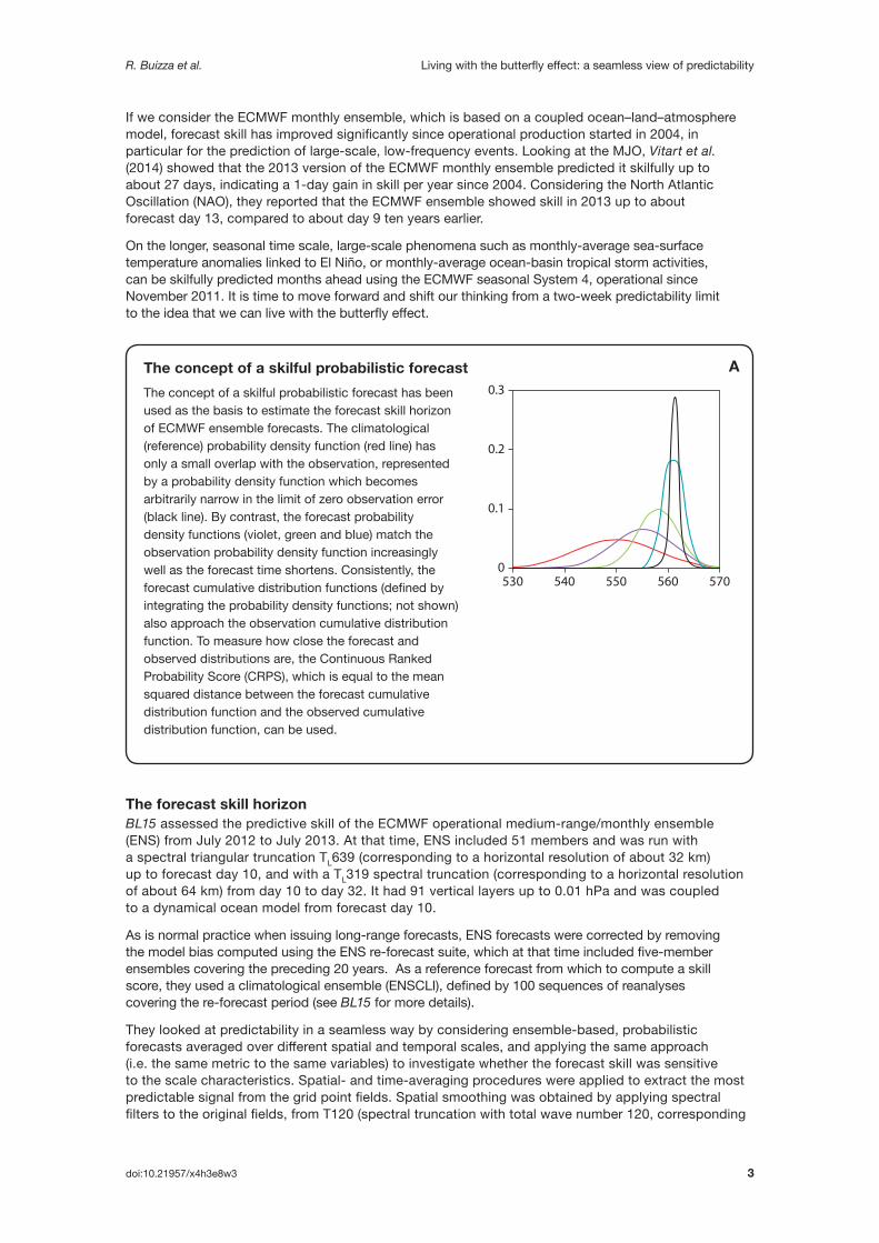
The concept of a skilful probabilistic forecastThe concept of a skilful probabilistic forecast has been used as the basis to estimate the forecast skill horizon of ECMWF ensemble forecasts. The climatological (reference) probability density function (red line) has only a small overlap with the observation, represented by a probability density function which becomes arbitrarily narrow in the limit of zero observation error (black line). By contrast, the forecast probability density functions (violet, green and blue) match the observation probability density function increasingly well as the forecast time shortens. Consistently, the forecast cumulative distribution functions (defined by integrating the probability density functions; not shown) also approach the observation cumulative distribution function. To measure how close the forecast and observed distributions are, the Continuous Ranked Probability Score (CRPS), which is equal to the mean squared distance between the forecast cumulative distribution function and the observed cumulative distribution function, can be used.

A0.3

0.2

0.1

0530 540 550 560 570

R. Buizza et al. Living with the butterfly effect: a seamless view of predictability

4 doi:10.21957/x4h3e8w3

to about 170 km horizontal grid spacing) to T7 (about 3,000 km horizontal grid spacing). Time-averaging was obtained by considering instantaneous fields, or to be more precise fields defined for a 40-minute period (i.e. twice the time step used in the numerical integration), and fields averaged over 1, 2, 4, 8 and 16 days.

BL15 defined the ‘forecast skill horizon’ as the lead time when the bias-corrected ensemble forecast ceased to be more skilful than the climatological distribution. More precisely, the forecast skill horizon was computed as the forecast time when the average CRPS of the bias-corrected ensemble stopped being statistically significantly lower, at the 99th-percentile level, than the CRPS of the climatological ensemble.

Sensitivity to spatial and temporal scalesFigure 1 shows the annual-average CRPS of the bias-corrected ensemble (ENSBC) and of the climatological forecasts (ENSCLI), and the skill score of ENSBC defined simply as the difference between the two, as follows:

Forecasts are for the 2-day time averages of 850 hPa temperature at T120 spectral truncation over the northern hemisphere (NH, points with latitude north of 30°N), the southern hemisphere (SH, points with latitude south of 30°S) and the tropics (TR, points with latitude between 20°S and 20°N), valid from 12 hours to 32 days, every 12 hours. The CRPSS confidence intervals hit the zero line at forecast day 25 for the northern hemisphere, at day 18 for the southern hemisphere and at day 26 for the tropics, indicating that the forecast skill horizon can be longer than two weeks.

Figure 2 shows the sensitivity of the forecast skill horizon to the temporal scale under consideration, for T120 spatial fields. It shows that time-averaging reduces not only the difference between the climatology and observations (measured by CRPS(ENSCLI)) but also the error growth rate (the rate at which the difference between the forecast and observations grows as lead times increase, measured by the slope of CRPS(ENSBC)). The net effect is that, as the time-averaging period is progressively extended from 40 minutes to 16 days, the forecast time when the two average CRPS curves intersect moves to larger values. If we consider, for example, the northern hemisphere (Figure 2a), the forecast skill horizon increases from 23 days for 40-minute average fields to 24.5 days for 1-day average fields, 25 days for 2-day average fields and more than 30 days for time-averaging periods of 4 days.

Results shown in Table 1 for 850 hPa temperature forecasts over the three regions (NH, SH and TR) indicate that the sensitivity to time-averaging is stronger than the sensitivity to spatial filtering. It is worth pointing out that the forecast skill horizon depends also on the geographic area, the season and the forecast field.

Generally speaking, these results indicate that larger spatial and temporal scales are more predictable by between 5 and 12 days than finer scales. They show that we should be more specific when we talk about the forecast skill horizon. The horizon is finite, but it is not the same for all scales, fields, areas and seasons.

Clearly, close to the forecast skill horizon the skill level is very small in absolute terms, and the number of users who can exploit this level of skill may be very limited. Nevertheless, our definition of the forecast skill horizon is objective, and, in line with general practice, defined by comparing the skill of a forecast with that of a well-defined unskilled reference forecast.

R. Buizza et al. Living with the butterfly effect: a seamless view of predictability

doi:10.21957/x4h3e8w3 5

Figure 2 Annual-average (107 cases) CRPS of the bias-corrected ensemble (ENSBC, solid lines) and the reference climatological ensemble (ENSCLI, dashed lines), for 850 hPa temperature fields with a T120 spectral truncation (about 170 km horizontal spacing) and with different degrees of time-averaging for (a) the northern hemisphere, (b) the southern hemisphere and (c) the tropics. Confidence intervals, which are essential to determine the forecast skill horizon, are not shown here for simplicity.

0

0.3

0.6

0.9

1.2

1.5

1.8CR

PS

Forecast day151050 20 25 30

Forecast day151050 20 25 30

Forecast day151050 20 25 30

Forecast day151050 20 25 30

Forecast day151050 20 25 30

Forecast day151050 20 25 30

00.20.40.60.8

11.21.41.6

CRPS

S

00.20.40.60.8

11.21.41.6

CRPS

0

0.2

0.4

0.6

0.8

1

1.2

CRPS

S

0

0.1

0.2

0.3

0.4

0.5

CRPS

0

0.1

0.2

CRPS

S

a Northern hemisphere

b Southern hemisphere

ClimatologyEnsembleforecasts

c Tropics

d Northern hemisphere – skill score

e Southern hemisphere – skill score

f Tropics – skill score

0

1

2

0

1

2

00.10.20.30.40.50.60.7 40-minute average

1-day average2-day average4-day average8-day average16-day average

Dashed lines = climatologySolid lines = ensemble forecasts

CRPS

Forecast day151050 20 25 30

Forecast day151050 20 25 30

Forecast day151050 20 25 30

CRPS

CRPS

a Northern hemisphere b Southern hemisphere

c Tropics

Figure 1 CRPS of the bias-corrected ensemble (ENSBC) and the reference climatological ensemble (ENSCLI) for 850 hPa temperature fields, for a 2-day time average and a T120 spectral truncation (about 170 km horizontal spacing) for (a) the northern hemisphere, (b) the southern hemisphere and (c) the tropics; and the CRPSS(ENSBC) (see text for definition) with 98thpercentile confidence internals for (d) the northern hemisphere, (e) the southern hemisphere and (f) the tropics.

R. Buizza et al. Living with the butterfly effect: a seamless view of predictability

6 doi:10.21957/x4h3e8w3

Implications for forecastersThe results presented here show that ECMWF bias-corrected ensemble forecasts over a wide range of spatial and temporal scales can have forecast skill horizons longer than the two weeks estimated by Lorenz (1969a, b). This result is not new: it confirms results published over the last 20 years (e.g. Shukla, 1998) that were obtained by applying different methodologies and metrics and looking at some specific phenomena, such as the MJO, the NAO and El Niño. What is new in this work is that the forecast skill horizon has been measured in a seamless way for forecasts with different spatial and temporal scales, by applying the same metric from day 0 to forecast day 32.

These results have clear implications for forecasters: large-scale features, such as the presence of blocking conditions over the Euro-Atlantic sector, can be predicted with some skill three to four weeks ahead. This means that forecasters can look at long-range forecasts of large-scale, time-average features to detect whether, for example, the weekly-average temperature distribution at the surface is shifted towards warmer or colder conditions. But at this forecast range they cannot expect to extract finer details, such as what the temperature at a specific location will be. They will have to wait until the forecast range is, for example, only a few days to be able to skilfully predict these finer details, such as the temperature on a specific day and at a precise location. In other words, as the forecast lead time shortens, the forecaster can zoom in on details at increasingly finer spatial and temporal scales.

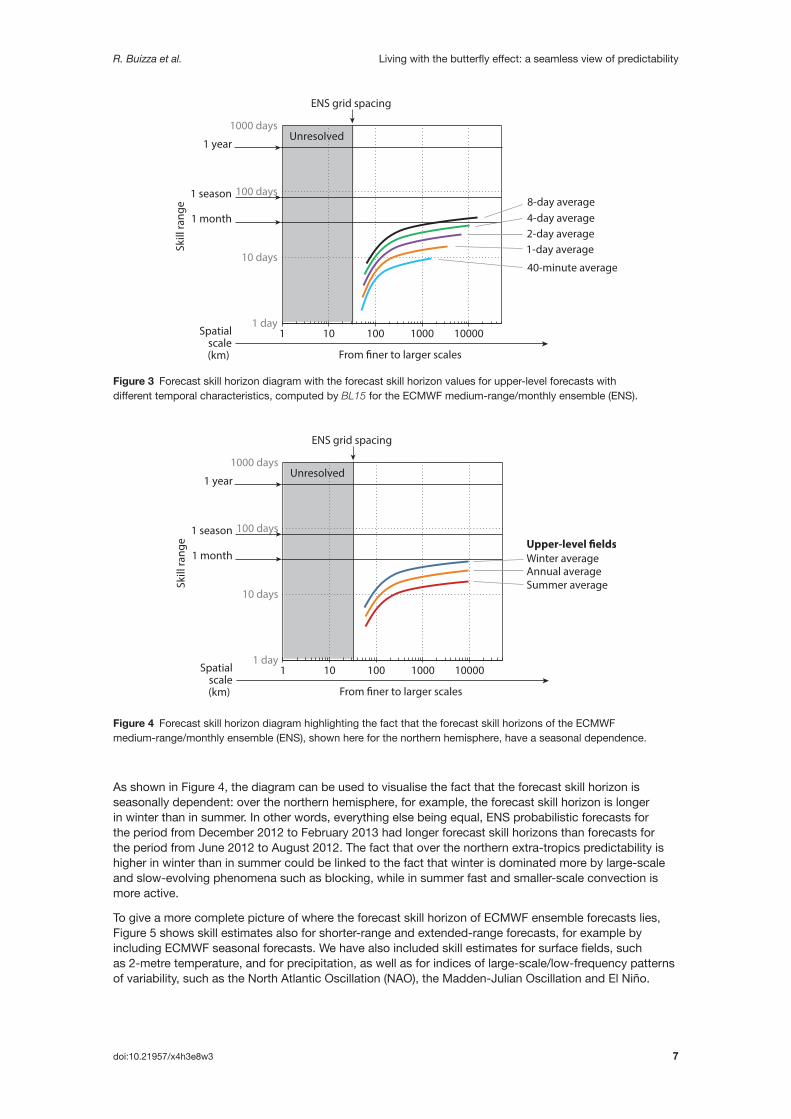
Visualising the forecast skill horizon Figure 3 introduces the forecast skill horizon diagram, which can be used to visualise seamlessly the fact that predictive skill depends on the spatial and temporal scales of forecast phenomena. In the diagram, the x-axis is the horizontal spatial scale of predicted aspects of the weather (in km), and the y-axis is the forecast skill range, in days. The grey rectangle to the left of x = 32 km identifies the scales that are definitely unresolved in the ECMWF ENS, which today has a grid spacing of about 32 km. It should be noted that the effective resolution, in the sense of the ability to represent a weather feature adequately, can be lower than the grid spacing by a factor of five or more.

In Figure 3, the forecast horizon skill diagram is applied to the ECMWF medium-range/monthly ensemble (ENS) forecasts studied in BL15. Each coloured line illustrates how the forecast skill horizon varies with the spatial scale after time averaging has been applied (from the most detailed, 40-minute to the 8-day time-average). Each line represents an average forecast skill horizon, computed considering seven upper-air variables (geopotential height at 500 hPa, temperature and wind components at 850 and 200 hPa) and three areas (NH, SH and TR). The 8-day average line is positioned higher in the vertical than the 40-minute line, reflecting the fact that time-averaged fields are more predictable than instantaneous fields. The lines for the other time-average periods (1, 2 and 4 days) lie between these two.

Temperature 850 hPa

40-minute average 2-day average 8-day average

NH SH TR NH SH TR NH SH TR

T120(170 km) 23.0 16.5 22.0 25.0 18.0 26.0 > 28.0 25.0 > 28.0

T30(680 km) 24.0 17.0 23.0 25.0 18.0 27.0 > 28.0 25.5 > 28.0

T7(3,000 km) > 32.0 23.0 26.5 > 31.0 23.5 28.0 > 28.0 > 28.0 > 28.0

Table 1 Forecast skill horizons for the probabilistic prediction of 850 hPa temperature over the northern hemisphere (NH), the southern hemisphere (SH) and the tropics (TR), for fields with increasingly larger spatial scales (T120, T30 and T7 spectral triangular truncation) and longer time averages (40-minute, 2-day and 8-day averages). The ‘greater than’ symbol (>) indicates that the forecast skill horizon is larger than the last time step that could be verified (i.e. 32 days for 40-minute average forecasts, 31 days for 2-day average forecasts and 28 days for 8-day average forecasts).

R. Buizza et al. Living with the butterfly effect: a seamless view of predictability

doi:10.21957/x4h3e8w3 7

As shown in Figure 4, the diagram can be used to visualise the fact that the forecast skill horizon is seasonally dependent: over the northern hemisphere, for example, the forecast skill horizon is longer in winter than in summer. In other words, everything else being equal, ENS probabilistic forecasts for the period from December 2012 to February 2013 had longer forecast skill horizons than forecasts for the period from June 2012 to August 2012. The fact that over the northern extra-tropics predictability is higher in winter than in summer could be linked to the fact that winter is dominated more by large-scale and slow-evolving phenomena such as blocking, while in summer fast and smaller-scale convection is more active.

To give a more complete picture of where the forecast skill horizon of ECMWF ensemble forecasts lies, Figure 5 shows skill estimates also for shorter-range and extended-range forecasts, for example by including ECMWF seasonal forecasts. We have also included skill estimates for surface fields, such as 2-metre temperature, and for precipitation, as well as for indices of large-scale/low-frequency patterns of variability, such as the North Atlantic Oscillation (NAO), the Madden-Julian Oscillation and El Niño.

Figure 3 Forecast skill horizon diagram with the forecast skill horizon values for upper-level forecasts with different temporal characteristics, computed by BL15 for the ECMWF medium-range/monthly ensemble (ENS).

Figure 4 Forecast skill horizon diagram highlighting the fact that the forecast skill horizons of the ECMWF medium-range/monthly ensemble (ENS), shown here for the northern hemisphere, have a seasonal dependence.

1 day

10 days

100 days

1000 days

1 10 100 1000 10000

Skill

rang

e

Spatialscale(km)

1 year

1 season

1 month

From �ner to larger scales

ENS grid spacing

Unresolved

8-day average4-day average2-day average1-day average

40-minute average

1 day

10 days

100 days

1000 days

1 10 100 1000 10000

Skill

rang

e

Spatialscale(km)

1 year

1 season

1 month

From �ner to larger scales

ENS grid spacing

Unresolved

Upper-level fieldsWinter averageAnnual averageSummer average

R. Buizza et al. Living with the butterfly effect: a seamless view of predictability

8 doi:10.21957/x4h3e8w3

Figure 5 visualizes the forecast skill horizon considering all these fields. The red lines relating to the instantaneous and finer-scale surface variables are closer to the x-axis, illustrating the fact that surface variables are less predictable. By contrast, the blue lines relating to large-scale patterns identified by teleconnection indices (e.g. NAO and MJO) and to the average sea-surface temperature (SST) in the Pacific regions affected by El Niño are further away from the x-axis and closer to the top-right part of the diagram. This illustrates the fact that these large-scale patterns can be skilfully predicted months ahead.

Two further features have been added to the diagram: a blue-line envelope, drawn schematically to include all the individual lines, and a red ‘no-skill’ region. The blue line shows where the forecast skill horizon for the ECMWF ensemble forecast is today: relatively short, less than 10 days, for very detailed forecasts, but transitioning to very long horizons of up to a year for monthly-average SST forecasts for regions in the tropical Pacific. The blue line is not straight, parallel to the x-axis and with a value of about two weeks, as it would be if there were a fixed limit to predictability, but it is curved, reflecting the fact that the forecast skill horizon is scale-dependent, variable-dependent, area-dependent, and season-dependent.

The forecast skill horizon challengeThe forecast skill diagram, built with a seamless approach to fields with different spatial and temporal characteristics, visualises our understanding of the predictability of different scales of atmospheric variability. It illustrates the fact that, thanks to scientific and model advances, a better estimation of initial conditions using more and better observations and more accurate assimilation methods, and the use of ensemble methods, we can extract predictable signals from the larger scales, notwithstanding the upscale error propagation from the small scales.

The interplay between the downscale propagation of predictability and the upscale error propagation – the battle between the sources and sinks of predictive skill – determines where the forecast skill horizon lies.

By further improving our ensembles, increasing the resolution of the models, reducing the initial error, and adding a better and more complete description of all relevant phenomena, we can aim to further push this line towards the top-left corner. In other words, we can live with the butterfly effect and further extend the forecast skill horizon.

Figure 5 The forecast skill horizon of ECMWF operational forecasts, constructed using published skill measures of medium-range/monthly (ENS) and seasonal (S4) forecasts.

1 day

10 days

100 days

1000 days

1 10 100 1000 10000

Skill

rang

e

Spatialscale(km)

1 year

1 season

1 month

From �ner to larger scales

ENS grid spacing

Unresolved No skill Monthly average sea-surface temperature (e.g. El Niño)

Teleconnection indices

Monthly average2-metre temperature, mean sea level pressure

Upper-level �elds

Surface �elds Rainfall Extremes

R. Buizza et al. Living with the butterfly effect: a seamless view of predictability

doi:10.21957/x4h3e8w3 9

Further readingBechtold, P., P. Bauer, P. Berrisford, J. Bidlot, C. Cardinali, T. Haiden, M. Janousek, D. Klocke, L. Magnusson, A. McNally, F. Prates, M. Rodwell, N. Semane, F. Vitart, 2012: Progress in predicting tropical systems: The role of convection. ECMWF Research Department Technical Memorandum no. 686.

Buizza, R., & Leutbecher, M., 2015: The Forecast Skill Horizon. ECMWF Research Department Technical Memorandum no. 754. Also Q. J. Roy. Meteorol. Soc., in press.

Hoskins, B. J., 2013: Review article: the potential for skill across the range of the seamless weather-climate prediction problem: a stimulus for our science. Q. J. R. Meteorol. Soc., 139, 573–584.

Lorenz, E. N., 1969a: The predictability of a flow which possesses many scales of motion. Tellus, XXI, 3, 289–307.

Lorenz, E. N., 1969b: How much better can weather prediction become? Technology Review, July/August, 39–49.

Shukla, J., 1998: Predictability in the midst of chaos: a scientific basis for climate forecasting. J. Atmos. Sci., 38, 2547–2572.

Vitart, F., G. Balsamo, R. Buizza, L. Ferranti, S. Keeley, L. Magnusson, F. Molteni, & A. Weisheimer, 2014: Sub-seasonal predictions. ECMWF Research Department Technical Memorandum no. 734

© Copyright 2016

European Centre for Medium-Range Weather Forecasts, Shinfield Park, Reading, RG2 9AX, England

The content of this Newsletter article is available for use under a Creative Commons Attribution-Non-Commercial- No-Derivatives-4.0-Unported Licence. See the terms at https://creativecommons.org/licenses/by-nc-nd/4.0/.

The information within this publication is given in good faith and considered to be true, but ECMWF accepts no liability for error or omission or for loss or damage arising from its use.