Linear System Theory Control Matrix Computations
156
Summer Course Linear System Theory Control & Matrix Computations Monopoli September 8–12, 2008
Transcript of Linear System Theory Control Matrix Computations
Summer Course
Linear System TheoryControl
&Matrix Computations
Monopoli September 8–12, 2008
Lecture 2: Linear differential systems
Lecturer: Paolo Rapisarda

Part I: Representations
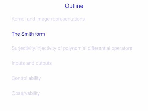
Outline
Kernel and image representations
The Smith form
Surjectivity/injectivity of polynomial differential operators
Inputs and outputs
Controllability
Observability
Definition
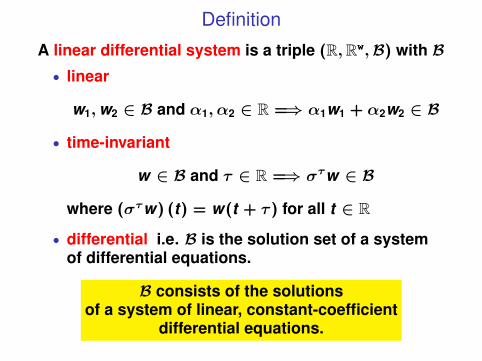
A linear differential system is a triple (R,Rw,B) with B• linear
w1,w2 ∈ B and α1, α2 ∈ R =⇒ α1w1 + α2w2 ∈ B
• time-invariant
w ∈ B and τ ∈ R =⇒ στw ∈ B
where (στw) (t) = w(t + τ ) for all t ∈ R
• differential i.e. B is the solution set of a systemof differential equations.
B consists of the solutionsof a system of linear, constant-coefficient
differential equations.
Definition
A linear differential system is a triple (R,Rw,B) with B• linear
w1,w2 ∈ B and α1, α2 ∈ R =⇒ α1w1 + α2w2 ∈ B
• time-invariant
w ∈ B and τ ∈ R =⇒ στw ∈ B
where (στw) (t) = w(t + τ ) for all t ∈ R
• differential i.e. B is the solution set of a systemof differential equations.
B consists of the solutionsof a system of linear, constant-coefficient
differential equations.
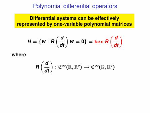
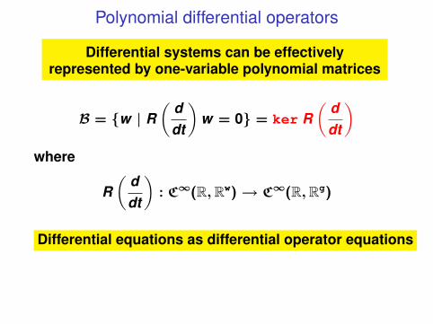
Polynomial differential operators
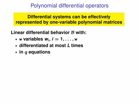
Differential systems can be effectivelyrepresented by one-variable polynomial matrices
Polynomial differential operators
Differential systems can be effectivelyrepresented by one-variable polynomial matrices
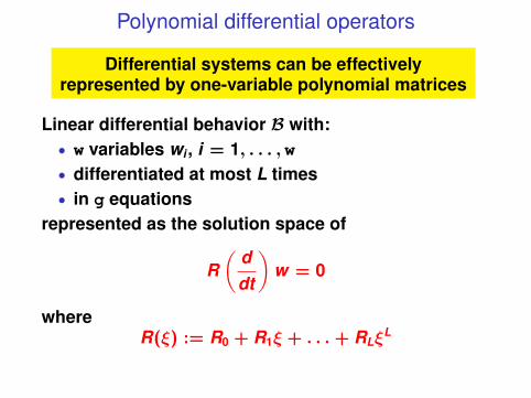
Linear differential behavior B with:• w variables wi , i = 1, . . . , w• differentiated at most L times• in g equations
Polynomial differential operators
Differential systems can be effectivelyrepresented by one-variable polynomial matrices
Linear differential behavior B with:• w variables wi , i = 1, . . . , w• differentiated at most L times• in g equations
represented as the solution space of
R(
ddt
)w = 0
whereR(ξ) := R0 + R1ξ + . . . + RLξ
L
Polynomial differential operators
Differential systems can be effectivelyrepresented by one-variable polynomial matrices
B = {w | R(
ddt
)w = 0} = ker R
(ddt
)where
R(
ddt
): C∞(R,Rw)→ C∞(R,Rg)
Polynomial differential operators
Differential systems can be effectivelyrepresented by one-variable polynomial matrices
B = {w | R(
ddt
)w = 0} = ker R
(ddt
)where
R(
ddt
): C∞(R,Rw)→ C∞(R,Rg)
Differential equations as differential operator equations
Outline
Kernel and image representations
The Smith form
Surjectivity/injectivity of polynomial differential operators
Inputs and outputs
Controllability
Observability
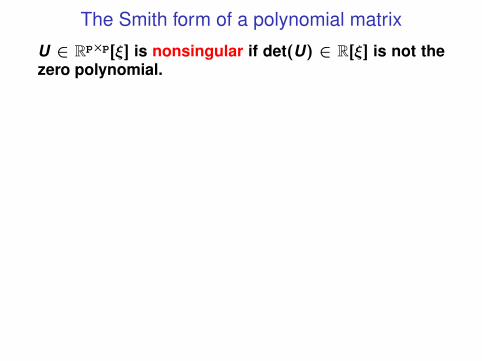
The Smith form of a polynomial matrix
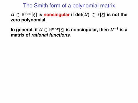
U ∈ Rp×p[ξ] is nonsingular if det(U) ∈ R[ξ] is not thezero polynomial.
The Smith form of a polynomial matrix
U ∈ Rp×p[ξ] is nonsingular if det(U) ∈ R[ξ] is not thezero polynomial.
In general, if U ∈ Rp×p[ξ] is nonsingular, then U−1 is amatrix of rational functions.
The Smith form of a polynomial matrix
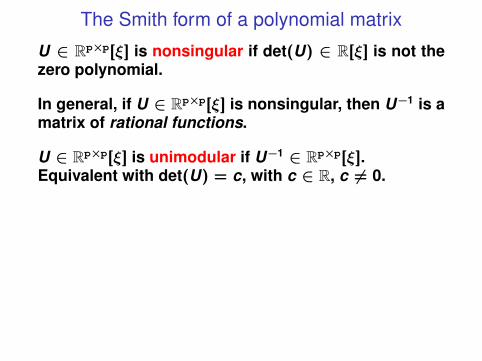
U ∈ Rp×p[ξ] is nonsingular if det(U) ∈ R[ξ] is not thezero polynomial.
In general, if U ∈ Rp×p[ξ] is nonsingular, then U−1 is amatrix of rational functions.
U ∈ Rp×p[ξ] is unimodular if U−1 ∈ Rp×p[ξ].Equivalent with det(U) = c, with c ∈ R, c 6= 0.
The Smith form of a polynomial matrix
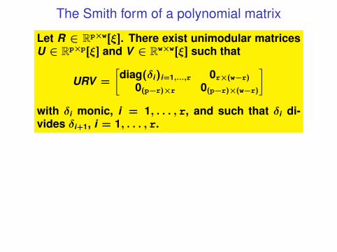
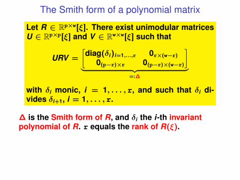
Let R ∈ Rp×w[ξ]. There exist unimodular matricesU ∈ Rp×p[ξ] and V ∈ Rw×w[ξ] such that
URV =
[diag(δi)i=1,...,r 0r×(w−r)
0(p−r)×r 0(p−r)×(w−r)
]with δi monic, i = 1, . . . , r, and such that δi di-vides δi+1, i = 1, . . . , r.
The Smith form of a polynomial matrix
The Smith form of a polynomial matrix
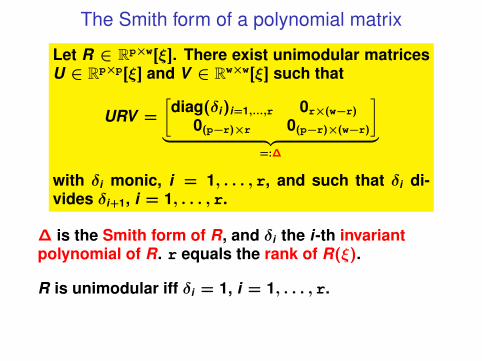
Let R ∈ Rp×w[ξ]. There exist unimodular matricesU ∈ Rp×p[ξ] and V ∈ Rw×w[ξ] such that
URV =
[diag(δi)i=1,...,r 0r×(w−r)
0(p−r)×r 0(p−r)×(w−r)
]︸ ︷︷ ︸
=:∆
with δi monic, i = 1, . . . , r, and such that δi di-vides δi+1, i = 1, . . . , r.
∆ is the Smith form of R, and δi the i-th invariantpolynomial of R. r equals the rank of R(ξ).
The Smith form of a polynomial matrix
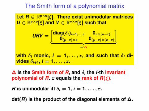
Let R ∈ Rp×w[ξ]. There exist unimodular matricesU ∈ Rp×p[ξ] and V ∈ Rw×w[ξ] such that
URV =
[diag(δi)i=1,...,r 0r×(w−r)
0(p−r)×r 0(p−r)×(w−r)
]︸ ︷︷ ︸
=:∆
with δi monic, i = 1, . . . , r, and such that δi di-vides δi+1, i = 1, . . . , r.
∆ is the Smith form of R, and δi the i-th invariantpolynomial of R. r equals the rank of R(ξ).
R is unimodular iff δi = 1, i = 1, . . . , r.
The Smith form of a polynomial matrix
Let R ∈ Rp×w[ξ]. There exist unimodular matricesU ∈ Rp×p[ξ] and V ∈ Rw×w[ξ] such that
URV =
[diag(δi)i=1,...,r 0r×(w−r)
0(p−r)×r 0(p−r)×(w−r)
]︸ ︷︷ ︸
=:∆
with δi monic, i = 1, . . . , r, and such that δi di-vides δi+1, i = 1, . . . , r.
∆ is the Smith form of R, and δi the i-th invariantpolynomial of R. r equals the rank of R(ξ).
R is unimodular iff δi = 1, i = 1, . . . , r.
det(R) is the product of the diagonal elements of ∆.
Outline
Kernel and image representations
The Smith form
Surjectivity/injectivity of polynomial differential operators
Inputs and outputs
Controllability
Observability
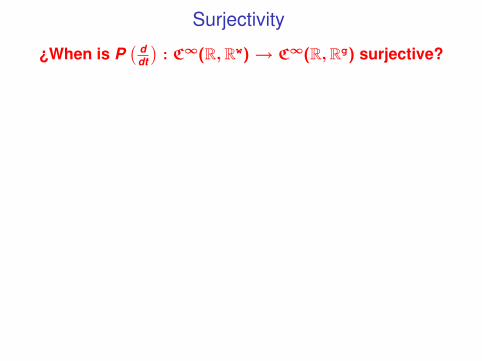
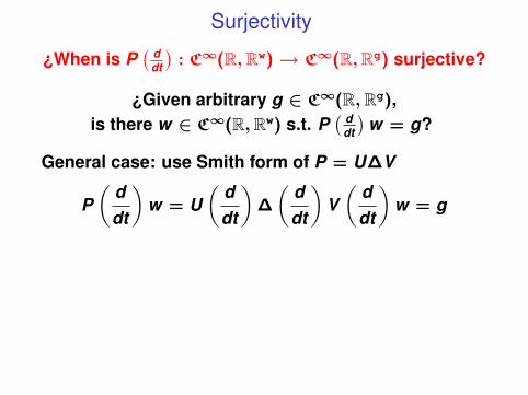
Surjectivity
¿When is P( d
dt
): C∞(R,Rw)→ C∞(R,Rg) surjective?
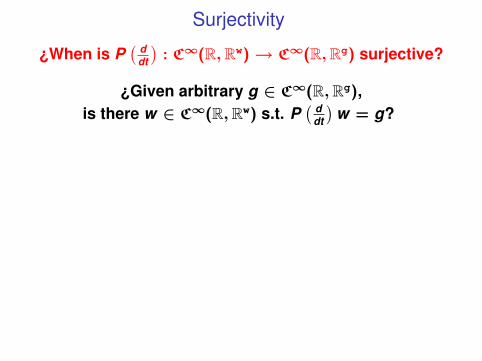
Surjectivity
¿When is P( d
dt
): C∞(R,Rw)→ C∞(R,Rg) surjective?
¿Given arbitrary g ∈ C∞(R,Rg),is there w ∈ C∞(R,Rw) s.t. P
( ddt
)w = g?
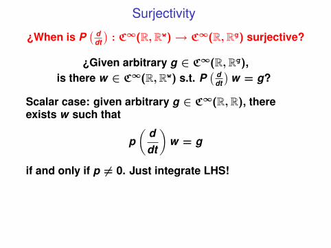
Surjectivity
¿When is P( d
dt
): C∞(R,Rw)→ C∞(R,Rg) surjective?
¿Given arbitrary g ∈ C∞(R,Rg),is there w ∈ C∞(R,Rw) s.t. P
( ddt
)w = g?
Scalar case: given arbitrary g ∈ C∞(R,R), thereexists w such that
p(
ddt
)w = g
if and only if p 6= 0. Just integrate LHS!
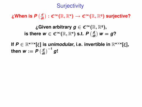
Surjectivity
¿When is P( d
dt
): C∞(R,Rw)→ C∞(R,Rg) surjective?
¿Given arbitrary g ∈ C∞(R,Rg),is there w ∈ C∞(R,Rw) s.t. P
( ddt
)w = g?
If P ∈ Rw×w[ξ] is unimodular, i.e. invertible in Rw×w[ξ],then w := P
( ddt
)−1g!
Surjectivity
¿When is P( d
dt
): C∞(R,Rw)→ C∞(R,Rg) surjective?
¿Given arbitrary g ∈ C∞(R,Rg),is there w ∈ C∞(R,Rw) s.t. P
( ddt
)w = g?
General case: use Smith form of P = U∆V
P(
ddt
)w = U
(ddt
)∆
(ddt
)V(
ddt
)w = g
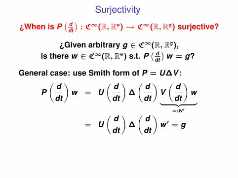
Surjectivity
¿When is P( d
dt
): C∞(R,Rw)→ C∞(R,Rg) surjective?
¿Given arbitrary g ∈ C∞(R,Rg),is there w ∈ C∞(R,Rw) s.t. P
( ddt
)w = g?
General case: use Smith form of P = U∆V :
P(
ddt
)w = U
(ddt
)∆
(ddt
)V(
ddt
)w︸ ︷︷ ︸
=:w ′
= U(
ddt
)∆
(ddt
)w ′ = g
Surjectivity
¿When is P( d
dt
): C∞(R,Rw)→ C∞(R,Rg) surjective?
¿Given arbitrary g ∈ C∞(R,Rg),is there w ∈ C∞(R,Rw) s.t. P
( ddt
)w = g?
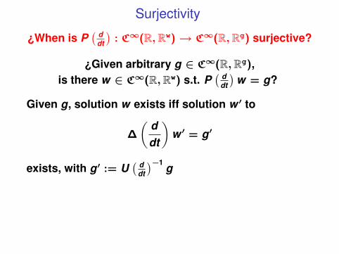
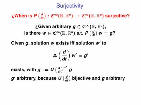
Given g, solution w exists iff solution w ′ to
∆
(ddt
)w ′ = g′
exists, with g′ := U( d
dt
)−1g
Surjectivity
¿When is P( d
dt
): C∞(R,Rw)→ C∞(R,Rg) surjective?
¿Given arbitrary g ∈ C∞(R,Rg),is there w ∈ C∞(R,Rw) s.t. P
( ddt
)w = g?
Given g, solution w exists iff solution w ′ to
∆
(ddt
)w ′ = g′
exists, with g′ := U( d
dt
)−1g
g′ arbitrary, because U( d
dt
)bijective and g arbitrary
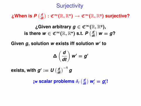
Surjectivity
¿When is P( d
dt
): C∞(R,Rw)→ C∞(R,Rg) surjective?
¿Given arbitrary g ∈ C∞(R,Rg),is there w ∈ C∞(R,Rw) s.t. P
( ddt
)w = g?
Given g, solution w exists iff solution w ′ to
∆
(ddt
)w ′ = g′
exists, with g′ := U( d
dt
)−1g
¡w scalar problems δi( d
dt
)w ′i = g′i !
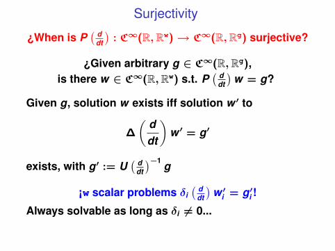
Surjectivity
¿When is P( d
dt
): C∞(R,Rw)→ C∞(R,Rg) surjective?
¿Given arbitrary g ∈ C∞(R,Rg),is there w ∈ C∞(R,Rw) s.t. P
( ddt
)w = g?
Given g, solution w exists iff solution w ′ to
∆
(ddt
)w ′ = g′
exists, with g′ := U( d
dt
)−1g
¡w scalar problems δi( d
dt
)w ′i = g′i !
Always solvable as long as δi 6= 0...
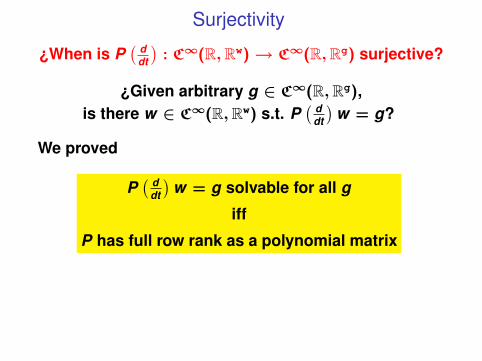
Surjectivity
¿When is P( d
dt
): C∞(R,Rw)→ C∞(R,Rg) surjective?
¿Given arbitrary g ∈ C∞(R,Rg),is there w ∈ C∞(R,Rw) s.t. P
( ddt
)w = g?
We proved
P( d
dt
)w = g solvable for all g
iff
P has full row rank as a polynomial matrix
Injectivity
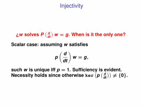
¿w solves P( d
dt
)w = g. When is it the only one?
Injectivity
¿w solves P( d
dt
)w = g. When is it the only one?
Scalar case: assuming w satisfies
p(
ddt
)w = g,
such w is unique iff p = 1. Sufficiency is evident.Necessity holds since otherwise ker
(p( d
dt
))6= {0}.

Injectivity
¿w solves P( d
dt
)w = g. When is it the only one?
General case: Use Smith form of P = U∆V to write
∆
(ddt
)w ′ = g′
with w ′ := V( d
dt
)w , g′ := U
( ddt
)−1g
Injectivity
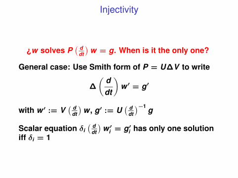
¿w solves P( d
dt
)w = g. When is it the only one?
General case: Use Smith form of P = U∆V to write
∆
(ddt
)w ′ = g′
with w ′ := V( d
dt
)w , g′ := U
( ddt
)−1g
Scalar equation δi( d
dt
)w ′i = g′i has only one solution
iff δi = 1
Injectivity
¿w solves P( d
dt
)w = g. When is it the only one?
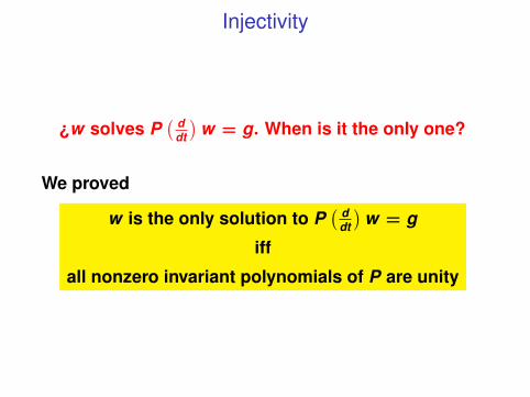
We proved
w is the only solution to P( d
dt
)w = g
iff
all nonzero invariant polynomials of P are unity
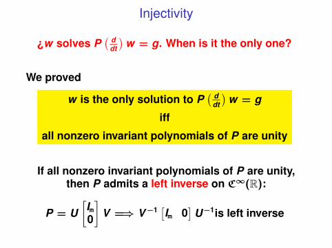
Injectivity
¿w solves P( d
dt
)w = g. When is it the only one?
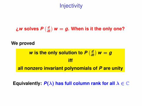
We proved
w is the only solution to P( d
dt
)w = g
iff
all nonzero invariant polynomials of P are unity
Equivalently: P(λ) has full column rank for all λ ∈ C
Injectivity
¿w solves P( d
dt
)w = g. When is it the only one?
We proved
w is the only solution to P( d
dt
)w = g
iff
all nonzero invariant polynomials of P are unity
If all nonzero invariant polynomials of P are unity,then P admits a left inverse on C∞(R):
P = U[Im0
]V =⇒ V−1 [Im 0
]U−1is left inverse
Summary
• Polynomial differential operator equations;
• Surjectivity: P full row rank over R•×•[ ξ], as apolynomial matrix
• Injectivity: P(λ) full column rank for all λ ∈ C, asa matrix over R•×•
Summary
• Polynomial differential operator equations;
• Surjectivity: P full row rank over R•×•[ ξ], as apolynomial matrix
• Injectivity: P(λ) full column rank for all λ ∈ C, asa matrix over R•×•
Summary
• Polynomial differential operator equations;
• Surjectivity: P full row rank over R•×•[ ξ], as apolynomial matrix
• Injectivity: P(λ) full column rank for all λ ∈ C, asa matrix over R•×•
Outline
Kernel and image representations
The Smith form
Surjectivity/injectivity of polynomial differential operators
Inputs and outputs
Controllability
Observability
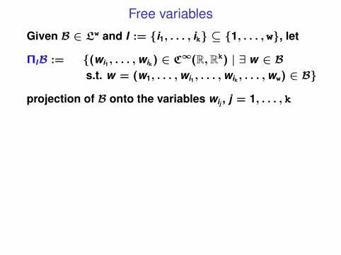
Free variables
Given B ∈ Lw and I := {i1, . . . , ik} ⊆ {1, . . . , w}, let
ΠIB := {(wi1, . . . ,wik) ∈ C∞(R,Rk) | ∃ w ∈ Bs.t. w = (w1, . . . ,wi1, . . . ,wik, . . . ,ww) ∈ B}
projection of B onto the variables wij , j = 1, . . . , k
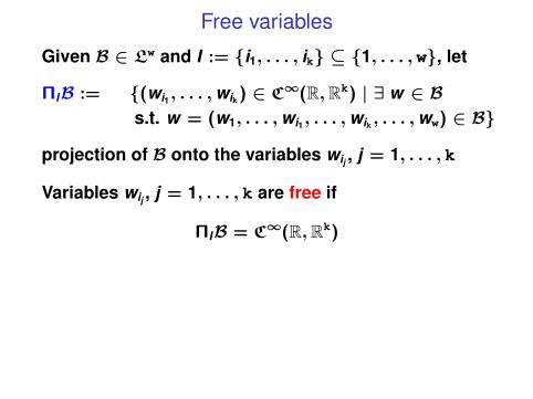
Free variables
Given B ∈ Lw and I := {i1, . . . , ik} ⊆ {1, . . . , w}, let
ΠIB := {(wi1, . . . ,wik) ∈ C∞(R,Rk) | ∃ w ∈ Bs.t. w = (w1, . . . ,wi1, . . . ,wik, . . . ,ww) ∈ B}
projection of B onto the variables wij , j = 1, . . . , k
Variables wij , j = 1, . . . , k are free if
ΠIB = C∞(R,Rk)
Free variables
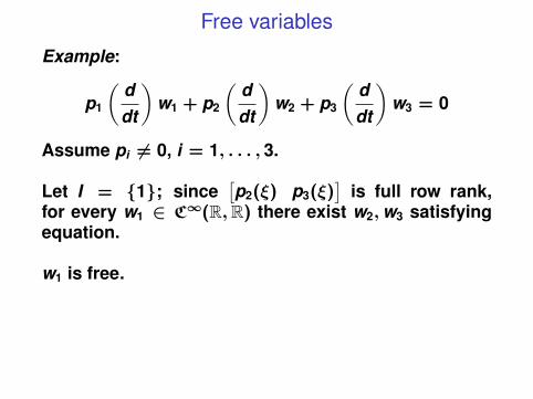
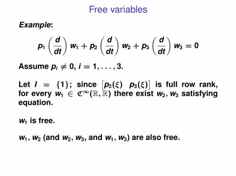
Example:
p1
(ddt
)w1 + p2
(ddt
)w2 + p3
(ddt
)w3 = 0
Assume pi 6= 0, i = 1, . . . , 3.
Let I = {1}; since[p2(ξ) p3(ξ)
]is full row rank,
for every w1 ∈ C∞(R,R) there exist w2,w3 satisfyingequation.
w1 is free.
Free variables
Example:
p1
(ddt
)w1 + p2
(ddt
)w2 + p3
(ddt
)w3 = 0
Assume pi 6= 0, i = 1, . . . , 3.
Let I = {1}; since[p2(ξ) p3(ξ)
]is full row rank,
for every w1 ∈ C∞(R,R) there exist w2,w3 satisfyingequation.
w1 is free.
w1,w2 (and w2,w3, and w1,w3) are also free.
Maximally free sets
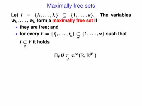
Let I = {i1, . . . , ik} ⊆ {1, . . . , w}. The variableswi1, . . . ,wik form a maximally free set if
• they are free; and• for every I ′ = {i ′1, . . . , i ′k} ⊂6=
{1, . . . , w} such that
I ⊂6=
I ′ it holds
ΠI′B ⊂6=
C∞(R,R|I′|)
Maximally free sets
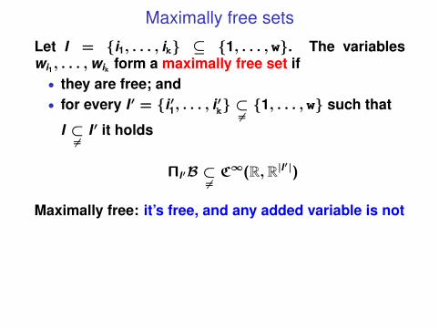
Let I = {i1, . . . , ik} ⊆ {1, . . . , w}. The variableswi1, . . . ,wik form a maximally free set if
• they are free; and• for every I ′ = {i ′1, . . . , i ′k} ⊂6=
{1, . . . , w} such that
I ⊂6=
I ′ it holds
ΠI′B ⊂6=
C∞(R,R|I′|)
Maximally free: it’s free, and any added variable is not
Maximally free sets
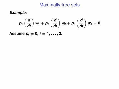
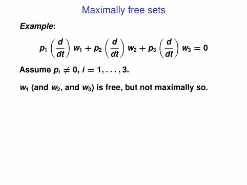
Example:
p1
(ddt
)w1 + p2
(ddt
)w2 + p3
(ddt
)w3 = 0
Assume pi 6= 0, i = 1, . . . , 3.
Maximally free sets
Example:
p1
(ddt
)w1 + p2
(ddt
)w2 + p3
(ddt
)w3 = 0
Assume pi 6= 0, i = 1, . . . , 3.
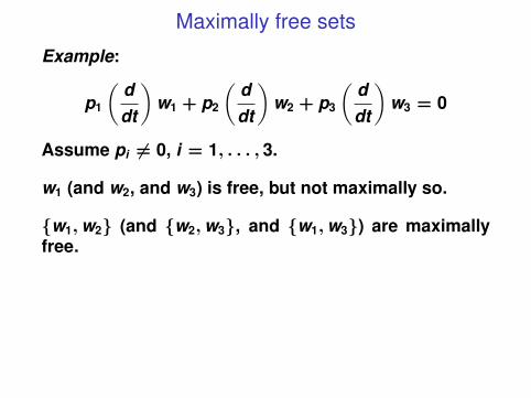
w1 (and w2, and w3) is free, but not maximally so.
Maximally free sets
Example:
p1
(ddt
)w1 + p2
(ddt
)w2 + p3
(ddt
)w3 = 0
Assume pi 6= 0, i = 1, . . . , 3.
w1 (and w2, and w3) is free, but not maximally so.
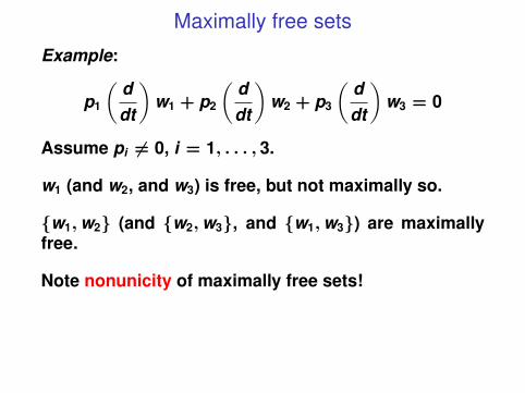
{w1,w2} (and {w2,w3}, and {w1,w3}) are maximallyfree.
Maximally free sets
Example:
p1
(ddt
)w1 + p2
(ddt
)w2 + p3
(ddt
)w3 = 0
Assume pi 6= 0, i = 1, . . . , 3.
w1 (and w2, and w3) is free, but not maximally so.
{w1,w2} (and {w2,w3}, and {w1,w3}) are maximallyfree.
Note nonunicity of maximally free sets!
Inputs and outputs
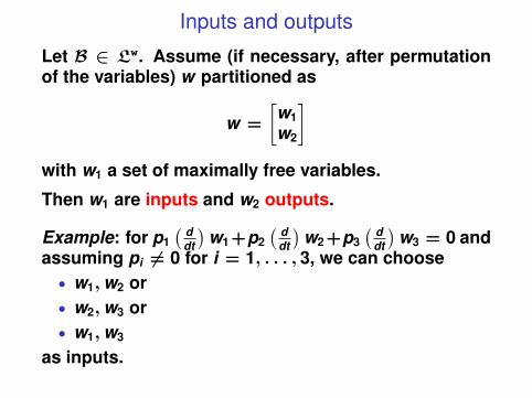
Let B ∈ Lw. Assume (if necessary, after permutationof the variables) w partitioned as
w =
[w1w2
]with w1 a set of maximally free variables.
Then w1 are inputs and w2 outputs.
Inputs and outputs
Let B ∈ Lw. Assume (if necessary, after permutationof the variables) w partitioned as
w =
[w1w2
]with w1 a set of maximally free variables.
Then w1 are inputs and w2 outputs.
Example: for p1( d
dt
)w1 +p2
( ddt
)w2 +p3
( ddt
)w3 = 0 and
assuming pi 6= 0 for i = 1, . . . , 3, we can choose• w1,w2 or• w2,w3 or• w1,w3
as inputs.
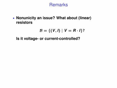
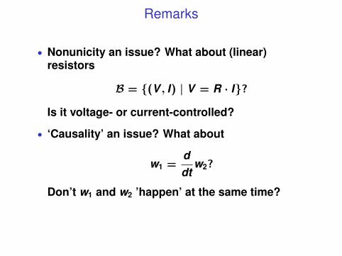
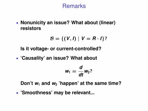
Remarks
• Nonunicity an issue? What about (linear)resistors
B = {(V , I) | V = R · I}?
Is it voltage- or current-controlled?
• ‘Causality’ an issue? What about
w1 =ddt
w2?
Don’t w1 and w2 ’happen’ at the same time?
• ’Smoothness’ may be relevant...
Remarks
• Nonunicity an issue? What about (linear)resistors
B = {(V , I) | V = R · I}?
Is it voltage- or current-controlled?
• ‘Causality’ an issue? What about
w1 =ddt
w2?
Don’t w1 and w2 ’happen’ at the same time?
• ’Smoothness’ may be relevant...
Remarks
• Nonunicity an issue? What about (linear)resistors
B = {(V , I) | V = R · I}?
Is it voltage- or current-controlled?
• ‘Causality’ an issue? What about
w1 =ddt
w2?
Don’t w1 and w2 ’happen’ at the same time?
• ’Smoothness’ may be relevant...
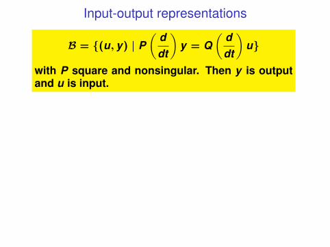
Input-output representations
B = {(u, y) | P(
ddt
)y = Q
(ddt
)u}
with P square and nonsingular. Then y is outputand u is input.
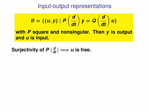
Input-output representations
B = {(u, y) | P(
ddt
)y = Q
(ddt
)u}
with P square and nonsingular. Then y is outputand u is input.
Surjectivity of P( d
dt
)=⇒ u is free.
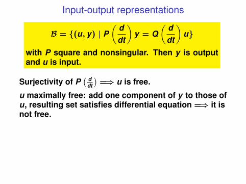
Input-output representations
B = {(u, y) | P(
ddt
)y = Q
(ddt
)u}
with P square and nonsingular. Then y is outputand u is input.
Surjectivity of P( d
dt
)=⇒ u is free.
u maximally free: add one component of y to those ofu, resulting set satisfies differential equation =⇒ it isnot free.
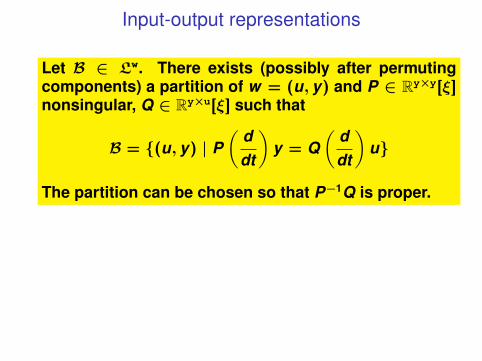
Input-output representations
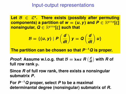
Let B ∈ Lw. There exists (possibly after permutingcomponents) a partition of w = (u, y) and P ∈ Ry×y[ξ]nonsingular, Q ∈ Ry×u[ξ] such that
B = {(u, y) | P(
ddt
)y = Q
(ddt
)u}
The partition can be chosen so that P−1Q is proper.
Input-output representations
Let B ∈ Lw. There exists (possibly after permutingcomponents) a partition of w = (u, y) and P ∈ Ry×y[ξ]nonsingular, Q ∈ Ry×u[ξ] such that
B = {(u, y) | P(
ddt
)y = Q
(ddt
)u}
The partition can be chosen so that P−1Q is proper.
Proof: Assume w.l.o.g. that B = ker R( d
dt
)with R of
full row rank p.
Since R of full row rank, there exists a nonsingularsubmatrix P.
For P−1Q proper, select P to be a maximaldeterminantal degree (nonsingular) submatrix of R.
Example
!
m1
!
m2
!
k1
!
k2
!
F
!
c1
!
c2
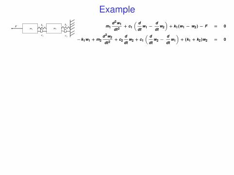
m1d2w1
dt2+ c1
„ d
dtw1 −
d
dtw2
«+ k1(w1 − w2)− F = 0
−k1w1 + m2d2w2
dt2+ c2
d
dtw2 + c1
„ d
dtw2 −
d
dtw1
«+ (k1 + k2)w2 = 0
Example
!
m1
!
m2
!
k1
!
k2
!
F
!
c1
!
c2
m1d2w1
dt2+ c1
„ d
dtw1 −
d
dtw2
«+ k1(w1 − w2)− F = 0
−k1w1 + m2d2w2
dt2+ c2
d
dtw2 + c1
„ d
dtw2 −
d
dtw1
«+ (k1 + k2)w2 = 0
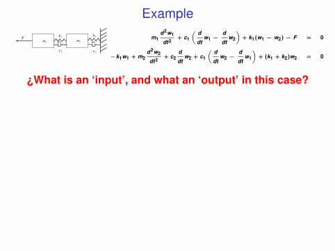
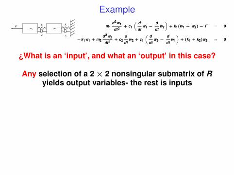
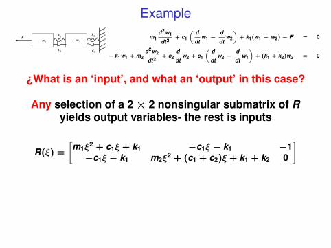
¿What is an ‘input’, and what an ‘output’ in this case?
Example
!
m1
!
m2
!
k1
!
k2
!
F
!
c1
!
c2
m1d2w1
dt2+ c1
„ d
dtw1 −
d
dtw2
«+ k1(w1 − w2)− F = 0
−k1w1 + m2d2w2
dt2+ c2
d
dtw2 + c1
„ d
dtw2 −
d
dtw1
«+ (k1 + k2)w2 = 0
¿What is an ‘input’, and what an ‘output’ in this case?
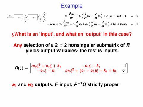
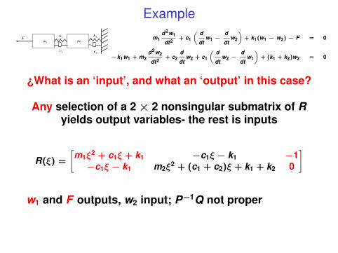
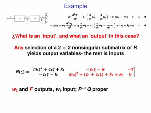
Any selection of a 2× 2 nonsingular submatrix of Ryields output variables- the rest is inputs
Example
!
m1
!
m2
!
k1
!
k2
!
F
!
c1
!
c2
m1d2w1
dt2+ c1
„ d
dtw1 −
d
dtw2
«+ k1(w1 − w2)− F = 0
−k1w1 + m2d2w2
dt2+ c2
d
dtw2 + c1
„ d
dtw2 −
d
dtw1
«+ (k1 + k2)w2 = 0
¿What is an ‘input’, and what an ‘output’ in this case?
Any selection of a 2× 2 nonsingular submatrix of Ryields output variables- the rest is inputs
R(ξ) =
[m1ξ
2 + c1ξ + k1 −c1ξ − k1 −1−c1ξ − k1 m2ξ
2 + (c1 + c2)ξ + k1 + k2 0
]
w1 and w2 outputs, F input; P−1Q strictly proper
Example
!
m1
!
m2
!
k1
!
k2
!
F
!
c1
!
c2
m1d2w1
dt2+ c1
„ d
dtw1 −
d
dtw2
«+ k1(w1 − w2)− F = 0
−k1w1 + m2d2w2
dt2+ c2
d
dtw2 + c1
„ d
dtw2 −
d
dtw1
«+ (k1 + k2)w2 = 0
¿What is an ‘input’, and what an ‘output’ in this case?
Any selection of a 2× 2 nonsingular submatrix of Ryields output variables- the rest is inputs
R(ξ) =
[m1ξ
2 + c1ξ + k1 −c1ξ − k1 −1−c1ξ − k1 m2ξ
2 + (c1 + c2)ξ + k1 + k2 0
]
w1 and F outputs, w2 input; P−1Q not proper
Example
!
m1
!
m2
!
k1
!
k2
!
F
!
c1
!
c2
m1d2w1
dt2+ c1
„ d
dtw1 −
d
dtw2
«+ k1(w1 − w2)− F = 0
−k1w1 + m2d2w2
dt2+ c2
d
dtw2 + c1
„ d
dtw2 −
d
dtw1
«+ (k1 + k2)w2 = 0
¿What is an ‘input’, and what an ‘output’ in this case?
Any selection of a 2× 2 nonsingular submatrix of Ryields output variables- the rest is inputs
R(ξ) =
[m1ξ
2 + c1ξ + k1 −c1ξ − k1 −1−c1ξ − k1 m2ξ
2 + (c1 + c2)ξ + k1 + k2 0
]
w2 and F outputs, w1 input; P−1Q proper
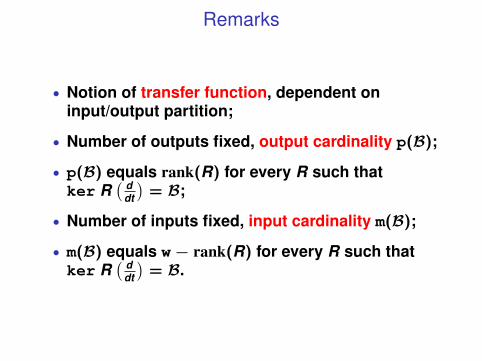
Remarks
• Notion of transfer function, dependent oninput/output partition;
• Number of outputs fixed, output cardinality p(B);
• p(B) equals rank(R) for every R such thatker R
( ddt
)= B;
• Number of inputs fixed, input cardinality m(B);
• m(B) equals w− rank(R) for every R such thatker R
( ddt
)= B.
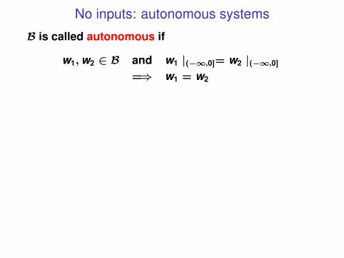
No inputs: autonomous systems
B is called autonomous if
w1,w2 ∈ B and w1 |(−∞,0]= w2 |(−∞,0]
=⇒ w1 = w2
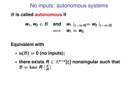
No inputs: autonomous systems
B is called autonomous if
w1,w2 ∈ B and w1 |(−∞,0]= w2 |(−∞,0]
=⇒ w1 = w2
Equivalent with
• m(B) = 0 (no inputs);
• there exists R ∈ Rw×w[ξ] nonsingular such thatB = ker R
( ddt
)
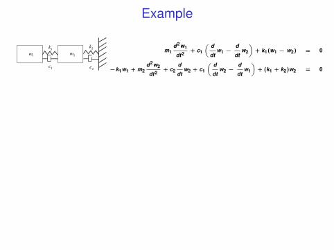
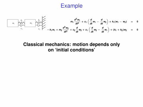
Example
!
m1
!
m2
!
k1
!
k2
!
c1
!
c2
m1d2w1
dt2+ c1
„ d
dtw1 −
d
dtw2
«+ k1(w1 − w2) = 0
−k1w1 + m2d2w2
dt2+ c2
d
dtw2 + c1
„ d
dtw2 −
d
dtw1
«+ (k1 + k2)w2 = 0
Example
!
m1
!
m2
!
k1
!
k2
!
c1
!
c2
m1d2w1
dt2+ c1
„ d
dtw1 −
d
dtw2
«+ k1(w1 − w2) = 0
−k1w1 + m2d2w2
dt2+ c2
d
dtw2 + c1
„ d
dtw2 −
d
dtw1
«+ (k1 + k2)w2 = 0
Classical mechanics: motion depends onlyon ‘initial conditions’
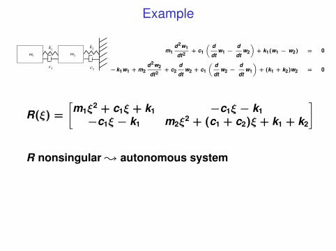
Example
!
m1
!
m2
!
k1
!
k2
!
c1
!
c2
m1d2w1
dt2+ c1
„ d
dtw1 −
d
dtw2
«+ k1(w1 − w2) = 0
−k1w1 + m2d2w2
dt2+ c2
d
dtw2 + c1
„ d
dtw2 −
d
dtw1
«+ (k1 + k2)w2 = 0
R(ξ) =
[m1ξ
2 + c1ξ + k1 −c1ξ − k1−c1ξ − k1 m2ξ
2 + (c1 + c2)ξ + k1 + k2
]
R nonsingular ; autonomous system
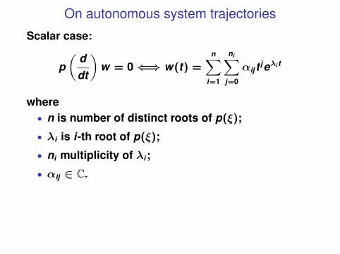
On autonomous system trajectories
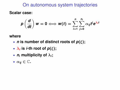
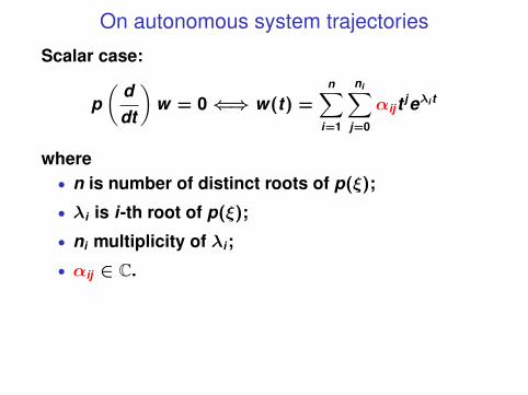
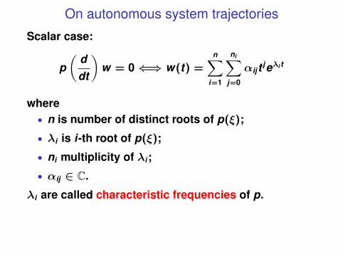
Scalar case:
p(
ddt
)w = 0⇐⇒ w(t) =
n∑i=1
ni∑j=0
αijt jeλi t
where• n is number of distinct roots of p(ξ);
• λi is i-th root of p(ξ);
• ni multiplicity of λi;
• αij ∈ C.
On autonomous system trajectories
Scalar case:
p(
ddt
)w = 0⇐⇒ w(t) =
n∑i=1
ni∑j=0
αijt jeλi t
where• n is number of distinct roots of p(ξ);
• λi is i-th root of p(ξ);
• ni multiplicity of λi;
• αij ∈ C.
On autonomous system trajectories
Scalar case:
p(
ddt
)w = 0⇐⇒ w(t) =
n∑i=1
ni∑j=0
αijt jeλi t
where• n is number of distinct roots of p(ξ);
• λi is i-th root of p(ξ);
• ni multiplicity of λi;
• αij ∈ C.

On autonomous system trajectories
Scalar case:
p(
ddt
)w = 0⇐⇒ w(t) =
n∑i=1
ni∑j=0
αijt jeλi t
where• n is number of distinct roots of p(ξ);
• λi is i-th root of p(ξ);
• ni multiplicity of λi;
• αij ∈ C.
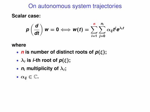
On autonomous system trajectories
Scalar case:
p(
ddt
)w = 0⇐⇒ w(t) =
n∑i=1
ni∑j=0
αijt jeλi t
where• n is number of distinct roots of p(ξ);
• λi is i-th root of p(ξ);
• ni multiplicity of λi;
• αij ∈ C.
On autonomous system trajectories
Scalar case:
p(
ddt
)w = 0⇐⇒ w(t) =
n∑i=1
ni∑j=0
αijt jeλi t
where• n is number of distinct roots of p(ξ);
• λi is i-th root of p(ξ);
• ni multiplicity of λi;
• αij ∈ C.
λi are called characteristic frequencies of p.
On autonomous system trajectories
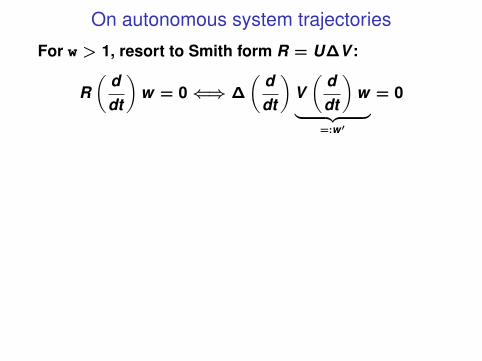
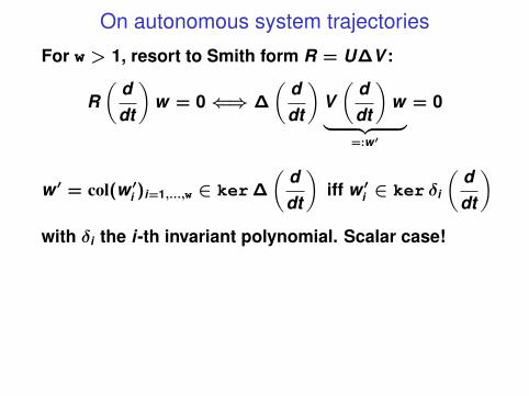
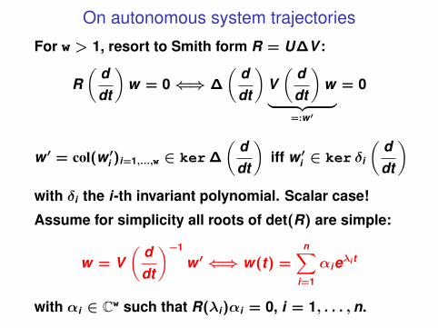
For w > 1, resort to Smith form R = U∆V :
R(
ddt
)w = 0⇐⇒ ∆
(ddt
)V(
ddt
)w︸ ︷︷ ︸
=:w ′
= 0
On autonomous system trajectories
For w > 1, resort to Smith form R = U∆V :
R(
ddt
)w = 0⇐⇒ ∆
(ddt
)V(
ddt
)w︸ ︷︷ ︸
=:w ′
= 0
w ′ = col(w ′i )i=1,...,w ∈ ker∆
(ddt
)iff w ′i ∈ ker δi
(ddt
)with δi the i-th invariant polynomial. Scalar case!
On autonomous system trajectories
For w > 1, resort to Smith form R = U∆V :
R(
ddt
)w = 0⇐⇒ ∆
(ddt
)V(
ddt
)w︸ ︷︷ ︸
=:w ′
= 0
w ′ = col(w ′i )i=1,...,w ∈ ker∆
(ddt
)iff w ′i ∈ ker δi
(ddt
)with δi the i-th invariant polynomial. Scalar case!
Assume for simplicity all roots of det(R) are simple:
w = V(
ddt
)−1
w ′ ⇐⇒ w(t) =n∑
i=1
αieλi t
with αi ∈ Cw such that R(λi)αi = 0, i = 1, . . . , n.
Remarks
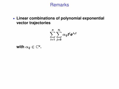
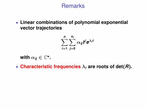
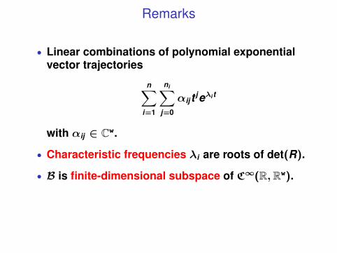
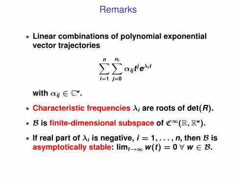
• Linear combinations of polynomial exponentialvector trajectories
n∑i=1
ni∑j=0
αijt jeλi t
with αij ∈ Cw.
• Characteristic frequencies λi are roots of det(R).
• B is finite-dimensional subspace of C∞(R,Rw).
• If real part of λi is negative, i = 1, . . . , n, then B isasymptotically stable: limt→∞w(t) = 0 ∀ w ∈ B.
Remarks
• Linear combinations of polynomial exponentialvector trajectories
n∑i=1
ni∑j=0
αijt jeλi t
with αij ∈ Cw.
• Characteristic frequencies λi are roots of det(R).
• B is finite-dimensional subspace of C∞(R,Rw).
• If real part of λi is negative, i = 1, . . . , n, then B isasymptotically stable: limt→∞w(t) = 0 ∀ w ∈ B.
Outline
Kernel and image representations
The Smith form
Surjectivity/injectivity of polynomial differential operators
Inputs and outputs
Controllability
Observability
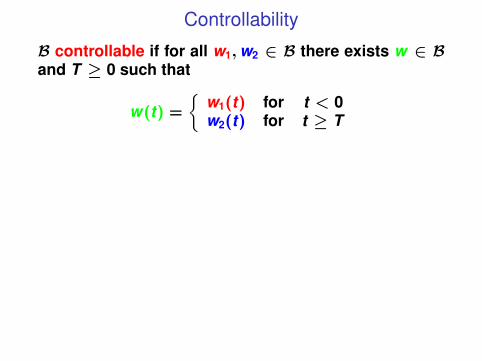
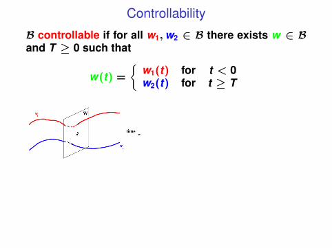
Controllability
B controllable if for all w1,w2 ∈ B there exists w ∈ Band T ≥ 0 such that
w(t) =
{w1(t) for t < 0w2(t) for t ≥ T
Controllability
B controllable if for all w1,w2 ∈ B there exists w ∈ Band T ≥ 0 such that
w(t) =
{w1(t) for t < 0w2(t) for t ≥ T
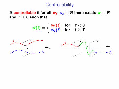
Controllability
B controllable if for all w1,w2 ∈ B there exists w ∈ Band T ≥ 0 such that
w(t) =
{w1(t) for t < 0w2(t) for t ≥ T
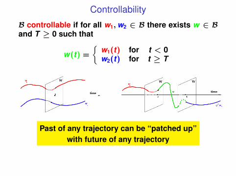
Controllability
B controllable if for all w1,w2 ∈ B there exists w ∈ Band T ≥ 0 such that
w(t) =
{w1(t) for t < 0w2(t) for t ≥ T
Past of any trajectory can be “patched up”with future of any trajectory
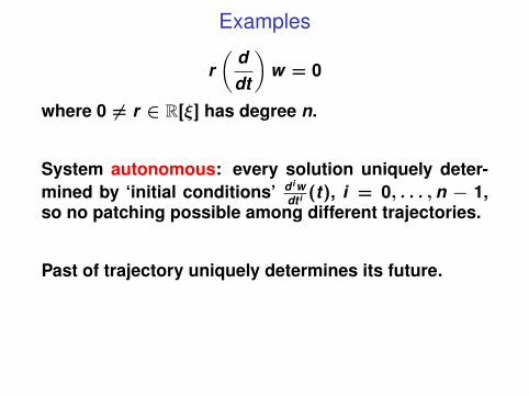
Examples
r(
ddt
)w = 0
where 0 6= r ∈ R[ξ] has degree n.
System autonomous: every solution uniquely deter-mined by ‘initial conditions’ d i w
dt i (t), i = 0, . . . , n − 1,so no patching possible among different trajectories.
Past of trajectory uniquely determines its future.
Bs controllable iff Bx controllable =⇒B controllable.
Examples
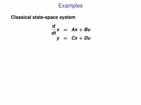
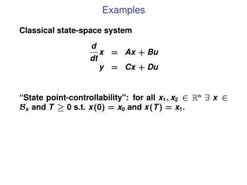
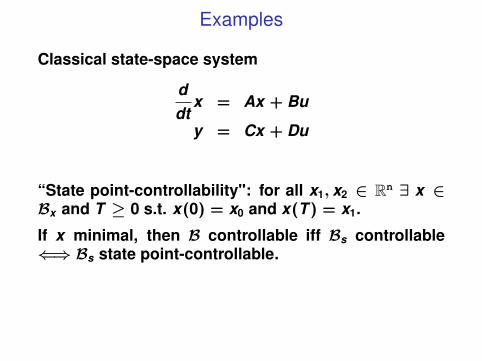
Classical state-space system
ddt
x = Ax + Bu
y = Cx + Du
Bs controllable iff Bx controllable =⇒B controllable.
Examples
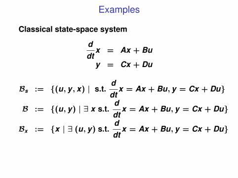
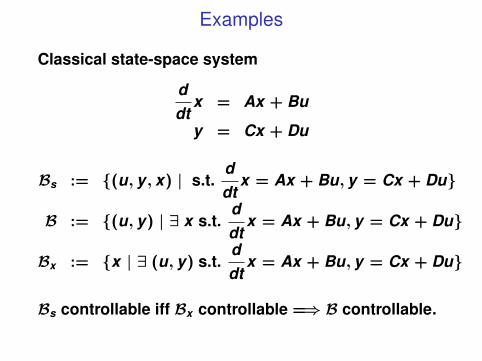
Classical state-space system
ddt
x = Ax + Bu
y = Cx + Du
Bs := {(u, y , x) | s.t.ddt
x = Ax + Bu, y = Cx + Du}
B := {(u, y) | ∃ x s.t.ddt
x = Ax + Bu, y = Cx + Du}
Bx := {x | ∃ (u, y) s.t.ddt
x = Ax + Bu, y = Cx + Du}
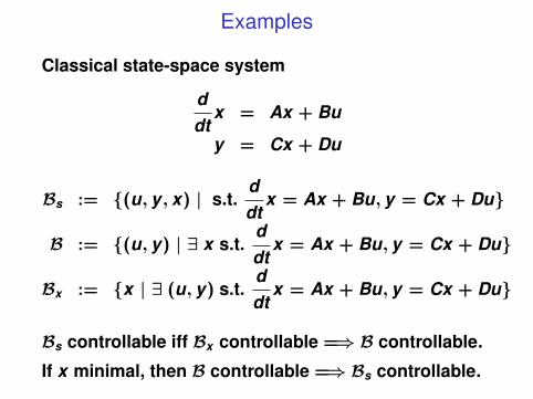
Bs controllable iff Bx controllable =⇒B controllable.
Examples
Classical state-space system
ddt
x = Ax + Bu
y = Cx + Du
Bs := {(u, y , x) | s.t.ddt
x = Ax + Bu, y = Cx + Du}
B := {(u, y) | ∃ x s.t.ddt
x = Ax + Bu, y = Cx + Du}
Bx := {x | ∃ (u, y) s.t.ddt
x = Ax + Bu, y = Cx + Du}
Bs controllable iff Bx controllable =⇒B controllable.
Examples
Classical state-space system
ddt
x = Ax + Bu
y = Cx + Du
Bs := {(u, y , x) | s.t.ddt
x = Ax + Bu, y = Cx + Du}
B := {(u, y) | ∃ x s.t.ddt
x = Ax + Bu, y = Cx + Du}
Bx := {x | ∃ (u, y) s.t.ddt
x = Ax + Bu, y = Cx + Du}
Bs controllable iff Bx controllable =⇒B controllable.
If x minimal, then B controllable =⇒Bs controllable.
Examples
Classical state-space system
ddt
x = Ax + Bu
y = Cx + Du
Bs controllable iff Bx controllable =⇒B controllable.
“State point-controllability": for all x1, x2 ∈ Rn ∃ x ∈Bx and T ≥ 0 s.t. x(0) = x0 and x(T ) = x1.
Examples
Classical state-space system
ddt
x = Ax + Bu
y = Cx + Du
Bs controllable iff Bx controllable =⇒B controllable.
“State point-controllability": for all x1, x2 ∈ Rn ∃ x ∈Bx and T ≥ 0 s.t. x(0) = x0 and x(T ) = x1.
If x minimal, then B controllable iff Bs controllable⇐⇒Bs state point-controllable.

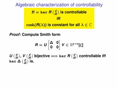
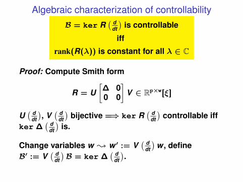
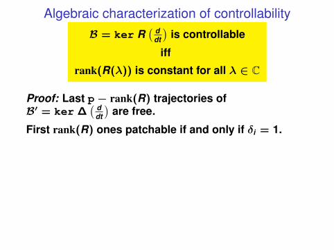
Algebraic characterization of controllabilityB = ker R
( ddt
)is controllable
iff
rank(R(λ)) is constant for all λ ∈ C
Algebraic characterization of controllabilityB = ker R
( ddt
)is controllable
iff
rank(R(λ)) is constant for all λ ∈ C
Proof: Compute Smith form
R = U[
∆ 00 0
]V ∈ Rp×w[ξ]
U( d
dt
), V( d
dt
)bijective =⇒ ker R
( ddt
)controllable iff
ker ∆( d
dt
)is.
Algebraic characterization of controllabilityB = ker R
( ddt
)is controllable
iff
rank(R(λ)) is constant for all λ ∈ C
Proof: Compute Smith form
R = U[
∆ 00 0
]V ∈ Rp×w[ξ]
U( d
dt
), V( d
dt
)bijective =⇒ ker R
( ddt
)controllable iff
ker ∆( d
dt
)is.
Change variables w ; w ′ := V( d
dt
)w , define
B′ := V( d
dt
)B = ker ∆
( ddt
).
Algebraic characterization of controllabilityB = ker R
( ddt
)is controllable
iff
rank(R(λ)) is constant for all λ ∈ C
Proof: Last p− rank(R) trajectories ofB′ = ker ∆
( ddt
)are free.
First rank(R) ones patchable if and only if δi = 1.
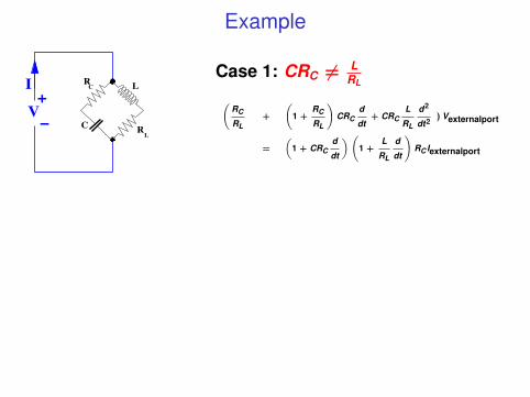
Example
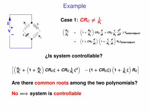
RLC circuit
Model the port behavior of
RL
C
C
LRI
V!
+
by tearing, zooming, and linking.
– p. 73/88
Case 1: CRC 6= LRL
RC
RL+
1 +
RC
RL
!CRC
d
dt+ CRC
L
RL
d2
dt2) Vexternalport
=
„1 + CRC
d
dt
« 1 +
L
RL
d
dt
!RC Iexternalport
Example
RLC circuit
Model the port behavior of
RL
C
C
LRI
V!
+
by tearing, zooming, and linking.
– p. 73/88
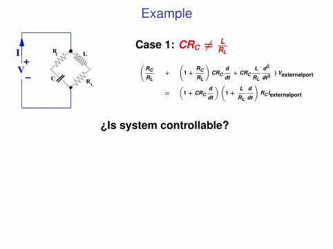
Case 1: CRC 6= LRL
RC
RL+
1 +
RC
RL
!CRC
d
dt+ CRC
L
RL
d2
dt2) Vexternalport
=
„1 + CRC
d
dt
« 1 +
L
RL
d
dt
!RC Iexternalport
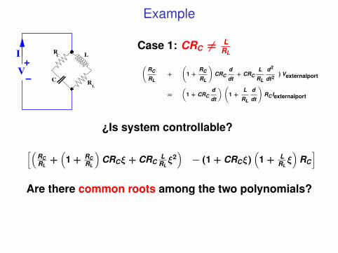
¿Is system controllable?
Example
RLC circuit
Model the port behavior of
RL
C
C
LRI
V!
+
by tearing, zooming, and linking.
– p. 73/88
Case 1: CRC 6= LRL
RC
RL+
1 +
RC
RL
!CRC
d
dt+ CRC
L
RL
d2
dt2) Vexternalport
=
„1 + CRC
d
dt
« 1 +
L
RL
d
dt
!RC Iexternalport
¿Is system controllable?
[(RCRL
+(
1 + RCRL
)CRCξ + CRC
LRLξ2)− (1 + CRCξ)
(1 + L
RLξ)
RC
]Are there common roots among the two polynomials?
No =⇒ system is controllable
Example
RLC circuit
Model the port behavior of
RL
C
C
LRI
V!
+
by tearing, zooming, and linking.
– p. 73/88
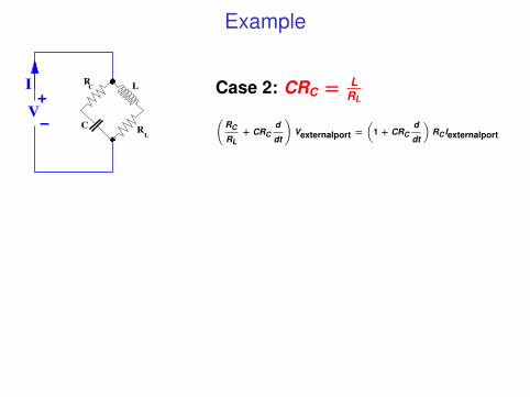
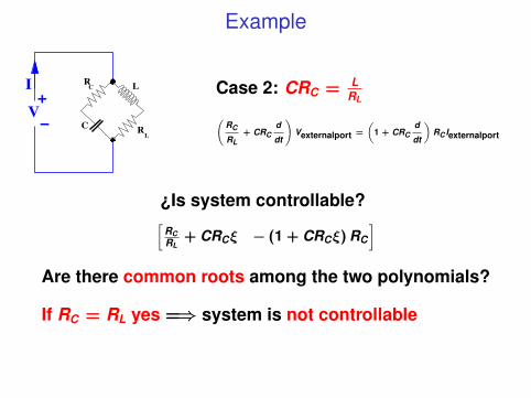
Case 2: CRC = LRL
RC
RL+ CRC
d
dt
!Vexternalport =
„1 + CRC
d
dt
«RC Iexternalport
Example
RLC circuit
Model the port behavior of
RL
C
C
LRI
V!
+
by tearing, zooming, and linking.
– p. 73/88
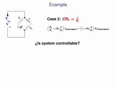
Case 2: CRC = LRL
RC
RL+ CRC
d
dt
!Vexternalport =
„1 + CRC
d
dt
«RC Iexternalport
¿Is system controllable?
Example
RLC circuit
Model the port behavior of
RL
C
C
LRI
V!
+
by tearing, zooming, and linking.
– p. 73/88
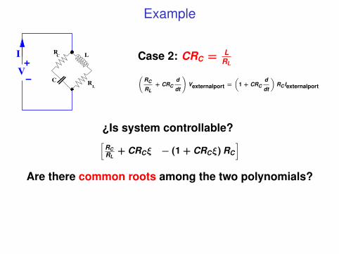
Case 2: CRC = LRL
RC
RL+ CRC
d
dt
!Vexternalport =
„1 + CRC
d
dt
«RC Iexternalport
¿Is system controllable?[RCRL
+ CRCξ − (1 + CRCξ) RC
]Are there common roots among the two polynomials?
Example
RLC circuit
Model the port behavior of
RL
C
C
LRI
V!
+
by tearing, zooming, and linking.
– p. 73/88
Case 2: CRC = LRL
RC
RL+ CRC
d
dt
!Vexternalport =
„1 + CRC
d
dt
«RC Iexternalport
¿Is system controllable?[RCRL
+ CRCξ − (1 + CRCξ) RC
]Are there common roots among the two polynomials?
If RC = RL yes =⇒ system is not controllable
Remarks
• B = ker R( d
dt
), with R ∈ Rw×w[ξ] nonsingular, is
controllable⇐⇒ R is unimodular⇐⇒B = {0}
• Rank constancy test generalization of ‘Hautustest’ for state-space systems.
• Trajectory-, not representation-based definition asin state-space framework.
Remarks
• B = ker R( d
dt
), with R ∈ Rw×w[ξ] nonsingular, is
controllable⇐⇒ R is unimodular⇐⇒B = {0}
• Rank constancy test generalization of ‘Hautustest’ for state-space systems.
• Trajectory-, not representation-based definition asin state-space framework.
Remarks
• B = ker R( d
dt
), with R ∈ Rw×w[ξ] nonsingular, is
controllable⇐⇒ R is unimodular⇐⇒B = {0}
• Rank constancy test generalization of ‘Hautustest’ for state-space systems.
• Trajectory-, not representation-based definition asin state-space framework.
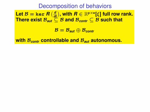
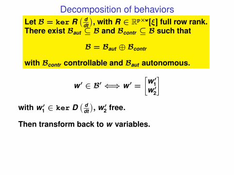
Decomposition of behaviorsLet B = ker R
( ddt
), with R ∈ Rp×w[ξ] full row rank.
There exist Baut ⊆ B and Bcontr ⊆ B such that
B = Baut ⊕ Bcontr
with Bcontr controllable and Baut autonomous.
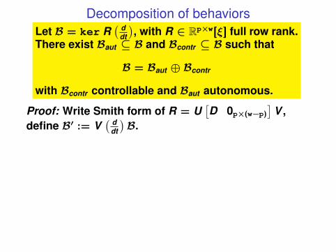
Decomposition of behaviorsLet B = ker R
( ddt
), with R ∈ Rp×w[ξ] full row rank.
There exist Baut ⊆ B and Bcontr ⊆ B such that
B = Baut ⊕ Bcontr
with Bcontr controllable and Baut autonomous.
Proof: Write Smith form of R = U[D 0p×(w−p)
]V ,
define B′ := V( d
dt
)B.
Decomposition of behaviorsLet B = ker R
( ddt
), with R ∈ Rp×w[ξ] full row rank.
There exist Baut ⊆ B and Bcontr ⊆ B such that
B = Baut ⊕ Bcontr
with Bcontr controllable and Baut autonomous.
Proof: Write Smith form of R = U[D 0p×(w−p)
]V ,
define B′ := V( d
dt
)B.
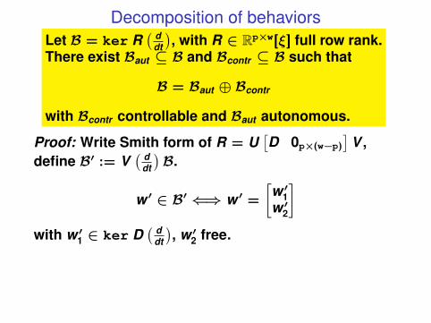
w ′ ∈ B′ ⇐⇒ w ′ =
[w ′1w ′2
]with w ′1 ∈ ker D
( ddt
), w ′2 free.

Decomposition of behaviorsLet B = ker R
( ddt
), with R ∈ Rp×w[ξ] full row rank.
There exist Baut ⊆ B and Bcontr ⊆ B such that
B = Baut ⊕ Bcontr
with Bcontr controllable and Baut autonomous.
w ′ ∈ B′ ⇐⇒ w ′ =
[w ′1w ′2
]with w ′1 ∈ ker D
( ddt
), w ′2 free.
If D = Ip =⇒ take B′contr
= B′, B′aut
= {0}.
Decomposition of behaviorsLet B = ker R
( ddt
), with R ∈ Rp×w[ξ] full row rank.
There exist Baut ⊆ B and Bcontr ⊆ B such that
B = Baut ⊕ Bcontr
with Bcontr controllable and Baut autonomous.
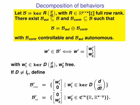
w ′ ∈ B′ ⇐⇒ w ′ =
[w ′1w ′2
]with w ′1 ∈ ker D
( ddt
), w ′2 free.
If D 6= Ip, define
B′contr
= {[w ′10
]| w ′1 ∈ ker D
(ddt
)}
B′aut
= {[
0w ′2
]| w ′2 ∈ C∞(R,Rw−p)}.
Decomposition of behaviorsLet B = ker R
( ddt
), with R ∈ Rp×w[ξ] full row rank.
There exist Baut ⊆ B and Bcontr ⊆ B such that
B = Baut ⊕ Bcontr
with Bcontr controllable and Baut autonomous.
w ′ ∈ B′ ⇐⇒ w ′ =
[w ′1w ′2
]with w ′1 ∈ ker D
( ddt
), w ′2 free.
Then transform back to w variables.
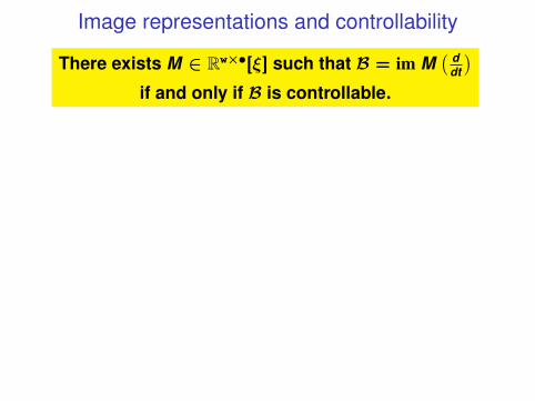
Image representations and controllability
There exists M ∈ Rwו[ξ] such that B = im M( d
dt
)if and only if B is controllable.
Note also that M can be chosen with m(B) columns.
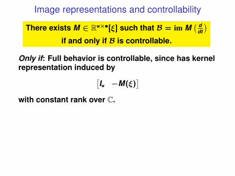
Image representations and controllability
There exists M ∈ Rwו[ξ] such that B = im M( d
dt
)if and only if B is controllable.
Only if: Full behavior is controllable, since has kernelrepresentation induced by[
Iw −M(ξ)]
with constant rank over C.
Note also that M can be chosen with m(B) columns.
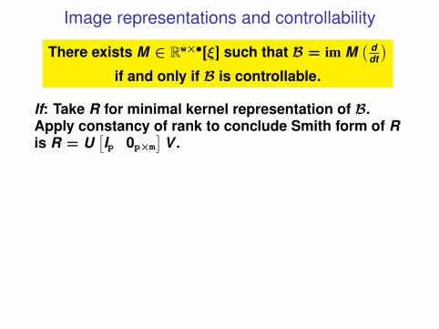
Image representations and controllability
There exists M ∈ Rwו[ξ] such that B = im M( d
dt
)if and only if B is controllable.
If: Take R for minimal kernel representation of B.Apply constancy of rank to conclude Smith form of Ris R = U
[Ip 0p×m
]V .
Note also that M can be chosen with m(B) columns.
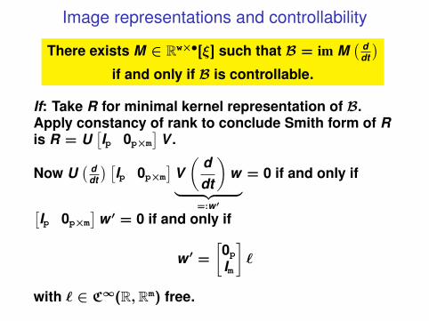
Image representations and controllability
There exists M ∈ Rwו[ξ] such that B = im M( d
dt
)if and only if B is controllable.
If: Take R for minimal kernel representation of B.Apply constancy of rank to conclude Smith form of Ris R = U
[Ip 0p×m
]V .
Now U( d
dt
) [Ip 0p×m
]V(
ddt
)w︸ ︷︷ ︸
=:w ′
= 0 if and only if
[Ip 0p×m
]w ′ = 0 if and only if
w ′ =
[0pIm
]`
with ` ∈ C∞(R,Rm) free.
Note also that M can be chosen with m(B) columns.
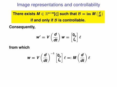
Image representations and controllability
There exists M ∈ Rwו[ξ] such that B = im M( d
dt
)if and only if B is controllable.
Consequently,
w ′ = V(
ddt
)w =
[0pIm
]`
from which
w = V(
ddt
)−1 [0pIm
]` =: M
(ddt
)`
Note also that M can be chosen with m(B) columns.
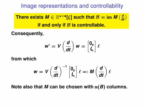
Image representations and controllability
There exists M ∈ Rwו[ξ] such that B = im M( d
dt
)if and only if B is controllable.
Consequently,
w ′ = V(
ddt
)w =
[0pIm
]`
from which
w = V(
ddt
)−1 [0pIm
]` =: M
(ddt
)`
Note also that M can be chosen with m(B) columns.
Outline
Kernel and image representations
The Smith form
Surjectivity/injectivity of polynomial differential operators
Inputs and outputs
Controllability
Observability
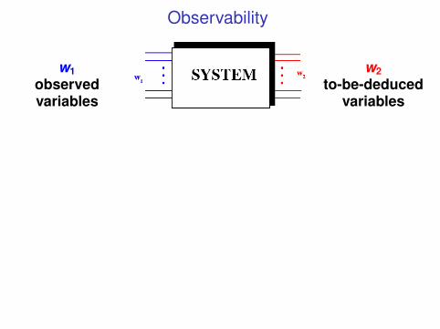
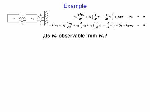
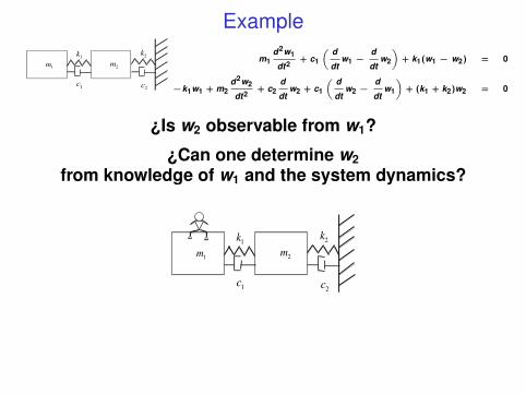
Observability
w1observedvariables
w2to-be-deduced
variables
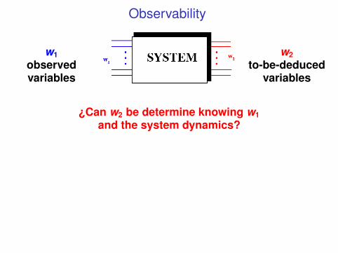
Observability
w1observedvariables
w2to-be-deduced
variables
¿Can w2 be determine knowing w1and the system dynamics?
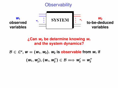
Observability
w1observedvariables
w2to-be-deduced
variables
¿Can w2 be determine knowing w1and the system dynamics?
B ∈ Lw, w = (w1,w2). w2 is observable from w1 if
(w1,w ′2), (w1,w ′′2 ) ∈ B =⇒ w ′2 = w ′′2
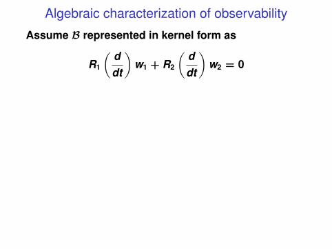
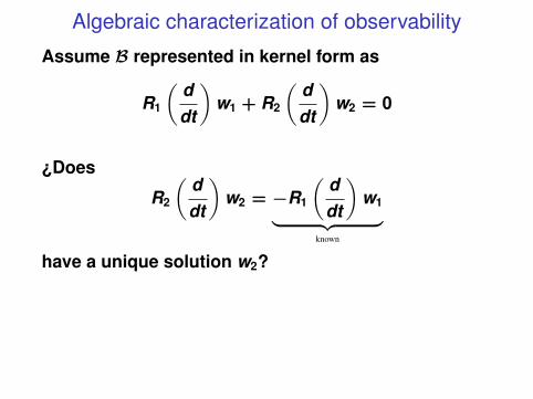
Algebraic characterization of observability
Assume B represented in kernel form as
R1
(ddt
)w1 + R2
(ddt
)w2 = 0
Algebraic characterization of observability
Assume B represented in kernel form as
R1
(ddt
)w1 + R2
(ddt
)w2 = 0
¿Does
R2
(ddt
)w2 = −R1
(ddt
)w1︸ ︷︷ ︸
known
have a unique solution w2?
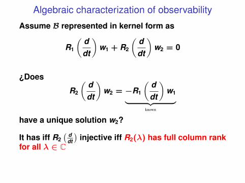
Algebraic characterization of observability
Assume B represented in kernel form as
R1
(ddt
)w1 + R2
(ddt
)w2 = 0
¿Does
R2
(ddt
)w2 = −R1
(ddt
)w1︸ ︷︷ ︸
known
have a unique solution w2?
It has iff R2( d
dt
)injective iff R2(λ) has full column rank
for all λ ∈ C
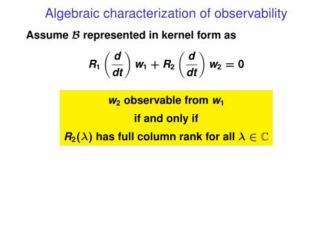
Algebraic characterization of observability
Assume B represented in kernel form as
R1
(ddt
)w1 + R2
(ddt
)w2 = 0
w2 observable from w1
if and only if
R2(λ) has full column rank for all λ ∈ C
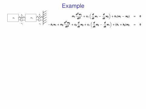
Example
!
m1
!
m2
!
k1
!
k2
!
c1
!
c2
m1d2w1
dt2+ c1
„ d
dtw1 −
d
dtw2
«+ k1(w1 − w2) = 0
−k1w1 + m2d2w2
dt2+ c2
d
dtw2 + c1
„ d
dtw2 −
d
dtw1
«+ (k1 + k2)w2 = 0
[c1λ + k1
−m2λ2 − (c2 + c1)λ− (k1 + k2)
]has full column rank ∀ λ ∈ C (⇐⇒ observability) iff
−m2k 21 + c1c2k1 − k2c2
2 6= 0
Example
!
m1
!
m2
!
k1
!
k2
!
c1
!
c2
m1d2w1
dt2+ c1
„ d
dtw1 −
d
dtw2
«+ k1(w1 − w2) = 0
−k1w1 + m2d2w2
dt2+ c2
d
dtw2 + c1
„ d
dtw2 −
d
dtw1
«+ (k1 + k2)w2 = 0
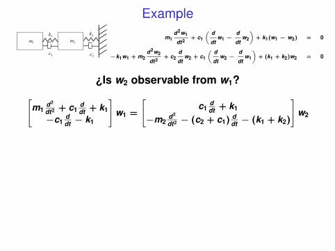
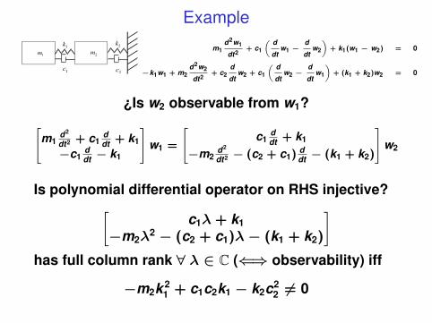
¿Is w2 observable from w1?
[c1λ + k1
−m2λ2 − (c2 + c1)λ− (k1 + k2)
]has full column rank ∀ λ ∈ C (⇐⇒ observability) iff
−m2k 21 + c1c2k1 − k2c2
2 6= 0
Example
!
m1
!
m2
!
k1
!
k2
!
c1
!
c2
m1d2w1
dt2+ c1
„ d
dtw1 −
d
dtw2
«+ k1(w1 − w2) = 0
−k1w1 + m2d2w2
dt2+ c2
d
dtw2 + c1
„ d
dtw2 −
d
dtw1
«+ (k1 + k2)w2 = 0
¿Is w2 observable from w1?
¿Can one determine w2from knowledge of w1 and the system dynamics?
!
m1
!
m2
!
k1
!
k2
!
c1
!
c2
[c1λ + k1
−m2λ2 − (c2 + c1)λ− (k1 + k2)
]has full column rank ∀ λ ∈ C (⇐⇒ observability) iff
−m2k 21 + c1c2k1 − k2c2
2 6= 0
Example
!
m1
!
m2
!
k1
!
k2
!
c1
!
c2
m1d2w1
dt2+ c1
„ d
dtw1 −
d
dtw2
«+ k1(w1 − w2) = 0
−k1w1 + m2d2w2
dt2+ c2
d
dtw2 + c1
„ d
dtw2 −
d
dtw1
«+ (k1 + k2)w2 = 0
¿Is w2 observable from w1?[m1
d2
dt2 + c1ddt + k1
−c1ddt − k1
]w1 =
[c1
ddt + k1
−m2d2
dt2 − (c2 + c1) ddt − (k1 + k2)
]w2
[c1λ + k1
−m2λ2 − (c2 + c1)λ− (k1 + k2)
]has full column rank ∀ λ ∈ C (⇐⇒ observability) iff
−m2k21 + c1c2k1 − k2c2
2 6= 0
Example
!
m1
!
m2
!
k1
!
k2
!
c1
!
c2
m1d2w1
dt2+ c1
„ d
dtw1 −
d
dtw2
«+ k1(w1 − w2) = 0
−k1w1 + m2d2w2
dt2+ c2
d
dtw2 + c1
„ d
dtw2 −
d
dtw1
«+ (k1 + k2)w2 = 0
¿Is w2 observable from w1?[m1
d2
dt2 + c1ddt + k1
−c1ddt − k1
]w1 =
[c1
ddt + k1
−m2d2
dt2 − (c2 + c1) ddt − (k1 + k2)
]w2
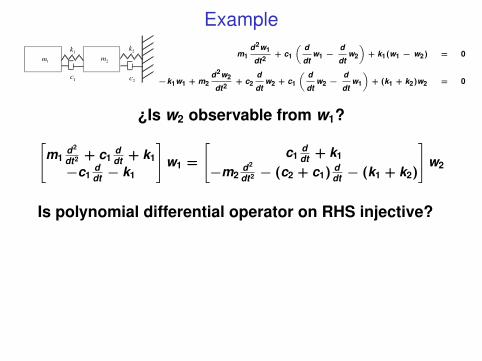
Is polynomial differential operator on RHS injective?
[c1λ + k1
−m2λ2 − (c2 + c1)λ− (k1 + k2)
]has full column rank ∀ λ ∈ C (⇐⇒ observability) iff
−m2k 21 + c1c2k1 − k2c2
2 6= 0
Example
!
m1
!
m2
!
k1
!
k2
!
c1
!
c2
m1d2w1
dt2+ c1
„ d
dtw1 −
d
dtw2
«+ k1(w1 − w2) = 0
−k1w1 + m2d2w2
dt2+ c2
d
dtw2 + c1
„ d
dtw2 −
d
dtw1
«+ (k1 + k2)w2 = 0
¿Is w2 observable from w1?[m1
d2
dt2 + c1ddt + k1
−c1ddt − k1
]w1 =
[c1
ddt + k1
−m2d2
dt2 − (c2 + c1) ddt − (k1 + k2)
]w2
Is polynomial differential operator on RHS injective?[c1λ + k1
−m2λ2 − (c2 + c1)λ− (k1 + k2)
]has full column rank ∀ λ ∈ C (⇐⇒ observability) iff
−m2k 21 + c1c2k1 − k2c2
2 6= 0

Remarks
• Rank constancy test generalization of ‘Hautustest’ for state-space systems.
• Trajectory-, not representation-based definitionas in state-space framework.
Remarks
• Rank constancy test generalization of ‘Hautustest’ for state-space systems.
• Trajectory-, not representation-based definitionas in state-space framework.

Summary
• Polynomial differential operators and theirproperties are key;
• Inputs: free variables;
• Autonomous systems;
• Controllability and observability;
• Algebraic characterizations;
• Image representations.
Summary
• Polynomial differential operators and theirproperties are key;
• Inputs: free variables;
• Autonomous systems;
• Controllability and observability;
• Algebraic characterizations;
• Image representations.
Summary
• Polynomial differential operators and theirproperties are key;
• Inputs: free variables;
• Autonomous systems;
• Controllability and observability;
• Algebraic characterizations;
• Image representations.
Summary
• Polynomial differential operators and theirproperties are key;
• Inputs: free variables;
• Autonomous systems;
• Controllability and observability;
• Algebraic characterizations;
• Image representations.
Summary
• Polynomial differential operators and theirproperties are key;
• Inputs: free variables;
• Autonomous systems;
• Controllability and observability;
• Algebraic characterizations;
• Image representations.
Summary
• Polynomial differential operators and theirproperties are key;
• Inputs: free variables;
• Autonomous systems;
• Controllability and observability;
• Algebraic characterizations;
• Image representations.