SLEPc: Scalable Library for Eigenvalue Problem Computations
69
Introduction Overview of SLEPc Basic Usage Advanced Features SLEPc: Scalable Library for Eigenvalue Problem Computations Jose E. Roman Joint work with A. Tomas and E. Romero Universidad Polit´ ecnica de Valencia, Spain 10th ACTS Workshop - August, 2009
Transcript of SLEPc: Scalable Library for Eigenvalue Problem Computations

IntroductionOverview of SLEPc
Basic UsageAdvanced Features
SLEPc: Scalable Library for Eigenvalue ProblemComputations
Jose E. Roman
Joint work with A. Tomas and E. Romero
Universidad Politecnica de Valencia, Spain
10th ACTS Workshop - August, 2009
IntroductionOverview of SLEPc
Basic UsageAdvanced Features
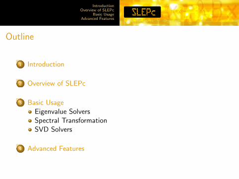
Outline
1 Introduction
2 Overview of SLEPc
3 Basic UsageEigenvalue SolversSpectral TransformationSVD Solvers
4 Advanced Features

IntroductionOverview of SLEPc
Basic UsageAdvanced Features
Introduction

IntroductionOverview of SLEPc
Basic UsageAdvanced Features
Eigenvalue Problems
Consider the following eigenvalue problems
Standard Eigenproblem
Ax = λx
Generalized Eigenproblem
Ax = λBx
where
I λ is a (complex) scalar: eigenvalue
I x is a (complex) vector: eigenvector
I Matrices A and B can be real or complex
I Matrices A and B can be symmetric (Hermitian) or not
I Typically, B is symmetric positive (semi-) definite

IntroductionOverview of SLEPc
Basic UsageAdvanced Features
Solution of the Eigenvalue Problem
There are n eigenvalues (counted with their multiplicities)
Partial eigensolution: nev solutions
λ0, λ1, . . . , λnev−1 ∈ Cx0, x1, . . . , xnev−1 ∈ Cn
nev = number ofeigenvalues /eigenvectors(eigenpairs)
Different requirements:
I Compute a few of the dominant eigenvalues (largestmagnitude)
I Compute a few λi’s with smallest or largest real parts
I Compute all λi’s in a certain region of the complex plane

IntroductionOverview of SLEPc
Basic UsageAdvanced Features
Spectral Transformation
A general technique that can be used in many methods
Ax = λx =⇒ Tx = θx
In the transformed problem
I The eigenvectors are not altered
I The eigenvalues are modified by a simple relation
I Convergence is usually improved (better separation)
Shift of Origin
TS = A + σI
Shift-and-invert
TSI = (A−σI)−1
Cayley
TC = (A−σI)−1(A+τI)
Drawback: T not computed explicitly, linear solves instead
IntroductionOverview of SLEPc
Basic UsageAdvanced Features
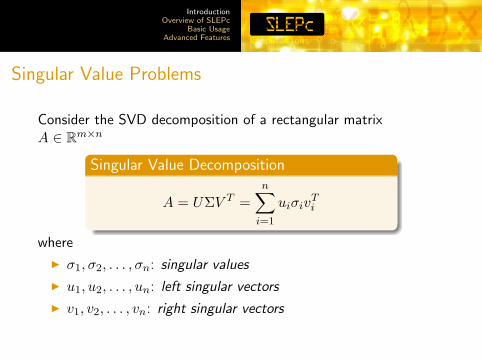
Singular Value Problems
Consider the SVD decomposition of a rectangular matrixA ∈ Rm×n
Singular Value Decomposition
A = UΣV T =n∑
i=1
uiσivTi
where
I σ1, σ2, . . . , σn: singular values
I u1, u2, . . . , un: left singular vectors
I v1, v2, . . . , vn: right singular vectors

IntroductionOverview of SLEPc
Basic UsageAdvanced Features
Solution of the Singular Value Problem
There are n singular values (counted with their multiplicities)
Partial solution: nsv solutions
σ0, σ1, . . . , σnsv−1 ∈ Ru0, u1, . . . , unsv−1 ∈ Rm
v0, v1, . . . , vnsv−1 ∈ Rn
nsv = number ofsingular values /vectors (singulartriplets)
I Compute a few smallest or largest σi’s
Alternatives:
I Solve eigenproblem AT A
I Solve eigenproblem H(A) =[
0m×m AAT 0n×n
]I Bidiagonalization

IntroductionOverview of SLEPc
Basic UsageAdvanced Features
Overview of SLEPc

IntroductionOverview of SLEPc
Basic UsageAdvanced Features
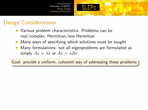
Design ConsiderationsI Various problem characteristics: Problems can be
real/complex, Hermitian/non-HermitianI Many ways of specifying which solutions must be soughtI Many formulations: not all eigenproblems are formulated as
simply Ax = λx or Ax = λBx
Goal: provide a uniform, coherent way of addressing these problems
I Internally, solvers can be quite complex (deflation, restart, ...)I Spectral transformations can be used irrespective of the solverI Repeated linear solves may be requiredI SVD can be solved via associated eigenproblem or
bidiagonalization
Goal: hide eigensolver complexity and separate spectral transform
IntroductionOverview of SLEPc
Basic UsageAdvanced Features
Design ConsiderationsI Various problem characteristics: Problems can be
real/complex, Hermitian/non-HermitianI Many ways of specifying which solutions must be soughtI Many formulations: not all eigenproblems are formulated as
simply Ax = λx or Ax = λBx
Goal: provide a uniform, coherent way of addressing these problems
I Internally, solvers can be quite complex (deflation, restart, ...)I Spectral transformations can be used irrespective of the solverI Repeated linear solves may be requiredI SVD can be solved via associated eigenproblem or
bidiagonalization
Goal: hide eigensolver complexity and separate spectral transform

IntroductionOverview of SLEPc
Basic UsageAdvanced Features
What Users Need
Provided by PETSc
I Abstraction of mathematical objects: vectors and matrices
I Efficient linear solvers (direct or iterative)
I Easy programming interface
I Run-time flexibility, full control over the solution process
I Parallel computing, mostly transparent to the user
Provided by SLEPc
I State-of-the-art eigensolvers
I Spectral transformations
I SVD solvers

IntroductionOverview of SLEPc
Basic UsageAdvanced Features
Summary
PETSc: Portable, Extensible Toolkit for Scientific Computation
Software for the scalable (parallel) solution of algebraic systemsarising from partial differential equation (PDE) simulations
I Developed at Argonne National Lab since 1991
I Usable from C, C++, Fortran77/90
I Focus on abstraction, portability, interoperability
I Extensive documentation and examples
I Freely available and supported through email
http://www.mcs.anl.gov/petsc
Current version: 3.0.0 (released Dec 2008)

IntroductionOverview of SLEPc
Basic UsageAdvanced Features
Summary
SLEPc: Scalable Library for Eigenvalue Problem Computations
A general library for solving large-scale sparse eigenproblems onparallel computers
I For standard and generalized eigenproblems
I For real and complex arithmetic
I For Hermitian or non-Hermitian problems
Also support for the partial SVD decomposition
http://www.grycap.upv.es/slepc
Current version: 3.0.0 (released Feb 2009)

IntroductionOverview of SLEPc
Basic UsageAdvanced Features
Structure of SLEPc (1)
SLEPc extends PETSc with three new objects: EPS, ST, SVD
EPS: Eigenvalue Problem Solver
I The user specifies an eigenproblem via this object
I Provides a collection of eigensolvers
I Allows the user to specify a number of parameters (e.g. whichportion of the spectrum)

IntroductionOverview of SLEPc
Basic UsageAdvanced Features
Structure of SLEPc (2)
ST: Spectral Transformation
I Used to transform the original problem into Tx = θx
I Always associated to an EPS object, not used directly
SVD: Singular Value Decomposition
I The user specifies the SVD problem via this object
I Transparently provides the associated eigenproblems or aspecialized solver

IntroductionOverview of SLEPc
Basic UsageAdvanced Features
PETSc/SLEPc Numerical ComponentsPETSc
Vectors
Index Sets
Indices Block Indices Stride Other
Matrices
CompressedSparse Row
Block CompressedSparse Row
BlockDiagonal Dense Other
Preconditioners
AdditiveSchwarz
BlockJacobi
Jacobi ILU ICC LU Other
Krylov Subspace Methods
GMRES CG CGS Bi-CGStab TFQMR Richardson Chebychev Other
Nonlinear Systems
LineSearch
TrustRegion Other
Time Steppers
EulerBackward
Euler
PseudoTime Step Other
SLEPc
SVD Solvers
CrossProduct
CyclicMatrix
LanczosThick Res.Lanczos
Eigensolvers
Krylov-Schur Arnoldi Lanczos Other
Spectral Transform
Shift Shift-and-invert Cayley Fold

IntroductionOverview of SLEPc
Basic UsageAdvanced Features
Basic Usage

IntroductionOverview of SLEPc
Basic UsageAdvanced Features
EPS: Basic Usage
Usual steps for solving an eigenvalue problem with SLEPc:
1. Create an EPS object
2. Define the eigenvalue problem
3. (Optionally) Specify options for the solution
4. Run the eigensolver
5. Retrieve the computed solution
6. Destroy the EPS object
All these operations are done via a generic interface, common toall the eigensolvers

IntroductionOverview of SLEPc
Basic UsageAdvanced Features
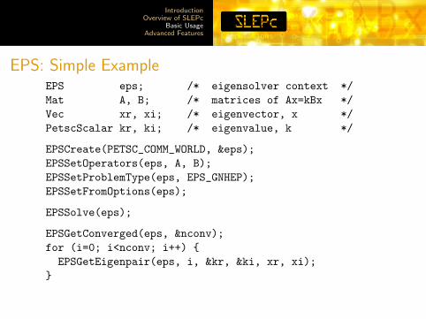
EPS: Simple ExampleEPS eps; /* eigensolver context */Mat A, B; /* matrices of Ax=kBx */Vec xr, xi; /* eigenvector, x */PetscScalar kr, ki; /* eigenvalue, k */
EPSCreate(PETSC_COMM_WORLD, &eps);EPSSetOperators(eps, A, B);EPSSetProblemType(eps, EPS_GNHEP);EPSSetFromOptions(eps);
EPSSolve(eps);
EPSGetConverged(eps, &nconv);for (i=0; i<nconv; i++) {EPSGetEigenpair(eps, i, &kr, &ki, xr, xi);
}
EPSDestroy(eps);

IntroductionOverview of SLEPc
Basic UsageAdvanced Features
EPS: Simple ExampleEPS eps; /* eigensolver context */Mat A, B; /* matrices of Ax=kBx */Vec xr, xi; /* eigenvector, x */PetscScalar kr, ki; /* eigenvalue, k */
EPSCreate(PETSC_COMM_WORLD, &eps);EPSSetOperators(eps, A, B);EPSSetProblemType(eps, EPS_GNHEP);EPSSetFromOptions(eps);
EPSSolve(eps);
EPSGetConverged(eps, &nconv);for (i=0; i<nconv; i++) {EPSGetEigenpair(eps, i, &kr, &ki, xr, xi);
}
EPSDestroy(eps);

IntroductionOverview of SLEPc
Basic UsageAdvanced Features
Details: Solving the Problem
EPSSolve(EPS eps)
Launches the eigensolver
Currently available eigensolvers:
I Power Iteration and RQI
I Subspace Iteration with Rayleigh-Ritz projection and locking
I Arnoldi method with explicit restart and deflationI Lanczos method with explicit restart and deflation
I Reorthogonalization: Local, Partial, Periodic, Selective, Full
I Krylov-Schur (default)
Also interfaces to external software: ARPACK, PRIMME, ...
IntroductionOverview of SLEPc
Basic UsageAdvanced Features
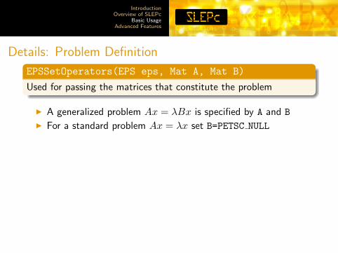
Details: Problem Definition
EPSSetOperators(EPS eps, Mat A, Mat B)
Used for passing the matrices that constitute the problem
I A generalized problem Ax = λBx is specified by A and BI For a standard problem Ax = λx set B=PETSC NULL
EPSSetProblemType(EPS eps,EPSProblemType type)
Used to indicate the problem type
Problem Type EPSProblemType Command line keyHermitian EPS HEP -eps hermitianGeneralized Hermitian EPS GHEP -eps gen hermitianNon-Hermitian EPS NHEP -eps non hermitianGeneralized Non-Herm. EPS GNHEP -eps gen non hermitian

IntroductionOverview of SLEPc
Basic UsageAdvanced Features
Details: Problem Definition
EPSSetOperators(EPS eps, Mat A, Mat B)
Used for passing the matrices that constitute the problem
I A generalized problem Ax = λBx is specified by A and BI For a standard problem Ax = λx set B=PETSC NULL
EPSSetProblemType(EPS eps,EPSProblemType type)
Used to indicate the problem type
Problem Type EPSProblemType Command line keyHermitian EPS HEP -eps hermitianGeneralized Hermitian EPS GHEP -eps gen hermitianNon-Hermitian EPS NHEP -eps non hermitianGeneralized Non-Herm. EPS GNHEP -eps gen non hermitian
IntroductionOverview of SLEPc
Basic UsageAdvanced Features
Details: Specification of Options
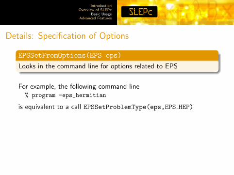
EPSSetFromOptions(EPS eps)
Looks in the command line for options related to EPS
For example, the following command line% program -eps_hermitian
is equivalent to a call EPSSetProblemType(eps,EPS HEP)
Other options have an associated function call% program -eps_nev 6 -eps_tol 1e-8
EPSView(EPS eps, PetscViewer viewer)
Prints information about the object (equivalent to -eps view)

IntroductionOverview of SLEPc
Basic UsageAdvanced Features
Details: Specification of Options
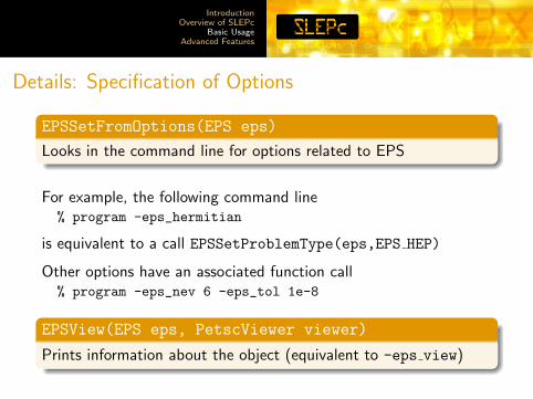
EPSSetFromOptions(EPS eps)
Looks in the command line for options related to EPS
For example, the following command line% program -eps_hermitian
is equivalent to a call EPSSetProblemType(eps,EPS HEP)
Other options have an associated function call% program -eps_nev 6 -eps_tol 1e-8
EPSView(EPS eps, PetscViewer viewer)
Prints information about the object (equivalent to -eps view)
IntroductionOverview of SLEPc
Basic UsageAdvanced Features
Details: Specification of Options
EPSSetFromOptions(EPS eps)
Looks in the command line for options related to EPS
For example, the following command line% program -eps_hermitian
is equivalent to a call EPSSetProblemType(eps,EPS HEP)
Other options have an associated function call% program -eps_nev 6 -eps_tol 1e-8
EPSView(EPS eps, PetscViewer viewer)
Prints information about the object (equivalent to -eps view)
IntroductionOverview of SLEPc
Basic UsageAdvanced Features
Details: Viewing Current Options
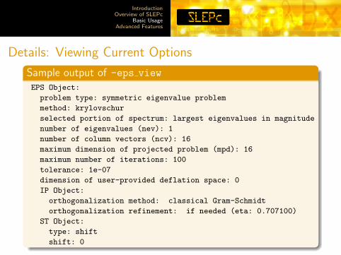
Sample output of -eps view
EPS Object:
problem type: symmetric eigenvalue problem
method: krylovschur
selected portion of spectrum: largest eigenvalues in magnitude
number of eigenvalues (nev): 1
number of column vectors (ncv): 16
maximum dimension of projected problem (mpd): 16
maximum number of iterations: 100
tolerance: 1e-07
dimension of user-provided deflation space: 0
IP Object:
orthogonalization method: classical Gram-Schmidt
orthogonalization refinement: if needed (eta: 0.707100)
ST Object:
type: shift
shift: 0

IntroductionOverview of SLEPc
Basic UsageAdvanced Features
EPS: Run-Time Examples
% program -eps_view -eps_monitor
% program -eps_type krylovschur -eps_nev 6 -eps_ncv 24
% program -eps_type arnoldi -eps_tol 1e-8 -eps_max_it 2000
% program -eps_type subspace -eps_hermitian -log_summary
% program -eps_type lapack
% program -eps_type arpack -eps_plot_eigs -draw_pause -1
% program -eps_type primme -eps_smallest_real

IntroductionOverview of SLEPc
Basic UsageAdvanced Features
Built-in Support Tools
I Plotting computed eigenvalues
% program -eps_plot_eigs
I Printing profiling information
% program -log_summary
I Debugging
% program -start_in_debugger% program -malloc_dump

IntroductionOverview of SLEPc
Basic UsageAdvanced Features
Built-in Support Tools
I Monitoring convergence(textually)
% program -eps_monitor
I Monitoring convergence(graphically)
% program -draw_pause 1-eps_monitor_draw

IntroductionOverview of SLEPc
Basic UsageAdvanced Features
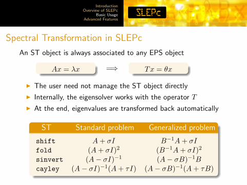
Spectral Transformation in SLEPc
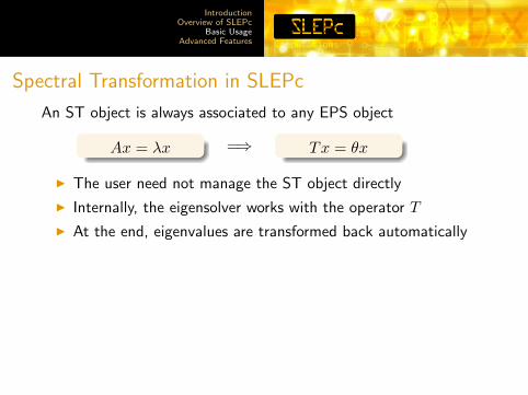
An ST object is always associated to any EPS object
Ax = λx =⇒ Tx = θx
I The user need not manage the ST object directly
I Internally, the eigensolver works with the operator T
I At the end, eigenvalues are transformed back automatically
ST Standard problem Generalized problem
shift A + σI B−1A + σIfold (A + σI)2 (B−1A + σI)2
sinvert (A− σI)−1 (A− σB)−1Bcayley (A− σI)−1(A + τI) (A− σB)−1(A + τB)
IntroductionOverview of SLEPc
Basic UsageAdvanced Features
Spectral Transformation in SLEPc
An ST object is always associated to any EPS object
Ax = λx =⇒ Tx = θx
I The user need not manage the ST object directly
I Internally, the eigensolver works with the operator T
I At the end, eigenvalues are transformed back automatically
ST Standard problem Generalized problem
shift A + σI B−1A + σIfold (A + σI)2 (B−1A + σI)2
sinvert (A− σI)−1 (A− σB)−1Bcayley (A− σI)−1(A + τI) (A− σB)−1(A + τB)

IntroductionOverview of SLEPc
Basic UsageAdvanced Features
Illustration of Spectral Transformation
Spectrum folding
θ
σ λλ1
θ1
λ2
θ2
λ3
θ3
θ=(λ−σ)2
Shift-and-invertθ
0 σ λλ1
θ1
λ2
θ2
θ= 1λ−σ
IntroductionOverview of SLEPc
Basic UsageAdvanced Features
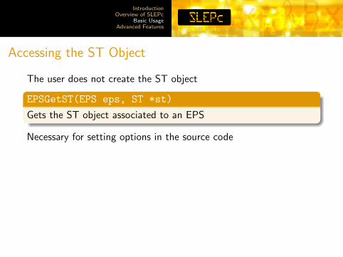
Accessing the ST Object
The user does not create the ST object
EPSGetST(EPS eps, ST *st)
Gets the ST object associated to an EPS
Necessary for setting options in the source code
Linear Solves. Most operators contain an inverse
I Linear solves are handled internally via a KSP object
STGetKSP(ST st, KSP *ksp)
Gets the KSP object associated to an ST
All KSP options are available, by prepending the -st prefix

IntroductionOverview of SLEPc
Basic UsageAdvanced Features
ST: Run-Time Examples
% program -eps_type power -st_type shift -st_shift 1.5
% program -eps_type power -st_type sinvert -st_shift 1.5
% program -eps_type power -st_type sinvert-eps_power_shift_type rayleigh
% program -eps_type arpack -eps_tol 1e-6-st_type sinvert -st_shift 1-st_ksp_type cgs -st_ksp_rtol 1e-8-st_pc_type sor -st_pc_sor_omega 1.3
IntroductionOverview of SLEPc
Basic UsageAdvanced Features
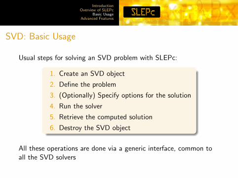
SVD: Basic Usage
Usual steps for solving an SVD problem with SLEPc:
1. Create an SVD object
2. Define the problem
3. (Optionally) Specify options for the solution
4. Run the solver
5. Retrieve the computed solution
6. Destroy the SVD object
All these operations are done via a generic interface, common toall the SVD solvers

IntroductionOverview of SLEPc
Basic UsageAdvanced Features
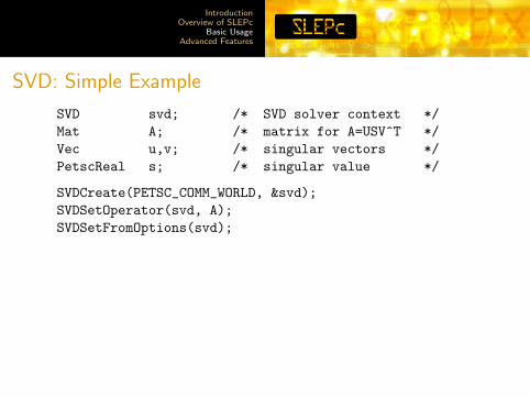
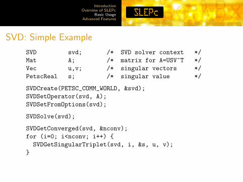
SVD: Simple Example
SVD svd; /* SVD solver context */Mat A; /* matrix for A=USV^T */Vec u,v; /* singular vectors */PetscReal s; /* singular value */
SVDCreate(PETSC_COMM_WORLD, &svd);SVDSetOperator(svd, A);SVDSetFromOptions(svd);
SVDSolve(svd);
SVDGetConverged(svd, &nconv);for (i=0; i<nconv; i++) {SVDGetSingularTriplet(svd, i, &s, u, v);
}
SVDDestroy(svd);
IntroductionOverview of SLEPc
Basic UsageAdvanced Features
SVD: Simple Example
SVD svd; /* SVD solver context */Mat A; /* matrix for A=USV^T */Vec u,v; /* singular vectors */PetscReal s; /* singular value */
SVDCreate(PETSC_COMM_WORLD, &svd);SVDSetOperator(svd, A);SVDSetFromOptions(svd);
SVDSolve(svd);
SVDGetConverged(svd, &nconv);for (i=0; i<nconv; i++) {SVDGetSingularTriplet(svd, i, &s, u, v);
}
SVDDestroy(svd);

IntroductionOverview of SLEPc
Basic UsageAdvanced Features
Details: Solving the Problem
SVDSolve(SVD svd)
Launches the SVD solver
Currently available SVD solvers:
I Cross-product matrix with any EPS eigensolver
I Cyclic matrix with any EPS eigensolver
I Golub-Kahan-Lanczos bidiagonalization with explicit restartand deflation
I Golub-Kahan-Lanczos bidiagonalization with thick restart anddeflation

IntroductionOverview of SLEPc
Basic UsageAdvanced Features
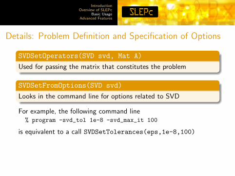
Details: Problem Definition and Specification of Options
SVDSetOperators(SVD svd, Mat A)
Used for passing the matrix that constitutes the problem
SVDSetFromOptions(SVD svd)
Looks in the command line for options related to SVD
For example, the following command line% program -svd_tol 1e-8 -svd_max_it 100
is equivalent to a call SVDSetTolerances(eps,1e-8,100)
SVDView(SVD svd, PetscViewer viewer)
Prints information about the object (equivalent to -svd view)
IntroductionOverview of SLEPc
Basic UsageAdvanced Features
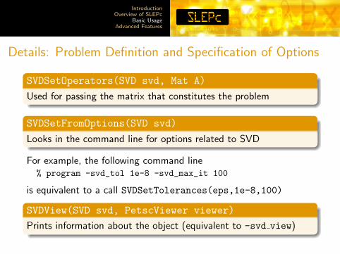
Details: Problem Definition and Specification of Options
SVDSetOperators(SVD svd, Mat A)
Used for passing the matrix that constitutes the problem
SVDSetFromOptions(SVD svd)
Looks in the command line for options related to SVD
For example, the following command line% program -svd_tol 1e-8 -svd_max_it 100
is equivalent to a call SVDSetTolerances(eps,1e-8,100)
SVDView(SVD svd, PetscViewer viewer)
Prints information about the object (equivalent to -svd view)
IntroductionOverview of SLEPc
Basic UsageAdvanced Features
Details: Problem Definition and Specification of Options
SVDSetOperators(SVD svd, Mat A)
Used for passing the matrix that constitutes the problem
SVDSetFromOptions(SVD svd)
Looks in the command line for options related to SVD
For example, the following command line% program -svd_tol 1e-8 -svd_max_it 100
is equivalent to a call SVDSetTolerances(eps,1e-8,100)
SVDView(SVD svd, PetscViewer viewer)
Prints information about the object (equivalent to -svd view)

IntroductionOverview of SLEPc
Basic UsageAdvanced Features
Details: Viewing Current Options
Sample output of -svd view
SVD Object:
method: trlanczos
transpose mode: explicit
selected portion of the spectrum: largest
number of singular values (nsv): 1
number of column vectors (ncv): 10
maximum dimension of projected problem (mpd): 10
maximum number of iterations: 100
tolerance: 1e-07
Lanczos reorthogonalization: two-side
IP Object:
orthogonalization method: classical Gram-Schmidt
orthogonalization refinement: if needed (eta: 0.707100)
IntroductionOverview of SLEPc
Basic UsageAdvanced Features
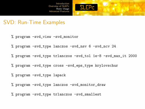
SVD: Run-Time Examples
% program -svd_view -svd_monitor
% program -svd_type lanczos -svd_nsv 6 -svd_ncv 24
% program -svd_type trlanczos -svd_tol 1e-8 -svd_max_it 2000
% program -svd_type cross -svd_eps_type krylovschur
% program -svd_type lapack
% program -svd_type lanczos -svd_monitor_draw
% program -svd_type trlanczos -svd_smallest

IntroductionOverview of SLEPc
Basic UsageAdvanced Features
Advanced Features

IntroductionOverview of SLEPc
Basic UsageAdvanced Features
Options for Subspace Generation
Initial Subspace
I Provide an initial trial subspace, e.g. from a previouscomputation
I Current support only for a single vector (EPSSetInitialVector)
Deflation Subspace
I Provide a deflation space with EPSAttachDeflationSpace
I The eigensolver operates in the restriction to the orthogonalcomplement
I Useful for constrained eigenproblems or problems with aknown nullspace
IntroductionOverview of SLEPc
Basic UsageAdvanced Features
Subspace Extraction
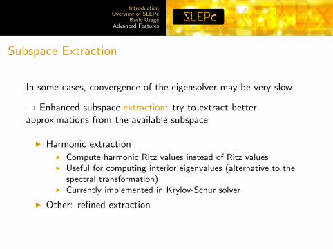
In some cases, convergence of the eigensolver may be very slow
→ Enhanced subspace extraction: try to extract betterapproximations from the available subspace
I Harmonic extractionI Compute harmonic Ritz values instead of Ritz valuesI Useful for computing interior eigenvalues (alternative to the
spectral transformation)I Currently implemented in Krylov-Schur solver
I Other: refined extraction

IntroductionOverview of SLEPc
Basic UsageAdvanced Features
Computation of Many Eigenpairs
By default, a subspace of dimension 2 · nev is used...For large nev, this is not appropriate
I Excessive storage and inefficient computation
A Vm = Vm
Sm
b∗m+1
Strategy: compute eigenvalues in chunks - restrict the dimensionof the projected problem
% program -eps_nev 2000 -eps_mpd 300
IntroductionOverview of SLEPc
Basic UsageAdvanced Features
SLEPc Highlights
I Growing number of eigensolvers
I Seamlessly integrated spectral transformation
I Support for SVD
I Easy programming with PETSc’s object-oriented style
I Data-structure neutral implementation
I Run-time flexibility, giving full control over the solutionprocess
I Portability to a wide range of parallel platforms
I Usable from code written in C, C++ and Fortran
I Extensive documentation

IntroductionOverview of SLEPc
Basic UsageAdvanced Features
Future Directions
Under Development
I Generalized Davidson and Jacobi-Davidson solvers
I Enable computational intervals for symmetric problems
Mid Term
I Conjugate Gradient-type eigensolvers
I Non-symmetric Lanczos eigensolver
I Support for other types of eigenproblems: quadratic,structured, non-linear
IntroductionOverview of SLEPc
Basic UsageAdvanced Features
More Information
Homepage:http://www.grycap.upv.es/slepc
Hands-on Exercises:http://www.grycap.upv.es/slepc/handson
Contact email:[email protected]