JHEP12(2013)009

Published for SISSA by Springer

Received: September 27, 2013

Accepted: November 22, 2013

Published: December 2, 2013

Left-handed Z′ and Z FCNC quark couplings facing

new b→ sµ+µ− data

Andrzej J. Buras and Jennifer Girrbach

TUM-IAS, Lichtenbergstr. 2a, D-85748 Garching, Germany

Physik Department, TUM, D-85748 Garching, Germany

E-mail: andrzej.buras@tum.de, jennifer.girrbach@tum.de

Abstract: In view of the recent improved data on Bs,d → µ+µ− and Bd → K∗µ+µ− we

revisit two simple New Physics (NP) scenarios analyzed by us last year in which new FCNC

currents in b → sµ+µ− transitions are mediated either entirely by a neutral heavy gauge

boson Z ′ with purely left-handed complex couplings ∆qbL (Z ′) (q = d, s) and real couplings

to muons ∆µµA (Z ′) and ∆µµ

V (Z ′) or the SM Z boson with left-handed complex couplings

∆qbL (Z). We demonstrate how the reduced couplings, the couplings in question divided by

MZ′ or MZ , can be determined by future ∆F = 2 and b→ sµ+µ− observables up to sign

ambiguities. The latter do not affect the correlations between various observables that can

test these NP scenarios. We present the results as functions of CBq = ∆Mq/(∆Mq)SM, Sψφand SψKS

which should be precisely determined in this decade. We calculate the violation

of the CMFV relation between B(Bs,d → µ+µ−) and ∆Ms,d in these scenarios. We find

that the data on Bs,d → µ+µ− from CMS and LHCb can be reproduced in both scenarios

but in the case of Z, ∆Ms and Sψφ have to be very close to their SM values. As far

as Bd → K∗µ+µ− anomalies are concerned the Z ′ scenario can significantly soften these

anomalies while the Z boson fails badly because of the small vector coupling to muons.

We also point out that recent proposals of explaining these anomalies with the help of a

real Wilson coefficient CNP9 implies uniquely an enhancement of ∆Ms with respect to its

SM value, while a complex CNP9 allows for both enhancement and suppression of ∆Ms and

simultaneously novel CP-violating effects. Correlations between b → sµ+µ− and b → sνν

observables in these scenarios are emphasized. We also discuss briefly scenarios in which

the Z ′ boson has right-handed FCNC couplings. In this context we point out a number

of correlations between angular observables measured in Bd → K∗µ+µ− that arise in the

absence of new CP-violating phases in scenarios with only left-handed or right-handed

couplings or scenarios in which left-handed and right-handed couplings are equal to each

other or differ by sign.

Keywords: Beyond Standard Model, B-Physics

ArXiv ePrint: 1309.2466

c© SISSA 2013 doi:10.1007/JHEP12(2013)009

JHEP12(2013)009

Contents

1 Introduction 1

2 Basic formulae 6

2.1 Basic Lagrangian 6

2.2 ∆F = 2 observables 7

2.3 b→ sµ+µ− observables 7

2.4 Correlations between ∆Ms,d, Bs,d → µ+µ− and CNP9 10

3 Determining the parameters in the LHS 12

4 Correlations between flavour observables in the LHS 14

4.1 Preliminaries 14

4.2 Strategy 15

4.3 Performing steps 1 and 2 16

4.4 Performing step 3 18

4.5 The b→ sνν Transitions 24

4.6 Comments on other NP models 25

5 The case of the SM Z 26

6 Comments on a real CNP9 and right-handed couplings 29

6.1 Real CNP9 29

6.2 Right-handed currents 30

7 Conclusions and outlook 39

A General formulae for correlations 41

1 Introduction

The correlations between flavour observables in concrete New Physics (NP) models are

a powerful tool to distinguish between various models and to select the ones that are

consistent with the data [1]. Among prominent examples where such correlations are rather

stringent are models with constrained minimal flavour violation (CMFV) [2, 3], MFV at

large [4–6], GMFV [7], models with U(2)3 flavour symmetry [8–11] and supersymmetric

models with flavour symmetries [12].

Also models in which all FCNCs are mediated entirely by a neutral have gauge boson

Z ′ imply a multitude of correlations as analyzed in detail in [13–17]. A review of Z ′ models

can be found in [18] and other recent studies in these models have been presented in [19–24].

– 1 –

JHEP12(2013)009

While FCNC Z ′ couplings to quarks could be generally left-handed and right-handed,

as demonstrated in particular in [14], a very interesting scenario is the LHS one in which

Z ′ couplings to quarks are purely left-handed. The nice virtue of this scenario is that

for certain choices of the Z ′ couplings the model resembles the structure of CMFV or

models with U(2)3 flavour symmetry. Moreover as no new operators beyond those present

in the SM are present, the non-perturbative uncertainties are the same as in the SM, still

allowing for non-MFV contributions beyond those present in U(2)3 models. In particular

the stringent CMFV relation between ∆Ms,d and B(Bs,d → µ+µ−) [25] valid in the simplest

U(2)3 models is violated in the LHS scenario as we will see below.

Another virtue of the LHS scenario is the paucity of its parameters that enter all flavour

observables in a given meson system which should be contrasted with most NP scenarios

outside the MFV framework. Indeed, if we concentrate on B0s − B0

s mixing, b → sµ+µ−

and b → sνν observables there are only four new parameters to our disposal: the three

reduced couplings of which the first one is generally complex and the other two real. These

are (our normalizations of couplings are given in section 2)

∆sbL (Z ′) =

∆sbL (Z ′)

MZ′, ∆µµ

A (Z ′) =∆µµA (Z ′)

MZ′, ∆µµ

V (Z ′) =∆µµV (Z ′)

MZ′, (1.1)

where the bar distinguishes these couplings from the ones used in [14]. The couplings

∆µµA,V (Z ′) are defined in (2.4) and due to SU(2)L symmetry implying in LHS ∆νν

L (Z ′) =

∆µµL (Z ′) one also has

∆ννL (Z ′) =

∆µµV (Z ′)−∆µµ

A (Z ′)

2. (1.2)

Concrete models satisfying this relation are the 3-3-1 models analyzed in [13]. This relation

has also been emphasized recently in [26, 27].

The four new parameters in (1.1) describe in this model NP effects in flavour violating

processes, in particular

∆Ms, Sψφ, Bs → µ+µ−, Ssµµ, B → Kνν, B → K∗νν, B → Xsνν. (1.3)

and

Bd → Kµ+µ−, Bd → K∗µ+µ−, Bd → Xsµ+µ−. (1.4)

Extending these considerations to B0d − B0

d mixing and Bd → µ+µ− we have to our

disposal presently

∆Md, SψKS, Bd → µ+µ−. (1.5)

It should be noted that in these three observables only ∆dbL (Z ′) is new as the muon couplings

∆µµA,V (Z ′) are already determined through the observables (1.3) and (1.4).

In [14] a very detailed analysis of the correlations among observables in (1.3) and

among the ones in (1.5) has been presented taking into account the constraints from the

processes (1.4) known at the time of our analysis. In the meantime two advances on the

experimental side have been made that deal with processes listed above:

– 2 –

JHEP12(2013)009

• The LHCb and CMS collaborations presented new results on Bs,d → µ+µ− [28–

30]. While the branching ratio for Bs → µ+µ− turns out to be rather close to SM

prediction, although a bit lower, the central value for the one of Bd → µ+µ− is by a

factor of 3.5 higher than its SM value.

• LHCb collaboration reported new results on angular observables in Bd → K∗µ+µ−

that show significant departures from SM expectations [31, 32]. Moreover, new data

on the observable FL, consistent with LHCb value in [31] have been presented by

CMS [33].

In particular the anomalies in Bd → K∗µ+µ− triggered recently two sophisticated analy-

ses [26, 34] with the goal to understand the data and to indicate what type of new physics

could be responsible for these departures from the SM. Both analyses point toward NP

contributions in the modified coefficients C7γ and C9 with the following shifts with respect

to their SM values:

CNP7γ < 0, CNP

9 < 0. (1.6)

Other possibilities, in particular involving right-handed currents, have been discussed

in [26]. It should be emphasized at this point that these analyses are subject to theo-

retical uncertainties, which have been discussed at length in [34–38] and it remains to be

seen whether the observed anomalies are only result of statistical fluctuations and/or un-

derestimated error uncertainties. Assuming that this is not the case we will investigate

how LHS faces these data.

As far as CNP9 is concerned, the favorite scenario suggested in [34] is precisely the LHS

scenario analyzed in [14] but with a simplifying assumption that CNP9 is real. In [34] it

has also been suggested that ∆µµA (Z ′) ≈ 0 and in fact also in the examples of Z ′ models

presented in [26, 27] the axial-vector coupling has been set to zero. Clearly such a solution,

as already mentioned in these papers, would eliminate NP contributions to Bs → µ+µ−

which although consistent with the present data is not particularly interesting. We would

like to add that such a choice would also eliminate NP contributions to Bd → µ+µ−

precluding the explanation in LHS of a possible enhancement of B(Bd → µ+µ−) indicated

by the LHCb and CMS data.

It should be remarked that according to the analysis in [26] CNP9 , while reducing

significantly the anomalies in the angular observables S5 and FL, cannot provide a complete

solution when the data on B → Kµ+µ− and the forward-backward asymmetry AFB are

taken into account. Yet the nice pattern that a negative CNP9 automatically shifts S5 and

FL in the right direction towards the data is a virtue of this simple scenario.

The inclusion of a negative NP contribution CNP7γ , which exhibits the same pattern in

the shifts in S5 and FL, together with CNP9 would provide a better fit to the data. However

in the context of our general analysis in [14] we have demonstrated that the contribution

of Z ′ to C7γ is fully negligible. Whether this is a problem for LHS remains to be seen when

the data on Bd → K∗µ+µ− and B → Xsγ improve. Thus indeed in what follows we can

concentrate on modifications in two Wilson coefficients, C9 and C10, that are relevant for

flavour observables in Bd → K∗µ+µ− and Bs → µ+µ−, respectively.

– 3 –

JHEP12(2013)009

Having developed the full machinery for analyzing the processes in question in Z ′

models in [14] we would like in this paper to have still another look at the LHS scenario

in view of the most recent data. As already two detailed analyses of anomalies in Bd →K∗µ+µ− have been presented in [26, 34], our paper will be dominated by Bs,d → µ+µ−

decays. Therefore, in contrast to these papers the vector-axial coupling ∆µµA (Z ′) will play

a crucial role in our analysis. In particular in the spirit of [1, 14] we will expose in the

LHS the correlations between ∆F = 2 observables and Bs,d → µ+µ− illustrating their

dependence on ∆Ms,d/(∆Ms,d)SM, Sψφ and SψKSwhich should be precisely determined in

this decade. Here the theoretically clean CMFV relation between these observables [25],

that is violated in the LHS, will play a prominent role. However, we will also briefly

discuss the correlation between ∆Ms and the size of CNP9 necessary to understand the

Bd → K∗µ+µ− anomalies [26, 34].

Now, in [14] we have performed already a very detailed analysis of the processes and

observables listed in (1.3) and (1.5) in the LHS scenario and it is mandatory for us to state

what is new in the present paper:

• First of all the data on Bs,d → µ−µ− changed relative to those known at the time of

the analysis in [14] and we would like to confront LHS with these data. In particular

as stated above we will calculate the deviations from the stringent CMFV relation

between ∆Ms,d and B(Bs,d → µ+µ−) [25] present in this model that has not been

done in [14] nor in any other paper known to us. An exception is our analysis of 3-3-1

models in [13] but in this concrete Z ′ model NP effects in Bd → µ+µ− are too small

to reproduce the recent data within 1σ.

• While in [14] we have demonstrated how the coupling ∆sbL (Z ′) could be determined

from ∆Ms, Sψφ and Bs → µ+µ− observables and the coupling ∆dbL (Z ′) from ∆Md,

SψKSand Bd → µ+µ−, we have done it for chosen values of the muon coupling

∆µµA (Z ′) and MZ′ and using in particular the CP-asymmetry Ssµµ which is very diffi-

cult to measure. In the present paper we want to summarize how the three reduced

couplings listed in (1.1) can be determined by invoking in addition the angular ob-

servables in Bd → K∗µ+µ− that can be much easier measured than Ssµµ and not

making a priori any assumptions on ∆µµA,V (Z ′) and MZ′

• In view of the continued progress in lattice calculations we will investigate how the

results presented here depend on the values of CBs and CBdwhose departure from

unity measures the NP effects in ∆Ms and ∆Md. We will see that precise knowledge

of these parameters as well as precise measurements of CP-asymmetries Sψφ and

SψKSare very important for the determination of the couplings in (1.1).

• We will refine our previous analysis of the correlations of Bs → µ+µ− and b → sνν

observables.

• In the context of our presentation we will critically analyze the LHS scenario with

a real coefficient CNP9 advocated in [26, 34]. In particular we present a correlation

between real CNP9 and ∆Ms pointing out that in LHS ∆Ms is then uniquely enhanced

– 4 –

JHEP12(2013)009

which could be tested one day when lattice calculations and values of CKM param-

eters will be more precise. We discuss briefly the implications of such a scenario for

Bs → µ+µ−, Sψφ and b→ sνν transitions.

• We point out a number of correlations between angular observables in Bd → K∗µ+µ−

which arise in LHS, RHS, LRS and ALRS scenarios for couplings of [14] when new

CP-violating phases are neglected.

• As far as Z-scenario is concerned we note that large enhancement of B(Bd → µ+µ−)

found by us in [14] is fully consistent with the recent LHCb and CMS data. However,

this scenario does not allow the explanation of the Bd → K∗µ+µ− anomalies when

the constraint from ∆Ms is taken into account. Due to the smallness of the vector

coupling of Z to muons the required modification of C9 implies in this scenario shifts

in ∆Ms and in C10 that are by far too large.

Our paper is organized as follows. In section 2 we summarize the basic formulae used

in our analysis referring often to the expressions in [14], where the same notation is used.

In section 3 we show a simple procedure for the determination of the reduced couplings

in (1.1) up to their signs. In section 4, the most important section of our paper, we

perform an anatomy of correlations between B0s,d − B0

s,d and Bs,d → µ+µ− observables

taking into account the information from Bd → K∗µ+µ− decay. We also include b→ sνν

in this discussion. In section 5 we consider the case of the SM Z gauge boson with FCNC

couplings. In this case the leptonic reduced couplings are fixed. In section 6 we address the

case of a real C9, the enhancement of ∆Ms in this case and of the implications for other

observables. We also discuss briefly scenarios in which Z ′ and Z have also right-handed

FCNC couplings and point out a number of correlations between angular observables in

Bd → K∗µ+µ− advertised above. We conclude in section 7.

Before starting our presentation let us realize that the challenges the LHS scenario

considered in our paper has to face are non-trivial due to the following facts.

The important actors in our paper are the couplings

∆sbL (Z ′), ∆db

L (Z ′), ∆µµA (Z ′), ∆µµ

V (Z ′), (1.7)

in terms of which the decays and related observables in (1.3)–(1.5) should be simultaneously

described. In view of the pattern of the present data mentioned above this is certainly non-

trivial for the following reasons:

• ∆sbL (Z ′) enters both Bs → µ+µ− and Bd → K∗µ+µ− in which NP effects have been

found to be small and sizable, respectively. This implies through the relation (2.17)

that ∆µµA (Z ′) < ∆µµ

V (Z ′).

• The smallness of ∆sbL (Z ′) is welcome as then also NP effects in ∆Ms are small as

seen in the data. But then ∆µµV (Z ′) must be sufficiently large in order to describe

the anomalies in Bd → K∗µ+µ−.

– 5 –

JHEP12(2013)009

• Similarly ∆µµA (Z ′) cannot be small, in spite of Bs → µ+µ− being SM-like as otherwise

the enhancement ofBd → µ+µ− branching ratio over SM expectation indicated by the

LHCb and CMS data cannot be accommodated. Here the sizable coupling ∆dbL (Z ′)

could help, but it is constrained by ∆Md and SψKS.

• In the Z-scenario the challenges are even larger as the lepton couplings are fixed.

We are now ready to investigate how LHS Z ′ and Z scenarios face these challenges.

2 Basic formulae

2.1 Basic Lagrangian

The basic formalism for our analysis has been developed in [14] and we collect here only

those formulae of that paper that are essential for our presentation expressing them this

time in terms of the reduced couplings in (1.1). However we recall first the basic Lagrangian

in terms of the couplings used in [14] (q = d, s):

LquarksFCNC(Z ′) =

[qγµPLb∆

qbL (Z ′) + qγµPRb∆

qbR (Z ′) + h.c.

]Z ′µ, (2.1)

Lleptons(Z ′) =[µγµPLµ∆µµ

L (Z ′) + µγµPRµ∆µµR (Z ′) + νγµPL∆νν

L (Z ′)]Z ′µ (2.2)

where R and L stand for right-handed and left-handed couplings γµ(1± γ5)/2. Moreover

∆bqL (Z ′) =

[∆qbL (Z ′)

]∗(2.3)

and the vector and axial-vector couplings to muons are given as follows

∆µµV (Z ′) = ∆µµ

R (Z ′) + ∆µµL (Z ′),

∆µµA (Z ′) = ∆µµ

R (Z ′)−∆µµL (Z ′).

(2.4)

The relation of these couplings to the ones used in [26] is as follows

∆qbL,R(Z ′) =

g2

2 cos θWgL,Rqb , ∆µµ

V,A(Z ′) =g2

cos θWgV,Aµ , (2.5)

where g2 is the SU(2)L gauge coupling. For completeness and because of a brief discussion

in section 6 we have included here right-handed couplings ∆qbR (Z ′) which vanish in the LHS.

On the other hand we do not make any assumptions about diagonal couplings of Z ′

to quarks but we expect them to be non-vanishing. The flavour violating couplings in

the quark mass eigenstate basis can e.g. arise from the non-universality of the diagonal

couplings in the flavour basis but other dynamical mechanisms for the FCNC couplings

in question are possible [18]. Without a concrete model it is not possible to establish a

relation between diagonal and non-diagonal couplings. For a recent discussion see [39] and

references therein.

– 6 –

JHEP12(2013)009

2.2 ∆F = 2 observables

The B0s − B0

s observables are fully described in LHS by the function

S(Bs) = S0(xt) + ∆S(Bs) ≡ |S(Bs)|e−i2ϕBs , (2.6)

where S0(xt) is the real one-loop SM box function and the additional generally complex

term, denoted in [14] by [∆S(Bs)]VLL, is the tree-level Z ′ contribution

∆S(Bs) =

[∆bsL (Z ′)

V ∗tbVts

]24r

g2SM

, g2SM = 4

GF√2

α

2π sin2 θW. (2.7)

Here r is a QCD factor that includes QCD renormalization group effects between µ = MZ′

and µ = mt and the difference in matching conditions between full and effective theories

in the tree-level Z ′ exchanges [40] and SM box diagrams [41]. Explicit expression for r has

been given in [13]. One finds r = 0.985, r = 0.953 and r = 0.925 for MZ′ = 1, 3, 10 TeV,

respectively.

The two observables of interest, ∆Ms and Sψφ are then given by

∆Ms =G2F

6π2M2WmBs |V ∗tbVts|2F 2

BsBBsηB|S(Bs)| (2.8)

and

Sψφ = sin(2|βs| − 2ϕBs) , Vts = −|Vts|e−iβs . (2.9)

with βs ' −1◦ .

In the case of B0d system the corresponding formulae are obtained from (2.6)–(2.8) by

replacing s by d. Moreover (2.9) is replaced by

SψKS= sin(2β − 2ϕBd

) , Vtd = |Vtd|e−iβ. (2.10)

The value of β depends strongly on |Vub| but only weakly on its phase γ. For γ = 68◦ we

find β = 21.2◦ and β = 25.2◦ for |Vub| = 3.4× 10−3 and |Vub| = 4.0× 10−3, respectively.

It should be noted that MZ′ is hidden in the reduced Z ′bs coupling and appears

explicitly only in r but this dependence is only logarithmic and can be neglected in view

of present theoretical and experimental uncertainties but should be taken into account in

the flavour precision era. However, except for this weak dependence at tree level it is

not possible to measure MZ′ through FCNC processes unless the relevant couplings are

predicted in a given model. On the other hand it could be in principle possible through

loop processes one day or through direct high energy experiments that would discover Z ′.

2.3 b→ sµ+µ− observables

The two Wilson coefficients that receive NP contributions in LHS model are C9 and C10.

We decompose them into the SM and NP contributions:1

C9 = CSM9 + CNP

9 , C10 = CSM10 + CNP

10 . (2.11)

1These coefficients are defined as in [14] and the same definitions are used in [26, 34].

– 7 –

JHEP12(2013)009

Then [14]2

sin2 θWCSM9 = sin2 θWP

NDR0 + [ηY Y0(xt)− 4 sin2 θWZ0(xt)], (2.12)

sin2 θWCSM10 = −ηY Y0(xt) (2.13)

so that

CSM9 ≈ 4.1, CSM

10 ≈ −4.1 . (2.14)

NP contributions have a very simple structure

sin2 θWCNP9 = − 1

g2SM

∆sbL (Z ′)∆µµ

V (Z ′)

V ∗tsVtb, (2.15)

sin2 θWCNP10 = − 1

g2SM

∆sbL (Z ′)∆µµ

A (Z ′)

V ∗tsVtb. (2.16)

and consequently we have an important relation

CNP10

CNP9

=∆µµA (Z ′)

∆µµV (Z ′)

, (2.17)

which involves only leptonic couplings.

Y0(xt) and Z0(xt) are SM one-loop functions, analogous to S0(xt). Explicit expressions

for them can be found in [14]. C10 is scale independent as far as pure QCD corrections are

concerned but at higher order in QED the relevant operator mixes with other operators [42,

43]. This effect will be included in the complete calculation of NLO electroweak corrections

to Bs → µ+µ−. C9 is affected by QCD corrections, present in the term PNDR0 , through

mixing with four-quark current-current operators. Its value is usually quoted at µ = O(mb).

Beyond one-loop this term is renormalization scheme dependent but as demonstrated in [44]

at the NLO level this dependence is canceled by QCD corrections to the matrix elements of

the relevant operators. By now these corrections are known at the NNLO level [42, 45, 46]

and are taken into account in the extraction of CNP9 from the data. Finally, it should be

mentioned that there are also QCD corrections affecting the NP part due to the mixing

of new four-quark operators generated through Z ′ exchange. These corrections would

effectively modify the term PNDR0 . Corrections of this type have been calculated in the

case of Z ′ contributions to B → Xsγ decay in [14, 47] and found to be small. As the

anomalous dimensions in the present case are smaller than in the case of B → Xsγ it is

safe to neglect these corrections.

One has then in the case of Bs → µ+µ− decay [16, 48, 49]

B(Bs → µ+µ−)

B(Bs → µ+µ−)SM

=

[1 +Aµµ∆Γ ys

1 + ys

]|P |2, P =

C10

CSM10

≡ |P |eiϕP , (2.18)

where

Aµµ∆Γ = cos(2ϕP − 2ϕBs), ys ≡ τBs

∆Γs2

= 0.088± 0.014. (2.19)

2The quantities ηY , ηB and ηX appearing in the text are QCD corrections for which the values, all O(1),

can be found in [14].

– 8 –

JHEP12(2013)009

The bar indicates that ∆Γs effects have been taken into account. In the SM and CMFV

Aµµ∆Γ = 1 but in the LHS it is slightly smaller and we take this effect into account. Generally

as shown in [16] Aµµ∆Γ can serve to test NP models as it can be determined in time-dependent

measurements [48, 49]. Of interest is also the CP asymmetry

Ssµµ = sin(2ϕP − 2ϕBs), (2.20)

which has been studied in detail in [14, 16] in the context of Z ′ models.

In the case of Bd → µ+µ− decay the formulae given above apply with s replaced

by d and yd ≈ 0. While CSM10 remains unchanged, CNP

10 is clearly modified through the

replacement of Vts by Vtd and different Z ′ coupling to quarks. But the muon coupling

remains unchanged and this will allow a correlation between Bs → µ+µ− and Bd → µ+µ−

which will be investigated within LHS here for the first time. Explicit formulae for Bd →µ+µ− can be found in [14].

Concerning the status of the branching ratios for Bs,d → µ+µ− decays we have

B(Bs → µ+µ−)SM = (3.56± 0.18) · 10−9, B(Bs → µ+µ−) = (2.9± 0.7)×10−9, (2.21)

B(Bd → µ+µ−)SM = (1.05± 0.07)× 10−10, B(Bd → µ+µ−) =(3.6+1.6−1.4

)× 10−10, (2.22)

where the SM values are based on [16, 50] and experimental data are the most recent

average of the results from LHCb and CMS [28–30].

In the case of B → K∗µ+µ− we will concentrate our discussion on the Wilson coefficient

CNP9 which can be extracted from the angular observables, in particular 〈FL〉, 〈S5〉 and 〈A8〉,

in which within the LHS NP contributions enter exclusively through this coefficient. On

the other hand Im(CNP10 ) governs the CP-asymmetry 〈A7〉. Useful approximate expressions

for these four angular observables in terms of CNP9 and CNP

10 have been provided in [26].

The recent B → K∗µ+µ− anomalies imply the following ranges for CNP9 (Bs) [26, 34]

respectively

CNP9 (Bs) = −(1.6± 0.3), CNP

9 (Bs) = −(0.8± 0.3) (2.23)

As CSM9 (Bs) ≈ 4.1 at µb = 4.8 GeV, these are very significant suppressions of this coef-

ficient. We note that C9 remains real as in the SM. We will have a closer look at the

implications of this result for both values quoted above. The details behind these two

results that differ by a factor of two is discussed in [26]. In fact inspecting figures 3 and 4

of the latter paper one sees that if the constraints from AFB and B → Kµ+µ− were not

taken into account CNP9 (Bs) ≈ −1.4 could alone explain the anomalies in the observables

FL and S5. But the inclusion of these constraints reduces the size of this coefficient. Yet

values of CNP9 (Bs) ≈ −(1.2− 1.0) seem to give reasonable agreement with all data and the

slight reduction of departure of FL and S5 from their SM values in the future data would

allow to explain the two anomalies with the help of CNP9 (Bs) as suggested originally in [34].

Similarly a very recent comprehensive Bayesian analysis of the authors of [51, 52]

in [53], that appeared after our analysis, finds that although SM works well, if one wants

to interpret the data in extensions of the SM then NP scenarios with dominant NP effect in

C9 are favoured although the inclusion of chirality-flipped operators in agreement with [26]

– 9 –

JHEP12(2013)009

would help to reproduce the data. This is also confirmed in our paper and in the very

recent paper in in [54]. References to earlier papers on B → K∗µ+µ− by all these authors

can be found in [26, 34, 52] and [1].

We are looking forward to the analysis of the authors of [51, 52] in order to see whether

some consensus about the size of anomalies in question between these three groups has been

reached.

2.4 Correlations between ∆Ms,d, Bs,d → µ+µ− and CNP9

In [14] a number of correlations between ∆F = 2 and ∆F = 1 observables in LHS have been

identified. Here we want to concentrate on the correlations between ∆Ms,d, Bs,d → µ+µ−

and CNP9 as they can be exposed analytically.

First the CMFV relation between B(Bq → µ+µ−) and ∆Ms,d [25] generalizes in LHS

to (q = s, d)

B(Bq → µ+µ−) = CτBq

Bq

|Y qA|2

|S(Bq)|∆Mq, (2.24)

with C = 6πη2Y

η2B

(α

4π sin2 θW

)2 m2µ

M2W

= 4.395 · 10−10, (2.25)

S(Bq) given in (2.6) and

Y qA = ηY Y0(xt) +

∆qbL (Z ′)

VtbV∗tq

[∆µµA (Z ′)

]M2Z′g2

SM

. (2.26)

Note that these relations are free from FBq dependence but in contrast to CMFV they

depend on Vtq as generally ∆qbL (Z ′) are not aligned with VtbV

∗tq. The main uncertainty in

these relations comes from the parameters Bq that are known presently with an accuracy

of ±8% and ±4.5% for Bd and Bs, respectively (see new version of FLAG [55]). More

accurate is the relation [25]

B(Bs → µ+µ−)

B(Bd → µ+µ−)=Bd

Bs

τ(Bs)

τ(Bd)

∆Ms

∆Mdr, r =

∣∣∣∣Y sA

Y dA

∣∣∣∣2 ∣∣∣∣S(Bd)

S(Bs)

∣∣∣∣ , Bd

Bs= 0.99±0.02 (2.27)

where the departure of r from unity measures effects which go beyond CMFV. Still as shown

already in [25] in the context of supersymmetric models with MFV and in the context of

GMFV in [7] at large tanβ one also finds r ≈ 1 so that this relation offers also a test of

these scenarios. On the other hand the most general test of MFV, as emphasized in [56],

is the proportionality of the ratio of the two branching ratios in question to |Vts|2/|Vtd|2.

It should be noted that in (2.27) the only theoretical uncertainty enters through the

ratio Bs/Bd that is already now known from lattice calculations with impressive accuracy of

roughly ±2% [57] as given in (2.27).3 Therefore the relation (2.27) should allow a precision

test of CMFV, related scenarios mentioned above and LHS even if the branching ratios

B(Bs,d → µ+µ−) would turn out to deviate from SM predictions only by 10 − 15%. We

3This result is not included in the recent FLAG update which quotes 0.95± 0.10.

– 10 –

JHEP12(2013)009

should emphasize that such a precision test is not possible with any angular observable

in Bd → K∗µ+µ− due to form factor uncertainties. On the other hand these observables

provide more information on NP than the relation (2.27).

In fact as seen in figure 9 the present data for r differ from its CMFV value (r = 1)

by more than a factor of four

rexp = 0.23± 0.11. (2.28)

Even if in view of large experimental uncertainties one cannot claim that here NP is at

work, this plot invites us to investigate whether LHS could cope with the future more

precise experimental results in which the central values of the branching ratios in (2.21)

and (2.22) would not change by much.

As far as the Wilson coefficients CNP9 and CNP

10 are concerned we have two important

relations

(∆S)∗ = 4rg2SM sin4 θW

[CNP

9

∆µµV (Z ′)

]2

= 0.037

[CNP

9

∆µµV (Z ′)

]2 [MZ′

1 TeV

]2

, (2.29)

(∆S)∗ = 4rg2SM sin4 θW

[CNP

10

∆µµA (Z ′)

]2

= 0.037

[CNP

10

∆µµA (Z ′)

]2 [MZ′

1 TeV

]2

, (2.30)

which we have written in a form suitable for the analysis in section 6. We recall that

SSM = S0(xt) = 2.31.

These relations can be derived from (2.7), (2.15) and (2.16). The last relation, already

encoded in previous relations, has been extensively studied in [14] for fixed value of the

coupling ∆µµA (Z ′). It is evident that independently of the sign of this coupling in the case

of a real CNP10 , ∆S and ∆Ms will be enhanced which with the lattice value

√BBsFBs =

(279 ± 13) MeV [58] used in [14] would be a problem [59]. Making CNP10 complex allowed

through destructive interference with the SM contribution to lower the value of ∆Ms and

bring it to agree with the data. With the new value for

√BBsFBs MeV given below this

problem is softened.

Concerning (2.29), we note that in the case of a real CNP10 , the relation (2.17) implies

that also CNP9 must be real in LHS so that also this relation implies in this case uniquely

an enhancement of ∆S and ∆Ms.

In the next section we will get an idea on the range of the values of ∆µµA (Z ′) by

looking simultaneously at Bs → µ+µ− and Bd → µ+µ− decays. In the case of ∆µµV (Z ′)

the simultaneous consideration of the decays Bd → K∗µ+µ− and Bd → ρµ+µ− could give

us in principle information about the size of this coupling. However, there is not enough

experimental information on the latter decay and such an exercise cannot be performed at

present.

On the other hand in the context of (2.29) it has been noted in [27] that ∆µµV (Z ′)

could be eliminated in favour of the violation of the CKM unitarity in Z ′ models studied

by Marciano and Sirlin long time ago [60] if one assumes that ∆sbA = 0 and the diagonal

couplings of Z ′ to quarks vanish. As already admitted by the authors of [27] such a model

– 11 –

JHEP12(2013)009

is not realistic. Therefore we provide here a more general formula which uses the results

in [60] without making the assumptions made in [27].

We denote the violation of CKM unitarity by

∆CKM = 1−∑

q=d,s,b

|Vuq|2 = −∆CKM, (2.31)

with ∆CKM used in [27, 60]. Then for MZ′ �MW we find

∆CKM =3√

2

8GF

α

π sin2 θW∆µµL (Z ′)

(∆µµL (Z ′)− ∆dd

L (Z ′))

lnM2Z′

M2W

, (2.32)

where ∆ddL is the diagonal coupling of Z ′ to down-quarks which is assumed to be generation

independent.

The triple correlation between ∆Ms, ∆CKM and CNP9 found in [27] only follows for the

case

∆µµV (Z ′) =

∆µµL (Z ′)

2, ∆dd

L (Z ′) = 0, (2.33)

where the first equality is equivalent to ∆µµA (Z ′) = 0. The triple correlation in question

can now be rewritten as

(∆S)∗ ∆CKM =3

4r(απ

)2(CNP

9 )2 lnM2Z′

M2W

, (2.34)

which allows better to follow the signs than the expression given by these authors. As now

∆CKM ≥ 0, it is evident also from this formula that in the case of a real CNP9 , independently

of its sign, ∆S is real and strictly positive enhancing uniquely ∆Ms. In [27] only |∆S| has

been studied.

However, generally the assumptions in (2.33) are violated and in examples shown in [60]

there is always a quark contribution to ∆CKM. In fact these authors present GUT examples

where the quark contribution cancels the one of leptons so that in such a model there is

no violation of CKM unitarity.

Independently of this discussion the case of a real CNP9 is interesting in itself and in

section 6 we will investigate how the predictions of the LHS model would look like in

the presence of a real CNP9 as large as required to remove the anomalies in the data on

Bd → K∗µ+µ−.

3 Determining the parameters in the LHS

In principle there are many ways to bound or even determine the reduced parameters

in (1.1). Here we present one route which simultaneously allows already at the early stage

to test the LHS. This route could be improved and modified dependently on evolution of

experimental data.

To this end we use the parametrization

∆sbL (Z ′) = −|∆sb

L (Z ′)|eiδ23 , |∆sbL (Z ′)| = s23

MZ′, (3.1)

– 12 –

JHEP12(2013)009

where s23 and δ23 are parameters used in [14] and the minus sign is introduced to cancel

the minus sign in Vts in the relevant phenomenological formulae. For Bd − B0d mixing and

Bd → µ+µ− s is replaced by d and no minus sign is introduced. Moreover δ23 is replaced

by δ13.

Step 1. Measurements of ∆Ms, Sψφ and ∆Γs determine uniquely |∆sbL (Z ′)| and two

values of the phase δ23, differing by 180◦ corresponding to two oases determined in [14]:

blue and purple oasis for low and high δ23, respectively. Equivalently the phase δ23 could

be fixed through the blue oasis. The purple oasis is then reached by just flipping the sign

of ∆sbL (Z ′).

The same procedure is applied to the Bd-system which determines ∆dbL (Z ′). The two

values for the phase δ13 correspond to yellow and green oasis in [14], respectively. It

should be recalled that the outcome of this determination depends on the value of |Vub|resulting in two LHS scenarios, LHS1 and LHS2, corresponding to exclusive and inclusive

determinations of |Vub|. This point is elaborated at length in [1, 14].

Step 2. With the result of Step 1 we can immediately perform an important test of the

LHS as in this model in the b→ sµ+µ− case

Im(CNP9 )

Re(CNP9 )

=Im(CNP

10 )

Re(CNP10 )

= tan(δ23 − βs). (3.2)

Two important points should be noticed here. These two ratios have to be equal to each

other. Moreover they do not depend on whether we are in the blue or purple oasis. This

test is interesting in the context of recent proposals that CNP9 could be real. We point

out that in the context of LHS this proposal can be tested through the correlation with

B0s − B0

s mixing. We will elaborate on it in section 6.

Step 3. In order to determine |∆µµA (Z ′)| we use B(Bs → µ+µ−) together with results of

Step 1. The sign of this coupling cannot be determined uniquely as only the product of

the couplings ∆sbL (Z ′) and ∆µµ

A (Z ′) is measured by B(Bs → µ+µ−). As the sign of ∆sbL (Z ′)

could not be fixed in Step 1 also the sign of ∆µµA (Z ′) cannot be determined. Yet this

ambiguity has no impact on physical implications as the measurements of ∆Ms, Sψφ and

B(Bs → µ+µ−) correlate the signs of these two couplings so that once the three observables

have been measured it is irrelevant whether the subsequent calculations are performed in

the blue or purple oasis. Moving from one oasis to the other will require simultaneous

change of the sign of ∆µµA (Z ′) to agree with the data on B(Bs → µ+µ−). The subsequent

predictions for Ssµµ and 〈A7〉 and the correlations of these two observables with ∆Ms,

B(Bs → µ+µ−) and Sψφ will not be modified in the new oasis.

However when the result for |∆µµA (Z ′)| determined in this manner is used in conjunction

with ∆dbL (Z ′) obtained in Step 1 to predict B(Bd → µ+µ−) the final result will depend on

the sign of these two couplings. But this difference will be distinguished simply through

the enhancement or suppression of this branching ratio relative to its SM value. Moreover

the value of B(Bd → µ+µ−) will depend on whether LHS1 or LHS2 is considered.

– 13 –

JHEP12(2013)009

Step 4. In order to determine |∆µµV (Z ′)| we have to know CNP

9 which can be extracted

from one of the following angular observables: 〈FL〉, 〈S5〉 and 〈A8〉. Again only the product

of ∆sbL (Z ′) and ∆µµ

V (Z ′) is determined in this manner and consequently the sign of ∆µµV (Z ′)

cannot be determined uniquely as was the case of ∆µµA (Z ′) in Step 3. Yet, one can convince

oneself that the correlations between these three observables and the ones in the Bs meson

system considered in previous steps, do not depend on this sign once the products of

couplings in questions have been determined uniquely in Step 3 and this step.

Step 5. As the determination of quark and muon couplings is completed we can first

determine ∆ννL (Z ′) by means of (1.2) and subsequently make unique predictions for all

b→ sνν transitions. Indeed in this case the relevant one-loop function is

XL(Bs) = ηXX0(xt) +

[∆ννL (Z ′)

g2SM

]∆sbL (Z ′)

V ∗tsVtb≡ ηXX0(xt) + CNP

νν , (3.3)

where the first term is the SM contribution given in [14]. Using the relevant formulae in [61],

unique predictions, independent of the sign of ∆ννL (Z ′), for Bd → Kνν, Bd → K∗νν and

Bd → Xsνν can be made. Indeed we obtain by means of (1.2) an important relation

CNPνν = sin2 θW

CNP10 − CNP

9

2. (3.4)

4 Correlations between flavour observables in the LHS

4.1 Preliminaries

Having all these results at hand we want to illustrate this procedure and the implied

correlations numerically. As already pointed out and analyzed in detail in [14] due the

strong correlations between ∆F = 2 and ∆F = 1 observables within LHS, the pattern

and size of allowed NP effects in the latter observables depends crucially on the room left

for NP contributions in ∆F = 2 observables. Therefore we briefly review the situation in

Bs,d−Bs,d mixings. In contrast to CMFV models we do not have to discuss simultaneously

the ∆MK and εK as generally there is no correlation of these observables with Bs,d − Bs,dmixings. This allows to avoid certain tension in CMFV models analysed recently by us [59].

It is useful to recall the parametric dependence of ∆Ms,d within the SM. One has4

(∆Ms)SM = 17.7/ps ·

√BBsFBs

267 MeV

2 [S0(xt)

2.31

] [|Vts|

0.0402

]2 [ ηB0.55

], (4.1)

(∆Md)SM = 0.51/ps ·

√BBd

FBd

218 MeV

2 [S0(xt)

2.31

] [|Vtd|

8.5 · 10−3

]2 [ ηB0.55

](4.2)

4The central value of |Vts| corresponds roughly to the central |Vcb| = 0.0409 obtained from tree-level

decays.

– 14 –

JHEP12(2013)009

We observe that for the chosen central values of the parameters there is a perfect agreement

with the very accurate data [62]:

∆Ms = 17.69(8) ps−1, ∆Md = 0.510(4) ps−1 . (4.3)

In fact these central values are very close to the central values presented recently by

the Twisted Mass Collaboration [57]√BBsFBs = 262(10) MeV,

√BBd

FBd= 216(10) MeV. (4.4)

Similar values 266(18) MeV and 216(15) with larger errors are quoted by FLAG, where the

new results in (4.4) are not yet included. While the central values in (4.4) are lower than

the ones used by us in [14] they agree with the latter within the errors, in particular when

the numbers from FLAG are considered.

Concerning Sψφ and SψKSwe have

Sψφ = −(0.04+0.10

−0.13

), SψKS

= 0.679(20) (4.5)

with the second value known already for some time [62] and the first one being the most

recent average from HFAG [62] close to the earlier result from the LHCb [63]. The first

value is consistent with the SM expectation of 0.04. This is also the case of SψKSbut

only for exclusive determination of |Vub| ≈ (3.4 ± 0.2) × 10−3 [1]. When the inclusive

determination of |Vub|, like (4.2± 0.2)× 10−3, is used SψKSis found above 0.77 and NP is

required to bring it down to its experimental value with interesting implications for ∆F = 1

observables as shown in [14] and below.

While there is some feeling in the community that there is no NP in Sψφ we would

like to stress again [1] that a precise measurement of this observable is very important as

it provides powerful tests of various NP scenarios. In particular the distinction between

CMFV models based on U(3)3 flavour symmetry and U(2)3 models can be performed

by studying triple correlation Sψφ − SψKS− |Vub| [11]. We will also see below that this

determination is also important for the tests of the LHS model through the observables

considered here.

4.2 Strategy

It is to be expected that in flavour precision era, which will include both advances in ex-

periment and theory, in particular lattice calculations, it will be possible to decide with

high precision whether ∆Ms and ∆Md within the SM agree or disagree with the data. For

instance already the need for enhancements or suppressions of these observables would be

an important information. Similar comments apply to Sψφ and SψKSas well as to the

branching ratios B(Bs,d → µ+µ−). In particular the correlations and anti-correlations be-

tween the suppressions and enhancements allow to distinguish between various NP models

as can be illustrated with the DNA charts proposed in [1].

In order to monitor this progress in the context of the LHS model we use the ratios [64]:

CBs =∆Ms

(∆Ms)SM=|S(Bs)|S0(xt)

, CBd=

∆Md

(∆Md)SM=|S(Bd)|S0(xt)

(4.6)

– 15 –

JHEP12(2013)009

Figure 1.∣∣∆sb

L

∣∣ and δ23 versus CBs = ∆Ms/∆MSMs for Sψφ ∈ [0.14, 0.15] (red), [0.03,0.04] (blue), [-

0.06,-0.05] (yellow) and [-0.15,-0.14] (green). The magenta line is for real CNP9 , i.e. for δ23 = βs(+π).

Figure 2.∣∣∆db

L

∣∣ and δ13 versus CBd= ∆Md/∆M

SMd for |Vub| = 0.0034 and SψKS

∈ [0.718, 0.722]

(red), [0.678,0.682] (blue), [0.638,0.642] (green).

that in the LHS, thanks to the presence of a single operator do not involve any non-

perturbative uncertainties. Of course in order to find out the experimental values of these

ratios one has to handle these uncertainties but this is precisely what we want to monitor

in the coming years. The most recent update from Utfit collaboration reads

CBs = 1.08± 0.09, CBd= 1.10± 0.17 . (4.7)

4.3 Performing steps 1 and 2

Using this strategy we can perform Step 1. In figure 1 we show in the case of the B0s − B0

s

system |∆sbL (Z ′)| and the phase δ23 as functions of CBs for different values of Sψφ. The

results are given for the blue oasis (low δ23). For the purple oasis (high δ23) one just has

to add 180◦ to δ23. In figure 2 we repeat this exercise for the B0d − B0

d system setting

β = 21.2◦ extracted using the exclusive value of |Vub| = 3.4 × 10−3. This corresponds to

the LHS1 scenario of [14]. In figure 3 we show the results for LHS2 scenario with β = 25.2◦

corresponding to |Vub| = 4.0× 10−3 and in the ballpark of inclusive determinations of this

CKM element.

– 16 –

JHEP12(2013)009

Figure 3.∣∣∆db

L

∣∣ and δ13 versus CBd= ∆Md/∆M

SMd for |Vub| = 0.0040 and SψKS

∈ [0.718, 0.722]

(red), [0.678,0.682] (blue), [0.638,0.642] (green).

Our colour coding for the values of Sψφ and SψKSis as follows:

• In the case of B0s − B0

s we fix Sψφ to the following ranges: red (0.14 − 0.15), blue

(0.03− 0.04), yellow (−(0.05− 0.06)), green (−(0.14− 0.15)).

• In the case of B0d − B0

d we fix SψKSto the following ranges: red (0.718− 0.722), blue

(0.678− 0.682), green (0.638− 0.642).

The following observations can be made on the basis of these plots.

• The value of |∆sbL (Z ′)| vanishes in the blue scenario when CBs = 1 as in this scenario

also Sψφ is very close to its SM value. In other scenarios for Sψφ the coupling |∆sbL (Z ′)|

is non-vanishing even for CBs = 1 as LHS has to bring Sψφ to agree with data. The

more the value of Sψφ differs from the SM one, the larger |∆sbL (Z ′)| is allowed to be.

Its value increases with increasing |CBs − 1| and this increase is strongest in the blue

scenario.

• The value of δ23 in the blue scenario is arbitrary for CBs = 1 but as in this case

|∆sbL (Z ′)| vanishes NP contributions vanish anyway. In this scenario for CBs < 1 we

find δ23 ≈ π/2. For CBs > 1 one has δ23 ≈ (0, π). In the red scenario, in which

Sψφ is larger than its SM value δ23 is confined to the second quadrant and increases

monotonically with increasing CBs . In the yellow and green scenario in which Sψφis negative, δ23 is confined to the first quadrant and decreases monotonically with

increasing CBs .

• We note that in red, yellow and green scenarios for Sψφ, in the full range of CBs

considered, δ23 has to differ from 0, π/2 or π. Through (3.2) this implies that the

coefficients CNP9 and CNP

10 cannot be real. We show this in figure 4 for these three

scenarios of Sψφ. We observe that for green and yellow scenarios for which Sψφ < 0,

the ratio in question is positive, while it is negative for Sψφ larger than the SM value.

Moreover for CBs significantly smaller than unity, where large NP phase is required

to obtain correct value for ∆Ms the ratios in (3.2) have to be large. This is not the

case for CBs > 1 as then a real CNP9 implies automatically an enhancement of CBs

as we will discuss in section 6.

– 17 –

JHEP12(2013)009

Figure 4. Im(CNP9 )/Re(CNP

9 ) = Im(CNP10 )/Re(CNP

10 ) versus CBs= ∆Ms/∆M

SMs for Sψφ ∈

[0.14, 0.15] (red), [0.03,0.04] (blue), [-0.06,-0.05] (yellow) and [-0.15,-0.14] (green). The magenta

line is for real CNP9 , i.e. for δ23 = βs(+π).

• Turning now our discussion to the B0d − B0

d system we observe that in the LHS1

scenario δ13 is confined to the first quadrant in the red scenario where SψKSis larger

than its SM value and dominantly in the second quadrant (green scenario) when it

is below it. In the LHS2 scenario |∆dbL (Z ′)| is always different from zero as the SM

value of SψKSbeing in our example 0.77 is larger than its experimental value in red,

blue and green scenarios considered and NP has to remove this discrepancy.

In summary once Sψφ, CBs , SψKSand CBd

are precisely known plots in figures 1–3

will allow to obtain precise values of |∆sbL (Z ′)|, δ23, |∆db

L (Z ′)|, δ13 allowing the predictions

for other observables.

4.4 Performing step 3

In [14] we have set ∆µµA (Z ′) = 0.5/TeV. The goal of this step is to determine which

values of this coupling are consistent with the present values of the branching ratios for

Bs,d → µ+µ− decays. The status of these branching ratios has been summarized in (2.21)

and (2.22).

In order to get an idea what values of ∆µµA (Z ′) are consistent with these data and with

the data on CP-asymmetries Sψφ and SψKS, we study the correlations between B(Bs →

µ+µ−) and Sψφ and between B(Bd → µ+µ−) and SψKSfor four different values of |∆µµ

A (Z ′)|in five bins for CBs and CBd

all to be listed below. This time in order to have a comparison

with [14] we present the results for two oases: low and high δ23 for Bs → µ+µ− and low

and high δ13 for Bd → µ+µ−. Yet in order not to complicate colour coding we use the

same colours for the two oases. The main difference with respect to [14] is the study of

the dependence on |∆µµA (Z ′)| and the consideration of values of CBs,d

smaller and larger

than unity, whereas in that paper only CBs,d< 1.0 have been considered due to previous

lattice results as discussed above. Moreover, anticipating progress in lattice calculations

we consider several bins in CBs,d.

It turns out that the results for the correlations of B(Bs → µ+µ−) and Sψφ look rather

involved and in order to increase the transparency of our presentation we have in this case

shown two figures. In figure 5 we show five plots each corresponding to different bin in

– 18 –

JHEP12(2013)009

CBs and in each plot different colours correspond to different values of ∆µµA (Z ′). On the

other hand in figure 6 we show four plots corresponding to different values of ∆µµA (Z ′) and

in each plot different colours correspond to different values of CBs . The latter presentation

turns out to be unnecessary in the case of the correlation B(Bd → µ+µ−) and SψKSfor

which the results are presented in figures 7 and 8 for the Bd system in LHS1 and LHS2

scenarios for |Vub|, respectively.

The colour coding for ∆µµA (Z ′) in both Bs and Bd systems is

∆µµA (Z ′) = 0.50/TeV (blue), 1.00/TeV (red), 1.50/TeV (green), 2.00/TeV (yellow).

(4.8)

Working with two oases it is sufficient to consider only positive values of ∆µµA (Z ′) as dis-

cussed above.

On the other hand the colour coding for CBs relevant only for figure 6 is as follows

CBs = 0.90± 0.01 (blue), 0.96± 0.01 (green), 1.00± 0.01 (red),

CBs = 1.04± 0.01 (cyan), 1.10± 0.01 (yellow)(4.9)

and similarly for CBd. Furthermore we include bounds for CNP

10 derived from b → s``

transitions [22, 65, 66]. As in [1] we use the following range

− 0.8 ≤ Re(CNP10 ) ≤ 1.8 , −3 ≤ Im(C10) ≤ 3 . (4.10)

The exact bounds are even smaller than these rectangular bounds. Clearly these bounds

will be changing with time together with the modification of data but we show their impact

here to illustrate how looking simultaneously at various observables can constrain a given

NP scenario.

The main results of this exercise are as follows.

• In the case of the Bs system the correlation between B(Bs → µ+µ−) and Sψφ and the

allowed values of ∆µµA (Z ′) depend strongly on the chosen value of CBs . Moreover, the

constraints in (4.10), that eliminate the regions in black, have an important impact

on these plots. The larger CBs , the more points are eliminated. For the last bin

CBs = 1.10 ± 0.01 the only points that survive are the ones with ∆µµA = 0.50/TeV

and B(Bs → µ+µ−) ≤ 1.7 · 10−9 so that this bin is excluded. This can be seen in

figure 6 and therefore we do not show this bin in figure 5

• As seen in figure 6 for CBs = 0.96 ± 0.01 (green) basically all values of ∆µµA (Z ′)

in (4.8) are allowed but this is no longer the case for other bins of CBs . In particular

for CBs ≈ 0.90 (blue) as considered in [14] the values ∆µµA (Z ′) ≤ 1.0 are favoured. In

this case not only present data on B(Bs → µ+µ−) and Sψφ can be reproduced but

also values close to SM expectations for these two observables are allowed.

• On the other hand for CBs = 1.04 (cyan) only ∆µµA (Z ′) ≈ 0.5 is allowed by all

constraints and B(Bs → µ+µ−) ≤ 2.5 · 10−9 or around 5 · 10−9. That is for this value

of CBs = 1.04 the branching ratio in question differs sizably from the SM predictions

and in fact ∆µµA (Z ′) < 0.5 would give a better agreement with the data. But as we

– 19 –

JHEP12(2013)009

Figure 5. Sψφ versus B(Bs → µ+µ−) for different values of CBs(see eq. (4.9)) and ∆µµ

A (see

eq. (4.8)). In the last plot only ∆µµA = 1 TeV−1 for CBs = 1.00 ± 0.01 is shown. The black

regions violate the bounds for CNP10 (see eq. (4.10)). Black point: SM central value. The gray region

represents the data.

discuss below one needs ∆µµA (Z ′) ≥ 1.0 to obtain the agreement with the data for

B(Bd → µ+µ−). We conclude therefore that the present data on Bs,d → µ+µ− when

the constraints in (4.10) are taken into account favour CBs ≤ 1.0. Thus ∆µµA (Z ′) = 1.0

and CBs = 1.00 ± 0.01 appears to us to be the optimal combination when also

Bd → µ+µ− is considered.

• Indeed moving next to the Bd system we observe that basically only for ∆µµA (Z ′) ≥ 1.0

can one reproduce the data for B(Bd → µ+µ−) within 1σ. Moreover, it is striking

– 20 –

JHEP12(2013)009

Figure 6. Sψφ versus B(Bs → µ+µ−) for different values of CBs(see eq. (4.9)) and fixed ∆µµ

A (see

caption of the plot). The black regions violate the bounds for CNP10 (see eq. (4.10)). Black point:

SM central value. The gray region represents the data.

that measuring this branching ratio and SψKSprecisely it is much easier to determine

the coupling ∆µµA (Z ′) than through the Bs system. This is of course the consequence

of the large NP contribution needed to come close to the central values of the CMS

and LHCb data. We also observe that NP effects are larger in LHS2 scenario as in

this case there is a bigger room for NP in SψKs which has to be suppressed to agree

with the data.

• We observe that if one does not want to work with values of ∆µµA (Z ′) as high as

1.5/TeV and 2.0/TeV the data on Bd → µ+µ− favour CBd≥ 1.00 and LHS2 scenario,

although for CBd≥ 1.04 and ∆µµ

A (Z ′) = 1.0/TeV also interesting results in LHS1 are

obtained.

To summarize, the present data allow to find certain pattern in the couplings:

• The Bs system favours CBs ≤ 1.00, while the Bd-system CBd≥ 1.00 . Yet these

two values cannot differ by more than 5% in order to reproduce the experimental

ratio ∆Ms/∆Md which contains smaller hadronic uncertainties than ∆Ms and ∆Md

separately.

• It appears that ∆µµA (Z ′) ≈ 1.0/TeV is the present favoured value for this coupling

but it will go down if the unexpectedly large values of B(Bd → µ+µ−) will decrease

in the future.

– 21 –

JHEP12(2013)009

Figure 7. SψKSversus B(Bd → µ+µ−) for |Vub| = 0.0034 and different values of CBd

(see eq. (4.9))

and ∆µµA (see eq. (4.8)). Black point: SM central value. The gray region represents the data.

With this information at hand let us see what impact these results have on the corre-

lation between the two branching ratios in question. As figures 5–8 allow to find out what

is the outcome of this exercise we only show two examples by setting

CBs = 1.00± 0.01, CBd= 1.04± 0.01, ∆µµ

A (Z ′) = 1.0/TeV (4.11)

and calculating B(Bd → µ+µ−) for the cases of LHS1 and LHS2. We varied the CP-

asymmetries in the following ranges

− 0.15 ≤ Sψφ ≤ 0.15, 0.639 ≤ SψKS≤ 0.719 . (4.12)

The result is shown in figure 9 where the blue line corresponds to r = 1 in (2.27).

For both LHS1 and LHS2 there are two regions corresponding to enhanced and suppressed

values of B(Bd → µ+µ−). In the LHS2 case one finds that these two regions correspond

to two different oases. Similar structure specific to the CBd> 1 region and LHS2 has

been found in the context of the analysis of 331 models in [13] (see figure 20 of that

paper). The origin of this behaviour is explained in detail in that paper with large values

of B(Bd → µ+µ−) corresponding to larger phase δ13 for a chosen positive sign of ∆µµA (Z ′).

We find that in LHS1 case enhancement of B(Bd → µ+µ−) corresponds for SψKS≥ 0.66

to low δ13 values but for SψKS≤ 0.66 both high and low ranges for δ13 can provide the

enhancement. Note that in the case of enhancement B(Bd → µ+µ−) overlaps with the

data, while in the case of suppression it is roughly by a factor of two to three below its SM

– 22 –

JHEP12(2013)009

Figure 8. SψKSversus B(Bd → µ+µ−) for |Vub| = 0.0040 and different values of CBd

(see eq. (4.9))

and ∆µµA (see eq. (4.8)). Black point: SM central value. The gray region represents the data.

Figure 9. B(Bd → µ+µ−) versus B(Bs → µ+µ−) for |Vub| = 0.0034 (left) and |Vub| = 0.0040 (right)

and CBd= 1.04 ± 0.01, CBs

= 1.00 ± 0.01, ∆µµA = 1 TeV−1, 0.639 ≤ SψKs

≤ 0.719 and −0.15 ≤Sψφ ≤ 0.15. SM is represented by the light gray area with black dot and the CMFV prediction by

the blue line. Dark gray region: combined exp 1σ range B(Bs → µ+µ−) = (2.9 ± 0.7) · 10−9 and

B(Bd → µ+µ−) = (3.6+1.6−1.4) · 10−10.

value. We should mention that we assume here that the two measurements of Bs → µ+µ−

and Bd → µ+µ− are uncorrelated which is however not the case. This is shown for example

in figure 2 of [29]. Consequently the areas in our figure 9 are exactly rectangular which

would change if a correlation matrix for the combined LHCb and CMS data was included.

This difference will only matter when the data improve.

– 23 –

JHEP12(2013)009

Analogous structure would be found in Bs → µ+µ− case if we had chosen CBs = 1.04,

but in this case as already noticed in [13] (see figure 21 of that paper) and also seen in the

corresponding plot in figure 5 of the present paper, the impact of moving from CBs < 1.0

to CBs > 1.0 is much larger than in the Bd case and for ∆µµA (Z ′) ≈ 1.0 as required to fit

the present data on B(Bd → µ+µ−) one fails in this case to fit data for B(Bs → µ+µ−). In

fact the black area most to the right in figure 5 for CBs = 1.04 would be red if we did not

use the constraints (4.10). Also the blue region in this plot corresponding to ∆µµA (Z ′) = 0.5

shows this structure.

For our choice of CBs = 1.00 the effects in question are mixed up in the two oases and

there is no clear correspondence between a given oasis and enhancement or suppression of

B(Bs → µ+µ−) when Sψφ is varied.

We concentrate now on the red regions in which B(Bd → µ+µ−) is close to the data.

Inspecting previous plots we find that the asymmetries Sψφ and SψKSserve as coordinates

in the horizontal and vertical direction, respectively and the departure from the SM point

increases with the increasing |SψKS− SNP

ψKS| and similarly for the horizontal direction.

Therefore

• In the LHS1 case the largest B(Bd → µ+µ−) is obtained for the largest and lowest

value of SψKSin (4.12).

• In the LHS2 case it is found for the lowest value of SψKS.

• For LHS1 and LHS2 we find respectively

1.8 · 10−10 ≤ B(Bd → µ+µ−) ≤ 2.3 · 10−10, (LHS1). (4.13)

2.2 · 10−10 ≤ B(Bd → µ+µ−) ≤ 3.1 · 10−10, (LHS2). (4.14)

We also observe that in LHS2 even for ∆µµA (Z ′) = 0.5/TeV (see figure 8) this branching

ratio can be by a factor of 1.5− 1.9 larger than its SM value when CBd= 1.04.

Inspecting the plots in figures 5–8 we also observe that for CBd= 1.00 there would be

no separation in two oases in the case of LHS1 and the values of B(Bd → µ+µ−) would

be lower than in the example presented in figure 9 but the plot for LHS2 would hardly

change. With decreasing CBdthe LHS1 scenario is unable to reproduce the data for the

branching ratio in question for ∆µµA (Z ′) = 1.0/TeV, while in the case of LHS2 the data for

this branching ratio within 1σ can be reproduced provided SψKSis low enough.

4.5 The b→ sνν Transitions

In the absence of right-handed currents one finds [61]

Rνν ≡B(B → Kνν)

B(B → Kνν)SM=B(B → K∗νν)

B(B → K∗νν)SM=B(B → Xsνν)

B(B → Xsνν)SM=|XL(Bs)|2

|ηXX0(xt)|2, (4.15)

with XL(Bs) given in (3.3). The equality of these three ratios is an important test of the

LHS scenario. The violation of them would imply the presence of right-handed couplings

at work [61, 67, 68]. In the context of Z ′ models this is clearly seen in figure 20 of [14].

– 24 –

JHEP12(2013)009

Figure 10. Rνν versus B(Bs → µ+µ−) for CNP9 = −1.6 (magenta), CNP

9 = −0.8 (cyan), CNP9 =

−0.14 (purple) and −0.8 ≤ CNP10 ≤ 1.8.

Using the SU(2)L relation in (3.4) we can now correlate these ratios with B(Bs →µ+µ−) and CNP

9 . The power of this relation allows us to avoid the discussion of muon

couplings at present even if knowing them would allow to correlate CNP9 and CNP

10 .

In figure 10 we show Rνν versus B(Bs → µ+µ−) for CNP9 = −1.6 (magenta) and

CNP9 = −0.8 (cyan) and −0.8 ≤ CNP

10 ≤ 1.8. We observe an anti-correlation between

these branching ratios as opposed to correlation found in [14]. But in the latter paper

∆ννL (Z ′) = ∆µµ

A (Z ′) = 0.5 has been assumed. With the values of CNP9 as used here these

two couplings have opposite sign and anti-correlation follows. But the predicted NP effects

in Rνν are rather small. The same conclusion has been reached in [26].

4.6 Comments on other NP models

The decays Bs,d → µ+µ− have been studied in various models in the literature but in view

of many parameters involved very often no clear cut conclusions can be made. Here we

just want to mention three models where this can be done.

In the Littlest Higgs model with T-parity, B(Bs → µ+µ−) can only be enhanced with

respect to its SM value and this enhancement comes dominantly from the T-even sector [69].

Larger effects are possible in the case of Bd → µ+µ− and the CMFV relation (2.27) as

seen in figure 8 of [69] can be significantly violated, in particular for SM-like values of Sψφ.

Thus in LHT

Rµµ(Bs) ≡B(Bs → µ+µ−)

B(Bs → µ+µ−)SM= 1.15± 0.10, 0.5 ≤ r ≤ 1.1 (4.16)

showing that in this model r < 1 is favoured over r > 1 as indicated by the CMS and

LHCb result in (2.28) although the values of r as given there cannot be reached. On the

other hand the predicted enhancement of B(Bs → µ+µ−) could turn out to be a problem

for this model if data improve. We should remark that the operator structure in this model

is as in LHS and it is a non-MFV model. But tree-level FCNCs are absent in this model.

Even if the presence of the fourth generation is unlikely or even excluded [70] it is

interesting to observe that in the case of Sψφ as found by the LHCb B(Bs → µ+µ−) is

– 25 –

JHEP12(2013)009

most likely suppressed and B(Bd → µ+µ−) enhanced so that the present data on these

two branching ratios can be reproduced in this model. This is clearly seen in figures 4

and 5 of [71]. Thus if not for the difficulties of this model discussed in [70] the recent data

on these decays could be a support for this model. For a recent discussion in this spirit

see [72].

Finally in the Randall-Sundrum model with custodial protection one finds [73]

Rµµ(Bs) = 1.00± 0.10, 0.6 ≤ r ≤ 1.35 (4.17)

with equal probability of r being suppressed or enhanced with respect to r = 1.

5 The case of the SM Z

We will next consider the case of the SM Z boson with flavour violating couplings. An

extensive analysis of this case has been performed in [14] and it is of interest to see how

this scenario faces new data. In this case we have

MZ = 91.2 GeV, ∆ννL (Z) = ∆µµ

A (Z) = 0.372, ∆µµV (Z) = −0.028 (5.1)

and consequently the reduced leptonic couplings are fixed:

∆ννL (Z) = ∆µµ

A (Z) = 4.04/TeV, ∆µµV (Z) = −0.304/TeV. (5.2)

We observe that ∆ννL (Z) = ∆µµ

A (Z) is much larger than considered presently by us

in the case of Z ′, while as we will soon see ∆µµV (Z) turns out to be too small to give the

values CNP9 in (2.23). In fact as seen in the right panel of figure 11 its most negative value

is around −0.14. It is this value that we have used in figure 10 to show that in the Z-case

the effects in b→ sνν transitions are even smaller than in the Z ′-case.

What remains to be done is to fix the FCNC couplings of Z to quarks by imposing the

constraints from ∆Ms and Sψφ. This has been already done in section 9 in [14] with the

result that B(Bs → µ+µ−) is always larger than its SM value and mostly above the data

known at that time that decreased significantly since then. Moreover it has been shown

that the constraints (4.10) could not be satisfied. However, in [14] CBs = 0.927 has been

used as this was hinted by lattice data at that time. Requiring the agreement with the

data on ∆Ms within ±5% implied the Zbs coupling to be too large in the presence of a

large coupling ∆µµA (Z) in (5.2) so that these constraints could not be satisfied. But with

the new lattice input even CBs = 1.00± 0.01 is fine and the coupling ∆sbL (Z) is allowed to

be much smaller so that data on ∆F = 2 observables and B(Bs → µ+µ−) can be satisfied

while being consistent with the constraints in (4.10). However it turns out that only the

case of CBs = 1.00± 0.01 is admitted and this implies that not only ∆Ms but also Sψφ has

to be close to their SM values (see figure 11). Still as we will see significant deviations of

B(Bs → µ+µ−) from the SM prediction are possible because of very large value of ∆µµA (Z).

Improved lattice calculations will tell us whether this scenario works.

Let us then study the case of the Bd → µ+µ− decay. As now the coupling ∆µµA (Z) is

fixed it is easier to see what happens for different values of CBd. In [14] also CBd

= 0.927

– 26 –

JHEP12(2013)009

Figure 11. Sψφ versus B(Bs → µ+µ−) (left) and CNP9 versus B(Bs → µ+µ−) (right) for CBs

=

1.00± 0.01. The black points violates the bounds for CNP10 (see eq. (4.10)).

has been considered implying large enhancements of B(Bd → µ+µ−), which as seen in

figure 28 of that paper are in the LHS1 scenario on top of the CMS and LHCb data but

a bit higher, although still consistent with the latter, for the LHS2. We could even claim

that our prediction has been confirmed by CMS and LHCb data but in view of large

experimental errors and modified lattice results we will update our analysis.

As we fixed CBs = 1.00 ± 0.01, CBdshould not differ by too much from this value in

order to agree with the data on the ratio ∆Ms/∆Md. Therefore we consider only the cases

CBd= 0.96± 0.01, CBd

= 1.00± 0.01, CBd= 1.04± 0.01 . (5.3)

and show for them in figures 12 and 13 the correlation between SψKSand B(Bd → µ+µ−)

in LHS1 and LHS2 scenarios for |Vub|. Here we also distinguish between the two different

oases (yellow and green points). The following observations can be made on the basis of

these results:

• In LHS1 for CBd= 0.96 ± 0.01 and CBd

= 1.00 ± 0.01 a very good agreement

with experiment for both oases can be obtained, but only for CBd= 0.96 ± 0.01 is

B(Bd → µ+µ−) forced to be enhanced. For CBd= 1.04± 0.01 it is outside the gray

area.

• In LHS2 where NP must be present to reduce the value of SψKS, there is an agreement

for all three values of CBdbut only in the yellow oasis (low δ13). Note that in the

Z-case the muon coupling is fixed and it is the yellow oasis which is chosen by the

data.

We conclude therefore that the Z boson with left-handed flavour violating couplings

can reproduce the CMS and LHCb data for Bs,d → µ+µ− while being consistent with

present constraints from ∆Md and SψKS. Interestingly in the LHS1 scenario there is a

preference for CBd≤ 1.0 while all values work in the case of LHS2. If the branching ratio

decreases in the future below 2 · 10−10, LHS1 will be favoured but in that case the lower

limit on CBdwill be higher than 0.96.

– 27 –

JHEP12(2013)009

Figure 12. SψKSversus B(Bd → µ+µ−) for CBs

= 0.96 ± 0.01, CBs= 1.00 ± 0.01 and CBs

=

1.04± 0.01 in LHS1. The yellow and green points correspond to the different oases that differ by π

in δ13.

The result analogous to the plots in figure 9 is shown in figure 14. As an example we

have chosen CBd= 0.96± 0.01 and CBs = 1.00± 0.01 for both LHS1 and LHS2. For LHS1

and LHS2 we find respectively

2.1 · 10−10 ≤ B(Bd → µ+µ−) ≤ 6.8 · 10−10, (LHS1). (5.4)

2.9 · 10−10 ≤ B(Bd → µ+µ−) ≤ 7.3 · 10−10, (LHS2). (5.5)

and in both cases

1.2 · 10−10 ≤ B(Bs → µ+µ−) ≤ 7.2 · 10−10. (5.6)

Compared with the plots in figure 9, these plots could imply that it is more natural

to reproduce the present data for Bd → µ+µ− in the case of Z rather than Z ′ scenario.

However we should remember that as seen in figures 7 and 8 higher values of Bd → µ+µ−

branching ratios can be obtained in the latter scenario by increasing the coupling ∆µµA (Z ′)

above the unity.

So far so good. In view of the condition CBs = 1.00 ± 0.01 required by the con-

straints (4.10) combined with the Bs → µ+µ− data the couplings ∆sbL (Z) are too small

to compensate the smallness of ∆µµV (Z) in the evaluation of CNP

9 (see figure 11). Conse-

quently, the values in (2.23) cannot be reproduced. Thus the only hope for the Z-scenario

is a very significant reduction of CNP9 in the future.

– 28 –

JHEP12(2013)009

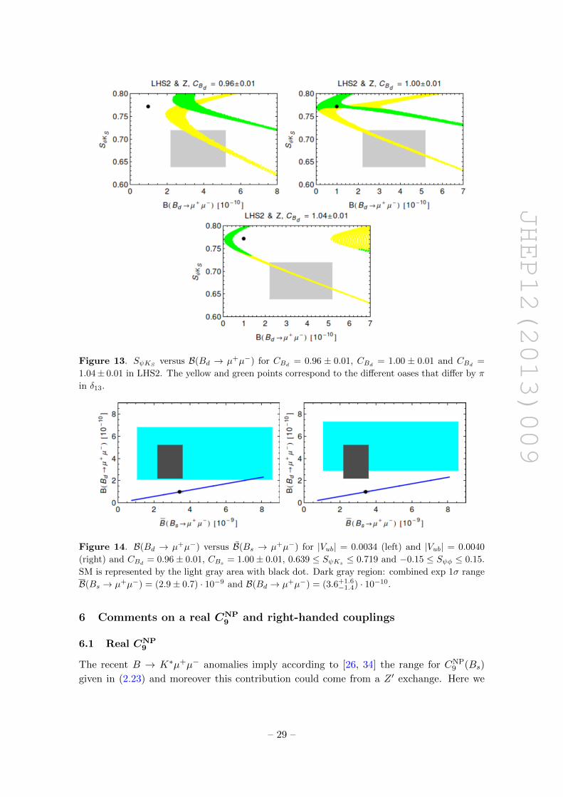
Figure 13. SψKSversus B(Bd → µ+µ−) for CBd

= 0.96 ± 0.01, CBd= 1.00 ± 0.01 and CBd

=

1.04± 0.01 in LHS2. The yellow and green points correspond to the different oases that differ by π

in δ13.

Figure 14. B(Bd → µ+µ−) versus B(Bs → µ+µ−) for |Vub| = 0.0034 (left) and |Vub| = 0.0040

(right) and CBd= 0.96± 0.01, CBs

= 1.00± 0.01, 0.639 ≤ SψKs≤ 0.719 and −0.15 ≤ Sψφ ≤ 0.15.

SM is represented by the light gray area with black dot. Dark gray region: combined exp 1σ range

B(Bs → µ+µ−) = (2.9± 0.7) · 10−9 and B(Bd → µ+µ−) = (3.6+1.6−1.4) · 10−10.

6 Comments on a real CNP9 and right-handed couplings

6.1 Real CNP9

The recent B → K∗µ+µ− anomalies imply according to [26, 34] the range for CNP9 (Bs)

given in (2.23) and moreover this contribution could come from a Z ′ exchange. Here we

– 29 –

JHEP12(2013)009

would like to collect the implications of this possibility for the LHS. These are

• Unique enhancement of ∆Ms with respect to its SM value implying that this scenario

can only be valid for CBs > 1.0. As we have seen in the previous section this is not

favoured by the present data on Bs,d → µ+µ− but cannot be excluded due to large

errors on experimental Bs,d → µ+µ− branching ratios. Future lattice calculations

will tell us whether CBs > 1.0 is true. In fact the most recent values in (4.7) favour

slightly such values.

• As in this case δ23 = βs or δ23 = βs + π, the asymmetry Sψφ equals the SM one. We

are in the scenario for SM-like Sψφ with the restriction CBs > 1.0 and these are the

magenta points in figures 1 and 4. Consequently the CP-asymmetries A7 and A8 in

B → K∗µ+µ− vanish.

• Due to the relation (2.17) there is a strict correlation between B(Bs → µ+µ−) and

CNP9 (Bs) that depends on the values of the ratio ∆µµ

A (Z ′)/∆µµV (Z ′). We show this

correlation in the left panel of figure 15. In the right panel we show using (2.29)

CBs as a function of a real CNP9 (Bs) for different values of ∆µµ

V (Z ′) so that some

correlation between ∆Ms and B(Bs → µ+µ−) is present. The main message from

this plot is that combined data for B(Bs → µ+µ−) and CNP9 favour

0 ≤∆µµA (Z ′)

∆µµV (Z ′)

≤ 1.0, (6.1)

implying that these two couplings should have the same sign.

• While in the Bs system there are some similarities of this scenario with the CMFV

models, LHS differs in the presence of a real CNP9 (Bs) from CMFV as NP physics

with new complex phases can enter Bd and K systems. Moreover as we have seen the

present data on B(Bd → µ+µ−) favour ∆µµA (Z ′) ≈ 1.0 and this can also be correlated

with the results in figure 15.

6.2 Right-handed currents

In [14] we have analyzed in addition to LHS scenario also RHS scenario in which only

right-handed Z ′ couplings where present and two scenarios (LRS and ALRS) with both

left-handed and right-handed couplings satisfying the relations

∆qbL (Z ′) = ∆qb

R (Z ′), ∆qbL (Z ′) = −∆qb

R (Z ′), (6.2)

respectively. Our analysis included complex couplings but in the spirit of this section and

to relate to the analyses in [26, 34] let us assume here that these couplings have the same

phases modulo π so that resulting Wilson coefficients remain real.

To an excellent approximation the shift ∆S in (2.7) is now obtained by making the

following replacement

(∆bsL (Z ′))2 → (∆bs

L (Z ′))2 + (∆bsR (Z ′))2 + κ∆bs

L (Z ′)∆bsR (Z ′), (6.3)

– 30 –

JHEP12(2013)009

Figure 15. B(Bs → µ+µ−) and CBs versus a real CNP9 . Left: ∆µµ

A /∆µµV = −2 (blue dashed), −1

(red dashed), −0.5 (green dashed), 0.5 (green), 1 (red) and 2 (blue). Right: ∆µµV = ±0.5 TeV−1

(blue), ±1 TeV−1 (red) and ±2 TeV−1 (green).

where

κ = 2〈QLR

1 (µZ′)〉〈QVLL

1 (µZ′)〉≈ −10.3 (6.4)

exhibits the known fact that the matrix elements of LR operators are strongly enhanced

with respect to VLL operators that are solely responsible for ∆F = 2 effects in the SM

and LHS scenario. We would like to add that due to different anomalous dimensions of LR

and VLL operators, κ increases with increasing µZ′ = O(MZ′). The value given in (6.4)

corresponds to µZ′ = 1 TeV. For more details, in particular NLO corrections, we refer

to [1, 40]. Analogous expressions for other meson systems exist. Now as seen in table 2

of [1] model independently κ is negative which has an impact on the signs and size of NP

contributions to ∆Ms.

We make the following observations following more detailed discussion in [1, 14]:

• In the case of the RHS scenario the ∆F = 2 constraints are exactly the same as in

the LHS scenario but this time on the right-handed couplings.

• In the case of the LRS scenario with the NP phase aligned to the SM one, NP contri-

bution to ∆Ms is strictly negative as opposed to the LHS scenario and because of the

κ-enhancement the coupling ∆sbL (Z ′) must be suppressed by a factor

√8 relatively

to the LHS or RHS case. For fixed leptonic couplings NP effects in b → sµ+µ−

transitions are expected to be smaller than in LHS scenario. As the contribution is

negative anyway, in the case of establishing CBs > 1.00 this scenario will be ruled

out.

• In the case of ALRS scenario with the NP phase aligned to the SM one, NP con-

tribution to ∆Ms is strictly positive as in the LHS scenario but because of the κ-

enhancement the coupling ∆sbL (Z ′) must be suppressed by a factor

√12 relatively to

the LHS or RHS case. For fixed leptonic couplings NP effects in b→ sµ+µ− transi-

tions are expected to be smaller than in LHS scenario. As the contribution is positive

in the case of establishing CBs < 1.00 this scenario will be ruled out.

– 31 –

JHEP12(2013)009

Concerning Bs,d → µ+µ−, as emphasized in [14], NP effects vanish in the LRS scenario

independently of the leptonic couplings. But it could be that the quark couplings in

Bs → µ+µ− belong to the LRS scenario and this is the reason why the data are close

to the SM prediction, while this is not the case for the quark couplings in Bd → µ+µ−.

In the case of ALRS scenario NP does contribute to Bs,d → µ+µ− and the fact that LH

and RH couplings enter the decay amplitude with the same sign compensates partly the

suppression of quark couplings due to enhanced ∆F = 2 matrix elements.

Let us next investigate Bd → K∗µ+µ− in these scenarios. We concentrate here on

three angular observables FL, S4 and S5 introduced in [74] that are particularly sensitive

to NP contributions. Useful approximate formulae for them in terms of Wilson coefficients

have been recently presented in [26]. These formulae neglect interferences between NP

contributions which is justified in view of small room left for these contributions in the

data. Applied to Z ′ models these formulae are as follows:

〈FL〉[1,6] ≈ 0.77 + 0.05CNP9 − 0.04C ′9 + 0.04C ′10 (6.5)

〈S4〉[14.2,16] ≈ 0.29− 0.02C ′9 + 0.03C ′10. (6.6)

〈S5〉[1,6] ≈ −0.14− 0.09CNP9 − 0.03C ′9 + 0.10C ′10. (6.7)

Here the subscripts on the l.h.s. of these formulae indicate for which bin in q2 these equa-

tions and corresponding data given below apply. In order not to obuse notations we will

drop these subscripts in what follows.

Also in RHS, LRS and ALRS scenarios, NP contributions to the dipole operator can

be neglected [14] and this reduction of the number of relevant Wilson coefficients together

with the absence of new CP-violating phases allows to derive correlations between these

three observables in question as we will see soon. Here the primed coefficients are obtained

from the unprimed ones by replacing ∆qbL (Z ′) by ∆qb

R (Z ′).

It should be emphasized that the numerical values in (6.5)–(6.7) are subject to hadronic

uncertainties. Therefore, even if in our numerical analysis of various correlations we will

use these values, we collect in the appendix A general formulae for these correlations.

This should allow to update these correlations if the numerical values in (6.5)–(6.7) will

be modified. Moreover, from the appendix A one can derive correlations for the basis of

observables proposed in [75] by using the dictionary [26]

S3 =1

2FTP1, S4 =

1

2FLTP

′4, S5 =

1

2FLTP

′5, (6.8)

where FLT =√FL(1− FL).

The first terms in (6.5)–(6.7) are SM predictions. The estimate of uncertainties vary

from paper to paper. We quote here the results from [26]

〈FL〉 = 0.77± 0.04, 〈S4〉 = 0.29± 0.07, 〈S5〉 = −0.14± 0.02. (6.9)

For other estimates see [38, 75]. In particular in [38] much larger error has been assigned

to 〈S5〉.

– 32 –

JHEP12(2013)009

Concerning the data, the ones quoted in [26] and given by

〈FL〉 = 0.59± 0.08, 〈S4〉 = −0.07± 0.11, 〈S5〉 = 0.10± 0.10, (6.10)

are based on the LHCb data for P ′4 and P ′5 [32] and the average of the data from Belle,

Babar, CDF, CMS, ATLAS and LHCb on FL which as discussed in the appendix of [26]

are not in full agreement with each other. We find that the weighted average of the most

accurate data from LHCb [31] and CMS [33] is 〈FL〉 = 0.66 ± 0.07, without basically no

change in S4 and S5. In our plots we will show both ranges on 〈FL〉. Note that the

definition of S4 differs from the LHCb definition by sign.

The central values, in particular for S4 and S5 differ from SM predictions, in particular

the sign of 〈S5〉 is opposite. But the uncertainties both in theory and experiment are sizable.

Still this pattern of deviations could be a sign of NP at work.

Having this formulae at hand it is evident that in LHS, RHS, LRS and ALRS in which

some of the coefficients in question are related to each other correlations between these three

angular observables are present. In the rest of this section we will exhibit these correlations

analytically and graphically neglecting all theoretical uncertainties which certainly are not

small. Our goal is modest: we just want to uncover these correlations as this has not

been done in the literature, leaving a sophisticated numerical analysis for the future when

the data stabilize and a consensus between theorists on the hadronic uncertainties will be

reached. We should also warn the reader that when our results in Z ′ models differ from SM

values by much, the neglect of interferences between different NP contributions cannot be

fully justified but at the semi-quantitative level the presented plots should represent what

is going on.

We can now specify the formulae in (6.5)–(6.6) to the four scenarios in question:

LHS:

〈FL〉 ≈ 0.77 + 0.05CNP9 , (6.11)

〈S4〉 ≈ 0.29, (6.12)

〈S5〉 ≈ −0.14− 0.09CNP9 . (6.13)

Eliminating CNP9 from these expressions in favour of 〈S5〉 we find

〈FL〉 = 0.69− 0.56〈S5〉, (6.14)

which shows analytically the point made in [26, 34] that NP effects in FL and S5 are

anti-correlated as observed in the data.

We show this correlation in the upper left panel in figure 16 together with the data.

We observe that for negative CNP9 = O(1) one can obtain agreement with the data for

these two observables provided such values are also allowed by other constraints. We also

observe that for the larger value of 〈FL〉 (dark grey) it is easier for LHS to describe the

data. On the other hand the value of 〈S4〉 remains SM-like and is significantly larger than

indicated by the data in (6.10). The departure of 〈S4〉 from the SM value would be a sign

of right-handed currents at work. In [26] it has been concluded that it is difficult to find

– 33 –

JHEP12(2013)009

Figure 16. 〈FL〉 versus 〈S5〉 in LHS, RHS, LRS and ALRS. For LHS we have 〈S4〉 = 0 and

the magenta line corresponds to CNP9 = −1.6 ± 0.3 and the cyan line to CNP

9 = −0.8 ± 0.3 as

in (2.23). In the other scenarios (RHS, LRS, ALRS) we choose 〈S4〉 = −0.02 (blue, corresponds to

the experimental central value), 0.1 (red), 0.15 (green), 0.2 (yellow), 0.25 (cyan) and 0.3 (magenta).

The light gray area corresponds to the experimental range in (6.10) and in the dark gray area we

changed 〈FL〉 to 0.66± 0.07 which also slightly change 〈S4,5〉 by a factor 0.963. The light gray line

indicates where the light gray area stops. The black point and the gray box correspond to the SM

predictions from (6.9).

any NP model which could explain the present data on 〈S4〉 and similar conclusion has

been reached in [76]. However, we will keep this observable in our presentation in order to

be prepared for future data.

RHS:

〈FL〉 ≈ 0.77− 0.04C ′9 + 0.04C ′10, (6.15)

〈S4〉 ≈ 0.29− 0.02C ′9 + 0.03C ′10. (6.16)

〈S5〉 ≈ −0.14− 0.03C ′9 + 0.10C ′10. (6.17)

Eliminating C ′10 from these expressions we find

〈FL〉 = 0.826 + 0.40〈S5〉 − 0.028C ′9, (6.18)

〈FL〉 = 0.38 + 1.33〈S4〉 − 0.013C ′9. (6.19)

As seen in figure 17 NP effects in FL and S5 are correlated with each other and this

scenario cannot describe the data even if C ′9 is positive and as large as 2, which is not

– 34 –

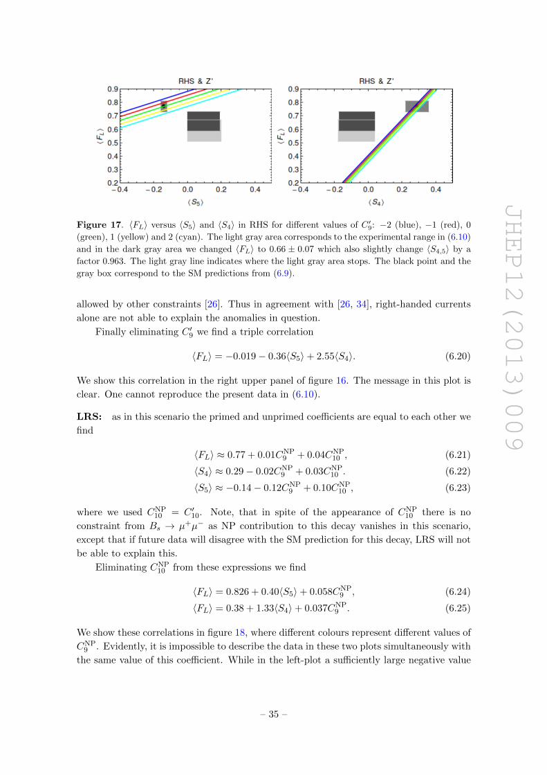
JHEP12(2013)009

Figure 17. 〈FL〉 versus 〈S5〉 and 〈S4〉 in RHS for different values of C ′9: −2 (blue), −1 (red), 0

(green), 1 (yellow) and 2 (cyan). The light gray area corresponds to the experimental range in (6.10)

and in the dark gray area we changed 〈FL〉 to 0.66 ± 0.07 which also slightly change 〈S4,5〉 by a

factor 0.963. The light gray line indicates where the light gray area stops. The black point and the

gray box correspond to the SM predictions from (6.9).

allowed by other constraints [26]. Thus in agreement with [26, 34], right-handed currents

alone are not able to explain the anomalies in question.

Finally eliminating C ′9 we find a triple correlation

〈FL〉 = −0.019− 0.36〈S5〉+ 2.55〈S4〉. (6.20)

We show this correlation in the right upper panel of figure 16. The message in this plot is

clear. One cannot reproduce the present data in (6.10).

LRS: as in this scenario the primed and unprimed coefficients are equal to each other we

find

〈FL〉 ≈ 0.77 + 0.01CNP9 + 0.04CNP

10 , (6.21)

〈S4〉 ≈ 0.29− 0.02CNP9 + 0.03CNP

10 . (6.22)

〈S5〉 ≈ −0.14− 0.12CNP9 + 0.10CNP

10 , (6.23)

where we used CNP10 = C ′10. Note, that in spite of the appearance of CNP

10 there is no

constraint from Bs → µ+µ− as NP contribution to this decay vanishes in this scenario,

except that if future data will disagree with the SM prediction for this decay, LRS will not

be able to explain this.

Eliminating CNP10 from these expressions we find

〈FL〉 = 0.826 + 0.40〈S5〉+ 0.058CNP9 , (6.24)

〈FL〉 = 0.38 + 1.33〈S4〉+ 0.037CNP9 . (6.25)

We show these correlations in figure 18, where different colours represent different values of

CNP9 . Evidently, it is impossible to describe the data in these two plots simultaneously with

the same value of this coefficient. While in the left-plot a sufficiently large negative value

– 35 –

JHEP12(2013)009

Figure 18. 〈FL〉 versus 〈S5〉 and 〈S4〉 in LRS for different values of CNP9 : −2 (blue), −1 (red), 0

(green) and 1 (yellow). The light gray area corresponds to the experimental range in (6.10) and

in the dark gray area we changed 〈FL〉 to 0.66± 0.07 which also slightly change 〈S4,5〉 by a factor

0.963. The light gray line indicates where the light gray area stops. The black point and the gray

box correspond to the SM predictions from (6.9).

of CNP9 would help in explaining the data, in the right plot a positive value is required.

This is also seen in figure 16 where we show the triple correlation which one obtains after

eliminating CNP9

〈FL〉 = −0.38− 0.688〈S5〉+ 3.63〈S4〉. (6.26)

ALRS: as in this scenario the primed and unprimed coefficients differ by sign we find

〈FL〉 ≈ 0.77 + 0.09CNP9 − 0.04CNP

10 , (6.27)

〈S4〉 ≈ 0.29 + 0.02CNP9 − 0.03CNP

10 , (6.28)

〈S5〉 ≈ −0.14− 0.06CNP9 − 0.10CNP

10 , (6.29)

where we used CNP10 = −C ′10. We find in this case the following correlations

〈FL〉 = 0.826 + 0.40〈S5〉+ 0.114CNP9 , (6.30)

〈FL〉 = 0.38 + 1.33〈S4〉+ 0.063CNP9 . (6.31)

In fact this scenario is rather close to the one investigated numerically in [26]. We show

these correlations in figure 19. The one between 〈FL〉 and 〈S4〉 is basically unchanged

relatively to the LRS case while the one between 〈FL〉 and 〈S5〉 appears to be in a better

shape when compared with the data. In fact as emphasized in [26] it is easier to obtain

the agreement with the data on 〈FL〉 and 〈S5〉 by including a non-vanishing C ′9 in addition

to CNP9 . As seen in the left plot of figure 4 in the latter paper, the data on AFB and

B → Kµ+µ− favour C ′9 to be of similar magnitude as CNP9 but having opposite sign and

this is our ALRS scenario.

Finally, we find the triple correlation

〈FL〉 = −0.17− 0.50〈S5〉+ 3.00〈S4〉, (6.32)

– 36 –

JHEP12(2013)009

Figure 19. 〈FL〉 versus 〈S5〉 and 〈S4〉 in ALRS for different values of CNP9 : −2 (blue), −1 (red),

0 (green) and 1 (yellow). The light gray area corresponds to the experimental range in (6.10) and

in the dark gray area we changed 〈FL〉 to 0.66± 0.07. The light gray line indicates where the light

gray area stops. The black point and the gray box correspond to the SM predictions from (6.9).

which we show in the lower right panel in figure 16. Again we observe the problem with

describing the data on 〈S4〉.Clearly a complete analysis must include constraints on the values of CNP

9 from other

observables but such an analysis in the scenarios with right-handed currents is beyond the

scope of the present paper. We refer to [26] for a sophisticated model independent numerical

analysis of such scenarios which also involve the coefficients of the dipole operators which

in Z ′ models are very suppressed.

The summary of this short excursion in the world of right-handed currents is as follows:

• The finalists in the competition between these four scenarios are LHS and ALRS and

in agreement with [26] the present data on 〈FL〉 and 〈S5〉 seem to favour ALRS over

LHS.

• In order for these finalists to work the future experimental value of 〈S4〉 must be

SM-like. This is in particular the case of LHS scenario. In ALRS this implies as seen

in (6.6)

CNP10 ≈

2

3CNP

9 (6.33)

and the correlation with Bs → µ+µ− decay. We find then that B(Bs → µ+µ−) ≥4.6 · 10−9.

In order to understand this result let us recall that with real NP contributions to

the Wilson coefficients a positive (negative) C ′10 enhances (suppresses) the Bs → µ+µ−

branching ratio while the opposite is true for CNP10 . In the ALRS scenario C ′10 = −CNP

10

and taking into account that the data on 〈FL〉 and 〈S5〉 require a negative CNP9 implies

through (6.33) an enhancement of B(Bs → µ+µ−), which could be problematic for ALRS

one day.

No such correlation is present in LHS but in this scenario as shown at the beginning of

this section, a real CNP9 implies uniquely an enhancement of ∆Ms and CBs > 1.00, which

– 37 –

JHEP12(2013)009

Figure 20. B(Bd → Kµ+µ−) versus B(Bs → µ+µ−) in LHS for different values of CNP9 : −2 (blue),

−1 (red), 0 (green), 1 (yellow) and 2 (cyan) and −0.8 ≤ CNP10 ≤ 1.8. The gray area corresponds to

the experimental range in (6.35). SM is represented by the black point.

is not favoured by our analysis of Bs,d → µ+µ−. Solution to this possible problem are new

CP-violating phases and this could be tested in Bd → K∗µ+µ− by the measurements of

the CP-asymmetries A7 and A8.

Finally let us emphasize that the decay Bd → Kµ+µ− can also contribute to this

discussion. Indeed the authors of [26] provided an approximate formula for the branching

ratio confined to large q2 region. Lattice calculations of the relevant form factors are making

significant progress here [77, 78] and the importance of this decay will increase in the future.

For real Wilson coefficients and neglecting the interference between NP contributions the

formula of [26] reduces in the absence of NP contributions to Wilson coefficients of dipole

operators to

107 × B(Bd → Kµ+µ−)[14.2,22] = 1.11 + 0.27 (CNP9 + C ′9)− 0.27 (CNP

10 + C ′10) (6.34)

where the error on the first SM term is estimated to be 10% [77, 78]. This should be

compared with the LHCb result

107 × B(Bd → Kµ+µ−)[14.2,22] = 1.04± 0.12 (LHCb). (6.35)

We can now explicitly see what happens in the four scenarios discussed by us.

• For LHS we find

107 × B(Bd → Kµ+µ−)[14.2,22] = 1.11 + 0.27 (CNP9 − CNP

10 ), (6.36)

while for RHS the Wilson coefficients CNP9,10 should be replaced by C ′9,10. As RHS is

not a favourite scenario we will not consider it further.

• For LRS we simply have

107 × B(Bd → Kµ+µ−)[14.2,22] = 1.11 + 0.54 (CNP9 − CNP

10 ). (6.37)

In this scenario NP contributions to Bs → µ+µ− vanish but as seen in this formula

they could still be visible in Bd → Kµ+µ− and this is a characteristic feature of this

scenario.

– 38 –

JHEP12(2013)009

• The opposite takes place in ALRS where NP contributions to Bs → µ+µ− can be

present but vanish for Bd → Kµ+µ−. In this scenario there is no constraint on

angular observables from Bd → Kµ+µ−.

As stressed in [26] the Wilson coefficient CNP9 by itself has difficulty in removing com-

pletely the anomalies in Bd → K∗µ+µ− due to the constraint from Bd → Kµ+µ−. The

LHS scenario allows us to have a closer look at this issue. Using (6.36) we show in figure 20

the correlation between B(Bd → Kµ+µ−)[14.2,22] and B(Bs → µ+µ−) for various values

of CNP9 . We show also the ±10% error on SM prediction which should also be taken into

account in the lines corresponding to NP predictions with CNP9 6= 0. Indeed in agreement

with [26] only |CNP9 | ≤ 1.0 is allowed at 1σ which is insufficient, as seen in figure 16, to

remove completely Bd → K∗µ+µ− anomalies.

7 Conclusions and outlook

Motivated by recent experimental results on Bs,d → µ+µ− and B → K∗µ+µ− we have

revisited the LHS scenario of [14] generalizing it to arbitrary MZ′ , ∆µµA (Z ′) and departures

of (∆Ms,d)SM from the data. This allowed us to present new correlations between various

observables. These correlations, shown in many figures will allow in the coming years

to monitor whether LHS can describe future more precise data when also lattice results

improve. As already emphasized at the beginning of our paper this will certainly be non-

trivial.

Beyond these correlations possibly the most important results of this paper are the

following ones:

• LHS provides a simple model that allows for the violation of the CMFV relation

between the branching ratios for Bd,s → µ+µ− and ∆Ms,d. The plots in figures 9

and 14 for Z ′ and Z illustrate this.

• Moreover, LHS is able to accommodate the recent experimental results for Bs,d →µ+µ− but this in the case of B(Bd → µ+µ−) requires ∆µµ

A (Z ′) ≥ 1.0 and larger by a

factor of two relative to the one considered by us in [14].

• The SM Z boson with FCNC couplings to quarks can describe the present data on

Bs,d → µ+µ− provided ∆Ms and Sψφ are very close to their SM values. However,

in view of its small vector coupling to muons it cannot describe the anomalies in

Bd → K∗µ+µ−.

• The explanation of the present anomalies in Bd → K∗µ+µ− with a real CNP9 (Bs) as

proposed in [26, 34] implies uniquely an enhancement of ∆Ms over its SM value. As

the present SM value for the ratio ∆Ms/∆Md agrees with the data very well, it is

likely that also ∆Md should be enhanced in this scenario to agree with experiment.

For this pattern to agree with the data the values of the non-perturbative parameters

in ∆Ms,d have to be lower than their present central values.

– 39 –

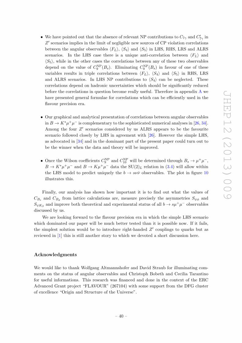
JHEP12(2013)009

• We have pointed out that the absence of relevant NP contributions to C7γ and C ′7γ in

Z ′ scenarios implies in the limit of negligible new sources of CP violation correlations

between the angular observables 〈FL〉, 〈S4〉 and 〈S5〉 in LHS, RHS, LRS and ALRS

scenarios. In the LHS case there is a unique anti-correlation between 〈FL〉 and

〈S5〉, while in the other cases the correlations between any of these two observables

depend on the value of CNP9 (Bs). Eliminating CNP

9 (Bs) in favour of one of these

variables results in triple correlations between 〈FL〉, 〈S4〉 and 〈S5〉 in RHS, LRS

and ALRS scenarios. In LHS NP contributions to 〈S4〉 can be neglected. These

correlations depend on hadronic uncertainties which should be significantly reduced

before the correlations in question become really useful. Therefore in appendix A we

have presented general formulae for correlations which can be efficiently used in the

flavour precision era.

• Our graphical and analytical presentation of correlations between angular observables

in B → K∗µ+µ− is complementary to the sophisticated numerical analyses in [26, 34].

Among the four Z ′ scenarios considered by us ALRS appears to be the favourite

scenario followed closely by LHS in agreement with [26]. However the simple LHS,

as advocated in [34] and in the dominant part of the present paper could turn out to

be the winner when the data and theory will be improved.

• Once the Wilson coefficients CNP9 and CNP

10 will be determined through Bs → µ+µ−,

B → K∗µ+µ− and B → Kµ+µ− data the SU(2)L relation in (3.4) will allow within

the LHS model to predict uniquely the b → sνν observables. The plot in figure 10

illustrates this.

Finally, our analysis has shown how important it is to find out what the values of

CBs and CBdfrom lattice calculations are, measure precisely the asymmetries Sψφ and

SψKSand improve both theoretical and experimental status of all b→ sµ+µ− observables

discussed by us.

We are looking forward to the flavour precision era in which the simple LHS scenario

which dominated our paper will be much better tested than it is possible now. If it fails,

the simplest solution would be to introduce right-handed Z ′ couplings to quarks but as

reviewed in [1] this is still another story to which we devoted a short discussion here.

Acknowledgments

We would like to thank Wolfgang Altmannshofer and David Straub for illuminating com-

ments on the status of angular observables and Christoph Bobeth and Cecilia Tarantino

for useful informations. This research was financed and done in the context of the ERC

Advanced Grant project “FLAVOUR” (267104) with some support from the DFG cluster

of excellence “Origin and Structure of the Universe”.

– 40 –

JHEP12(2013)009

A General formulae for correlations

In the limit of no new CP-violating phases and neglecting the contributions of dipole

operators as well as interferences between NP contributions one can generally write

〈∆FL〉 ≡ 〈FL〉 − 〈FL〉SM = a9CNP9 + a9′C

′9 + a10′C

′10, (A.1)

〈∆S4〉 ≡ 〈S4〉 − 〈S4〉SM = b9′C′9 + b10′C

′10, (A.2)

〈∆S5〉 ≡ 〈S5〉 − 〈S5〉SM = d9CNP9 + d9′C

′9 + d10′C

′10 . (A.3)

The coefficients ai, bi and di are subject to hadronic uncertainties. For the form factors

used in [26] one has (6.5)–(6.7) but as these coefficients will change with time it is useful

to present general expressions. In particular one can derive correlations between 〈∆FL〉,〈∆S4〉 and 〈∆S5〉.

In the LHS scenario we simply have

〈∆FL〉 =a9

d9〈∆S5〉, 〈∆S4〉 = 0 . (A.4)

For LR and ALRS scenarios we introduce

r±1 = a9 ± a9′ −a10′

d10′(d9 ± d9′) (A.5)

r±2 = a9 ± a9′ ∓a10′

b10′b9′ (A.6)

with r+1,2 for LRS and r−1,2 for ALRS.

Then we find the correlations

〈∆FL〉 =a10′

d10′〈∆S5〉+ r±1 C

NP9 (A.7)

〈∆FL〉 =a10′

b10′〈∆S4〉+ r±2 C

NP9 (A.8)

and the triple correlation(1− r±1

r±2

)〈∆FL〉 =

a10′

d10′〈∆S5〉 −

r±1r±2

a10′

b10′〈∆S4〉. (A.9)

In the RHS scenario one should set a9 = d9 = 0 and CNP9 = C ′9 in this formulae and

use r+1,2.

Inserting the numerical values for ai, bi and di given in (6.5)–(6.7) into these formulae

one recovers the correlations used in our numerical analysis.

References

[1] A.J. Buras and J. Girrbach, Towards the Identification of New Physics through Quark

Flavour Violating Processes, arXiv:1306.3775 [INSPIRE].

[2] A. Buras, P. Gambino, M. Gorbahn, S. Jager and L. Silvestrini, Universal unitarity triangle

and physics beyond the standard model, Phys. Lett. B 500 (2001) 161 [hep-ph/0007085]

[INSPIRE].

– 41 –

JHEP12(2013)009

[3] A.J. Buras, Minimal flavor violation, Acta Phys. Polon. B 34 (2003) 5615 [hep-ph/0310208]

[INSPIRE].

[4] R.S. Chivukula and H. Georgi, Composite Technicolor Standard Model, Phys. Lett. B 188

(1987) 99 [INSPIRE].

[5] L. Hall and L. Randall, Weak scale effective supersymmetry, Phys. Rev. Lett. 65 (1990) 2939

[INSPIRE].

[6] G. D’Ambrosio, G. Giudice, G. Isidori and A. Strumia, Minimal flavor violation: an

Effective field theory approach, Nucl. Phys. B 645 (2002) 155 [hep-ph/0207036] [INSPIRE].

[7] A.L. Kagan, G. Perez, T. Volansky and J. Zupan, General Minimal Flavor Violation, Phys.

Rev. D 80 (2009) 076002 [arXiv:0903.1794] [INSPIRE].

[8] R. Barbieri, G. Isidori, J. Jones-Perez, P. Lodone and D.M. Straub, U(2) and Minimal

Flavour Violation in Supersymmetry, Eur. Phys. J. C 71 (2011) 1725 [arXiv:1105.2296]

[INSPIRE].

[9] R. Barbieri, D. Buttazzo, F. Sala and D.M. Straub, Flavour physics from an approximate

U(2)3 symmetry, JHEP 07 (2012) 181 [arXiv:1203.4218] [INSPIRE].

[10] A. Crivellin, L. Hofer and U. Nierste, The MSSM with a Softly Broken U(2)3 Flavor

Symmetry, PoS(EPS-HEP2011)145, [arXiv:1111.0246] [INSPIRE].

[11] A.J. Buras and J. Girrbach, On the Correlations between Flavour Observables in Minimal

U(2)3 Models, JHEP 01 (2013) 007 [arXiv:1206.3878] [INSPIRE].

[12] W. Altmannshofer, A.J. Buras, S. Gori, P. Paradisi and D.M. Straub, Anatomy and

Phenomenology of FCNC and CPV Effects in SUSY Theories, Nucl. Phys. B 830 (2010) 17

[arXiv:0909.1333] [INSPIRE].

[13] A.J. Buras, F. De Fazio, J. Girrbach and M.V. Carlucci, The Anatomy of Quark Flavour

Observables in 331 Models in the Flavour Precision Era, JHEP 02 (2013) 023

[arXiv:1211.1237] [INSPIRE].

[14] A.J. Buras, F. De Fazio and J. Girrbach, The Anatomy of Z’ and Z with Flavour Changing

Neutral Currents in the Flavour Precision Era, JHEP 02 (2013) 116 [arXiv:1211.1896]

[INSPIRE].

[15] A.J. Buras, J. Girrbach and R. Ziegler, Particle-Antiparticle Mixing, CP-violation and Rare

K and B Decays in a Minimal Theory of Fermion Masses, JHEP 04 (2013) 168

[arXiv:1301.5498] [INSPIRE].

[16] A.J. Buras, R. Fleischer, J. Girrbach and R. Knegjens, Probing New Physics with the

Bs → µ+µ− Time-Dependent Rate, JHEP 1307 (2013) 77 [arXiv:1303.3820] [INSPIRE].

[17] A.J. Buras, F. De Fazio, J. Girrbach, R. Knegjens and M. Nagai, The Anatomy of Neutral

Scalars with FCNCs in the Flavour Precision Era, JHEP 06 (2013) 111 [arXiv:1303.3723]

[INSPIRE].

[18] P. Langacker, The Physics of Heavy Z ′ Gauge Bosons, Rev. Mod. Phys. 81 (2009) 1199

[arXiv:0801.1345] [INSPIRE].

[19] V. Barger et al., b→ s Transitions in Family-dependent U(1)′ Models, JHEP 12 (2009) 048

[arXiv:0906.3745] [INSPIRE].

[20] P.J. Fox, J. Liu, D. Tucker-Smith and N. Weiner, An Effective Z’, Phys. Rev. D 84 (2011)

115006 [arXiv:1104.4127] [INSPIRE].

[21] W. Altmannshofer, P. Paradisi and D.M. Straub, Model-Independent Constraints on New

Physics in b→ s Transitions, JHEP 04 (2012) 008 [arXiv:1111.1257] [INSPIRE].

– 42 –

JHEP12(2013)009

[22] W. Altmannshofer and D.M. Straub, Cornering New Physics in b→ s Transitions, JHEP 08

(2012) 121 [arXiv:1206.0273] [INSPIRE].

[23] A. Dighe and D. Ghosh, How large can the branching ratio of Bs → τ+τ− be?, Phys. Rev. D

86 (2012) 054023 [arXiv:1207.1324] [INSPIRE].

[24] S. Sun, D.B. Kaplan and A.E. Nelson, Little flavor: a model of weak-scale flavor physics,

Phys. Rev. D 87 (2013) 125036 [arXiv:1303.1811] [INSPIRE].

[25] A.J. Buras, Relations between ∆Ms,d and Bs,d → µ+µ− in models with minimal flavor

violation, Phys. Lett. B 566 (2003) 115 [hep-ph/0303060] [INSPIRE].

[26] W. Altmannshofer and D.M. Straub, New physics in B → K∗µµ?, arXiv:1308.1501

[INSPIRE].

[27] R. Gauld, F. Goertz and U. Haisch, On minimal Z’ explanations of the B → K∗µ+µ−

anomaly, arXiv:1308.1959 [INSPIRE].

[28] LHCb collaboration, Measurement of the B0s → µ+µ− branching fraction and search for

B0 → µ+µ− decays at the LHCb experiment, Phys. Rev. Lett. 111 (2013) 101805

[arXiv:1307.5024] [INSPIRE].

[29] CMS collaboration, Measurement of the Bs → µµ branching fraction and search for B0 → µµ

with the CMS Experiment, Phys. Rev. Lett. 111 (2013) 101804 [arXiv:1307.5025] [INSPIRE].

[30] CMS and LHCb collaborations, Combination of results on the rare decays B0(s) → µ+µ− from

the CMS and LHCb experiments, CMS-PAS-BPH-13-007 (2013).

[31] LHCb collaboration, Differential branching fraction and angular analysis of the decay

B0 → K∗0µ+µ−, JHEP 08 (2013) 131 [arXiv:1304.6325] [INSPIRE].

[32] LHCb collaboration, Measurement of form-factor independent observables in the decay

B0 → K∗0µ+µ−, Phys. Rev. Lett. 111 (2013) 191801 [arXiv:1308.1707] [INSPIRE].

[33] CMS collaboration, Angular analysis and branching fraction measurement of the decay

B0 → K∗0µ+µ−, Phys. Lett. B 727 (2013) 77 [arXiv:1308.3409] [INSPIRE].

[34] S. Descotes-Genon, J. Matias and J. Virto, Understanding the B → K∗µ+µ− Anomaly,

Phys. Rev. D 88 (2013) 074002 [arXiv:1307.5683] [INSPIRE].

[35] A. Khodjamirian, T. Mannel, A. Pivovarov and Y.-M. Wang, Charm-loop effect in

B → K(∗)`+`− and B → K∗γ, JHEP 09 (2010) 089 [arXiv:1006.4945] [INSPIRE].

[36] M. Beylich, G. Buchalla and T. Feldmann, Theory of B → K(∗)`+`− decays at high q2: OPE

and quark-hadron duality, Eur. Phys. J. C 71 (2011) 1635 [arXiv:1101.5118] [INSPIRE].

[37] J. Matias, On the S-wave pollution of B → K∗`+`− observables, Phys. Rev. D 86 (2012)

094024 [arXiv:1209.1525] [INSPIRE].

[38] S. Jager and J. Martin Camalich, On B → V `` at small dilepton invariant mass, power

corrections and new physics, JHEP 05 (2013) 043 [arXiv:1212.2263] [INSPIRE].

[39] D. Guadagnoli and G. Isidori, BR(Bs → µ+µ−) as an electroweak precision test,

arXiv:1302.3909 [INSPIRE].

[40] A.J. Buras and J. Girrbach, Complete NLO QCD Corrections for Tree Level Delta F = 2

FCNC Processes, JHEP 03 (2012) 052 [arXiv:1201.1302] [INSPIRE].

[41] A.J. Buras, M. Jamin and P.H. Weisz, Leading and Next-to-leading QCD Corrections to ε

Parameter and B0 − B0 Mixing in the Presence of a Heavy Top Quark, Nucl. Phys. B 347

(1990) 491 [INSPIRE].

– 43 –

JHEP12(2013)009

[42] C. Bobeth, P. Gambino, M. Gorbahn and U. Haisch, Complete NNLO QCD analysis of

B → Xs`+`− and higher order electroweak effects, JHEP 04 (2004) 071 [hep-ph/0312090]

[INSPIRE].

[43] T. Huber, E. Lunghi, M. Misiak and D. Wyler, Electromagnetic logarithms in B → Xs`+`−,

Nucl. Phys. B 740 (2006) 105 [hep-ph/0512066] [INSPIRE].

[44] A.J. Buras and M. Munz, Effective Hamiltonian for B → Xse+e− beyond leading logarithms

in the NDR and HV schemes, Phys. Rev. D 52 (1995) 186 [hep-ph/9501281] [INSPIRE].

[45] C. Bobeth, M. Misiak and J. Urban, Photonic penguins at two loops and mt dependence of

BR(B → Xs`+`−), Nucl. Phys. B 574 (2000) 291 [hep-ph/9910220] [INSPIRE].

[46] C. Bobeth, M. Misiak and J. Urban, Matching conditions for b→ sγ and b→ s gluon in

extensions of the standard model, Nucl. Phys. B 567 (2000) 153 [hep-ph/9904413] [INSPIRE].

[47] A.J. Buras, L. Merlo and E. Stamou, The Impact of Flavour Changing Neutral Gauge

Bosons on B → Xsγ, JHEP 08 (2011) 124 [arXiv:1105.5146] [INSPIRE].

[48] K. De Bruyn, R. Fleischer, R. Knegjens, P. Koppenburg, M. Merk et al., Probing New

Physics via the B0s → µ+µ− Effective Lifetime, Phys. Rev. Lett. 109 (2012) 041801

[arXiv:1204.1737] [INSPIRE].

[49] R. Fleischer, On Branching Ratios of Bs Decays and the Search for New Physics in

B0s → µ+µ−, Nucl. Phys. Proc. Suppl. 241-242 (2013) 135 [arXiv:1208.2843] [INSPIRE].

[50] A.J. Buras, J. Girrbach, D. Guadagnoli and G. Isidori, On the Standard Model prediction for

BR(Bs,d → µ+µ−), Eur. Phys. J. C 72 (2012) 2172 [arXiv:1208.0934] [INSPIRE].

[51] F. Beaujean, C. Bobeth, D. van Dyk and C. Wacker, Bayesian Fit of Exclusive b→ s ¯

Decays: the Standard Model Operator Basis, JHEP 08 (2012) 030 [arXiv:1205.1838]

[INSPIRE].

[52] C. Bobeth, G. Hiller and D. van Dyk, General Analysis of B → K(∗)`+`− Decays at Low

Recoil, Phys. Rev. D 87 (2013) 034016 [arXiv:1212.2321] [INSPIRE].

[53] F. Beaujean, C. Bobeth and D. van Dyk, Comprehensive Bayesian Analysis of Rare

(Semi)leptonic and Radiative B Decays, arXiv:1310.2478 [INSPIRE].

[54] R.R. Horgan, Z. Liu, S. Meinel and M. Wingate, Calculation of B0 → K∗0µ+µ− and

B0s → φµ+µ− observables using form factors from lattice QCD, arXiv:1310.3887 [INSPIRE].

[55] G. Colangelo et al., Review of lattice results concerning low energy particle physics, Eur.

Phys. J. C 71 (2011) 1695 [arXiv:1011.4408] [INSPIRE].

[56] T. Hurth, G. Isidori, J.F. Kamenik and F. Mescia, Constraints on New Physics in MFV

models: a Model-independent analysis of ∆F = 1 processes, Nucl. Phys. B 808 (2009) 326

[arXiv:0807.5039] [INSPIRE].

[57] N. Carrasco et al., B-physics from Nf=2 tmQCD: the Standard Model and beyond,

arXiv:1308.1851 [INSPIRE].

[58] J. Laiho, E. Lunghi and R.S. Van de Water, Lattice QCD inputs to the CKM unitarity

triangle analysis, Phys. Rev. D 81 (2010) 034503 [arXiv:0910.2928] [INSPIRE].

[59] A.J. Buras and J. Girrbach, Stringent Tests of Constrained Minimal Flavour Violation

through ∆F = 2 Transitions, The European Physical Journal C 9 (73) 2013

[arXiv:1304.6835] [INSPIRE].

[60] W. Marciano and A. Sirlin, Constraint on Additional Neutral Gauge Bosons From

Electroweak Radiative Corrections, Phys. Rev. D 35 (1987) 1672 [INSPIRE].

– 44 –

JHEP12(2013)009

[61] W. Altmannshofer, A.J. Buras, D.M. Straub and M. Wick, New strategies for New Physics

search in B → K∗νν, B → Kνν and B → Xsνν decays, JHEP 04 (2009) 022

[arXiv:0902.0160] [INSPIRE].

[62] Heavy Flavor Averaging Group collaboration, Y. Amhis et al., Averages of B-Hadron,

C-Hadron and tau-lepton properties as of early 2012, arXiv:1207.1158 [INSPIRE].

[63] LHCb collaboration, Measurement of CP violation and the B0s meson decay width difference

with B0s → J/ψK+K− and B0

s → J/ψπ+π− decays, Phys. Rev. D 87 (2013) 112010

[arXiv:1304.2600] [INSPIRE].

[64] UTfit collaboration, M. Bona et al., Constraints on new physics from the quark mixing

unitarity triangle, Phys. Rev. Lett. 97 (2006) 151803 [hep-ph/0605213] [INSPIRE].

[65] D.M. Straub, Constraints on new physics from rare (semi-)leptonic B decays,

arXiv:1305.5704 [INSPIRE].

[66] W. Altmannshofer, The Bs → µ+µ− and Bd → µ+µ− Decays: Standard Model and Beyond,

PoS(Beauty 2013)024 [arXiv:1306.0022] [INSPIRE].

[67] P. Colangelo, F. De Fazio, P. Santorelli and E. Scrimieri, Rare B → K(∗) neutrino

anti-neutrino decays at B factories, Phys. Lett. B 395 (1997) 339 [hep-ph/9610297]

[INSPIRE].

[68] G. Buchalla, G. Hiller and G. Isidori, Phenomenology of nonstandard Z couplings in exclusive

semileptonic b→ s transitions, Phys. Rev. D 63 (2000) 014015 [hep-ph/0006136] [INSPIRE].

[69] M. Blanke, A.J. Buras, B. Duling, S. Recksiegel and C. Tarantino, FCNC Processes in the

Littlest Higgs Model with T-Parity: a 2009 Look, Acta Phys. Polon. B 41 (2010) 657

[arXiv:0906.5454] [INSPIRE].

[70] O. Eberhardt et al., Impact of a Higgs boson at a mass of 126 GeV on the standard model

with three and four fermion generations, Phys. Rev. Lett. 109 (2012) 241802

[arXiv:1209.1101] [INSPIRE].

[71] A.J. Buras et al., Patterns of Flavour Violation in the Presence of a Fourth Generation of

Quarks and Leptons, JHEP 09 (2010) 106 [arXiv:1002.2126] [INSPIRE].

[72] G.W.S. Hou, Enhanced Bd → µ+µ− Decay: what if?, arXiv:1307.2448 [INSPIRE].

[73] M. Blanke, A.J. Buras, B. Duling, K. Gemmler and S. Gori, Rare K and B Decays in a

Warped Extra Dimension with Custodial Protection, JHEP 03 (2009) 108

[arXiv:0812.3803] [INSPIRE].

[74] W. Altmannshofer et al., Symmetries and Asymmetries of B → K∗µ+µ− Decays in the

Standard Model and Beyond, JHEP 01 (2009) 019 [arXiv:0811.1214] [INSPIRE].

[75] S. Descotes-Genon, T. Hurth, J. Matias and J. Virto, Optimizing the basis of B → K∗`+`−

observables in the full kinematic range, JHEP 05 (2013) 137 [arXiv:1303.5794] [INSPIRE].

[76] C. Hambrock, G. Hiller, S. Schacht and R. Zwicky, B → K∗ Form Factors from Flavor Data

to QCD and Back, arXiv:1308.4379 [INSPIRE].

[77] C. Bouchard, G.P. Lepage, C. Monahan, H. Na and J. Shigemitsu, Standard Model

predictions for B → Kll with form factors from lattice QCD, Phys. Rev. Lett. 111 (2013)

162002 [arXiv:1306.0434] [INSPIRE].

[78] C. Bouchard, G.P. Lepage, C. Monahan, H. Na and J. Shigemitsu, Rare decay B → Kll form

factors from lattice QCD, Phys. Rev. D 88 (2013) 054509 [arXiv:1306.2384] [INSPIRE].

– 45 –