Lecture 7 Asymptotics of OLS - Bauer College of Business · -A sufficient condition for consistency...
47
RS – Lecture 7 1 1 Lecture 7 Asymptotics of OLS OLS Estimation - Assumptions • CLM Assumptions (A1) DGP: y = X + is correctly specified. (A2) E[|X] = 0 (A3) Var[|X] = σ 2 I T (A4) X has full column rank – rank(X)=k-, where T ≥ k. • From (A1), (A2), and (A4) b = (X′X) -1 X′ y • Using (A3) Var[b|X] = σ 2 (XX) -1 • Adding (A5) |X ~iid N(0, σ 2 I T ) b|X ~iid N(, σ 2 (XX) -1 ) (A5) gives us finite sample results for b (& for the t-test, F-test, Wald test) • In this lecture, we will relax (A5). We will focus on the behavior of b (and the test statistics) when T → ∞ –i.e., large samples.
Transcript of Lecture 7 Asymptotics of OLS - Bauer College of Business · -A sufficient condition for consistency...
RS – Lecture 7
1
1
Lecture 7Asymptotics of OLS
OLS Estimation - Assumptions
• CLM Assumptions
(A1) DGP: y = X + is correctly specified.
(A2) E[|X] = 0
(A3) Var[|X] = σ2 IT
(A4) X has full column rank – rank(X)=k-, where T ≥ k.
• From (A1), (A2), and (A4) b = (X′X)-1X′ y
• Using (A3) Var[b|X] = σ2(XX)-1
• Adding (A5) |X ~iid N(0, σ2IT) b|X ~iid N(, σ2(XX)-1)
(A5) gives us finite sample results for b (& for the t-test, F-test, Wald test)
• In this lecture, we will relax (A5). We will focus on the behavior of b (and the test statistics) when T → ∞ –i.e., large samples.
RS – Lecture 7
2
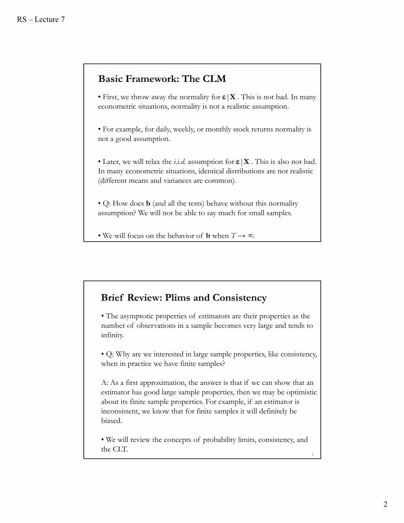
• First, we throw away the normality for |X . This is not bad. In many econometric situations, normality is not a realistic assumption.
• For example, for daily, weekly, or monthly stock returns normality is not a good assumption.
• Later, we will relax the i.i.d. assumption for |X . This is also not bad. In many econometric situations, identical distributions are not realistic (different means and variances are common).
• Q: How does b (and all the tests) behave without this normality assumption? We will not be able to say much for small samples.
• We will focus on the behavior of b when T → ∞.
Basic Framework: The CLM
2
• The asymptotic properties of estimators are their properties as the number of observations in a sample becomes very large and tends to infinity.
• Q: Why are we interested in large sample properties, like consistency, when in practice we have finite samples?
A: As a first approximation, the answer is that if we can show that an estimator has good large sample properties, then we may be optimistic about its finite sample properties. For example, if an estimator is inconsistent, we know that for finite samples it will definitely be biased.
• We will review the concepts of probability limits, consistency, and the CLT.
Brief Review: Plims and Consistency
RS – Lecture 7
3
Probability Limit: Convergence in probability
• Definition: Convergence in probability Let θ be a constant, ε > 0, and n be the index of the sequence of RV xn. If limn→∞ Prob[|xn – θ|> ε ] = 0 for any ε > 0, we say that xnconverges in probability to θ.
That is, the probability that the difference between xn and θ is larger than any ε>0 goes to zero as n becomes bigger.
Notation: xn θplim xn = θ
• If xn is an estimator (for example, the sample mean) and if plim xn =θ, we say that xn is a consistent estimator of θ.
Estimators can be inconsistent. For example, when they are consistent for something other than our parameter of interest.
p
• Theorem: Convergence for sample moments.
Under certain assumptions (for example, i.i.d. with finite mean), sample moments converge in probability to their population counterparts.
We saw this theorem before. It’s the (Weak) Law of Large Numbers (LLN). Different assumptions create different versions of the LLN.
Note: The LLN is very general:
(1/n)Σif (zi) E[f (zi)].
• The usual version in Greene assumes i.i.d. with finite mean. This is the Khinchin’s (1929) (weak) LLN. (Khinchin is also spelled Khintchine)
p
Probability Limit: Weak Law of Large Numbers
RS – Lecture 7
4
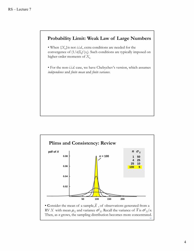
• When {Xn}is not i.i.d., extra conditions are needed for the convergence of (1/n)Σif (xi). Such conditions are typically imposed on higher-order moments of Xn.
• For the non-i.i.d. case, we have Chebychev’s version, which assumes independence and finite mean and finite variance.
Probability Limit: Weak Law of Large Numbers
n
1 504 25
25 10100 5
14
50 100 150 200
0.08
0.04
n = 100
0.02
0.06
pdf of X X
Plims and Consistency: Review
• Consider the mean of a sample, , of observations generated from a RV X with mean X and variance 2
X. Recall the variance of is 2X/n.
Then, as n grows, the sampling distribution becomes more concentrated.X
X
RS – Lecture 7
5
Slutsky’s Theorem: Review
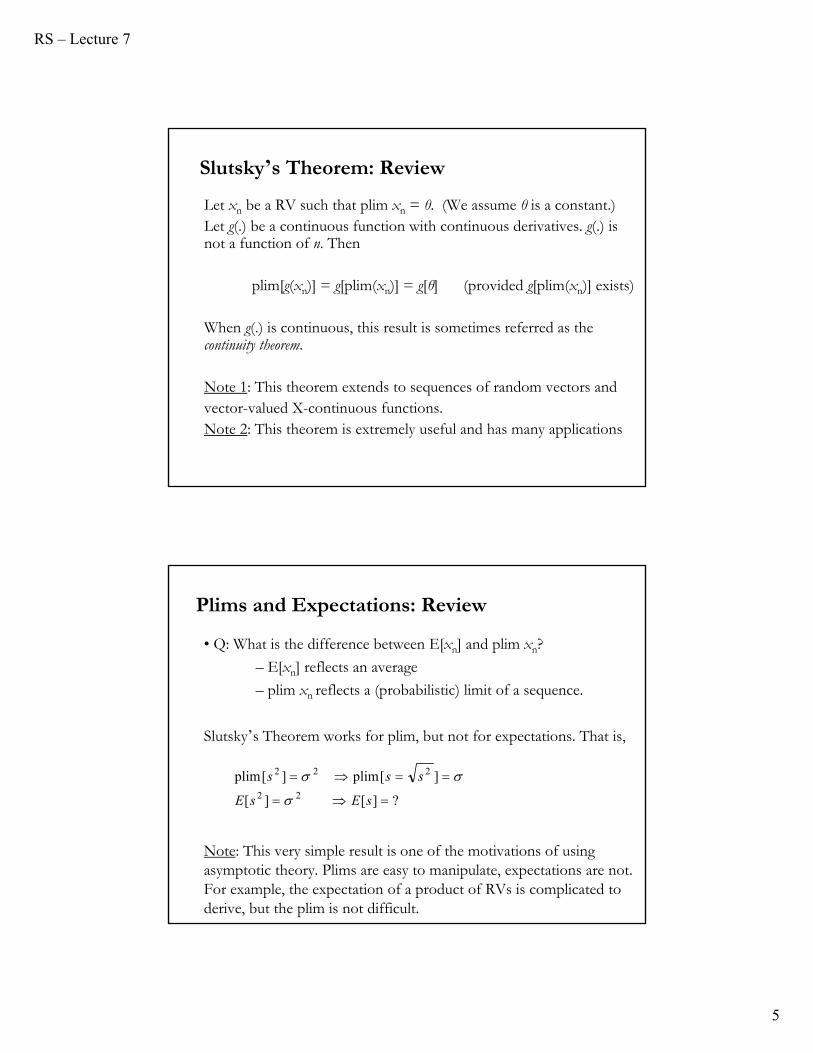
Let xn be a RV such that plim xn = θ. (We assume θ is a constant.)Let g(.) be a continuous function with continuous derivatives. g(.) is not a function of n. Then
plim[g(xn)] = g[plim(xn)] = g[θ] (provided g[plim(xn)] exists)
When g(.) is continuous, this result is sometimes referred as the continuity theorem.
Note 1: This theorem extends to sequences of random vectors andvector-valued X-continuous functions.Note 2: This theorem is extremely useful and has many applications
Plims and Expectations: Review
• Q: What is the difference between E[xn] and plim xn?
– E[xn] reflects an average
– plim xn reflects a (probabilistic) limit of a sequence.
Slutsky’s Theorem works for plim, but not for expectations. That is,
Note: This very simple result is one of the motivations of using asymptotic theory. Plims are easy to manipulate, expectations are not. For example, the expectation of a product of RVs is complicated to derive, but the plim is not difficult.
?][][
][plim][plim22
222
sEsE
sss
RS – Lecture 7
6
Properties of plims: Review
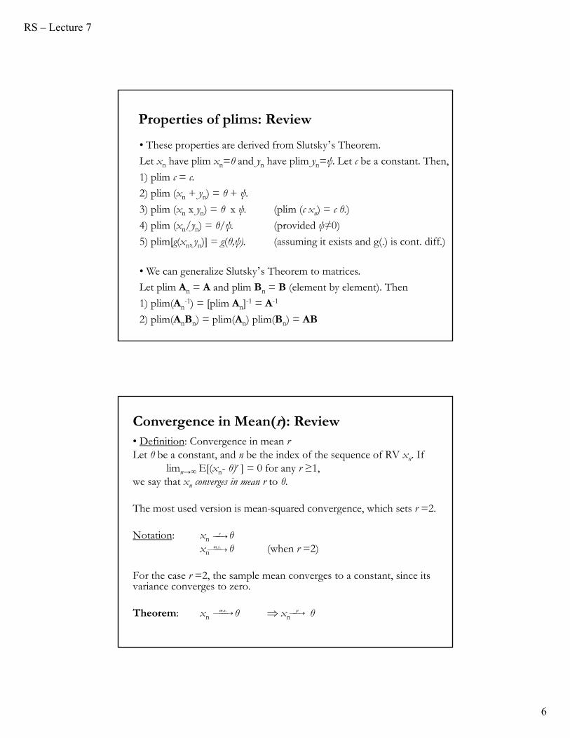
• These properties are derived from Slutsky’s Theorem.
Let xn have plim xn=θ and yn have plim yn=ψ. Let c be a constant. Then,
1) plim c = c.
2) plim (xn + yn) = θ + ψ.
3) plim (xn x yn) = θ x ψ. (plim (c xn) = c θ.)
4) plim (xn/yn) = θ/ψ. (provided ψ≠0)
5) plim[g(xn, yn)] = g(θ,ψ). (assuming it exists and g(.) is cont. diff.)
• We can generalize Slutsky’s Theorem to matrices.
Let plim An = A and plim Bn = B (element by element). Then
1) plim(An-1) = [plim An]-1 = A-1
2) plim(AnBn) = plim(An) plim(Bn) = AB
• Definition: Convergence in mean rLet θ be a constant, and n be the index of the sequence of RV xn. If
limn→∞ E[(xn- θ)r ] = 0 for any r ≥1, we say that xn converges in mean r to θ.
The most used version is mean-squared convergence, which sets r =2.
Notation: xn θxn θ (when r =2)
For the case r =2, the sample mean converges to a constant, since its variance converges to zero.
Theorem: xn θ xn θ
Convergence in Mean(r): Review
r
..sm p
..sm
RS – Lecture 7
7
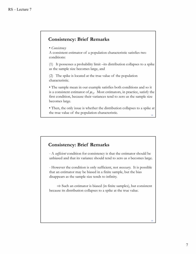
• ConsistencyA consistent estimator of a population characteristic satisfies two conditions:
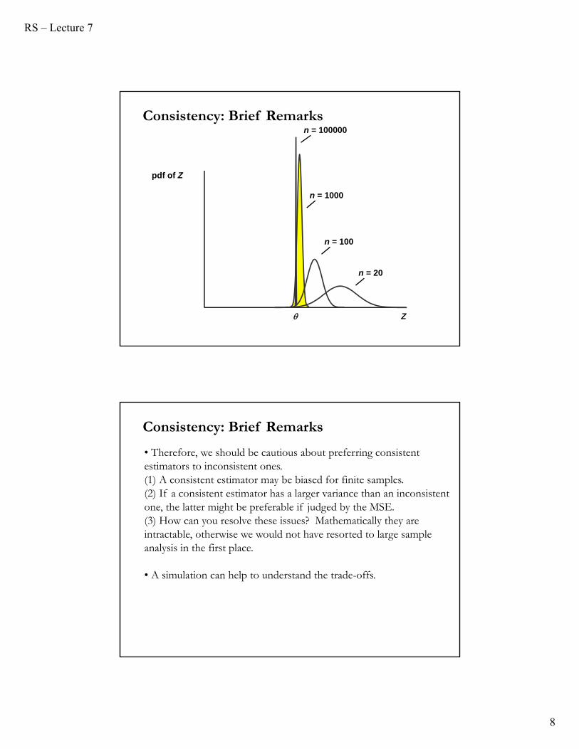
(1) It possesses a probability limit –its distribution collapses to a spike as the sample size becomes large, and
(2) The spike is located at the true value of the population characteristic.
• The sample mean in our example satisfies both conditions and so it is a consistent estimator of X. Most estimators, in practice, satisfy the first condition, because their variances tend to zero as the sample size becomes large.
• Then, the only issue is whether the distribution collapses to a spike at the true value of the population characteristic.
20
Consistency: Brief Remarks
- A sufficient condition for consistency is that the estimator should be unbiased and that its variance should tend to zero as n becomes large.
- However the condition is only sufficient, not necessary. It is possible that an estimator may be biased in a finite sample, but the bias disappears as the sample size tends to infinity.
Such an estimator is biased (in finite samples), but consistent because its distribution collapses to a spike at the true value.
20
Consistency: Brief Remarks
RS – Lecture 7
8
n = 100
n = 1000
n = 20
pdf of Z
Z
n = 100000
Consistency: Brief Remarks
• Therefore, we should be cautious about preferring consistent estimators to inconsistent ones.(1) A consistent estimator may be biased for finite samples.(2) If a consistent estimator has a larger variance than an inconsistent one, the latter might be preferable if judged by the MSE. (3) How can you resolve these issues? Mathematically they are intractable, otherwise we would not have resorted to large sample analysis in the first place.
• A simulation can help to understand the trade-offs.
Consistency: Brief Remarks
RS – Lecture 7
9
• Definition: Almost sure convergence
Let θ be a constant, and n be the index of the sequence of RV xn. If
P[limn→∞ xn= θ] = 1,
we say that xn converges almost surely to θ.
The probability of observing a realization of {xn} that does not converge to θ is zero. {xn} may not converge everywhere to θ, but the points where it does not converge form a zero measure set (probability sense).
Notation: xn θ
This is a stronger convergence than convergence in probability.
Theorem: xn θ xn θ
Almost Sure Convergence: Review
..sa p
..sa
• In almost sure convergence, the probability measure takes into account the joint distribution of {Xn}. With convergence in probability we only look at the joint distribution of the elements of {Xn} that actually appear in xn.
• Strong Law of Large Numbers
We can state the LLN in terms of almost sure convergence:
Under certain assumptions, sample moments converge almost surely to their population counterparts.
This is the Strong LLN.
• From the previous theorem, the Strong LLN implies the (Weak) LLN.
Almost Sure Convergence: Strong LLN
RS – Lecture 7
10
• Versions used in Greene
(i) Khinchine’s Strong LLN.
Assumptions: {Xn}is a sequence of i.i.d. RVs with E[Xn] = μ < ∞.
(ii) Kolmogorov’s Strong LLN.
Assumptions: {Xn}is a sequence of independent. RVs with E[Xn] = μ < ∞and Var[Xn] = σ2 < ∞.
Almost Sure Convergence: Strong LLN
• In econometrics, we often deal with sample means of random functions. A random function is a function that is a random variable for each fixed value of its argument.
• In cross section econometrics, random functions usually take the form of a function g(Z,θ) of a random vector Z and a non-random vector θ.
• For example, consider a Poisson model:
• Let ln λi= Xiβ and denote Zj = (Yj ,Xj). Then,
g(Zi, θ) = –Xiβ + yj ln(Xiβ) – Σi ln(yj), where θ= β
For these functions we can extend the LLN to a Uniform LLN.
Convergence for Random Functions: ULLN
!)|(Pr
i
yi
iii y
eXyYob
ii
RS – Lecture 7
11
• Theorem: Uniform weak LLN (UWLLN)Let {Zj, j = 1,..,n}be a random sample from a k-variate distribution. Let g(z, θ) be a Borel measurable function on Ζ × Θ, where Ζ∈Rk is a Borelset such that P[Zt ∈ Ζ] = 1, and Θ is a compact subset of Rm, such that for each z∈Ζ, g(z,θ) is a continuous function on Θ. Furthermore, let
E[supθ∈Θ |g(Zj , θ)|] < ∞Then,
plim supθ∈Θ |(1/n) Σj g(Zj , θ) – E[g(Z, θ)]| = 0.
• That is, for any fixed θ, the sequence {g(Z1,θ), g(Z2,θ), …} will be a sequence of i.i.d. RVs, such that the sample mean of this sequence converges in probability to E[g(Z,θ)]. This is the pointwise (in θ) convergence.
• Note: The condition that the random vectors Zj are i.i.d. can be relaxed (in Time Series we use strict stationarity & ergodicity).
Convergence for Random Functions: ULLN
Back to CLM: New Assumptions
(1) {xi,εi} i=1, 2, ...., T is a sequence of independent observations.
– X is stochastic, but independent of the process generating .– We require that X have finite means and variances. Similar requirement for , but we also require E[]=0.
(2) Well behaved X:
plim (XX/T) = Q (Q a pd matrix of finite elements)
- Q: Why do we need assumption (2) in terms of a ratio divided by T? Each element of XX matrix is a sum of T numbers. As T , these sums will become large. We divide by T so that the sums will not be too large.
RS – Lecture 7
12
(2) plim (XX/T) = Q (Q a pd matrix of finite elements)
Note: This assumption is not a difficult one to make since the LLN suggests that the each component of XX/T goes to the mean values of XX. We require that these values are finite.
– Implicitly, we assume that there is not too much dependence in X.
Linear Model: New Assumptions
• Now, we have a new set of assumptions in the CLM:
(A1) DGP: y = X + . (A2’) X stochastic, but E[X’ ]= 0 and E[]=0.
(A3) Var[|X] = σ2 IT
(A4’) plim (XX/T) = Q (p.d. matrix with finite elements, rank= k)
• We want to study the large sample properties of OLS:
Q 1: Is b consistent? s2?
Q 2: What is the distribution of b?
Q 3: What about the distribution of the tests: t-tests, F-tests and Wald tests?
Linear Model: New Assumptions
RS – Lecture 7
13
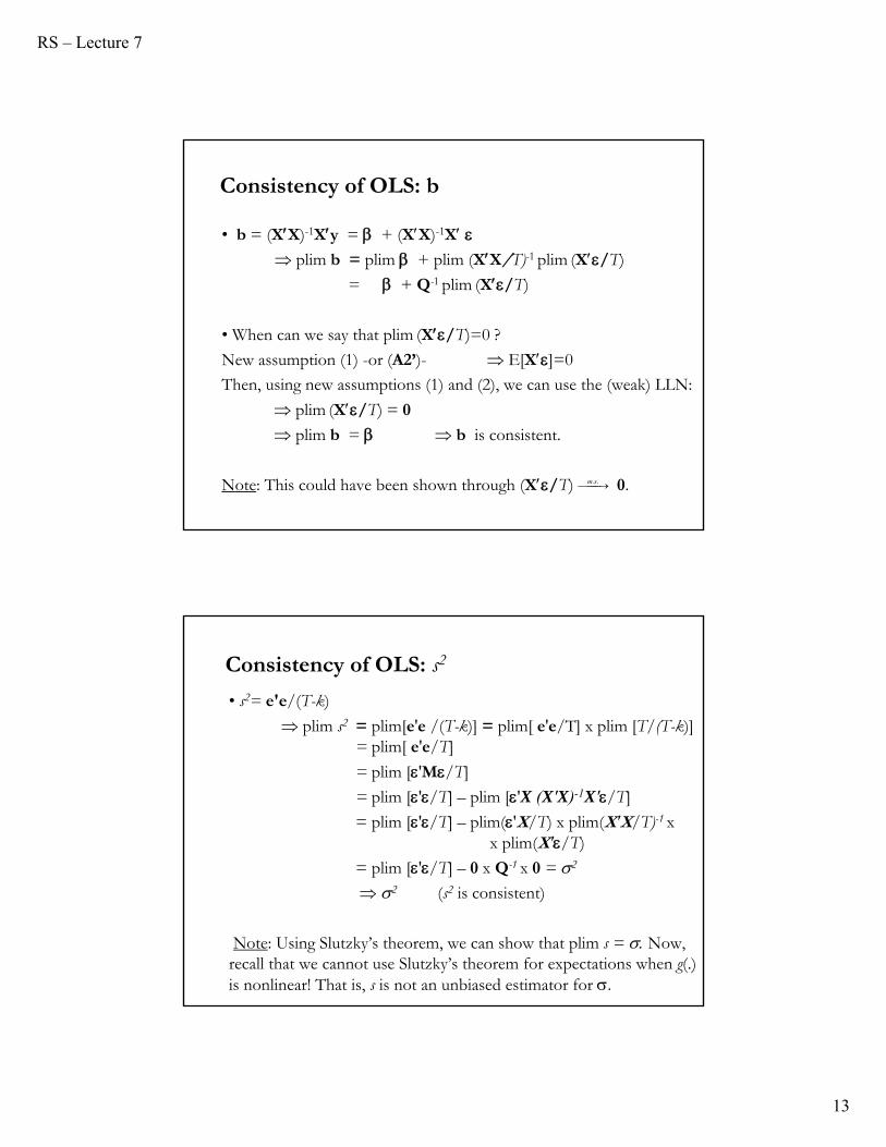
Consistency of OLS: b
• b = (XX)-1Xy = + (XX)-1X plim b = plim + plim (XX/T)-1 plim (X/T)
= + Q-1 plim (X/T)
• When can we say that plim (X/T)=0 ?
New assumption (1) -or (A2’)- E[X]=0
Then, using new assumptions (1) and (2), we can use the (weak) LLN:
plim (X/T) = 0
plim b = b is consistent.
Note: This could have been shown through (X/T) 0. ..sm
Consistency of OLS: s2
• s2= e'e/(T-k)
plim s2 = plim[e'e /(T-k)] = plim[ e'e/T] x plim [T/(T-k)]= plim[ e'e/T]
= plim ['M/T]
= plim ['/T] – plim ['X (X′X)-1X′/T]
= plim ['/T] – plim('X/T) x plim(X′X/T)-1 xx plim(X′/T)
= plim ['/T] – 0 x Q-1 x 0 = 2
2 (s2 is consistent)
Note: Using Slutzky’s theorem, we can show that plim s = Now, recall that we cannot use Slutzky’s theorem for expectations when g(.) is nonlinear! That is, s is not an unbiased estimator for .
RS – Lecture 7
14
Convergence to a Random Variable: Review
• Definition: Limiting DistributionLet xn be a random sequence with cdf Fn(xn). Let x be a random variable with cdf F(x).
When Fn converges to F as n→ ∞, for all points x at which F(x) is continuous, we say that xn converges in distribution to x. The distribution of that random variable is the limiting distribution of xn.
Notation: xn x
Example: The tn statistic converges to a standard normal: tn N(0,1)
Remark: If plim xn = θ (a constant), then Fn(xn) becomes a point.
d
d
Theorem: If xn x and plim yn= c. Then, xn yn c x. That is the limiting distribution of xn yn is the distribution of c x.
Also, xn + yn x +cxn/yn x/c (provided + c≠0.)
d d
d
d
Convergence to a Random Variable: Review
RS – Lecture 7
15
Slutsky’s Theorem for RVs - Review
Let xn converge in distribution to x and let g(.) be a continuous function with continuous derivatives. g(.) is not a function of n. Then,
g(xn) g(x).
Example: tn N(0,1) g(tn) = (tn)2 [N(0,1)]2.
• Extension
Let xn x and g(xn,θ) g(x) (θ: parameter).
Let plim yn=θ (yn is a consistent estimator of θ)
Then, g(xn,yn) g(x).
That is, replacing θ by a consistent estimator leads to the same limiting distribution.
d
dd
dd
d
Extension of Slutsky’s Theorem: Examples
• Example 1: tT statistic
z = T1/2 ( – μ)/σ N(0,1)
tT = T1/2 ( – μ)/sT N(0,1) (where plim sT = σ)
• Example 2: F-statistic for testing restricted regressions.
F = [(e*’e* – e’e)/J]/[e’e/(T – k)]
= [(e*’e* – e’e)/(σ2J)]/[e’e/(σ2(T – k))]
The denominator: e’e/[σ2(T – k)] 1.
Then, the limiting distribution of the F statistic will be given by the limiting distribution of the numerator.
xd
d
p
x
RS – Lecture 7
16
The CLT: Review
• The CLT states conditions for the sequence of RV {xT} under which the mean or a sum of a sufficiently large number of xi’s will be approximately normally distributed.
CLT: Under some conditions, z = T1/2 ( – μ)/σ N(0,1)
• It is a general result. When sums of random variables are involved, eventually (sometimes after transformations) the CLT can be applied.
x d
• Two popular versions in Greene, used in economics and finance:
Lindeberg-Levy: {xn} are i.i.d., with finite μ and finite σ2.
Lindeberg-Feller: {xn} are independent, with finite μi, σi2<∞,
Sn =Σi xi, sn2= Σi σi
2 and for ε>0,
Note:
Lindeberg-Levy assumes random sampling – observations are i.i.d.,with the same mean and same variance.
Lindeberg-Feller allows for heterogeneity in the drawing of the observations --through different variances. The cost of this more general case: More assumptions about how the {xn} vary.
0)()(1
lim1 ||
2
2
n
i sx
iiin
n
nii
dxxfxs
The CLT: Review
RS – Lecture 7
17
Asymptotic Distribution of OLS
• b = (XX)-1Xy = + (XX)-1X Using Slutzky’s theorem for RV, we know the limiting distribution of b is not affected by replacing (X’X) by its plim. That is, we examine the limiting distribution of
+ Q-1 X/T
• Notice b β. But, it has no distribution! It is O(1/T).We need to do a stabilizing transformation –i.e., the moments do not depend on T. Steps:(1) Stabilize the variance: Var[T b] ~ σ2Q-1 is O(1)(2) Stabilize the mean: E[T (b – β)] = 0
Now, we have a RV, T (b – β), with finite mean and variance .
p
• b = (XX)-1Xy = + (XX)-1XThe stabilizing transformation of b gives us:
T (b - β) = T (XX)-1X’ = T (XX/T)-1(X’ /T)
The limiting behavior of T (b - β) is the same as that of
T Q-1(X/T)
Q is a fixed matrix. Asymptotic behavior depends on the RV
T (X/T)
• T (Xε/T) = T ixiεi/T = T [1/T iwi] = T
is a sample mean of independent observations.
Asymptotic Distribution of OLS
w
w
RS – Lecture 7
18
• T (Xε/T)= T ixiεi/T = T [1/T iwi] = T
is a sample mean of independent observations.
• Under the new assumptions, 0 (already shown).
• Since Var[xiεi] = σ2xixi Var[ ] σ2Q/T
Var[T ] σ2Q
• We can apply the Lindeberg-Feller CLT: T N(0, σ2Q)
T N(0, σ2Q)
Q-1T N(0, σ2 Q-1 Q Q-1) = N(0, σ2Q-1)
T (b – β) N(0, σ2Q-1)
b N(β, (σ2/T)Q-1)
Asymptotic Distribution of OLS
w
w
w p
w p
pw
dw
w
d
dw
d
a
Asymptotic Results
• How ‘fast’ does b converges to β?
Asy.Var[b] = σ2/T Q-1 is O(1/T)
– Convergence is at the rate of 1/T –usual square root rate
– T b has variance of O(1)
• Distribution of b does not depend on normality of ε
• Estimator of the Asy Var[b]=(σ2/T)Q-1 is (s2/T) (XX/T)-1. (The degrees of freedom correction is irrelevant. It may matter for small sample behavior.)
• Slutsky's theorem and the delta method apply to functions of b.
RS – Lecture 7
19
Test Statistics
• We have established the asymptotic distribution of b. We now turn to the construction of test statistics, which are functions of b.
• Again, we know that if (A5) |X ~N(0, σ2IT), the Wald statistic
F[J,n-K] = (1/J)(Rb - q)’[R s2(XX)-1R]-1(Rb - q) ~ FJ,T-k
• Q: What is the distribution of F when (A5) is no longer assumed? Again, we will study the distribution of test statistics when T→∞.
Wald Statistics: Cheat sheet
• Recall these results:
- A square of a N(0,1) RV ~ 12
- If z~N[,2]. Then [(z – )/]2 ~ χ12 (normalized distance (in SD units) between z and .)
- Suppose zT is not normally distributed, with E[zT]= & Var[zT]= 2. Then, under certain assumption, the limiting distribution of zT is normal (CLT):
T = (zT - )/ N[0,1].
- If the preceding holds T2 = [(zT – )/]2 1
2.
- Let be unknown. We use sT such that plim sT = .
tT = [(zT – )/sT] N(0,1) (Slutzky’s theorem)
d
d
d
RS – Lecture 7
20
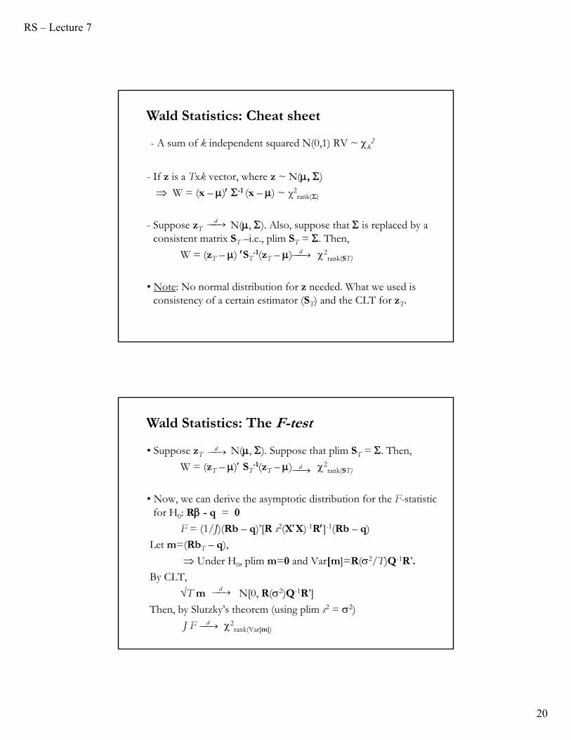
- A sum of k independent squared N(0,1) RV ~ k2
- If z is a Txk vector, where z ~ N(, )
W = (x – ) -1 (x – ) ~ χ2rank(Σ)
- Suppose zT N(, ). Also, suppose that is replaced by a consistent matrix ST –i.e., plim ST = . Then,
W = (zT – ) ST-1(zT – ) 2
rank(ST)
• Note: No normal distribution for z needed. What we used is consistency of a certain estimator (ST) and the CLT for zT.
d
d
Wald Statistics: Cheat sheet
• Suppose zT N(, ). Suppose that plim ST = . Then,
W = (zT – ) ST-1(zT – ) 2
rank(ST)
• Now, we can derive the asymptotic distribution for the F-statistic for H0: R - q = 0
F = (1/J)(Rb – q)’[R s2(XX)-1R]-1(Rb – q)
Let m=(RbT – q),
Under H0, plim m=0 and Var[m]=R(2/T)Q-1R’.
By CLT,
T m N[0, R(2)Q-1R’]
Then, by Slutzky’s theorem (using plim s2 = 2)
J F 2rank(Var[m])
d
d
d
d
Wald Statistics: The F-test
RS – Lecture 7
21
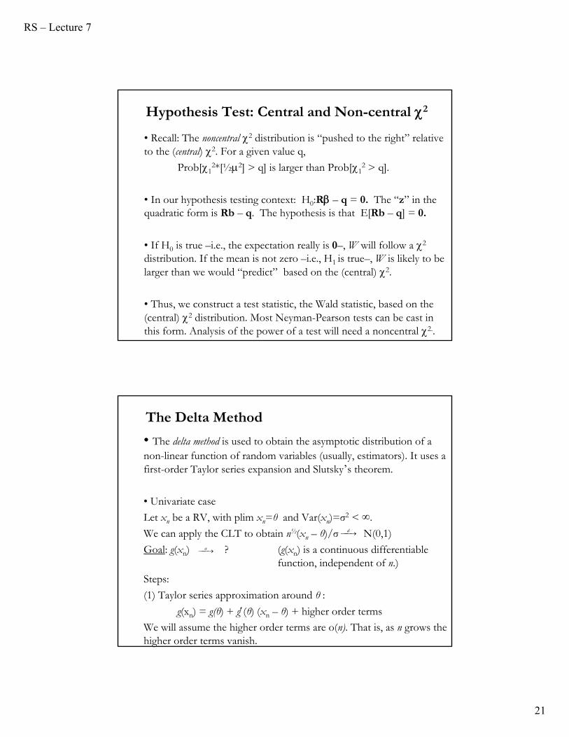
Hypothesis Test: Central and Non-central 2
• Recall: The noncentral 2 distribution is “pushed to the right” relative to the (central) 2. For a given value q,
Prob[12*[½2] > q] is larger than Prob[1
2 > q].
• In our hypothesis testing context: H0:R – q = 0. The “z” in the quadratic form is Rb – q. The hypothesis is that E[Rb – q] = 0.
• If H0 is true –i.e., the expectation really is 0–, W will follow a 2
distribution. If the mean is not zero –i.e., H1 is true–, W is likely to be larger than we would “predict” based on the (central) 2.
• Thus, we construct a test statistic, the Wald statistic, based on the (central) 2 distribution. Most Neyman-Pearson tests can be cast in this form. Analysis of the power of a test will need a noncentral 2..
The Delta Method
• The delta method is used to obtain the asymptotic distribution of a non-linear function of random variables (usually, estimators). It uses a first-order Taylor series expansion and Slutsky’s theorem.
• Univariate case
Let xn be a RV, with plim xn=θ and Var(xn)=σ2 < ∞.
We can apply the CLT to obtain n½(xn – θ)/σ N(0,1)
Goal: g(xn) ? (g(xn) is a continuous differentiable function, independent of n.)
Steps:
(1) Taylor series approximation around θ :
g(xn) = g(θ) + g(θ) (xn – θ) + higher order terms
We will assume the higher order terms are o(n). That is, as n grows the higher order terms vanish.
a
d
RS – Lecture 7
22
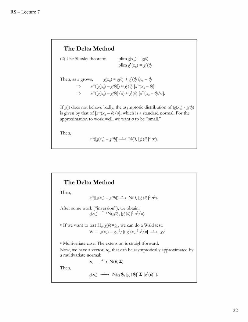
(2) Use Slutsky theorem: plim g(xn) = g(θ)plim g’(xn) = g’(θ)
Then, as n grows, g(xn) g(θ) + g(θ) (xn – θ)
n½([g(xn) – g(θ)]) g(θ) [n½(xn – θ)].
n½([g(xn) – g(θ)]/σ) g(θ) [n½(xn – θ)/σ].
If g(.) does not behave badly, the asymptotic distribution of (g(xn) - g(θ)) is given by that of [n½(xn – θ)/σ], which is a standard normal. For the approximation to work well, we want σ to be “small.”
Then,n½([g(xn) – g(θ)]) N(0, [g(θ)]2 σ2).a
The Delta Method
Then,n½([g(xn) – g(θ)]) N(0, [g(θ)]2 σ2).
After some work (“inversion”), we obtain:g(xn) N(g(θ), [g(θ)]2 σ2/n).
• If we want to test H0: g(θ)=g0, we can do a Wald test:W = [g(xn) – g0]2/[([g(xn]2 s2/n] χ1
2
• Multivariate case: The extension is straightforward.Now, we have a vector, xn, that can be asymptotically approximated by a multivariate normal:
xn N(θ, Σ)Then,
g(xn) N(g(θ), [g(θ)]’ Σ [g(θ)] ).
The Delta Method
a
a
a
a
a
RS – Lecture 7
23
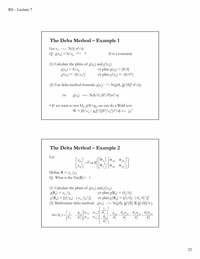
Let xn N(θ, σ2/n)Q: g(xn) = δ/xn ? (δ is a constant)
(1) Calculate the plims of g(xn) and g’(xn):g(xn) = δ/xn plim g(xn) = (δ/θ)g’(xn) = -(δ/xn
2) plim g’(xn) = -(δ/θ 2)
(2) Use delta method formula: g(xn) N(g(θ), [g(θ)]2 σ2/n).
g(xn) N(δ/θ, (δ2/θ4)σ2/n)
• If we want to test H0: g(θ)=g0, we can do a Wald test:W = [δ/xn – g0]2/[(δ2/xn
4)s2/n] χ12
a
a
a
a
The Delta Method – Example 1
a
Let
Define R = xn /yn.Q: What is the Var(R)= ?
(1) Calculate the plims of g(xn) and g’(xn):g(Rn) = xn /yn plim g(Rn) = (θx/θy)g’(Rn) = [(1/yn) (-xn /yn
2 )] plim g’(Rn) = [(1/θy) (-θx/θy2 )]’
(2) Multivariate delta method: g(xn) N(g(θ), [g(θ)]’ Σ [g(θ)]/n ).a
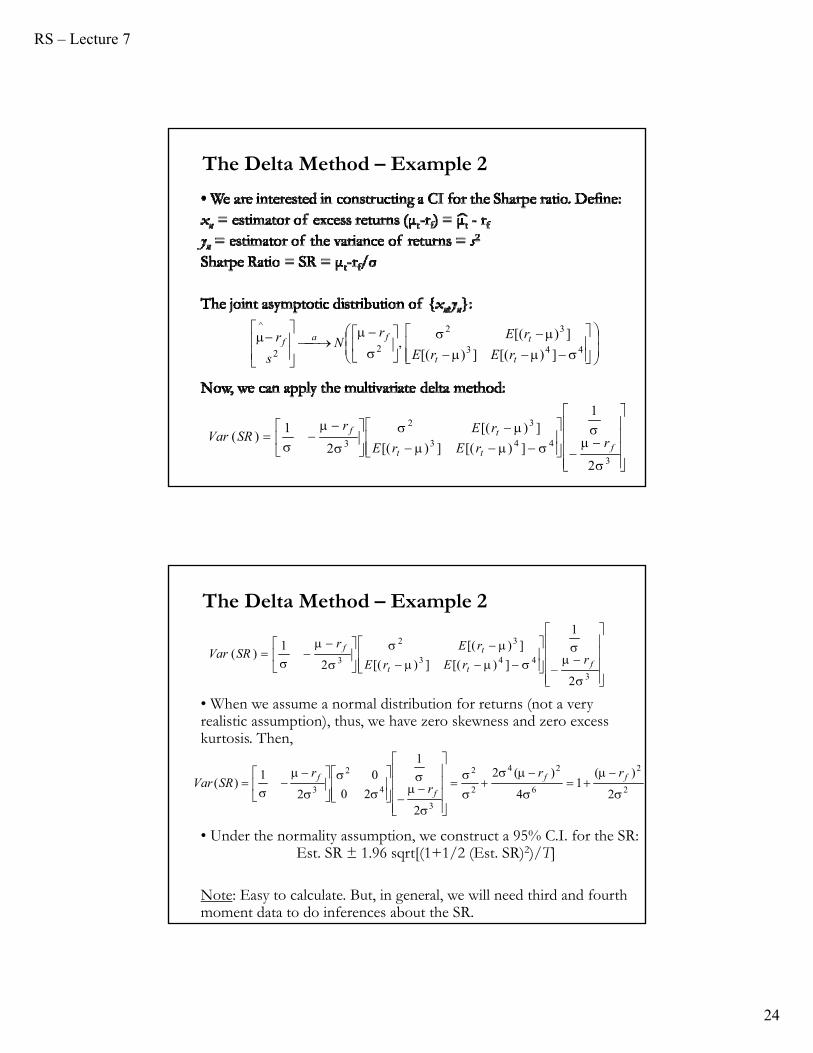
The Delta Method – Example 2
yyyx
xyxx
y
xa
n
n Ny
x,
4
2
332
2
2
1
1)(
y
yyx
y
xyx
y
xyx
y
xx
y
x
y
yyyx
xyxx
y
x
ynRVar
RS – Lecture 7
24
The Delta Method – Example 2
443
32
22
^
])[(])[(
])[(,
tt
tfaf
rErE
rErN
s
r
3
443
32
3
2
1
])[(])[(
])[(
2
1)(
ftt
tf
rrErE
rErSRVar
• When we assume a normal distribution for returns (not a very realistic assumption), thus, we have zero skewness and zero excess kurtosis. Then,
The Delta Method – Example 2
3
443
32
3
2
1
])[(])[(
])[(
2
1)(
ftt
tf
rrErE
rErSRVar
2
2
6
24
2
2
3
4
2
3 2
)(1
4
)(2
2
1
20
0
2
1)(
ff
f
f rrr
rSRVar
• Under the normality assumption, we construct a 95% C.I. for the SR: Est. SR ± 1.96 sqrt[(1+1/2 (Est. SR)2)/T]
Note: Easy to calculate. But, in general, we will need third and fourth moment data to do inferences about the SR.
RS – Lecture 7
25
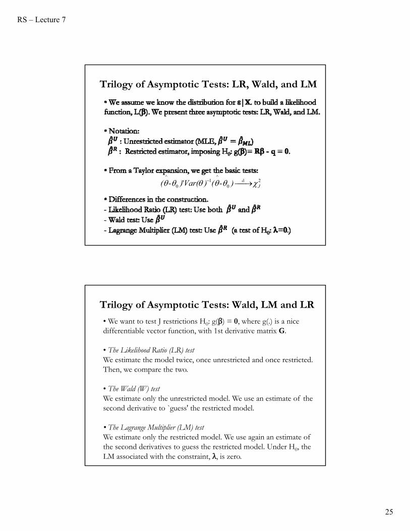
Trilogy of Asymptotic Tests: LR, Wald, and LM
20
^1
0
^
' J)-()Var()-( d
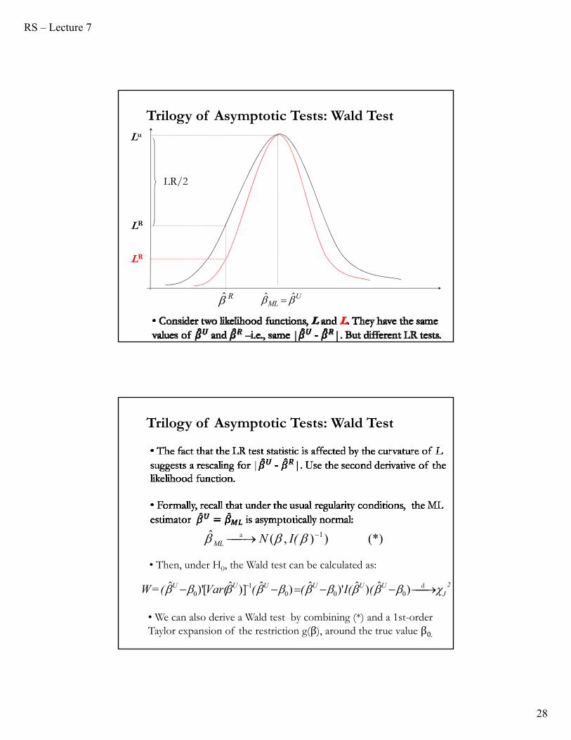
Trilogy of Asymptotic Tests: Wald, LM and LR
• We want to test J restrictions H0: g(β) = 0, where g(.) is a nice differentiable vector function, with 1st derivative matrix G.
• The Likelihood Ratio (LR) testWe estimate the model twice, once unrestricted and once restricted.Then, we compare the two.
• The Wald (W) testWe estimate only the unrestricted model. We use an estimate of thesecond derivative to `guess' the restricted model.
• The Lagrange Multiplier (LM) testWe estimate only the restricted model. We use again an estimate ofthe second derivatives to guess the restricted model. Under H0, theLM associated with the constraint, λ, is zero.
RS – Lecture 7
26
Lu
LR
UML ˆˆ R̂
LR/2
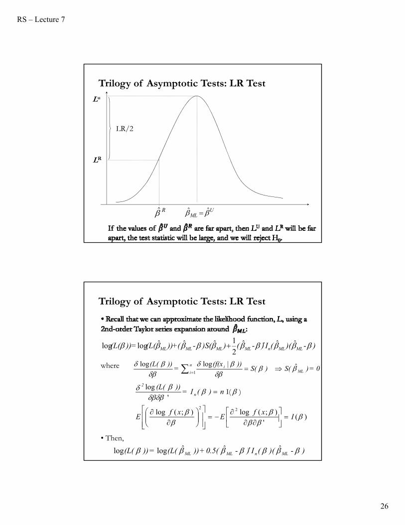
Trilogy of Asymptotic Tests: LR Test
)-)((I)-())S(-(+))(L(=))(L( MLMLnMLMLMLML ˆˆˆ2
1ˆˆˆloglog
0=)S()S())(f(x
=))(L(
ML
n
ii
ˆ|loglog
1
)('
);(log);(log
'
log
22
Ixf
Exf
E
n)(I= ))(L(
n
2
)I(
Trilogy of Asymptotic Tests: LR Test
)-)((I)-0.5(+))(L(=))(L( MLnMLML ˆˆˆloglog
where
• Then,
RS – Lecture 7
27
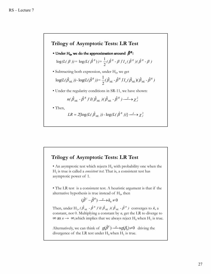
)-((I)-(=))(L(-))(L( RMLMLn
RML
RML ˆˆ)ˆˆˆ
2
1ˆlogˆlog
• Under the regularity conditions in SR-11, we have shown:
2ˆˆˆ'ˆˆJ
RMLML
RML )-)(I()-n( d
2]ˆlogˆ[log JR
ML ))(L(-))(L(2LR d
• Then,
Trilogy of Asymptotic Tests: LR Test
)-)((I)-(+)(L(=))(L( RRn
RR ˆˆˆ2
1)ˆloglog
• Subtracting both expression, under H0, we get
0)ˆˆ( 0 kRU p
Trilogy of Asymptotic Tests: LR Test
• An asymptotic test which rejects H0 with probability one when the H1 is true is called a consistent test. That is, a consistent test has asymptotic power of 1.
• The LR test is a consistent test. A heuristic argument is that if the alternative hypothesis is true instead of H0, then
Then, under H1, converges to k, a constant, not 0. Multiplying a constant by n, get the LR to diverge to ∞asn → ∞,which implies that we always reject H0 when H1 is true.
Alternatively, we can think of driving the divergence of the LR test under H0 when H1 is true.
)-)(I()-( RMLML
RML ˆˆˆ'ˆˆ
0)()ˆ( 0 gg U p
RS – Lecture 7
28
Lu
LR
UML ˆˆ R̂
LR/2
Trilogy of Asymptotic Tests: Wald Test
LR
(*))),(ˆ 1 I(NMLa
• Then, under H0, the Wald test can be calculated as:
• We can also derive a Wald test by combining (*) and a 1st-order Taylor expansion of the restriction g(β), around the true value β0.
J2UUUUUU (I(((Var((=W d)ˆ)ˆ)'ˆ)ˆ)]ˆ[)'ˆ
0001
0
Trilogy of Asymptotic Tests: Wald Test
RS – Lecture 7
29
• We can also derive a Wald test by combining (*) and a 1st-order Taylor expansion of the restriction g(β), around the true value β0:
Trilogy of Asymptotic Tests: Wald Test
)o)-(G+g(=)g( UU 1(ˆ')ˆ00
• A little bit of algebra and (*) deliver:
)',0())ˆ( 100 G)I(GNg()g(n dU
• Under H0: g(β0)=0, we form the usual quadratic form for a Wald test:
211 ˆ]ˆ'['ˆJ
UUU )g(G)I(G)g(n d
Lu
LR
UML ˆˆ R̂
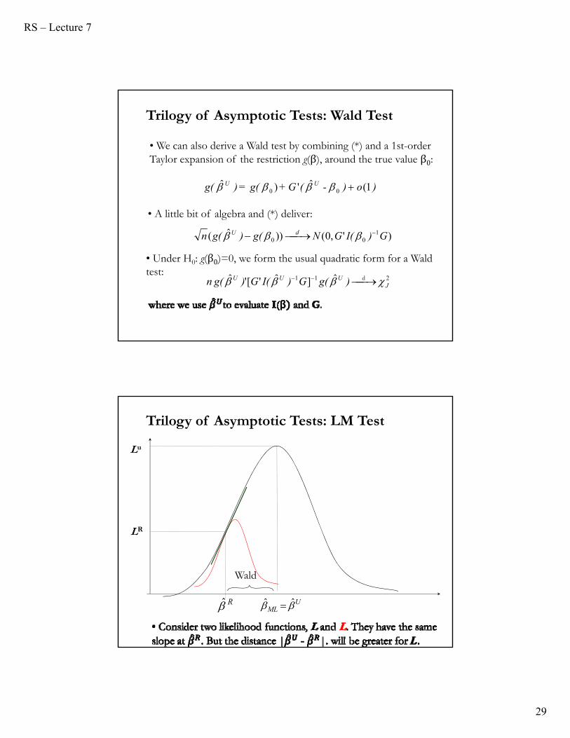
Trilogy of Asymptotic Tests: LM Test
Wald
RS – Lecture 7
30
Trilogy of Asymptotic Tests: LM Test
)' 0
^1
0
^
-()Var()-(
• Recall the score function, S(β) N(0, nI(β)). • The LM (score) test is based on S(β). Under H0, S(βR)=0. Then,
J2RRR S(I(S(
n=LM d))][)'
1 1
This expression looks like an R2 from the regression of 1 on S(β).
a
Trilogy of Asymptotic Tests: LM Test
n
iin
iiin
ii ))(f(x))(f(x))(f(x
n
))(f(x
n=LM
1
1
11 '
|log
'
|log|log1
'
|log1
x
RS – Lecture 7
31
• The (uncentered) R2:ii
iXXXXi=R
'
')'(' 12
• Then, LM = n R2, where R2 is calculated from a regression of a vector of ones on the scores. (This version of the LM test may be referred as Engle’s LM test.)
Example: 0)( 1t21tt g+),,Xf(=Y to subject
where β1 is a subset of parameters restricted by g(β1) =0 (G is the 1st derivative of this restriction).
Trilogy of Asymptotic Tests: LM Test
1
2
][
*
G)GE(=)I(
eG=)S(
2-1
1
• Then,
e*: estimated errors from the restricted model
• The LM test becomes: LM = σ-2 e*’G{σ-2 E[G’G]}-1 σ-2 G’e*
If E[G’G] = G’G LM = σ-2 e*’e*,
with the interpretation as TR2 from a regression of e* on G. This is used in many tests for serial correlation, heteroskedasticity, etc.
Trilogy of Asymptotic Tests: LM Test
Example: Testing for serial correlationSuppose
ttt u+=
+X=Y
1
H0: ρ=0 (no serial correlation).
To calculate the Engle’s LM test we need e*(residuals under ρ=0) and G.
RS – Lecture 7
32
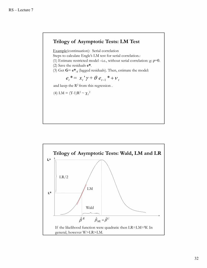
Example(continuation): Serial correlationSteps to calculate Engle’s LM test for serial correlation.:(1) Estimate restricted model –i.e., without serial correlation: g: ρ=0.(2) Save the residuals e*. (3) Get G= e*-1 (lagged residuals). Then, estimate the model:
tttt e+x=e *'* 1
and keep the R2 from this regression .
(4) LM = (T-1)R2 ~ 12
Trilogy of Asymptotic Tests: LM Test
If the likelihood function were quadratic then LR=LM=W. In general, however W>LR>LM.
Lu
LR
UML ˆˆ R̂
LR/2
Wald
LM
Trilogy of Asymptotic Tests: Wald, LM and LR
RS – Lecture 7
33
• The three tests have the same asymptotic distribution: Equivalent as T →∞. Thus, they are expected to give similar results in large samples.
• Their small-sample properties are not known. Simulation studies suggest that the likelihood ratio test may be better in small samples.
• The three tests are consistent, pivotal tests.
Trilogy of Asymptotic Tests: LM Test
Asymptotic Tests: Small sample behavior?
• The p-values from asymptotic tests are approximate for small samples. We worry that tests based on them may over-reject in small samples (or under-reject). The conclusions may end up being too liberal (or too conservative).
• Whether they over-reject or under-reject, and how severely, depends on many things:
(1) Sample size, T.
(2) Distribution of the error terms, .(3) The number of regressors, k, and their properties
(4) The relationship between the error terms and the regressors.
• A simulation can help.
RS – Lecture 7
34
Definition: Pivot Test
A pivot is a statistic whose sampling distribution does not depend on unknown parameters. A test whose distribution does not depend on unknown parameters is called a pivot test.
Example: Suppose you draw X from a N(μ, σ2).
Asymptotic theory implies that is asymptotically N(μ, σ2/N).
This statistic is not asymptotically pivotal statistic because it depends
on an unknown parameter, σ2 (even if you specify μ0 under H0).
On the other hand, the t-statistic, t = ( - μ0)/s is asymptotically N(0, 1). This is asymptotically pivotal since 0 and 1 are known!
Pivot Tests: Review
_
x
_
x
• Most statistics are not asymptotically pivotal. Popular test statistics in econometrics, however, are asymptotically pivotal. For example, Wald, LR and LM tests are distributed as χ2 with known df.
• Keep in mind that in finite samples, most tests are not still asymptotically pivotal in finite samples.
• Under the usual assumptions, the t = (b – )/SE(b) is an example of a pivotal statistic: t ~ tT-k, which does not depend on .
Note: These functions depend on the parameters, but the distribution is independent of the parameters.
Pivot Tests: Review
RS – Lecture 7
35
• Recall the Fundamental Theorem of Statistics:
The empirical cdf → true CDF.
• Then, if we knew that a certain test statistic was pivotal but did not know how it was distributed, we could select any DGP in H0 and generate simulated samples from it.
Trick: Simulation to get the empirical cdf of a statistic. Apply FTS. Sample from our ED to collect B samples of size T.
• The simulated samples can be used to construct a C.I., which easily allows us to test a H0.
Bootstrap: Review
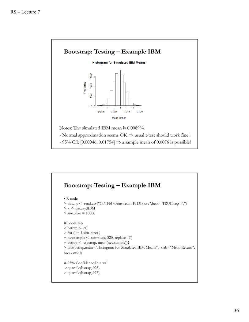
Bootstrap: Testing – Example IBM
• We want to test if IBM has an average return equal to the market,proxied by the S&P 500. H0: μIBM= μMarket = 0.76% monthly (or 9.5% annualized, based on 1928-2015 data).
We have monthly data from 1990: Jan to 2016: August (T=320). Theaverage IBM return was 0.9%. Let’s do a bootstrap to check thesampling distribution of IBM returns.
Steps:(1) Draw B = 10,000 bootstrap subsamples of size T = 320.(2) For each subsample, calculate the observed sample mean, ̅ j*.(3) Draw a histogram
From the histogram, it is straightforward to build a (1-α)% C.I. and check if the market return (0.76%) falls within it.
RS – Lecture 7
36
Notes: The simulated IBM mean is 0.0089%.
- Normal approximation seems OK usual t-test should work fine!.
- 95% C.I: [0.00046, 0.01754] a sample mean of 0.0076 is possible!
Bootstrap: Testing – Example IBM
Bootstrap: Testing – Example IBM
• R-code> dat_xy <- read.csv("C:/IFM/datastream-K-DIS.csv",head=TRUE,sep=",")> x <- dat_xy$IBM> sim_size = 10000
# bootstrap> bstrap <- c()> for (i in 1:sim_size){+ newsample <- sample(x, 320, replace=T)+ bstrap <- c(bstrap, mean(newsample))}> hist(bstrap,main="Histogram for Simulated IBM Means", xlab="Mean Return", breaks=20)
# 95% Confidence Interval>quantile(bstrap,.025)
> quantile(bstrap,.975)
RS – Lecture 7
37
• Suppose we are interested in testing in the CLM, H0: β2 =β2,0.
We use a t-statistic: t = (b2 -β2,0)/SE(b2), which is asymptotically pivotal (N(0,1) asymptotic distribution).
• Bootstrapping can provide some finite sample correction (refinement), providing more accurate estimates of the t-test.
Steps:
(1) Draw B (say, 999) bootstrap subsamples of size T from your data. Denote the subsamples as wj*={yj, xj}, j = 1, 2, …, B.
(2) For each subsample calculate the observed t*j=(b2,j - β2,0)/SE(b2,j).
(3) Sort these B estimates from smallest to largest.
Bootstrap critical values
• In the last step, we sort the B tj* estimates from smallest to largest.
• For an (upper) one-tailed test the bootstrap critical value (at level α) is the “upper αth quantile” of the B estimates of tj*. For example, if B = 999, choose the critical value of t at the 5% level as t950*.
• For two-sided tests, there are two possibilities.
(1) A non-symmetrical or equal-tailed test has the same number of bootstrapped estimates in the two tails, which may implies that the critical values for the upper and lower tails are not necessarily equal in
absolute value. For example, for inference at the 5% significance level |t25*| may not be equal to |t975*|.
Bootstrap critical values
RS – Lecture 7
38
(2) In contrast, a symmetric test orders the tj*’s in terms of their absolute values and the critical value is the single value in absolute value terms. For example, with B=999 and a 5% significance level, order all 999 tj*’s in terms of their absolute value from smallest to the largest. Pick the one that is 50th from the top and compare that to |t|.
Note: An alternative (but “unrefined”) method to test H0 is to just use the bootstrapped standard errors to compute
t = (b2 – β2,0)/SEboot(b2).
Bootstrap critical values
• Another “unrefined” method is not to calculate any standard errors at all. We use the B b2*’s estimates to build a confidence interval.
Suppose we are interested in a 2-sided test.
Steps:
(1) As usual, calculate B estimates of b2, call them b2,1*, … , b2,B*.
(2) At the α% significance level, cut out the bottom (α/2)% and the top (α/2)% estimates of β2
(3) Reject H0 if β2,0 falls outside this range.
This method is called the percentile method for conducting hypothesis tests.
Bootstrap critical values
RS – Lecture 7
39
• Recall that the p-value is the probability, under H0, of obtaining a more extreme (or equal to) result than what was actually observed.
• We compute p-values through a simulation for a test statistic, ,with observed value . ( follows a distribution under H0; is a realization.)
(1) Choose any DGP in H0, and draw B (say, 999) samples of size Tfrom it. Denote the simulated samples as yj*, j = 1, 2, …, B.
(2) For each simulated sample calculate the observed *j.
(3) Count the number of times the simulated values (*j's) exceeds the observed value . Divide by B. This is the bootstrapped p-value:
Bootstrap p-values
• Since the EDF converges to the true CDF, it follows that, if B were infinitely large, this procedure would yield an exact test.
• Simulating a pivotal statistic is called a Monte Carlo test; Dufour and Khalaf (2001) provides a more detailed introduction and references.
Bootstrap p-values
RS – Lecture 7
40
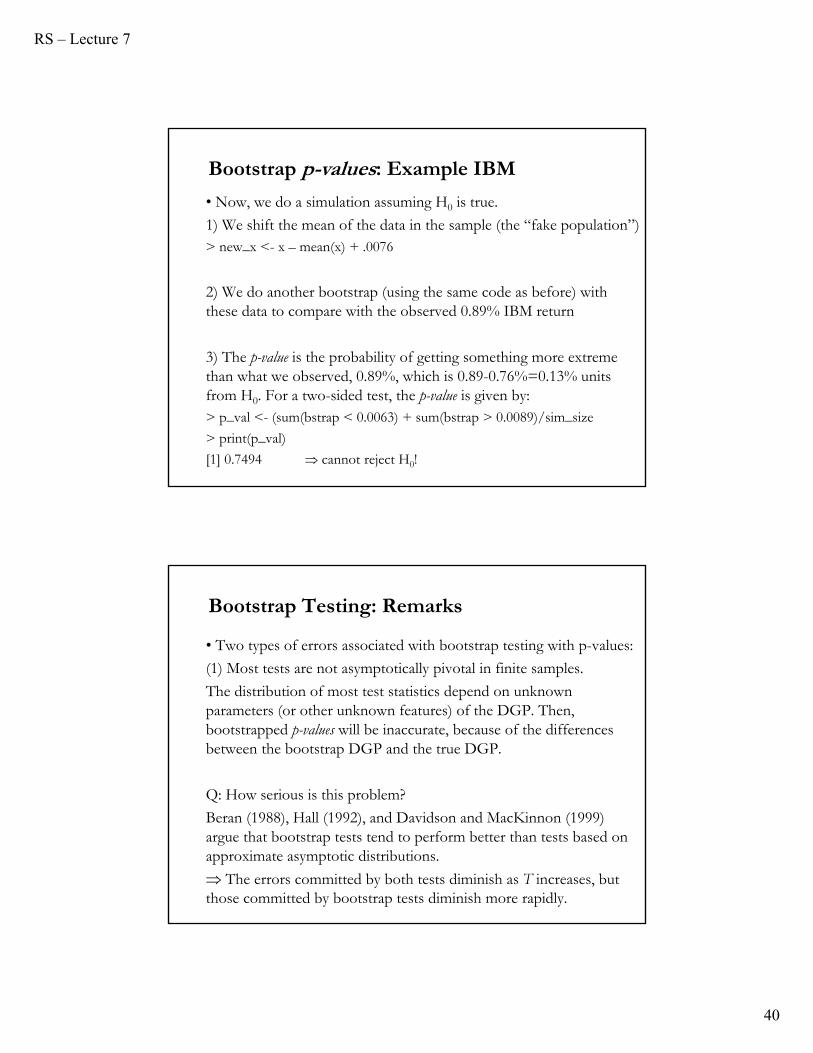
• Now, we do a simulation assuming H0 is true.
1) We shift the mean of the data in the sample (the “fake population”)> new_x <- x – mean(x) + .0076
2) We do another bootstrap (using the same code as before) with these data to compare with the observed 0.89% IBM return
3) The p-value is the probability of getting something more extreme than what we observed, 0.89%, which is 0.89-0.76%=0.13% units from H0. For a two-sided test, the p-value is given by:> p_val <- (sum(bstrap < 0.0063) + sum(bstrap > 0.0089)/sim_size
> print(p_val)
[1] 0.7494 cannot reject H0!
Bootstrap p-values: Example IBM
Bootstrap Testing: Remarks
• Two types of errors associated with bootstrap testing with p-values:
(1) Most tests are not asymptotically pivotal in finite samples.
The distribution of most test statistics depend on unknown parameters (or other unknown features) of the DGP. Then, bootstrapped p-values will be inaccurate, because of the differences between the bootstrap DGP and the true DGP.
Q: How serious is this problem?
Beran (1988), Hall (1992), and Davidson and MacKinnon (1999) argue that bootstrap tests tend to perform better than tests based on approximate asymptotic distributions.
The errors committed by both tests diminish as T increases, but those committed by bootstrap tests diminish more rapidly.
RS – Lecture 7
41
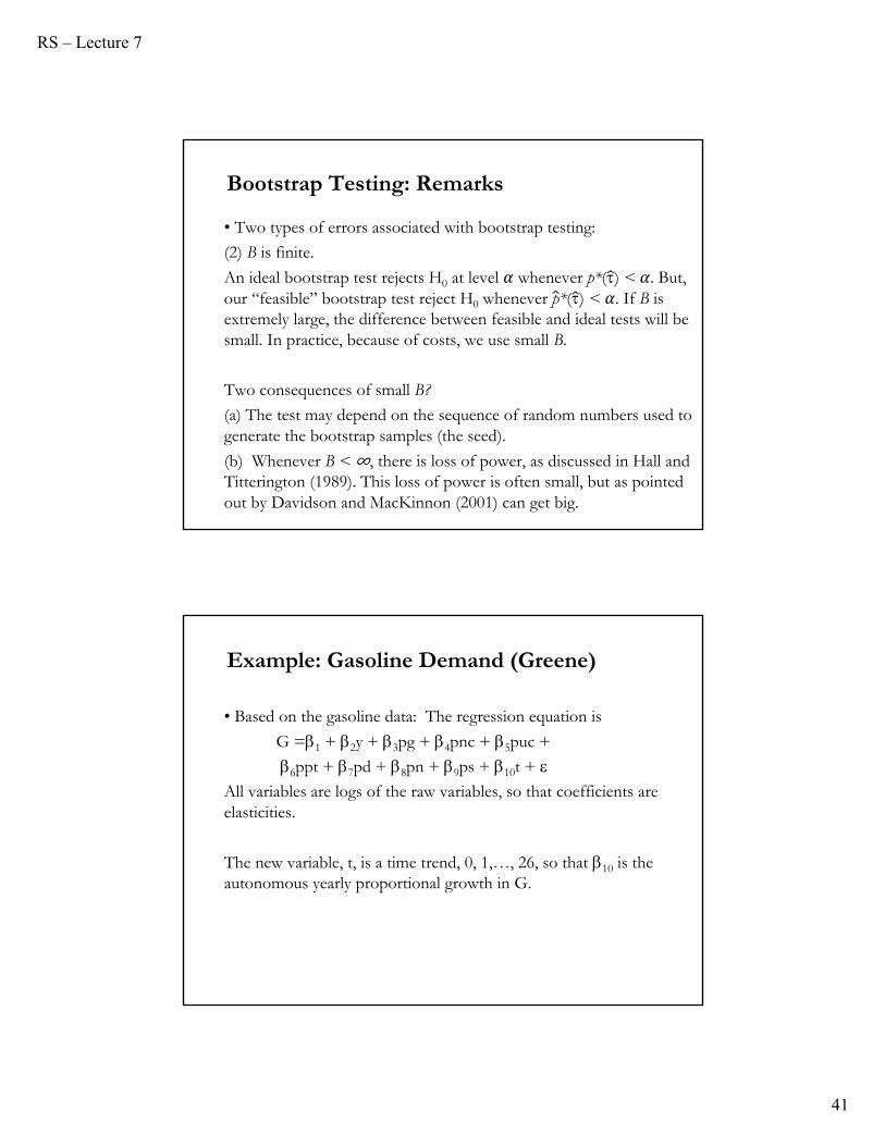
• Two types of errors associated with bootstrap testing:
(2) B is finite.
An ideal bootstrap test rejects H0 at level whenever p*() < . But, our “feasible” bootstrap test reject H0 whenever p*() < . If B is extremely large, the difference between feasible and ideal tests will be small. In practice, because of costs, we use small B.
Two consequences of small B?
(a) The test may depend on the sequence of random numbers used to generate the bootstrap samples (the seed).
(b) Whenever B < ∞, there is loss of power, as discussed in Hall and Titterington (1989). This loss of power is often small, but as pointed out by Davidson and MacKinnon (2001) can get big.
Bootstrap Testing: Remarks
Example: Gasoline Demand (Greene)
• Based on the gasoline data: The regression equation is
G =1 + 2y + 3pg + 4pnc + 5puc +
6ppt + 7pd + 8pn + 9ps + 10t + All variables are logs of the raw variables, so that coefficients are elasticities.
The new variable, t, is a time trend, 0, 1,…, 26, so that 10 is the autonomous yearly proportional growth in G.
RS – Lecture 7
42
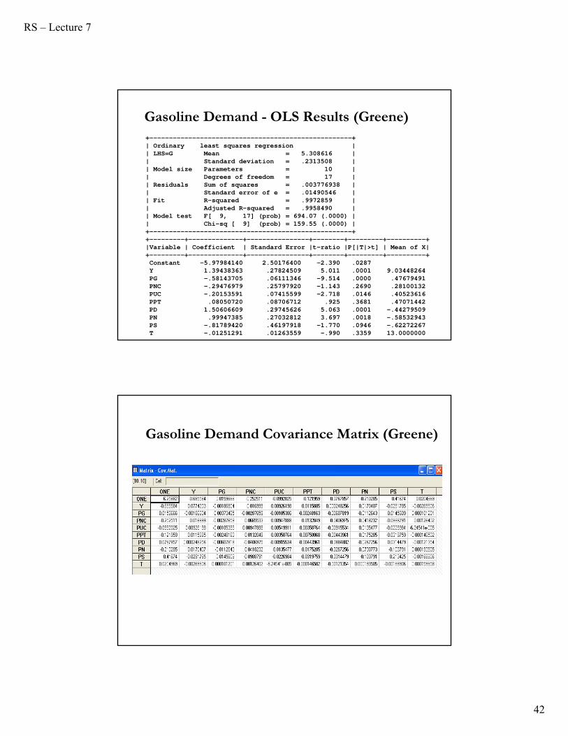
Gasoline Demand - OLS Results (Greene)+----------------------------------------------------+| Ordinary least squares regression || LHS=G Mean = 5.308616 || Standard deviation = .2313508 || Model size Parameters = 10 || Degrees of freedom = 17 || Residuals Sum of squares = .003776938 | | Standard error of e = .01490546 || Fit R-squared = .9972859 || Adjusted R-squared = .9958490 || Model test F[ 9, 17] (prob) = 694.07 (.0000) || Chi-sq [ 9] (prob) = 159.55 (.0000) |+----------------------------------------------------++---------+--------------+----------------+--------+---------+----------+|Variable | Coefficient | Standard Error |t-ratio |P[|T|>t] | Mean of X|+---------+--------------+----------------+--------+---------+----------+Constant -5.97984140 2.50176400 -2.390 .0287Y 1.39438363 .27824509 5.011 .0001 9.03448264PG -.58143705 .06111346 -9.514 .0000 .47679491PNC -.29476979 .25797920 -1.143 .2690 .28100132PUC -.20153591 .07415599 -2.718 .0146 .40523616PPT .08050720 .08706712 .925 .3681 .47071442PD 1.50606609 .29745626 5.063 .0001 -.44279509PN .99947385 .27032812 3.697 .0018 -.58532943PS -.81789420 .46197918 -1.770 .0946 -.62272267T -.01251291 .01263559 -.990 .3359 13.0000000
Gasoline Demand Covariance Matrix (Greene)
RS – Lecture 7
43
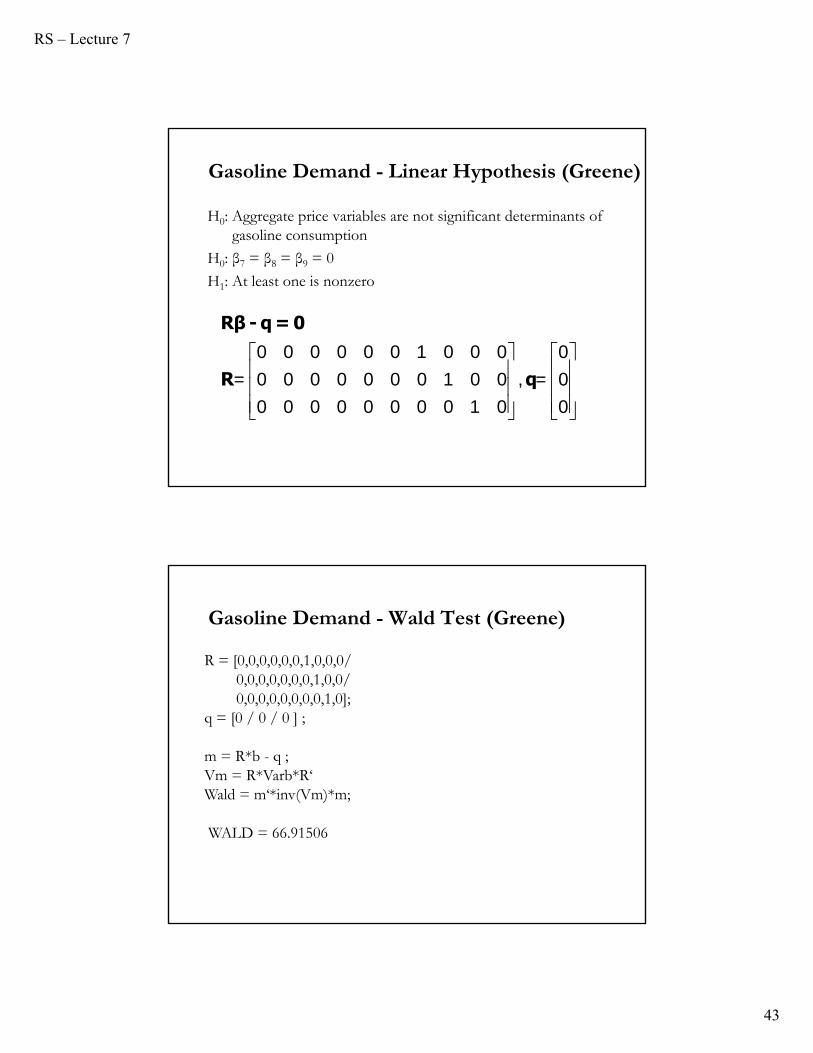
Gasoline Demand - Linear Hypothesis (Greene)
H0: Aggregate price variables are not significant determinants of gasoline consumption
H0: β7 = β8 = β9 = 0
H1: At least one is nonzero
0 0 0 0 0 0 1 0 0 0 0= 0 0 0 0 0 0 0 1 0 0 , = 0
0 0 0 0 0 0 0 0 1 0 0
Rβ - q=0
R q
Gasoline Demand - Wald Test (Greene)
R = [0,0,0,0,0,0,1,0,0,0/0,0,0,0,0,0,0,1,0,0/0,0,0,0,0,0,0,0,1,0];
q = [0 / 0 / 0 ] ;
m = R*b - q ; Vm = R*Varb*R‘Wald = m‘*inv(Vm)*m;
WALD = 66.91506
RS – Lecture 7
44
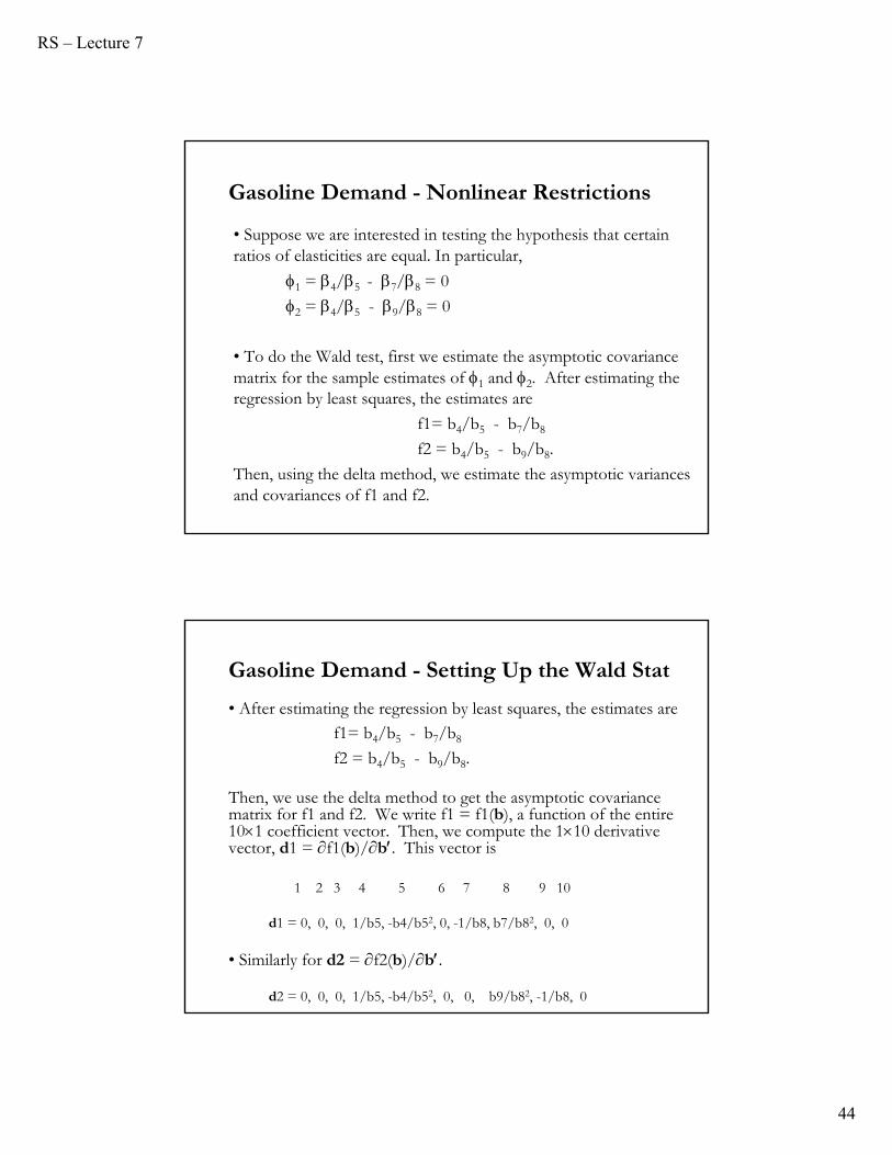
Gasoline Demand - Nonlinear Restrictions
• Suppose we are interested in testing the hypothesis that certain ratios of elasticities are equal. In particular,
1 = 4/5 - 7/8 = 0
2 = 4/5 - 9/8 = 0
• To do the Wald test, first we estimate the asymptotic covariance matrix for the sample estimates of 1 and 2. After estimating the regression by least squares, the estimates are
f1= b4/b5 - b7/b8
f2 = b4/b5 - b9/b8.
Then, using the delta method, we estimate the asymptotic variances and covariances of f1 and f2.
Gasoline Demand - Setting Up the Wald Stat
• After estimating the regression by least squares, the estimates are f1= b4/b5 - b7/b8
f2 = b4/b5 - b9/b8.
Then, we use the delta method to get the asymptotic covariance matrix for f1 and f2. We write f1 = f1(b), a function of the entire 101 coefficient vector. Then, we compute the 110 derivative vector, d1 = f1(b)/b. This vector is
1 2 3 4 5 6 7 8 9 10
d1 = 0, 0, 0, 1/b5, -b4/b52, 0, -1/b8, b7/b82, 0, 0
• Similarly for d2 = f2(b)/b.
d2 = 0, 0, 0, 1/b5, -b4/b52, 0, 0, b9/b82, -1/b8, 0
RS – Lecture 7
45
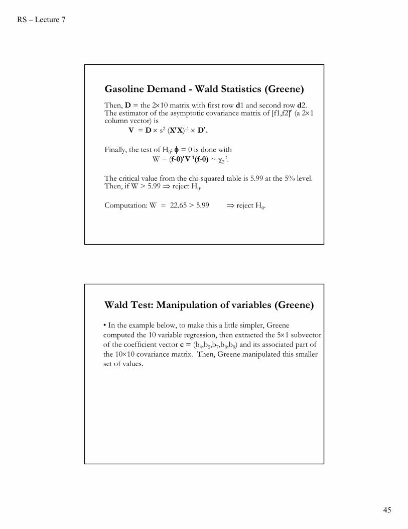
Gasoline Demand - Wald Statistics (Greene)
Then, D = the 210 matrix with first row d1 and second row d2. The estimator of the asymptotic covariance matrix of [f1,f2] (a 21 column vector) is
V = D s2 (XX)-1 D.
Finally, the test of H0: = 0 is done with W = (f-0)V-1(f-0) ~ χ2
2.
The critical value from the chi-squared table is 5.99 at the 5% level. Then, if W > 5.99 reject H0.
Computation: W = 22.65 > 5.99 reject H0.
Wald Test: Manipulation of variables (Greene)
• In the example below, to make this a little simpler, Greene computed the 10 variable regression, then extracted the 51 subvector of the coefficient vector c = (b4,b5,b7,b8,b9) and its associated part of the 1010 covariance matrix. Then, Greene manipulated this smaller set of values.
RS – Lecture 7
46
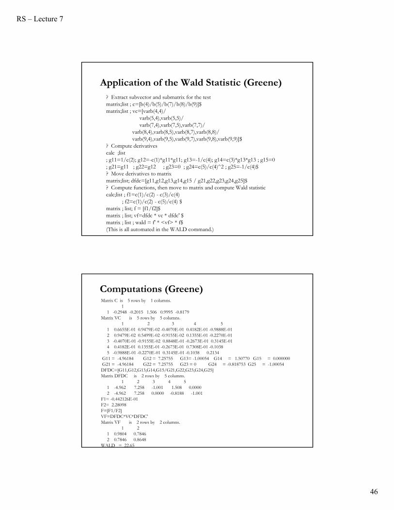
Application of the Wald Statistic (Greene)? Extract subvector and submatrix for the testmatrix;list ; c=[b(4)/b(5)/b(7)/b(8)/b(9)]$matrix;list ; vc=[varb(4,4)/
varb(5,4),varb(5,5)/varb(7,4),varb(7,5),varb(7,7)/
varb(8,4),varb(8,5),varb(8,7),varb(8,8)/varb(9,4),varb(9,5),varb(9,7),varb(9,8),varb(9,9)]$
? Compute derivativescalc ;list ; g11=1/c(2); g12=-c(1)*g11*g11; g13=-1/c(4); g14=c(3)*g13*g13 ; g15=0; g21=g11 ; g22=g12 ; g23=0 ; g24=c(5)/c(4)^2 ; g25=-1/c(4)$? Move derivatives to matrixmatrix;list; dfdc=[g11,g12,g13,g14,g15 / g21,g22,g23,g24,g25]$? Compute functions, then move to matrix and compute Wald statisticcalc;list ; f1=c(1)/c(2) - c(3)/c(4)
; f2=c(1)/c(2) - c(5)/c(4) $matrix ; list; f = [f1/f2]$matrix ; list; vf=dfdc * vc * dfdc' $matrix ; list ; wald = f' * <vf> * f$(This is all automated in the WALD command.)
Computations (Greene)Matrix C is 5 rows by 1 columns.
11 -0.2948 -0.2015 1.506 0.9995 -0.8179
Matrix VC is 5 rows by 5 columns.1 2 3 4 5
1 0.6655E-01 0.9479E-02 -0.4070E-01 0.4182E-01 -0.9888E-012 0.9479E-02 0.5499E-02 -0.9155E-02 0.1355E-01 -0.2270E-013 -0.4070E-01 -0.9155E-02 0.8848E-01 -0.2673E-01 0.3145E-014 0.4182E-01 0.1355E-01 -0.2673E-01 0.7308E-01 -0.10385 -0.9888E-01 -0.2270E-01 0.3145E-01 -0.1038 0.2134
G11 = -4.96184 G12 = 7.25755 G13= -1.00054 G14 = 1.50770 G15 = 0.000000G21 = -4.96184 G22 = 7.25755 G23 = 0 G24 = -0.818753 G25 = -1.00054DFDC=[G11,G12,G13,G14,G15/G21,G22,G23,G24,G25]Matrix DFDC is 2 rows by 5 columns.
1 2 3 4 51 -4.962 7.258 -1.001 1.508 0.00002 -4.962 7.258 0.0000 -0.8188 -1.001
F1= -0.442126E-01F2= 2.28098F=[F1/F2]VF=DFDC*VC*DFDC'Matrix VF is 2 rows by 2 columns.
1 21 0.9804 0.78462 0.7846 0.8648
WALD = 22.65
RS – Lecture 7
47
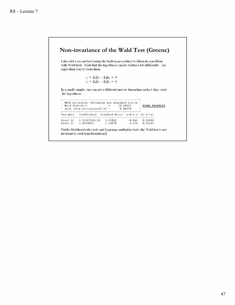
Non-invariance of the Wald Test (Greene)