Kinematics Horizontal and Vertical Equations in one dimension.
Kinematics of Wheeled Robots
1

2
https://www.youtube.com/watch?v=giS41utjlbU
Wheeled Mobile Robots
3
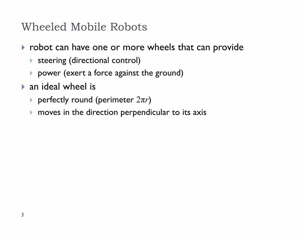
robot can have one or more wheels that can provide steering (directional control) power (exert a force against the ground)
an ideal wheel is perfectly round (perimeter 2πr) moves in the direction perpendicular to its axis
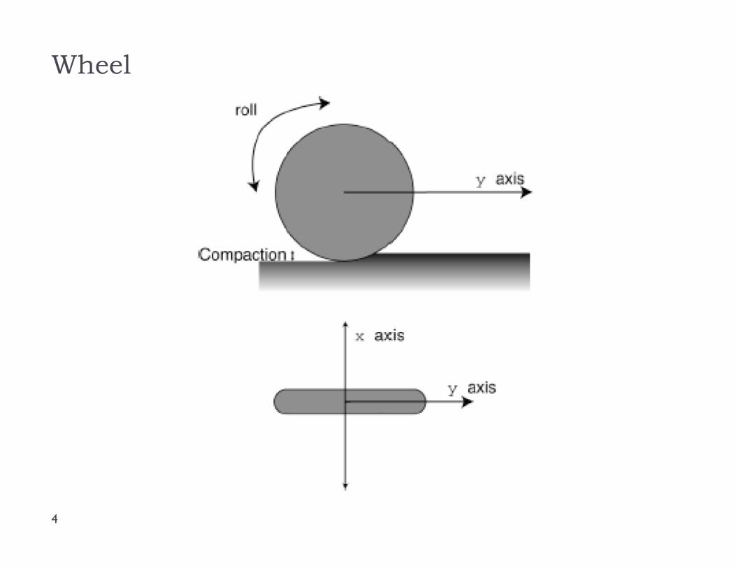
Wheel
4
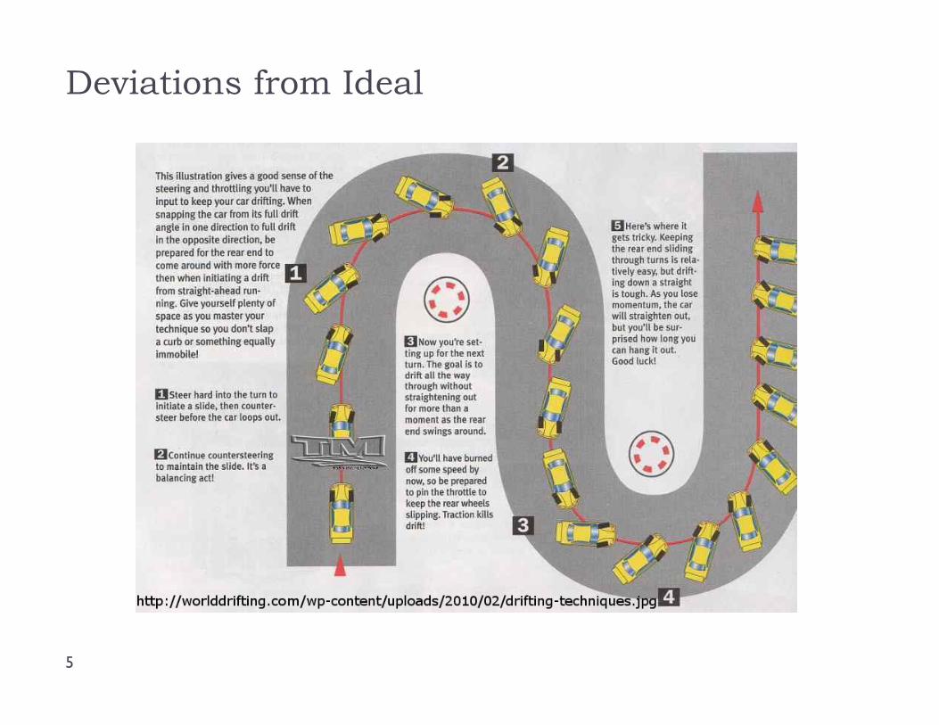
Deviations from Ideal
5
Instantaneous Center of Curvature
6
for smooth rolling motion, all wheels in ground contact must follow a circular path about a common axis of revolution
each wheel must be pointing in its correct direction
revolve with an angular velocity consistent with the motion of the robot each wheel must revolve at its correct speed
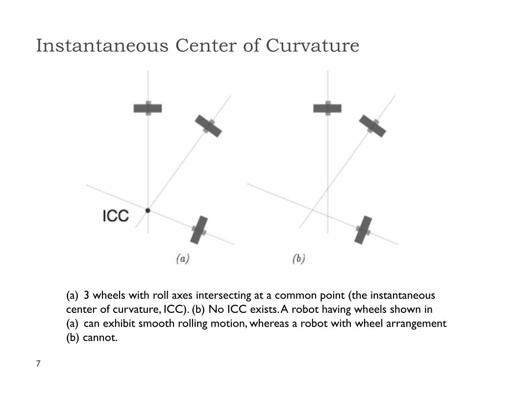
Instantaneous Center of Curvature
7
(a) 3 wheels with roll axes intersecting at a common point (the instantaneouscenter of curvature, ICC). (b) No ICC exists. A robot having wheels shown in(a) can exhibit smooth rolling motion, whereas a robot with wheel arrangement(b) cannot.
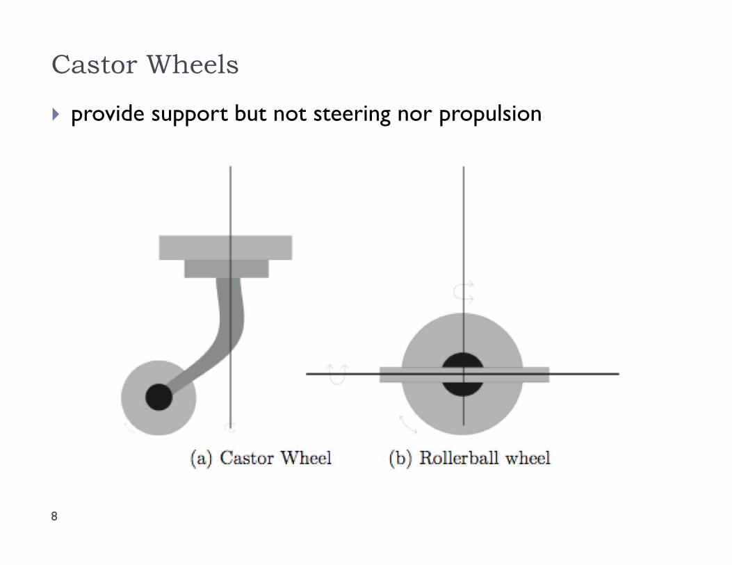
Castor Wheels
8
provide support but not steering nor propulsion
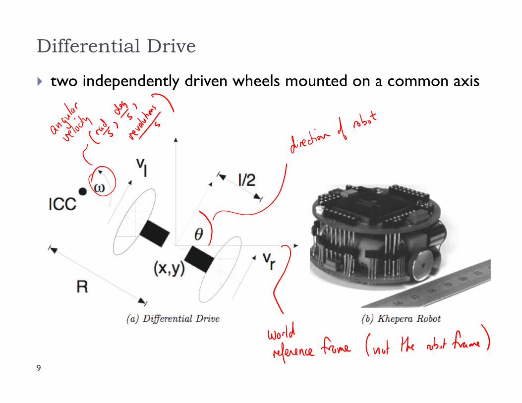
two independently driven wheels mounted on a common axis
Differential Drive
9
Differential Drive
10
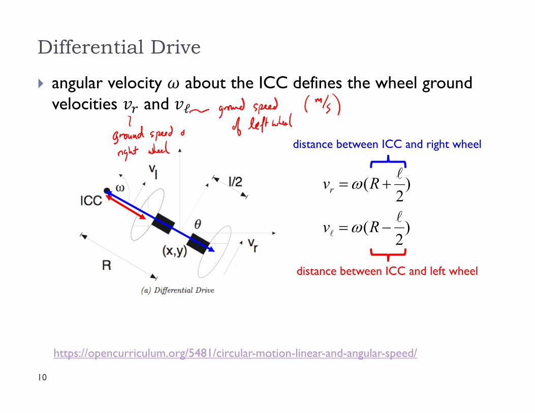
angular velocity about the ICC defines the wheel ground velocities and ℓ
)2
(
)2
(
Rv
Rvr
https://opencurriculum.org/5481/circular-motion-linear-and-angular-speed/
distance between ICC and right wheel
distance between ICC and left wheel
Differential Drive
11
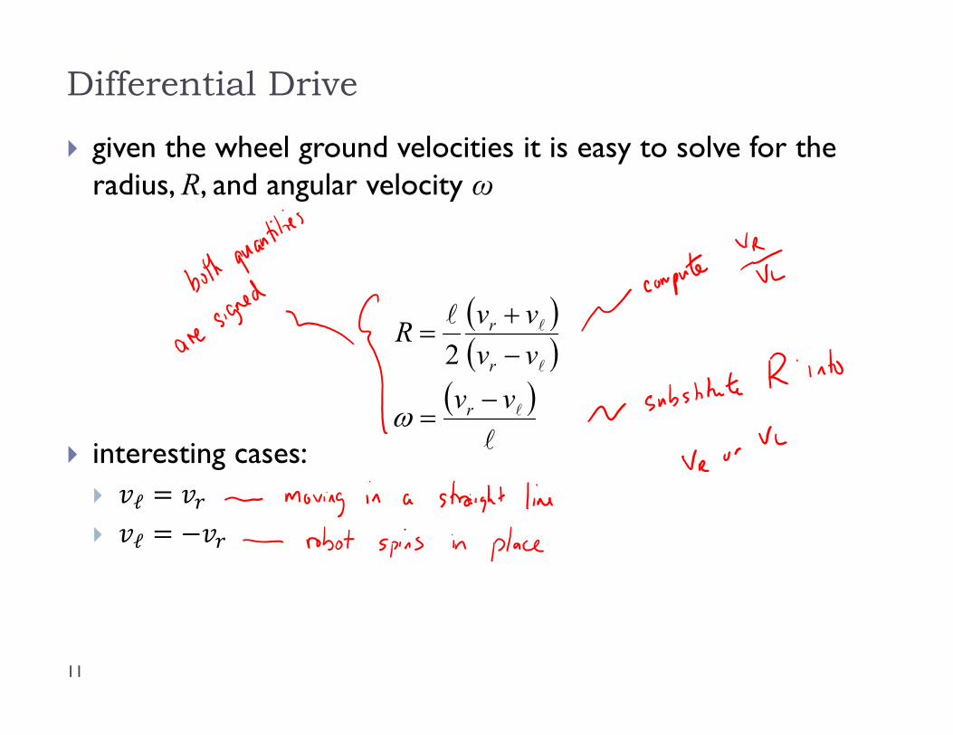
given the wheel ground velocities it is easy to solve for the radius, R, and angular velocity ω
interesting cases: ℓ ℓ
vvvvvvR
r
r
r
2
Tracked Vehicles
12
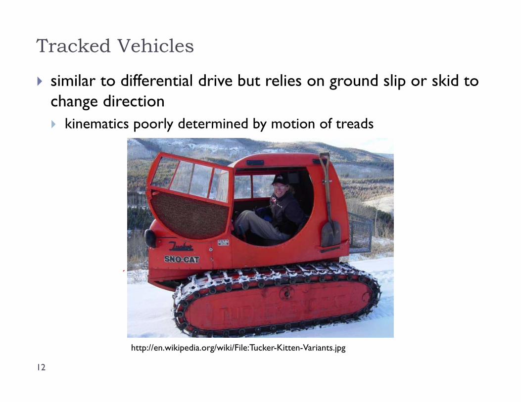
similar to differential drive but relies on ground slip or skid to change direction kinematics poorly determined by motion of treads
http://en.wikipedia.org/wiki/File:Tucker-Kitten-Variants.jpg
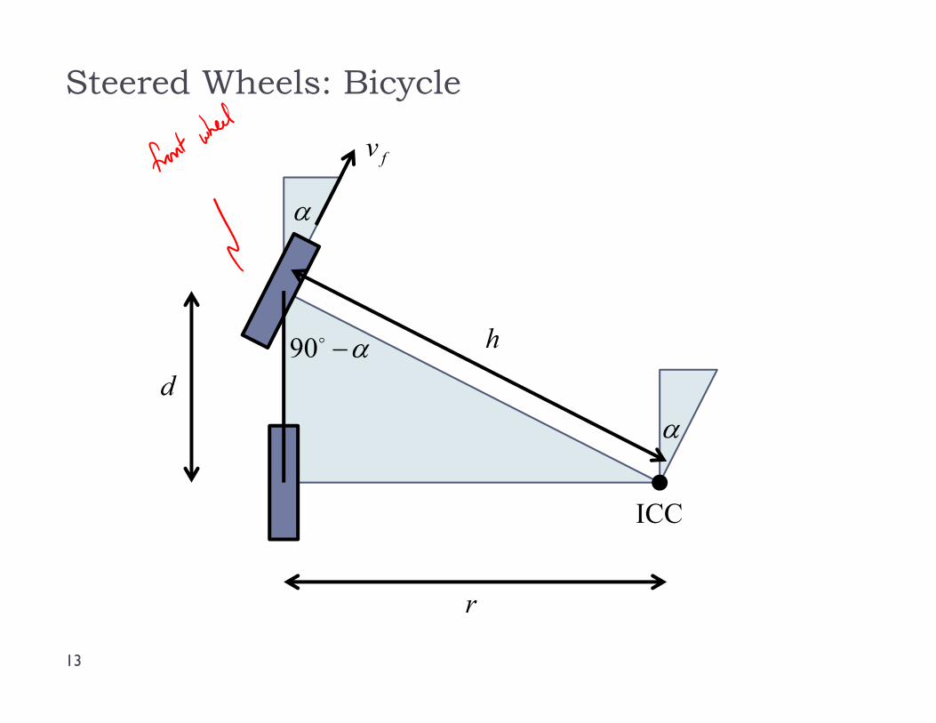
Steered Wheels: Bicycle
13
d
r
h
90
ICC
fv
Steered Wheels: Bicycle
14
important to remember the assumptions in the kinematic model smooth rolling motion in the plane
does not capture all possible motions http://www.youtube.com/watch?v=Cj6ho1-G6tw&NR=1#t=0m25s
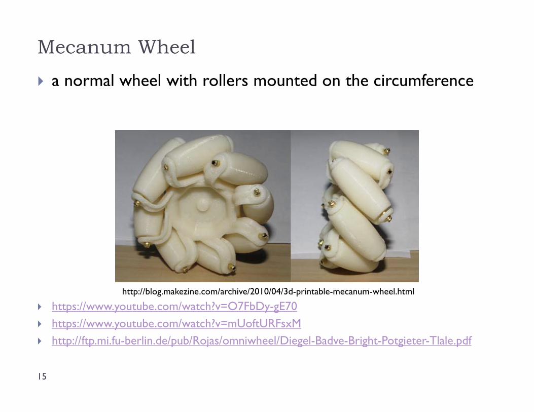
Mecanum Wheel
15
a normal wheel with rollers mounted on the circumference
https://www.youtube.com/watch?v=O7FbDy-gE70 https://www.youtube.com/watch?v=mUoftURFsxM http://ftp.mi.fu-berlin.de/pub/Rojas/omniwheel/Diegel-Badve-Bright-Potgieter-Tlale.pdf
http://blog.makezine.com/archive/2010/04/3d-printable-mecanum-wheel.html
Mecanum Wheel
16
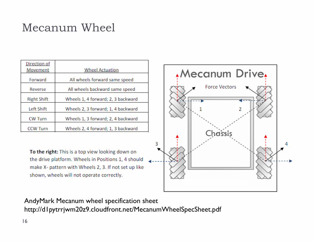
AndyMark Mecanum wheel specification sheethttp://d1pytrrjwm20z9.cloudfront.net/MecanumWheelSpecSheet.pdf
Forward Kinematics
17
serial manipulators given the joint variables, find the pose of the end-effector
mobile robot given the control variables as a function of time, find the pose of the
robot for the differential drive the control variables are often taken to be the
ground velocities of the left and right wheels it is important to note that the wheel velocities are needed as functions of time; a
differential drive that moves forward and then turns right ends up in a very different position than one that turns right then moves forward!
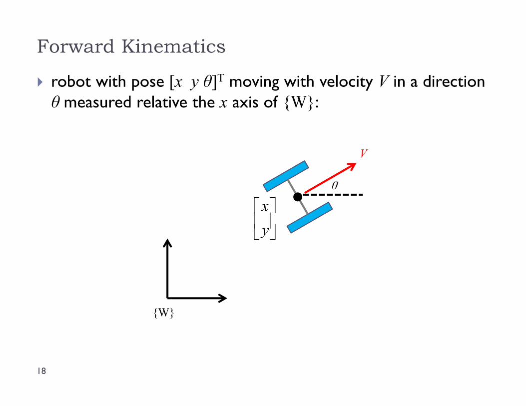
robot with pose [x y θ]T moving with velocity V in a direction θ measured relative the x axis of {W}:
Forward Kinematics
18
V
θ
{W}
yx
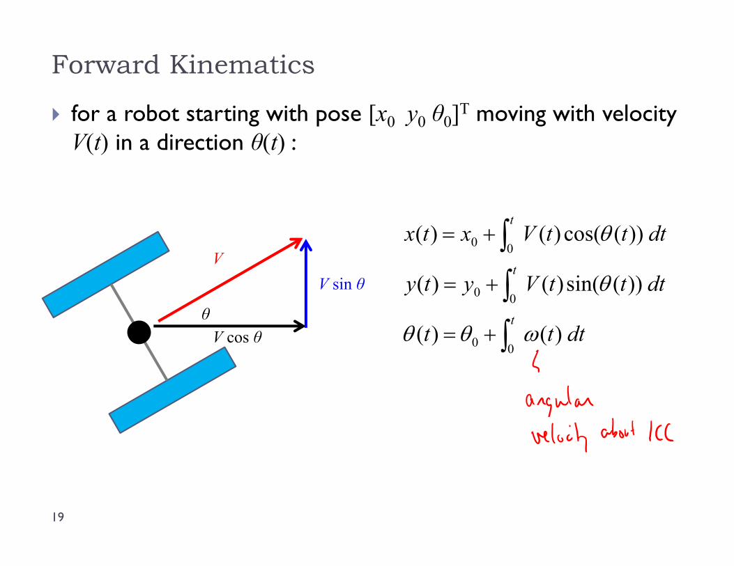
for a robot starting with pose [x0 y0 θ0]T moving with velocity V(t) in a direction θ(t) :
Forward Kinematics
19
t
t
t
dttt
dtttVyty
dtttVxtx
00
00
00
)()(
))(sin()()(
))(cos()()(
V
θV cos θ
V sin θ
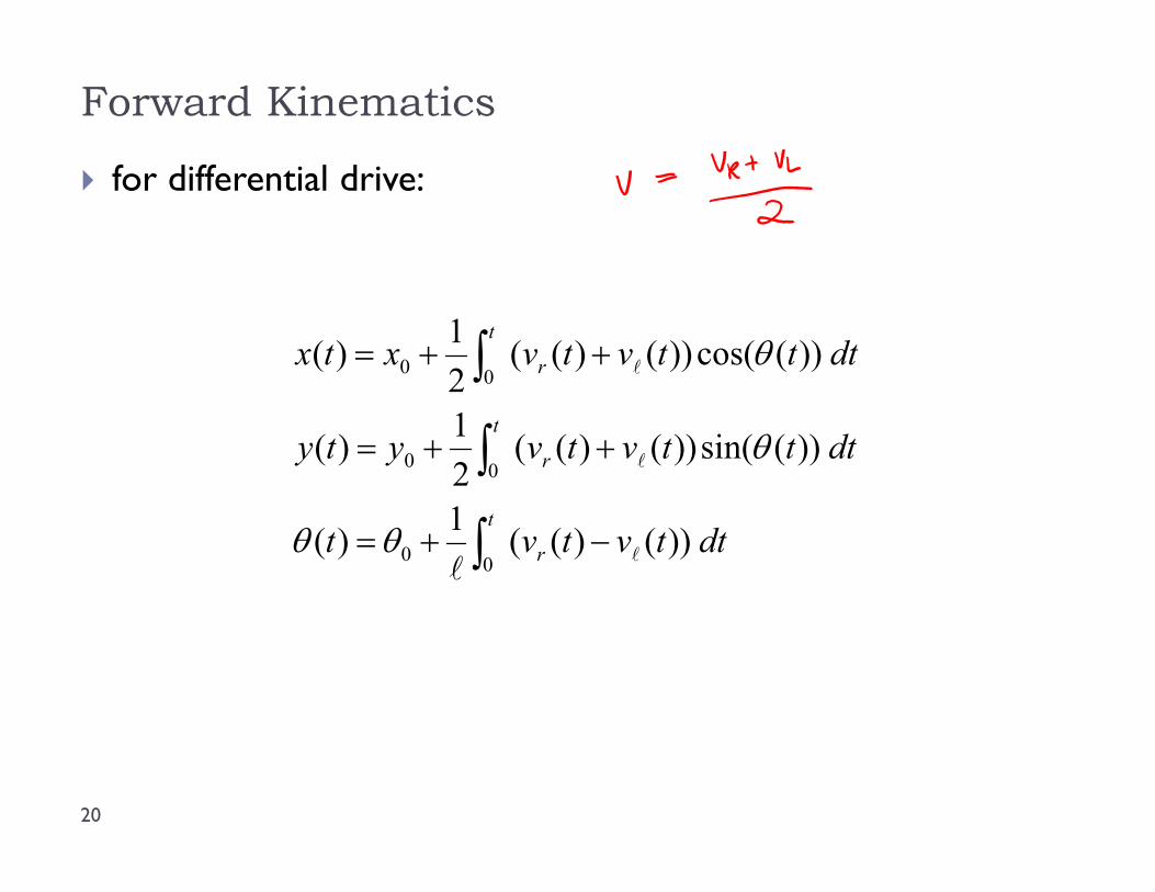
for differential drive:
Forward Kinematics
20
t
r
t
r
t
r
dttvtvt
dtttvtvyty
dtttvtvxtx
00
00
00
))()((1)(
))(sin())()((21)(
))(cos())()((21)(
Sensitivity to Wheel Velocity
21
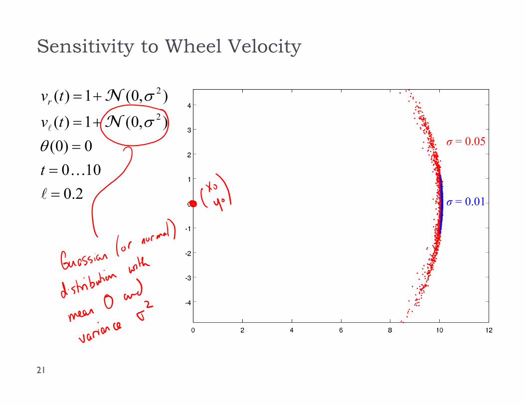
2.01000)0(
),0(1)(
),0(1)(2
2
t
tv
tvr
N
N
σ = 0.05
σ = 0.01
Sensitivity to Wheel Velocity
22
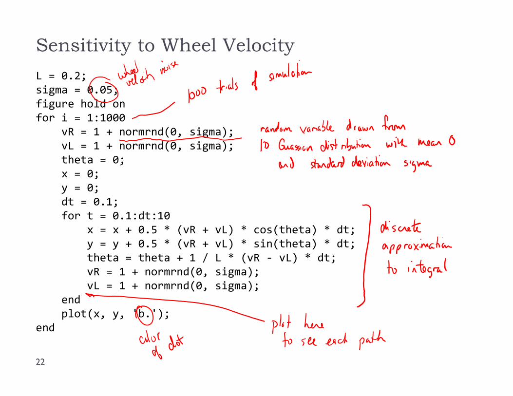
L = 0.2;sigma = 0.05;figure hold onfor i = 1:1000
vR = 1 + normrnd(0, sigma);vL = 1 + normrnd(0, sigma);theta = 0;x = 0;y = 0;dt = 0.1;for t = 0.1:dt:10
x = x + 0.5 * (vR + vL) * cos(theta) * dt;y = y + 0.5 * (vR + vL) * sin(theta) * dt;theta = theta + 1 / L * (vR ‐ vL) * dt;vR = 1 + normrnd(0, sigma);vL = 1 + normrnd(0, sigma);
endplot(x, y, 'b.');
end
Mobile Robot Forward Kinematics
23
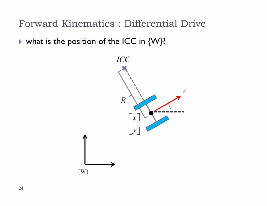
what is the position of the ICC in {W}?
Forward Kinematics : Differential Drive
24
V
θ
{W}
yx
R
ICC
Forward Kinematics : Differential Drive
25
V
θ
{W}
yx
R
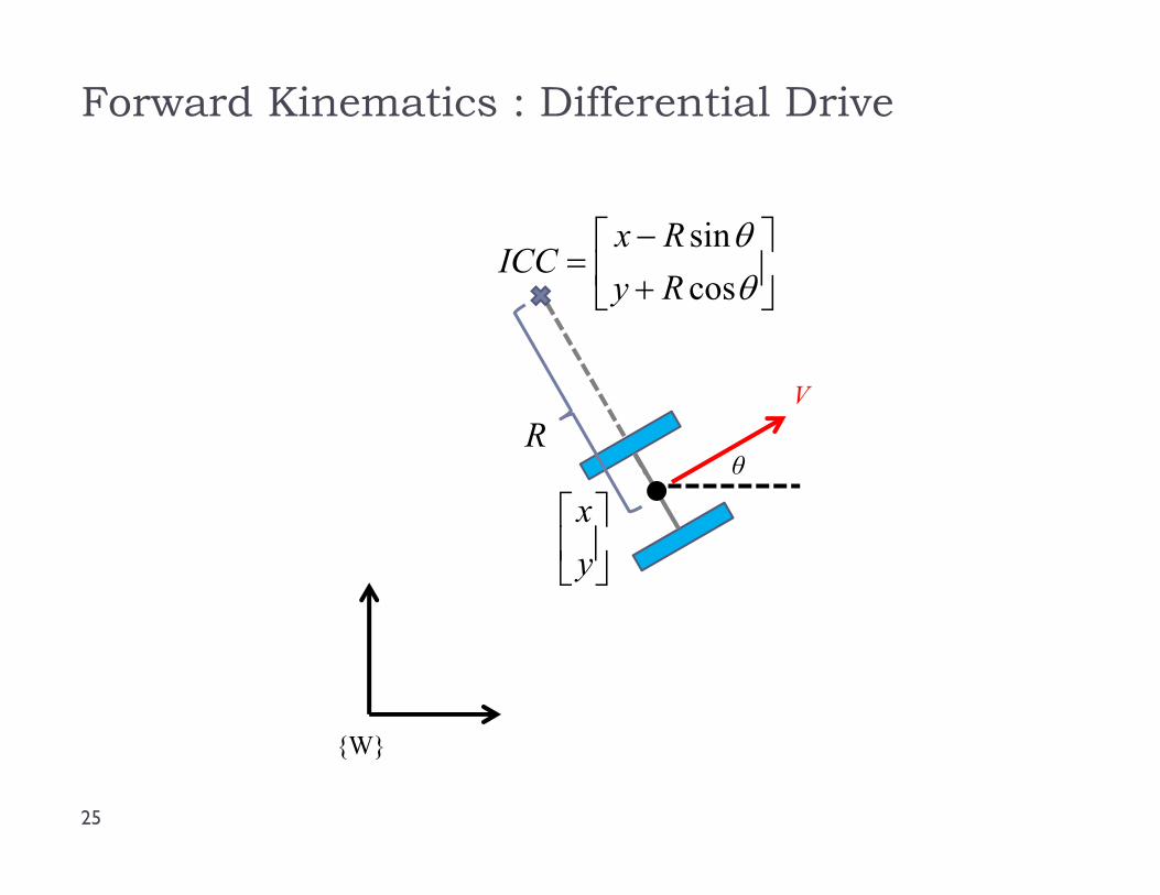
cossinRyRx
ICC
Forward Kinematics : Differential Drive
26
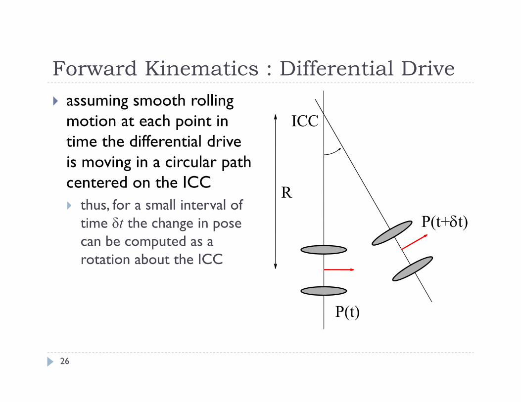
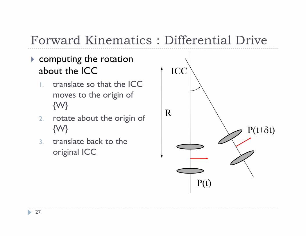
assuming smooth rolling motion at each point in time the differential drive is moving in a circular path centered on the ICC thus, for a small interval of
time δt the change in pose can be computed as a rotation about the ICC
ICC
R
P(t)
P(t+t)
Forward Kinematics : Differential Drive
27
computing the rotation about the ICC1. translate so that the ICC
moves to the origin of {W}
2. rotate about the origin of {W}
3. translate back to the original ICC
ICC
R
P(t)
P(t+t)
Forward Kinematics : Differential Drive
28
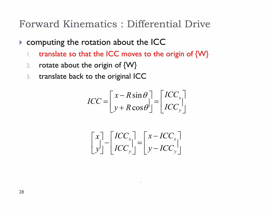
computing the rotation about the ICC1. translate so that the ICC moves to the origin of {W}2. rotate about the origin of {W}3. translate back to the original ICC
y
x
ICCICC
RyRx
ICC
cossin
y
x
y
x
ICCyICCx
ICCICC
yx
Forward Kinematics : Differential Drive
29
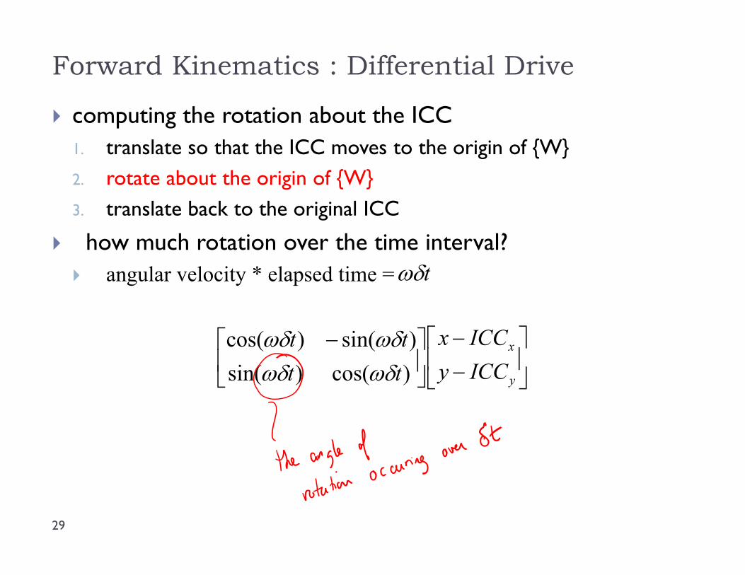
computing the rotation about the ICC1. translate so that the ICC moves to the origin of {W}2. rotate about the origin of {W}3. translate back to the original ICC
how much rotation over the time interval? angular velocity * elapsed time =
y
x
ICCyICCx
tttt)cos()sin()sin()cos(
t
Forward Kinematics : Differential Drive
30
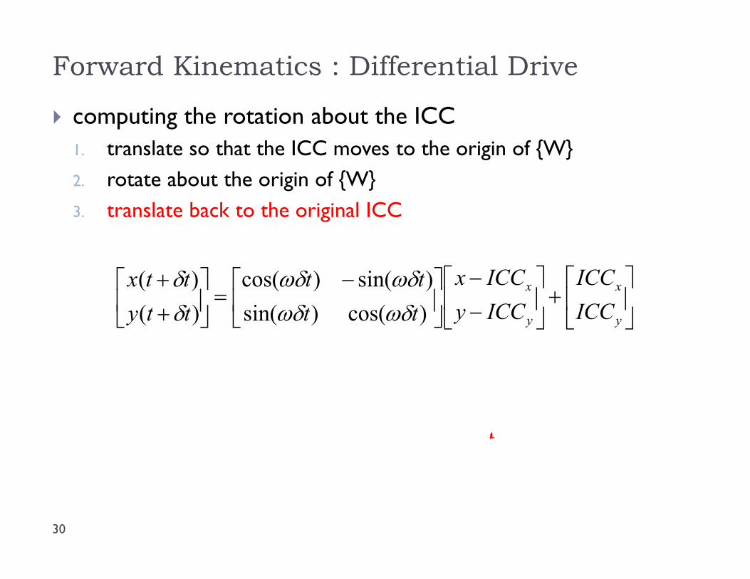
computing the rotation about the ICC1. translate so that the ICC moves to the origin of {W}2. rotate about the origin of {W}3. translate back to the original ICC
y
x
y
x
ICCICC
ICCyICCx
tttt
ttyttx
)cos()sin()sin()cos(
)()(
Forward Kinematics : Differential Drive
31
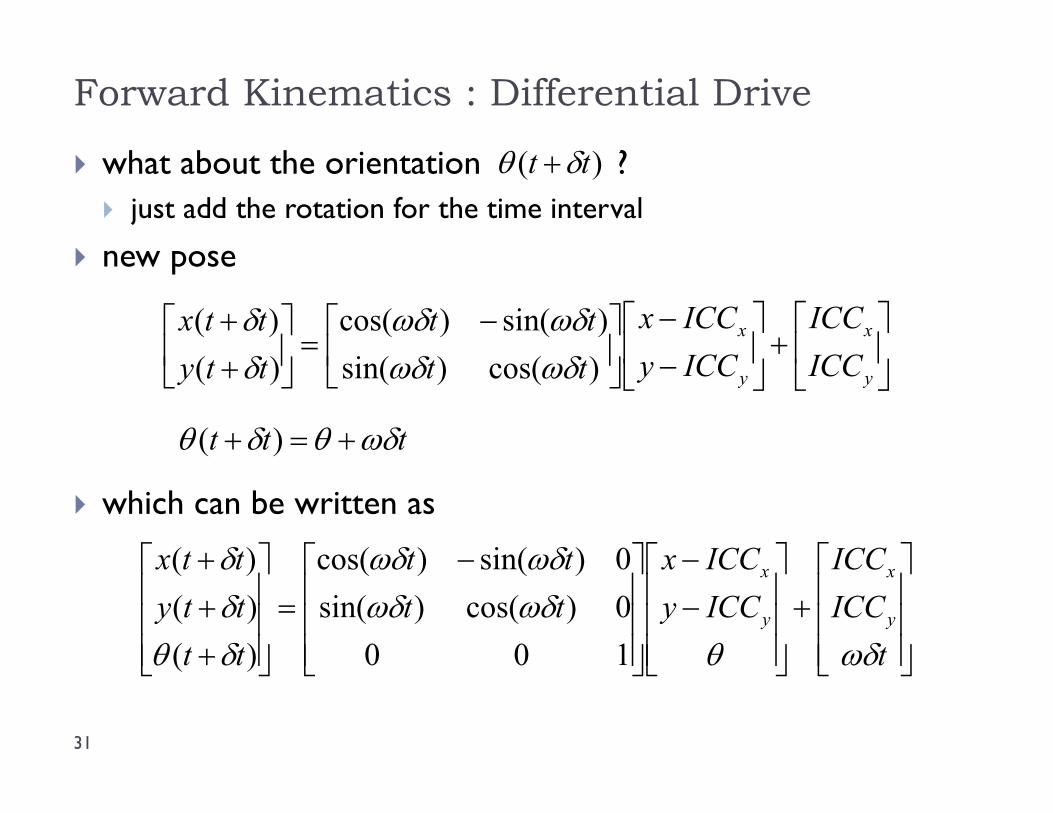
what about the orientation ? just add the rotation for the time interval
new pose
which can be written as
)( tt
y
x
y
x
ICCICC
ICCyICCx
tttt
ttyttx
)cos()sin()sin()cos(
)()(
ttt )(
tICCICC
ICCyICCx
tttt
ttttyttx
y
x
y
x
1000)cos()sin(0)sin()cos(
)()()(
Forward Kinematics: Differential Drive
32
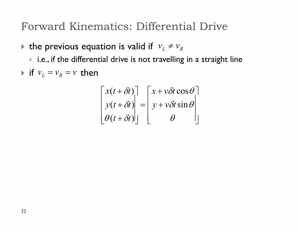
the previous equation is valid if i.e., if the differential drive is not travelling in a straight line
if then
RL vv
vvv RL
sincos
)()()(
tvytvx
ttttyttx
Sensitivity to Wheel Velocity
33
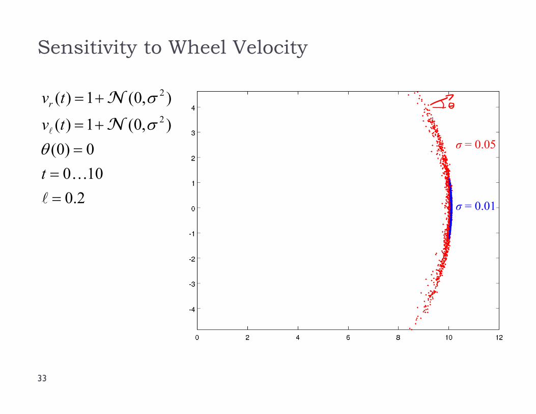
2.01000)0(
),0(1)(
),0(1)(2
2
t
tv
tvr
N
N
σ = 0.05
σ = 0.01
Sensitivity to Wheel Velocity
34
given the forward kinematics of the differential drive it is easy to write a simulation of the motion we need a way to draw random numbers from a normal distribution in Matlab
randn(n) returns an n-by-n matrix containing pseudorandom values drawn from the standard normal distribution
see mvnrnd for random values from a multivariate normal distribution
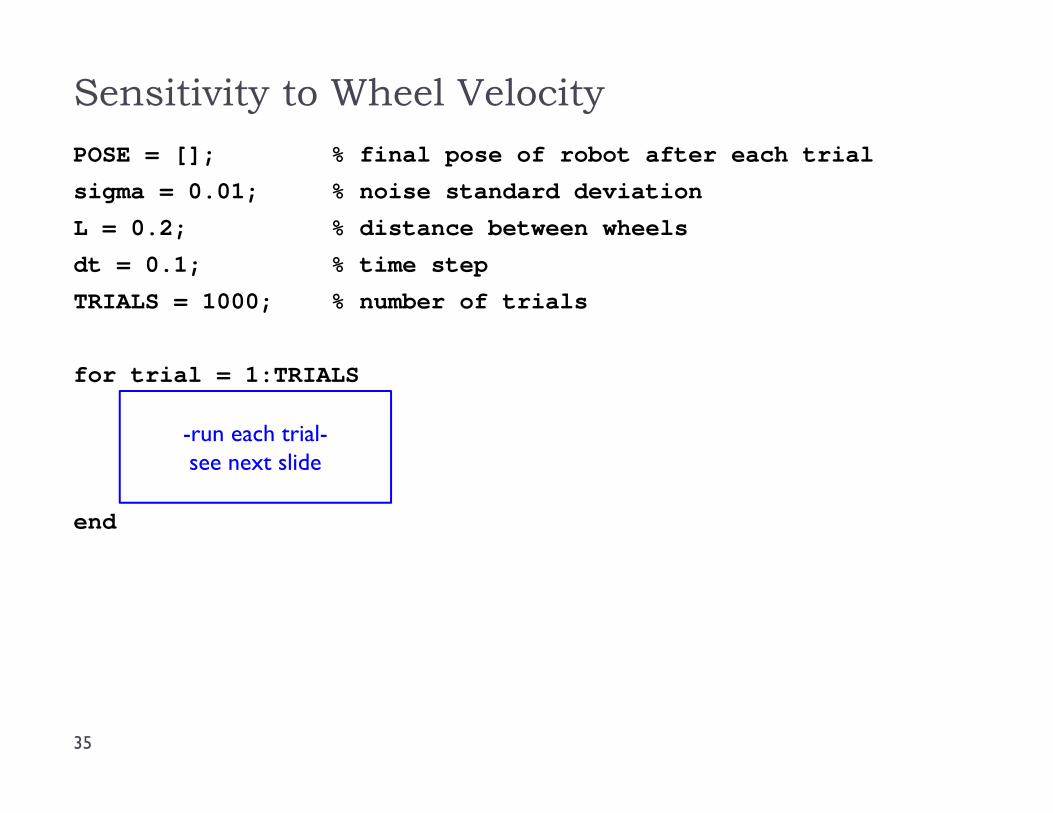
Sensitivity to Wheel Velocity
35
POSE = []; % final pose of robot after each trial
sigma = 0.01; % noise standard deviation
L = 0.2; % distance between wheels
dt = 0.1; % time step
TRIALS = 1000; % number of trials
for trial = 1:TRIALS
end
-run each trial-see next slide
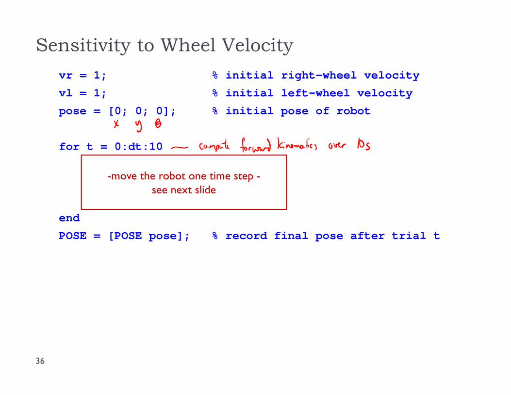
Sensitivity to Wheel Velocity
36
vr = 1; % initial right-wheel velocity
vl = 1; % initial left-wheel velocity
pose = [0; 0; 0]; % initial pose of robot
for t = 0:dt:10
end
POSE = [POSE pose]; % record final pose after trial t
-move the robot one time step -see next slide
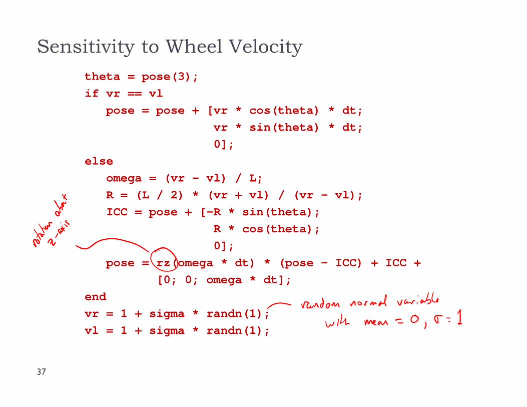
Sensitivity to Wheel Velocity
37
theta = pose(3);if vr == vl
pose = pose + [vr * cos(theta) * dt;vr * sin(theta) * dt;0];
elseomega = (vr – vl) / L;R = (L / 2) * (vr + vl) / (vr – vl);ICC = pose + [-R * sin(theta);
R * cos(theta);0];
pose = rz(omega * dt) * (pose – ICC) + ICC +[0; 0; omega * dt];
endvr = 1 + sigma * randn(1);vl = 1 + sigma * randn(1);