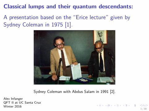
Classical lumps and their quantum descendants:

A presentation based on the “Erice lecture” given bySydney Coleman in 1975 [1].

Sydney Coleman with Abdus Salam in 1991 [2].Alex InfangerQFT II at UC Santa CruzWinter 2016

1 / 30

Let Θ00(x, t) be the energy density of a classical field theory. Wecall a solution φ of the equation of motion (EOM) dissipative if

limt→∞

maxx

Θ00(x, t) = 0.

Not all theories need be like this! There exist theories withnon-dissipative behavior and these include some spontaneouslybroken gauge theories.

2 / 30

A simple example

Consider one spatial dimension and ignore derivative interactions

L = 12∂µφ∂

µφ− U(φ).

The energy of any field configuration is given by

E =∫

dx(1

2 (∂0φ)2 + 12 (∂1φ)2 + U(φ)

).

3 / 30

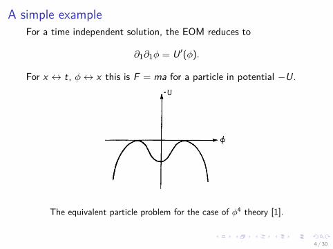
A simple exampleFor a time independent solution, the EOM reduces to

∂1∂1φ = U ′(φ).

For x ↔ t, φ↔ x this is F = ma for a particle in potential −U.

The equivalent particle problem for the case of φ4 theory [1].

4 / 30

A simple example

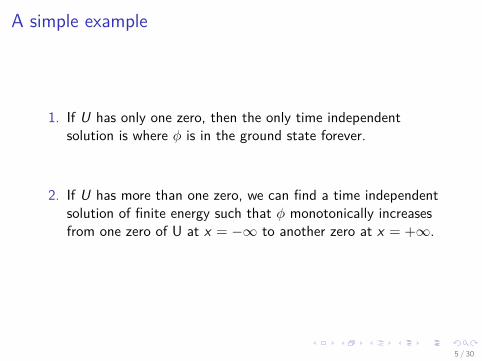
1. If U has only one zero, then the only time independentsolution is where φ is in the ground state forever.

2. If U has more than one zero, we can find a time independentsolution of finite energy such that φ monotonically increasesfrom one zero of U at x = −∞ to another zero at x = +∞.

5 / 30

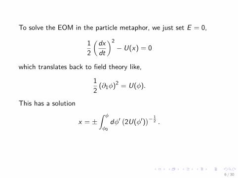
To solve the EOM in the particle metaphor, we just set E = 0,

12

(dxdt

)2− U(x) = 0

which translates back to field theory like,

12 (∂1φ)2 = U(φ).

This has a solution

x = ±∫ φ

φ0dφ′

(2U(φ′)

)− 12 .

6 / 30

Are the solutions stable?

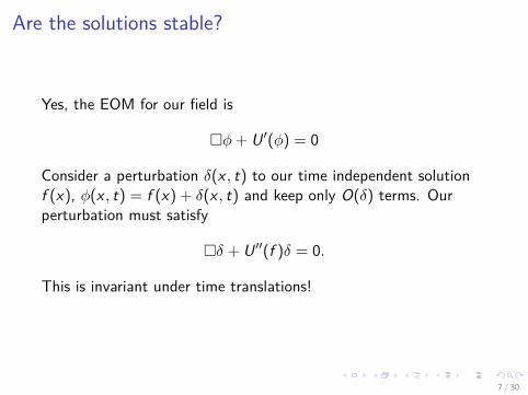
Yes, the EOM for our field is

�φ+ U ′(φ) = 0

Consider a perturbation δ(x , t) to our time independent solutionf (x), φ(x , t) = f (x) + δ(x , t) and keep only O(δ) terms. Ourperturbation must satisfy

�δ + U ′′(f )δ = 0.

This is invariant under time translations!

7 / 30

Are the solutions stable?

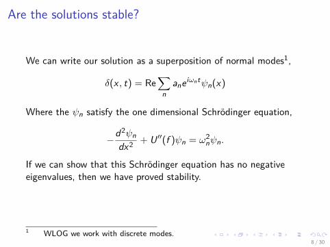
We can write our solution as a superposition of normal modes1,

δ(x , t) = Re∑

naneiωntψn(x)

Where the ψn satisfy the one dimensional Schrodinger equation,

−d2ψndx2 + U ′′(f )ψn = ω2

nψn.

If we can show that this Schrodinger equation has no negativeeigenvalues, then we have proved stability.

1 WLOG we work with discrete modes.8 / 30

Are the solutions stable?

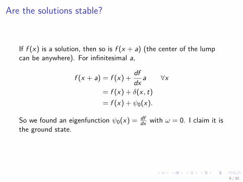
If f (x) is a solution, then so is f (x + a) (the center of the lumpcan be anywhere). For infinitesimal a,

f (x + a) = f (x) + dfdx a ∀x

= f (x) + δ(x , t)= f (x) + ψ0(x).

So we found an eigenfunction ψ0(x) = dfdx with ω = 0. I claim it is

the ground state.

9 / 30

Are the solutions stable?

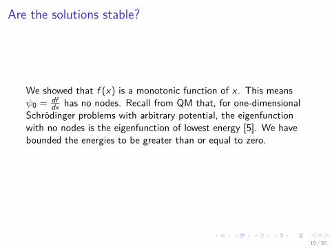
We showed that f (x) is a monotonic function of x . This meansψ0 = df

dx has no nodes. Recall from QM that, for one-dimensionalSchrodinger problems with arbitrary potential, the eigenfunctionwith no nodes is the eigenfunction of lowest energy [5]. We havebounded the energies to be greater than or equal to zero.

10 / 30

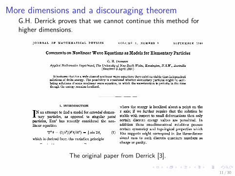
More dimensions and a discouraging theoremG.H. Derrick proves that we cannot continue this method forhigher dimensions.

The original paper from Derrick [3].

11 / 30

More dimensions and a discouraging theorem

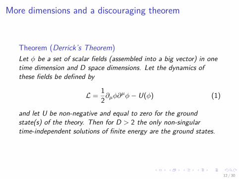
Theorem (Derrick’s Theorem)Let φ be a set of scalar fields (assembled into a big vector) in onetime dimension and D space dimensions. Let the dynamics ofthese fields be defined by

L = 12∂µφ∂

µφ− U(φ) (1)

and let U be non-negative and equal to zero for the groundstate(s) of the theory. Then for D > 2 the only non-singulartime-independent solutions of finite energy are the ground states.

12 / 30

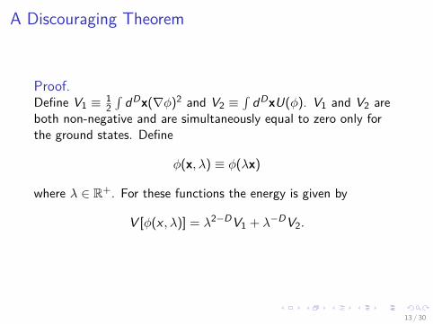
A Discouraging Theorem

Proof.Define V1 ≡ 1

2∫

dDx(∇φ)2 and V2 ≡∫

dDxU(φ). V1 and V2 areboth non-negative and are simultaneously equal to zero only forthe ground states. Define

φ(x, λ) ≡ φ(λx)

where λ ∈ R+. For these functions the energy is given by

V [φ(x , λ)] = λ2−DV1 + λ−DV2.

13 / 30

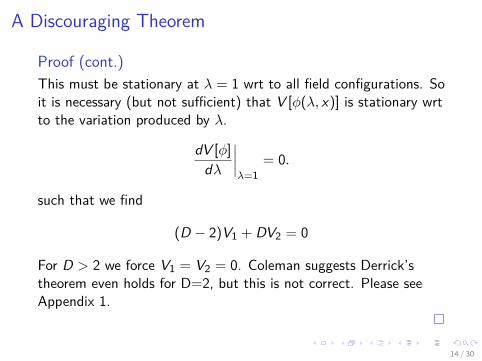
A Discouraging Theorem

Proof (cont.)This must be stationary at λ = 1 wrt to all field configurations. Soit is necessary (but not sufficient) that V [φ(λ, x)] is stationary wrtto the variation produced by λ.

dV [φ]dλ

∣∣∣∣λ=1

= 0.

such that we find

(D − 2)V1 + DV2 = 0

For D > 2 we force V1 = V2 = 0. Coleman suggests Derrick’stheorem even holds for D=2, but this is not correct. Please seeAppendix 1.

14 / 30

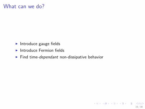
What can we do?

I Introduce gauge fieldsI Introduce Fermion fieldsI Find time-dependant non-dissipative behavior

15 / 30

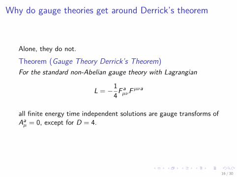
Why do gauge theories get around Derrick’s theorem

Alone, they do not.

Theorem (Gauge Theory Derrick’s Theorem)For the standard non-Abelian gauge theory with Lagrangian

L = −14F a

µνFµνa

all finite energy time independent solutions are gauge transforms ofAaµ = 0, except for D = 4.

16 / 30

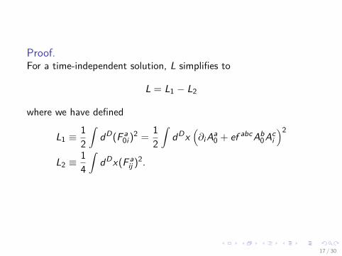
Proof.For a time-independent solution, L simplifies to

L = L1 − L2

where we have defined

L1 ≡12

∫dD(F a

0i )2 = 12

∫dDx

(∂i Aa

0 + ef abcAb0Ac

i

)2

L2 ≡14

∫dDx(F a

ij )2.

17 / 30

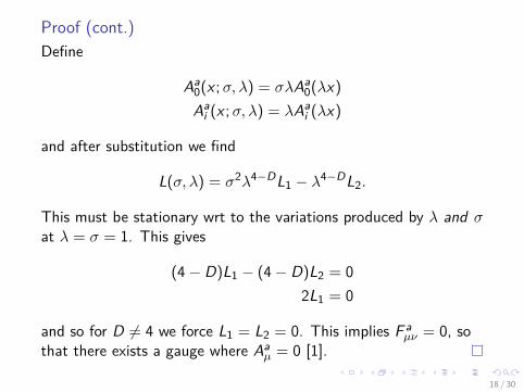
Proof (cont.)Define

Aa0(x ;σ, λ) = σλAa

0(λx)Aa

i (x ;σ, λ) = λAai (λx)

and after substitution we find

L(σ, λ) = σ2λ4−DL1 − λ4−DL2.

This must be stationary wrt to the variations produced by λ and σat λ = σ = 1. This gives

(4− D)L1 − (4− D)L2 = 02L1 = 0

and so for D 6= 4 we force L1 = L2 = 0. This implies F aµν = 0, so

that there exists a gauge where Aaµ = 0 [1].

18 / 30

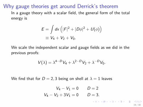
Why gauge theories get around Derrick’s theoremIn a gauge theory with a scalar field, the general form of the totalenergy is

E =∫

dx(|F |2 + |Dφ|2 + U(φ)

)≡ V4 + V2 + V0.

We scale the independent scalar and gauge fields as we did in theprevious proofs:

V (λ) = λ4−DV4 + λ2−DV2 + λ−DV0.

We find that for D = 2, 3 being on shell at λ = 1 leaves

V4 − V1 = 0 D = 2V4 − V2 + 3V1 = 0 D = 3.

19 / 30

Another path

Another way to find non-dissipative behavior in field theories is todiscover & use topological conservation laws.

20 / 30

Another path: Topological Conservation laws

Again, finite energy solutions push the fields to a zero of U atinfinity. That is,

U (φ(±∞, t)) = 0,

and since the zeroes of U form a finite set,

∂0φ(±∞, t) = 0.

If U has multiple zeros, this equation can be used to prove theexistence of non-dissipative solutions!

21 / 30

Another path: Topological Conservation lawsConsider the 1D φ4 theory again, where we shift the minima tooccur at U = 0:

U = λ

2φ4 − µ2φ2 + µ4

2λ.

If we demand the initial condition at one time,

φ(∞, t) = −φ(−∞, t)

we have it for all time. By continuity in x , for all t there existssome x s.t. φ = 0. At this point, Θ00(x , t) ≥ U(0). ButU(0) = µ2

2λ such that for all t

maxx

Θ00(x , t) ≥ µ2

2λ.

And so we have found non-dissipative behavior.

22 / 30

Another path: Topological Conservation laws

What just happened? Recall the conservation law:

∂0φ(±∞, t) = 0.

It did not come from a symmetry in the Lagrangian. Instead, itarose because we had a discrete set of zeros of the potential. Inanother sense, we have divided the space of non-singularfinite-energy solutions at a fixed time into subspaces (labeled byφ(±∞, t)) which are disconnected “in the normal topologicalsense”[1].

23 / 30

“In the normal topological sense”

Definition (Topological Space).A topological space is an ordered pair (X , τ) where X is a set andτ is a collection of subsets of X that satisfy

1. The empty set ∅ and X belong to τ .2. Any (finite or infinite) union of members of τ belong to τ .3. Any finite intersection of members of τ belong to τ .

The members of τ are called open.

Definition (Disconnected).A topological space (X , τ) is said to be disconnected iff a pair ofdisjoint, non-empty open subsets X1, X2 exists, such thatX = X1 ∪ X2.

24 / 30

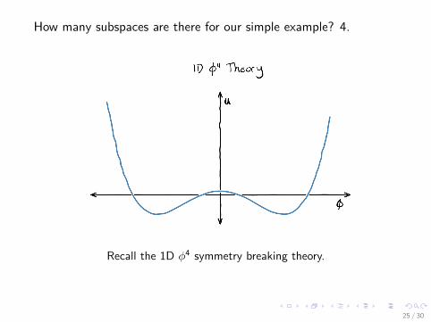
How many subspaces are there for our simple example? 4.

Recall the 1D φ4 symmetry breaking theory.

25 / 30

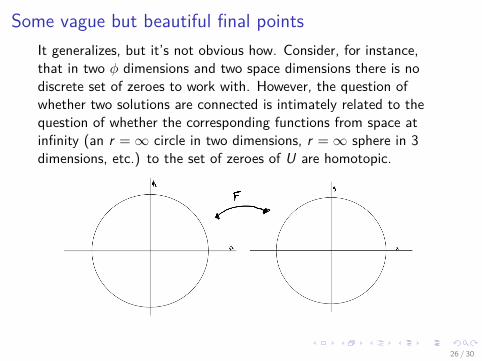
Some vague but beautiful final pointsIt generalizes, but it’s not obvious how. Consider, for instance,that in two φ dimensions and two space dimensions there is nodiscrete set of zeroes to work with. However, the question ofwhether two solutions are connected is intimately related to thequestion of whether the corresponding functions from space atinfinity (an r =∞ circle in two dimensions, r =∞ sphere in 3dimensions, etc.) to the set of zeroes of U are homotopic.

26 / 30

Some vague but beautiful final points

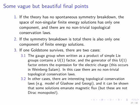
1. If the theory has no spontaneous symmetry breakdown, thespace of non-singular finite energy solutions has only onecomponent, and there are no non-trivial topologicalconservation laws.

2. If the symmetry breakdown is total there is also only onecomponent of finite energy solutions.

3. If one Goldstone survives, there are two cases:3.1 The gauge group when written as a product of simple Lie

groups contains a U(1) factor, and the generator of this U(1)factor enters the expression for the electric charge (this occursin Weinberg-Salam). In this case there are no non-trivialtopological conservation laws.

3.2 In other cases, there are interesting topological conservationlaws (e.g. model of Glashow and Georgi), and it can be shownthat some solutions emanate magnetic flux (but these are notDirac monopoles!).

27 / 30

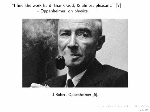
“I find the work hard, thank God, & almost pleasant.” [7]– Oppenheimer, on physics.

J Robert Oppenheimer [6].

28 / 30

References

[1] Coleman, Sidney. Aspects of Symmetry: Selected Erice Lectures. Cambridge: Cambridge University Press,1985. http://ebooks.cambridge.org/ref/id/CBO9780511565045.

[2] http://fr.cdn.v5.futura-sciences.com/sources/images/actu/rte/magic/13642ResImg.php.jpg

[3] Derrick, G. H. “Comments on Nonlinear Wave Equations as Models for Elementary Particles.” Journal ofMathematical Physics 5, no. 9 (September 1, 1964): 1252âĂŞ54. doi:10.1063/1.1704233.

[4] Parenti, C., F. Strocchi, and G. Velo. “Solutions of Classical Field Equations with Locally Finite KineticEnergy.” Physics Letters B 59, no. 2 (October 27, 1975): 157âĂŞ58. doi:10.1016/0370-2693(75)90691-7.

[5] Morse, Philip McCord, Herman Feshbach, and G. P. Harnwell. Methods of Theoretical Physics, Part I.Boston, Mass: McGraw-Hill Book Company, 1953.

[6] AM, Richard Rhodes On 5/15/13 at 4:45. “The Man With the Bomb.” Newsweek, May 15, 2013.http://www.newsweek.com/2013/05/15/why-robert-oppenheimers-atomic-bomb-still-haunts-us-237382.html.

[7] Bird, Kai, and Martin J. Sherwin. American Prometheus: the triumph and tragedy of J. RobertOppenheimer. Alfred a Knopf Incorporated, 2005.

29 / 30

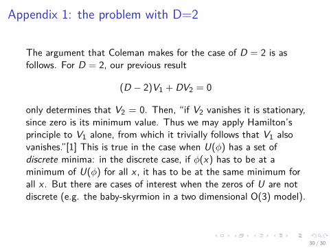
Appendix 1: the problem with D=2

The argument that Coleman makes for the case of D = 2 is asfollows. For D = 2, our previous result

(D − 2)V1 + DV2 = 0

only determines that V2 = 0. Then, “if V2 vanishes it is stationary,since zero is its minimum value. Thus we may apply Hamilton’sprinciple to V1 alone, from which it trivially follows that V1 alsovanishes.”[1] This is true in the case when U(φ) has a set ofdiscrete minima: in the discrete case, if φ(x) has to be at aminimum of U(φ) for all x , it has to be at the same minimum forall x . But there are cases of interest when the zeros of U are notdiscrete (e.g. the baby-skyrmion in a two dimensional O(3) model).

30 / 30