Introduction - igt.uni-stuttgart.de
34
DEFORMATIONS OF NEARLY PARALLEL G 2 -STRUCTURES B. ALEXANDROV, U. SEMMELMANN Abstract. We study the infinitesimal deformations of a proper nearly parallel G 2 -structure and prove that they are characterized by a certain first order differential equation. In par- ticular we show that the space of infinitesimal deformations modulo the group of diffeomor- phisms is isomorphic to a subspace of co-closed Λ 3 27 -eigenforms of the Laplace operator for the eigenvalue 8scal /21. We give a similar description for the space of infinitesimal Ein- stein deformations of a fixed nearly parallel G 2 -structure. Moreover we show that there are no deformations on the squashed S 7 and on SO(5)/SO(3), but that there are infinitesimal deformations on the Aloff-Wallach manifold N (1, 1) = SU(3)/U (1). 1. Introduction A nearly parallel G 2 -structure on a 7-dimensional manifold M is given by a 3-form σ of special algebraic type satisfying the differential equation *dσ = τ 0 σ for some constant τ 0 . Such a manifold has a structure group contained in the exceptional Lie group G 2 ⊂ SO(7) and, in particular, a Riemannian metric g induced by σ. It can be shown that nearly parallel G 2 -manifolds are irreducible and Einstein with scalar curvature scal = 21 8 τ 2 0 . Moreover, the existence of such a structure is equivalent to the existence of a spin structure with a Killing spinor. Another equivalent description of nearly parallel G 2 -structures is in terms of the metric cone ( ˆ M, ˆ g), which has to have holonomy contained in Spin(7), considered as subgroup of SO(8). The metric cone is the manifold ˆ M = M × R + with the warped product metric ˆ g = r 2 g ⊕ dr 2 . If (M 7 ,g) is simply connected and not isometric to the standard sphere, then there are three possible cases: the holonomy of ( ˆ M, ˆ g) is contained in Sp(2), equivalently, (M 7 ,g) is a 3-Sasakian manifold, the holonomy can be SU(4), equivalently, (M 7 ,g) is an Einstein-Sasaki manifold, or the holonomy is precisely Spin(7), in which case we call the G 2 -structure proper. We recall that these three cases correspond to the existence of a 3-, 2- resp. 1-dimensional space of Killing spinors. Proper nearly parallel G 2 -structures are also characterized by the vanishing of the Lie derivative L ξ σ for any Killing vector field ξ . In this article we shall mainly consider the case of proper nearly parallel G 2 -manifolds. In [12] it is shown that any 7-dimensional 3-Sasakian manifold admits a second nearly parallel G 2 -structure which is proper. The corresponding Einstein metric belongs to the metrics of the canonical variation of the 3-Sasakian Einstein metric. Applying this construction to The first author was partially supported by Contract 195/2010 with Sofia University ”St. Kl. Ohridski”. 1
Transcript of Introduction - igt.uni-stuttgart.de
DEFORMATIONS OF NEARLY PARALLEL G2-STRUCTURES
B. ALEXANDROV, U. SEMMELMANN
Abstract. We study the infinitesimal deformations of a proper nearly parallel G2-structureand prove that they are characterized by a certain first order differential equation. In par-ticular we show that the space of infinitesimal deformations modulo the group of diffeomor-phisms is isomorphic to a subspace of co-closed Λ3
27-eigenforms of the Laplace operator forthe eigenvalue 8scal /21. We give a similar description for the space of infinitesimal Ein-stein deformations of a fixed nearly parallel G2-structure. Moreover we show that there areno deformations on the squashed S7 and on SO(5)/SO(3), but that there are infinitesimaldeformations on the Aloff-Wallach manifold N(1, 1) = SU(3)/U(1).
1. Introduction
A nearly parallel G2-structure on a 7-dimensional manifold M is given by a 3-form σ ofspecial algebraic type satisfying the differential equation ∗dσ = τ0σ for some constant τ0.Such a manifold has a structure group contained in the exceptional Lie group G2 ⊂ SO(7)and, in particular, a Riemannian metric g induced by σ. It can be shown that nearly parallelG2-manifolds are irreducible and Einstein with scalar curvature scal = 21
8τ 2
0 . Moreover, theexistence of such a structure is equivalent to the existence of a spin structure with a Killingspinor.
Another equivalent description of nearly parallel G2-structures is in terms of the metriccone (M, g), which has to have holonomy contained in Spin(7), considered as subgroup of
SO(8). The metric cone is the manifold M = M × R+ with the warped product metricg = r2g ⊕ dr2. If (M7, g) is simply connected and not isometric to the standard sphere, then
there are three possible cases: the holonomy of (M, g) is contained in Sp(2), equivalently,(M7, g) is a 3-Sasakian manifold, the holonomy can be SU(4), equivalently, (M7, g) is anEinstein-Sasaki manifold, or the holonomy is precisely Spin(7), in which case we call theG2-structure proper. We recall that these three cases correspond to the existence of a 3-, 2-resp. 1-dimensional space of Killing spinors. Proper nearly parallel G2-structures are alsocharacterized by the vanishing of the Lie derivative Lξσ for any Killing vector field ξ.
In this article we shall mainly consider the case of proper nearly parallel G2-manifolds. In[12] it is shown that any 7-dimensional 3-Sasakian manifold admits a second nearly parallelG2-structure which is proper. The corresponding Einstein metric belongs to the metricsof the canonical variation of the 3-Sasakian Einstein metric. Applying this construction to
The first author was partially supported by Contract 195/2010 with Sofia University ”St. Kl. Ohridski”.
1
2 B. ALEXANDROV, U. SEMMELMANN
the homogeneous 3-Sasakian spaces S7 and N(1, 1) one obtains homogeneous proper nearlyparallel G2-structures: the squashed 7-sphere and the second Einstein metric on N(1, 1).The Aloff-Wallach spaces N(k, l) for (k, l) 6= (1, 1) also have exactly two nearly parallel G2-structures, both of which are proper. A further example is the isotropy irreducible spaceSO(5)/SO(3). In fact, due to the classification [12] these are the only homogeneous nearlyparallel G2-manifolds.
As a last remarkable property of nearly parallel G2-manifolds we mention the existence of ametric connection ∇ with totally skew-symmetric torsion. The so-called canonical connection∇ is defined as ∇ = ∇− τ0
12σ and has holonomy contained in the group G2 ⊂ SO(7). Nearly
parallel G2-manifolds appear as one of two exceptional cases in a classification of metricconnections with parallel torsion due to Cleyton and Swann [7]. The other exceptional caseis the class of 6-dimensional nearly Kahler manifolds, which turns out to be in various waysrather similar to nearly parallel G2-manifolds. The defining condition is the existence of anearly parallel almost complex structure J , i.e., J satisfying (∇XJ)(X) = 0 for any vectorfield X. Nearly Kahler manifolds in dimension 6 are also Einstein manifolds admitting aKilling spinor. Moreover, the metric cone has holonomy contained in G2.
In this article we shall show that nearly parallel G2-manifolds are also in another respectvery similar to nearly Kahler manifolds: the description of infinitesimal deformations. In [16]the space of infinitesimal nearly Kahler deformations is identified with the space of primitiveco-closed (1, 1)-eigenforms of the Laplace operator for the eigenvalue 2scal /5, [19] containsa similar description of the space of infinitesimal Einstein deformations. This space turnsout to be the sum of three such eigenspaces. Finally, in [18] it is shown that infinitesimaldeformations for the known homogenous examples only exist in the case of the flag manifoldSU(3)/T2. For all three results we shall obtain a counterpart on nearly parallel G2-manifolds.
We start with the equations of R. Bryant (cf. Proposition 3.1 and [6]) describing theinfinitesimal deformation of an arbitrary G2-structure. They give equations for the tangentvector on a curve of G2-structures. Specializing to the case of nearly parallel G2-structuresand staying transversal to the action of the diffeomorphism group, we obtain that the space ofsuch deformations is a direct sum of two spaces, D1 and D3, consisting of 1-forms and 3-formsrespectively. As shown in Section 4, the space D1 parametrizes Einstein-Sasakian structurescompatible with the given nearly parallel G2-structure. The more interesting space is D3
which consists of the solutions φ in Λ327T∗M of the differential equation ∗dφ = −τ0φ. In
particular, infinitesimal deformations φ ∈ D3 are co-closed and eigenforms of the Hodge-Laplace operator for the eigenvalue τ 2
0 = 8scal /21. But more important for the computation
in examples is that they are also eigenforms for the eigenvalue5τ206
of the G2-Laplace operator∆ introduced in Section 5. In Section 6 we describe the space of infinitesimal Einsteindeformations of the metric of a nearly parallel G2-structure. In addition to D3 one obtainstwo other spaces of sections of Λ3
27T∗M which are characterized by similar equations. In thelast section we compute the infinitesimal Einstein deformations of the normal homogeneousexamples: the isotropy irreducible space SO(5)/SO(3), the squashed 7-sphere and the second
DEFORMATIONS OF NEARLY PARALLEL G2-STRUCTURES 3
Einstein metric on the Aloff-Wallach space N(1, 1). We show that there exist no Einsteindeformations and, in particular, no deformations of the nearly parallel G2-structure in thefirst two cases, while in the third the space of infinitesimal Einstein deformations coincideswith the space of infinitesimal nearly parallel G2-deformations and is 8-dimensional. We donot know whether these infinitesimal deformations integrate to real Einstein deformations.
2. Preliminaries
Let e1, . . . , e7 denote the standard basis of R7 and e1, . . . , e7 its dual basis. On R7 we fixthe canonical scalar product 〈·, ·〉 and the standard orientation. We shall write ei1...ik for thewedge product ei1 ∧ . . . ∧ eik ∈ Λk(R7)∗ and define the fundamental 3-form as
(2.1) σ = e123 + e145 + e246 + e347 − e167 + e257 − e356.
The exceptional group G2 is defined as the subgroup of GL(7,R) that fixes the 3-form σ,i.e., G2 = g ∈ GL(7,R) | g∗σ = σ. The group G2 is a 14-dimensional compact, connected,simple Lie group, which acts irreducibly on T := R7 and preserves the metric, the orientationand the Hodge dual of σ, i.e. the 4-form
(2.2) ∗σ = e4567 + e2367 + e1357 + e1256 − e2345 + e1346 − e1247.
The irreducible representations of G2 can be indexed by their highest weights, which arepairs of non-negative integers (p, q) if written as linear combinations of the two fundamentalweights. The corresponding representation will be denoted by Vp,q. In this paper we will inparticular be interested in the following four irreducible G2-representations: the trivial rep-resentation V0,0 = R, the standard representation V1,0 = T := R7, the adjoint representationV0,1 = g2 and the representation on traceless symmetric 2-forms V2,0 = S2
0T∗. Among theirreducible representations these are uniquely determined by their dimensions 1, 7, 14 and27 respectively. Therefore we shall use the dimensions as lower indices when we decomposethe space of k-forms ΛkT∗ into irreducible components. In other words, Λk
r will denote ther-dimensional irreducible subspace of ΛkT∗. With this notation we have
(2.3) Λ2 = Λ2T∗ = Λ27 ⊕ Λ2
14, Λ3 = Λ3T∗ = Λ31 ⊕ Λ3
7 ⊕ Λ327,
with an isomorphic decomposition for Λ4T∗ ∼= Λ3T∗ and Λ5T∗ ∼= Λ2T∗ obtained with thehelp of the Hodge ∗-operator. The one-dimensional spaces in Λ3 resp. Λ4 are spanned by σresp. ∗σ. The space Λ2
14 is isomorphic to the Lie algebra of G2 and the other subspaces canbe characterized by
Λ27 = Xyσ ∈ Λ2 | X ∈ T ∼= T, Λ3
7 = Xy ∗ σ ∈ Λ3 | X ∈ T ∼= T,
Λ327 = α ∈ Λ3 | α ∧ σ = 0 = α ∧ ∗σ ∼= V2,0.
In the sequel we shall use the following G2-equivariant isomorphisms, which were introducedby Bryant in [6]: i : S2
0T∗ → Λ327 and j : Λ3
27 → S20T∗, where i is the restriction to S2
0T∗ ⊂ S2T∗
of the map S2T∗ → Λ3T∗, defined on decomposable elements by
α β 7→ α ∧ (βyσ) + β ∧ (αyσ),
4 B. ALEXANDROV, U. SEMMELMANN
while j is given by
j(γ)(X, Y ) = ∗((Xyσ) ∧ (Y yσ) ∧ γ).
Note that j = −8i−1. With the help of i one can obtain explicit elements of Λ327, e.g.
(2.4) i(e1 e2) = e146 + e157 + e245 − e267.
Because of T∗ ⊗ T∗ = S2T∗ ⊕ Λ2T∗ we have the following decomposition:
(2.5) V1,0 ⊗ V1,0∼= R⊕ V2,0 ⊕ V1,0 ⊕ V0,1.
Later we shall also need the decompositions
(2.6) V1,0 ⊗ V2,0∼= V1,0 ⊕ V2,0 ⊕ V0,1 ⊕ V1,1 ⊕ V3,0,
(2.7) V1,0 ⊗ V0,1∼= V1,0 ⊕ V2,0 ⊕ V1,1.
The group G2 can also be defined as the stabilizer of the vector cross product P , given by
(2.8) σ(X, Y, Z) = 〈P (X, Y ), Z〉,
where X, Y, Z are any vectors in T. Recall from [8] that a 2-fold vector cross product P is abilinear map P : T× T→ T satisfying for all X, Y ∈ T the equations
(2.9) 〈P (X, Y ), X〉 = 〈P (X, Y ), Y 〉 = 0 and ‖P (X, Y )‖2 = ‖X‖2‖Y ‖2 − 〈X, Y 〉2.
In particular, it follows from the second equation of (2.9) that P is skew-symmetric. Thuswe can consider P as a linear map P : Λ2T → T and write P (X ∧ Y ) = P (X, Y ). In thisnotation the second equation of (2.9) reads: ‖P (X ∧ Y )‖2 = ‖X ∧ Y ‖2. We also refer to [8]for the following relations satisfied by a general 2-fold vector cross product:
Lemma 2.1. For X, Y, Z ∈ T we have
(1) 〈P (X, Y ), Z〉 = 〈X,P (Y, Z)〉,(2) P (X,P (X, Y )) = −‖X‖2Y + 〈X, Y 〉X,(3) 2P (P (X, Y ), Z) = P (P (Y, Z), X) + P (P (Z,X), Y ) + 3〈X,Z〉Y − 3〈Y, Z〉X.
From now on we will usually identify vectors and 1-forms via the metric and denote withei, i = 1, . . . , 7 an orthonormal basis of T. For later use we still note
Lemma 2.2. Let X and Y be any vectors in T. Then the following equations hold
(X yσ) ∧ σ = −2X ∧ ∗σ,(2.10)
(X yσ) ∧ ∗σ = 3 ∗X,(2.11) ∑i (ei yX yσ) y (ei ∧ σ) = 3X y ∗ σ,(2.12) ∑i (ei yX yσ) ∧ (eiyσ) = 3X y ∗ σ,(2.13)
(X yY yσ) yσ + X yY y ∗ σ = −X ∧ Y,(2.14)
P (X yσ) = 3X.(2.15)
DEFORMATIONS OF NEARLY PARALLEL G2-STRUCTURES 5
The GL7-orbit of σ in Λ3T∗ is an open set by dimensional reasons. As usual it is denotedwith Λ3
+. Forms in Λ3+ are called stable or definite.
Let M be a 7-dimensional manifold. The union of the subspaces Λ3+T∗xM , x ∈M , of stable
forms defines an open subbundle Λ3+T∗M ⊂ Λ3T∗M . There is a one-to-one correspondence
between G2-structures on M , i.e. reductions of the structure group of M to the group G2,and the space of sections of Λ3
+T∗M , which we will denote with Ω3+(M). The defining 3-form
σ ∈ Ω3+(M) determines a Riemannian metric g and an orientation of M via the relation
(2.16) −6g(X, Y ) ∗ 1 = Xyσ ∧ Y yσ ∧ σ
(∗1 denotes the volume form). Let ∇ be the Levi-Civita connection of g. Then the covariantderivative ∇σ is a section of the bundle T∗⊗g⊥2 , where g⊥2
∼= T∗ is the orthogonal complementof g2 in Λ2T∗ and we identify bundles with the G2-representation defining it. It follows from(2.5) that this bundle decomposes as R⊕V2,0⊕V1,0⊕V0,1 and thus the covariant derivative ofσ has four components. Accordingly, one has the 16 Fernandez-Gray classes of G2-structures,with the four basic classes W1,W2,W3,W4 corresponding to the four irreducible summands.
In this article we shall consider the class W1 of so called nearly parallel (or weak) G2-structures, i.e. G2-structures induced by a non-parallel 3-form σ ∈ Ω3
+(M), such that ∇σis a section of the 1-dimensional subbundle defined by the trivial G2-representation. Nearlyparallel G2-structures can be described by several equivalent conditions in terms of σ.
Proposition 2.3. Let M be a 7-dimensional manifold with a G2-structure defined by a 3-formσ ∈ Ω3
+(M). Then the following conditions are equivalent
(1) The 3-form σ defines a nearly parallel G2-structure.(2) The 3-form σ is a Killing 3-form, i.e. ∇σ = 1
4dσ.
(3) There exists a τ0 ∈ R \ 0 with ∇σ = τ04∗ σ.
(4) There exists a τ0 ∈ R \ 0 with ∇X(∗σ) = − τ04X ∧ σ for all vector fields X.
(5) There exists a τ0 ∈ R \ 0 with dσ = τ0 ∗ σ.(6) Xy∇Xσ = 0 holds for all vector fields X.
Proof: The equivalence of (3) and (4) is obvious, while the equivalence of (1), (2), (3) and(6) has been proved in [8]. The only point not mentioned there is that τ0 is constant. This factis also known (see e.g. [12]) and can be proven as follows. Since (5) is an obvious consequenceof (3), we can differentiate it to obtain dτ0 ∧ ∗σ = 0, which implies dτ0 = 0. Finally, that (5)implies the remaining conditions was proved in [12]. This is the only point where one usesthat τ0 is different from zero.
Let P be the associated vector cross product, defined in (2.8). Then the condition (6) ofthe proposition above is equivalent to (∇XP )(X, Y ) = 0 for any vector fields X, Y , i.e., to Pbeing nearly parallel [13]. Further straightforward consequences of Proposition 2.3 in the caseof nearly parallel G2-manifolds are: d∗σ = 0 and ∆σ = τ 2
0 σ, where here and in the following∆ = dd∗+ d∗d denotes the Hodge-de Rham Laplacian. Moreover it follows that σ is a specialKilling 3-form, i.e. the additional equation ∇Xdσ = −1
4τ 2
0X∗ ∧ σ is satisfied for all vector
fields X (cf. [20]).
6 B. ALEXANDROV, U. SEMMELMANN
The canonical connection ∇ of a G2-structure is the unique G2-connection whose torsionis equal to the intrinsic torsion of the G2-structure. In the nearly parallel case it has totallyskew-symmetric and parallel torsion and is explicitly given by
(2.17) g(∇XY, Z) = g(∇XY, Z) − τ012σ(X, Y, Z)
or, equivalently, by
(2.18) ∇X = ∇X − τ012PX ,
where the endomorphism PX is defined by PXY := P (X, Y ).
Remark 2.4. The fact that P is G2-invariant allows the following important application,which we shall use several times in this article. Let V be an irreducible G2-representationcontained in some tensor space and VM be the corresponding associated bundle. Thenthe endomorphism PX extends to an endomorphism of VM and we may consider the G2-equivariant map V → T∗ ⊗ V , defined by ϕ 7→
∑i ei ⊗ Peiϕ, which we again denote by P .
By (2.18) we have(∇ − ∇)ϕ = − τ0
12Pϕ
for any section ϕ of VM . Let U be an irreducible component in T∗ ⊗ V . Suppose firstthat U is not isomorphic to V as a G2-representation. Then there exists no non-zero G2-equivariant map from V to U and therefore the UM -part (Pϕ)UM of Pϕ vanishes, whichimplies (∇ϕ)UM = (∇ϕ)UM . On the other hand, if U is isomorphic to V , then U = i(V ),where i : V → T∗ ⊗ V is some G2-equivariant embedding. Let π : T∗ ⊗ V → U be theprojection. Then π P : V → U is also G2-equivariant and therefore by Schur’s lemmaπ P = ci for some constant c. Thus (∇ϕ)i(VM) = (∇ϕ)i(VM) + cτ0
12i(ϕ). Finally, since ∇ϕ
and Pϕ are sections of T∗M ⊗ VM , the same is true for ∇ϕ, despite the fact that ∇ is nota G2-connection.
Remark 2.5. Our choice of the orientation induced by a stable 3-form σ is the opposite ofthe choice of Bryant in [6]. As a consequence our ∗, j, τ0 and f1 from the next section differfrom those in [6] by a sign.
3. Deformations of G2-structures
In this section we will consider a smooth curve σt of nearly parallel G2-structures anddescribe its tangent vector σ in t = 0. Here and in the sequel the dot denotes the timederivative at t = 0. As a starting point we use the following result of R. Bryant [6] for curvesof arbitrary G2-structures (cf. also [14]).
Proposition 3.1. Let (M7, g) be a Riemannian manifold with a family σt ∈ Ω3+(M) of G2-
structures. Let gt be the family of metrics and ∗t the Hodge star operator associated withσt. Then there exist three time-dependent differential forms f0 ∈ Ω0(M), f1 ∈ Ω1(M) andf3 ∈ Ω3
27(M) that satisfy the equations
(1) σ = 3 f0 σ + ∗(f1 ∧ σ) + f3,
(2) g = 2 f0 g − 12j(f3),
DEFORMATIONS OF NEARLY PARALLEL G2-STRUCTURES 7
(3) ∗σ = 4 f0 ∗ σ + f1 ∧ σ − ∗f3,
(4) ∗1 = 7 f0 ∗ 1.
Our aim is to study deformations of a given nearly parallel G2-structure σ on a compactmanifold M by nearly parallel G2-structures σt. We will only be interested in deformationsof the nearly parallel G2-structures modulo the action of the group R∗ ×Diff(M), given by
(λ, ϕ) · σ = λ3ϕ(σ) = λ3(ϕ−1)∗σ ϕ.
If σ induces the metric g, the Hodge dual ∗σ and the volume form ∗1, then σ = λ3σ induces
(3.19) g = λ2g, ∗σ = λ4 ∗ σ, ∗1 = λ7 ∗ 1, τ0 =1
λτ0.
Therefore we can always assume that the volume of M with respect to g is normalized.Moreover, we can apply the Ebin’s Slice Theorem and assume that gt is a curve in the slicethrough g. A nearly parallel G2-structure is Einstein with scalar curvature
(3.20) scal g = 218τ 2
0 .
Thus g is an infinitesimal Einstein deformation of g and by the theorem of Berger-Ebin (see[3], Chapter 12) we have
(3.21) tr g = 0, δ g = 0, ∆Lg = 2scal7g = 3
4τ 2
0 g,
where ∆L is the Lichnerowicz Laplacian (see [3] or Section 6 below). Since tr g = 14 f0, itimmediately follows that f0 vanishes and the equations of Proposition 3.1 may be rewrittenas
(3.22) σ = ∗(f1 ∧ σ) + f3, g = −12j(f3), ∗σ = f1 ∧ σ − ∗f3, ∗1 = 0,
while equations (3.21) become
(3.23) δ j(f3) = 0, ∆L j(f3) = 34τ 2
0 j(f3).
The fact that σt is a family of nearly parallel G2-structures means by definition that
(3.24) dσt = τ0(t) ∗ σtfor some function τ0(t). However, gt is a family of Einstein metrics and therefore scal gt isconstant as function in t, as follows from Corollary 2.12 of [3]. This, together with (3.20),implies that the function τ0 is constant too. Thus, differentiating (3.24) with respect to t, weobtain the linearized equation dσ = τ0 ∗σ, which by (3.22) yields
(3.25) d ∗ (f1 ∧ σ) + df3 = τ0(f1 ∧ σ − ∗f3).
The discussion above motivates the following definition.
Definition 3.2. An infinitesimal (nearly parallel) deformation of a compact nearly parallelG2-manifold (M,σ) is a section (f1, f3) of the bundle Λ1T∗M ⊕ Λ3
27T∗M , which satisfies theequations from (3.23) and (3.25).
8 B. ALEXANDROV, U. SEMMELMANN
The rest of this section is devoted to deriving a more explicit description of the space of in-finitesimal deformations of nearly parallel G2-structures. In a first step we obtain informationabout the 3-form component f3 of the infinitesimal deformation.
Lemma 3.3. The covariant derivatives of f3 with respect to ∇ and ∇ have no componentin T ⊂ T∗ ⊗ Λ3
27, i.e., it holds (∇f3)T = (∇f3)T = 0. In particular, the differential andcodifferential of f3 satisfy the equations:
(df3)Λ41
= 0, (df3)Λ47
= 0, (d∗f3)Λ27
= 0, (d ∗ f3)Λ57
= 0.
Proof: The divergence δ is defined as the composition of the covariant derivative ∇ and theequivariant contraction c : T∗⊗S2
0T∗ → T∗. It follows from Remark 2.4 and the decomposition(2.6) that (∇j(f3))T = (∇j(f3))T and (∇f3)T = (∇f3)T. This implies
(3.26) δj(f3) = −c∇j(f3) = −c(∇j(f3))T = −c(∇j(f3))T = −c (1⊗ j)(∇f3)T,
where the last equality follows from j being G2-equivariant and ∇-parallel. Since c (1 ⊗ j)is non-zero on T ⊂ T∗⊗Λ3
27 (which can be checked on an explicit element), we finally obtainδj(f3) = 0 if and only if (∇j(f3))T = (∇f3)T = 0.
By the definition of the differential we have df3 = ε∇f3, with the G2-equivariant wedgingmap ε : T∗ ⊗ Λ3T∗ → Λ4T∗. Again by (2.6) and Remark 2.4 we see that ∇f3 has no compo-nents in bundles associated with the trivial representation R. Thus df3 has no components inΛ4
1, which proves the first equation for df3. The second follows from (df3)Λ47
= ε(∇f3)T = 0and the remaining two are proved in a similar way.
In the next step we will derive information about the 1-form part of infinitesimal deformations.
Proposition 3.4. For the 1-form f1 the following holds:
(1) ∇f1 = −13τ0 f1 yσ.
(2) ∇f1 = −14τ0 f1 yσ.
(3) f1 is a Killing 1-form and df1 = −12τ0 f1 yσ. In particular, d∗f1 = 0 and (df1)Λ2
14= 0.
(4) d(f1 ∧ ∗σ) = −32τ0 ∗ f1, in particular d∗(f1 yσ) = −3
2τ0f1.
(5) ∆f1 = 34τ 2
0 f1.(6) d∗(f1 ∧ σ) = −τ0f1 y ∗ σ. In particular d ∗ (f1 ∧ σ) = τ0f1 ∧ σ.(7) f1 has constant length.
Proof: Statements (2) and (3) are obviously equivalent and (1) and (2) are equivalentbecause (2.17) implies ∇f1 = ∇f1 − τ0
12f1yσ. The remaining properties are consequences of
each of the first three. To prove (6) we use d∗f1 = 0, d∗σ = 0, (3) of Proposition 2.3 and(2.13) to obtain
d∗(f1∧σ) =∑∇eif1∧(eiyσ)−∇f]1
σ = −1
4τ0
∑(eiyf1yσ)∧(eiyσ)− 1
4τ0f1y∗σ = −τ0f1y∗σ.
Property (7) follows from
d|f1|2(X) = 2〈∇Xf1, f1〉 = −1
2τ0〈Xyf1yσ, f1〉 = −1
2τ0f1yXyf1yσ = 0.
DEFORMATIONS OF NEARLY PARALLEL G2-STRUCTURES 9
For the proof of (3) we start with computing the Λ27 part of df1. Since τ0 is a non-zero
constant we may take the differential of equation (3.25) to obtain d(f1 ∧ σ) = d ∗ f3. Now,let β be the 1-form, defined by (df1)Λ2
7= βyσ. Then the vanishing of the Λ5
7-part of d ∗ f3
and equation (2.10) imply
0 = (d(f1 ∧ σ))Λ57
= (df1)Λ27∧ σ − τ0f1 ∧ ∗σ = (βyσ) ∧ σ − τ0f1 ∧ ∗σ = (−2β − τ0f1) ∧ ∗σ.
Since the wedge product with ∗σ defines an injective map on 1-forms, we find β = −12τ0f1.
Hence (df1)Λ27
= −12τ0f1yσ. The Λ2
7-part of ∇f1 with respect to the decomposition (2.5) is12(df1)Λ2
7and we obtain (∇f1)Λ2
7= −1
4τ0f1yσ.
We continue with proving (4). Since the fundamental 3-form σ is coclosed, it followsd ∗ σ = 0. Moreover, the wedge product with ∗σ defines an equivariant map Λ2 → Λ6 ∼= Λ1,which by Schur’s Lemma vanishes on Λ2
14. Hence, using (2.11) we obtain
d(f1 ∧ ∗σ) = df1 ∧ ∗σ = (df1)Λ27∧ ∗σ = −1
2τ0(f1yσ) ∧ ∗σ = −3
2τ0 ∗ f1.
As an immediate consequence we obtain in addition d∗(f1 yσ) = −32τ0f1. Since τ0 6= 0, this
implies d∗f1 = 0.
Next we want to show that the Λ37-part of d(f1yσ) vanishes. Using Proposition 2.3 we
computed(f1yσ) =
∑i ei ∧∇ei(f1yσ) =
∑i ei ∧ (∇eif1yσ + f1y∇eiσ)
= −∑
i∇eif1y(ei ∧ σ) + (d∗f1)σ − f1ydσ +∇f]1σ
= −Φ(∇f1)− 34τ0f1y ∗ σ,
where Φ : Λ1 ⊗ Λ1 → Λ3 denotes the map Φ(γ) =∑
i(eiyγ)y(ei ∧ σ). Since Φ is obviouslyG2-invariant, we obtain
(d(f1yσ))Λ37
= −(Φ(∇f1))Λ37− 3
4τ0f1y∗σ = −Φ((∇f1)Λ2
7)− 3
4τ0f1y∗σ =
1
4τ0Φ(f1yσ)− 3
4τ0f1y∗σ.
Because (2.12) implies Φ(f1yσ) = 3f1y ∗ σ, we finally obtain
(3.27) (d(f1yσ))Λ37
= 0.
Now we shall prove the vanishing of the Λ214-part of df1 using the compactness of M . From
our equation for (df1)Λ27
we conclude
0 = d2f1 = d((df1)Λ27
+ (df1)Λ214
) = −12τ0d(f1yσ) + d(df1)Λ2
14.
From here it follows with (3.27) that (d(df1)Λ214
)Λ37
= 0. By definition the differential d is the
composition of the invariant wedging map ε : T ∗ ⊗ Λ2 → Λ3 and the covariant derivative ∇.By Remark 2.4 ∇γ is a section of T∗M ⊗ Λ2
14M for any section γ of Λ214M . Since by (2.7)
there is only one component isomorphic to T in T∗ ⊗ Λ214, we obtain for γ := (df1)Λ2
14:
0 = (dγ)Λ37
= πΛ37 ε∇γ = πΛ3
7 ε (∇γ)T.
Because πΛ37 ε is different from zero on T ⊂ T∗ ⊗ Λ2
14, as one checks on an explicit element,
this yields (∇γ)T = 0.
10 B. ALEXANDROV, U. SEMMELMANN
We may use a similar argument for the codifferential d∗, which is the composition of theinvariant contraction map c : T∗ ⊗ Λ2 → Λ1 and the covariant derivative. Hence we have
d∗γ = −c∇γ = −c (∇γ)T = 0.
Then the L2-scalar product of d∗γ and f1 yields
0 = (d∗γ, f1) = (γ, df1) = ‖γ‖2.
Thus it follows that γ = 0, i.e. (df1)Λ214
= 0, and that df1 is indeed a section of Λ27T∗M with
df1 = (df1)Λ27
= −12τ0f1 yσ.
We already know that f1 is coclosed and thus
∆f1 = d∗df1 = −12τ0d∗(f1yσ) = 3
4τ 2
0 f1,
which proves (5). Using the fact that the manifold (M7, g) is Einstein with scal = 218τ 2
0 ,we obtain ∆f1 = 2Ric(f1). By the well-known characterization of Killing vector fields oncompact manifolds this implies that f1 is Killing.
Finally we combine Proposition 3.4 with the initial equations to obtain a characterizationof infinitesimal deformations of nearly parallel G2-structures.
Theorem 3.5. The space of infinitesimal deformations of a compact nearly parallel G2-manifold (M,σ) is the direct sum of the finite-dimensional spaces
D1 := f1 ∈ Ω1(M) | ∇f1 = −14τ0 f1 yσ and D3 := f3 ∈ Ω3
27(M) | ∗ df3 = −τ0f3.In particular, f1 and f3 are co-closed eigenforms of the Laplace operator for the eigenvalues34τ 2
0 and τ 20 respectively.
Proof: It remains to prove the equations for f3. For this we substitute the expression ford ∗ (f1 ∧ σ) of Proposition 3.4 back into equation (3.25) and obtain df3 = −τ0 ∗ f3. Sinceτ0 6= 0 this immediately implies that f3 is coclosed. Then the Laplace operator is computedas ∆f3 = d∗df3 = (∗d)2f3 = τ 2
0 f3. It follows that an infinitesimal deformation lies in thedirect sum of the spaces D1 and D3. They are finite-dimensional since they are contained incertain eigenspaces of the Laplace operator.
Conversely, by Proposition 3.4 ∇f1 = −14τ0 f1 yσ and ∗df3 = −τ0f3 imply (3.25). Further,
df3 = −τ0 ∗ f3 yields (df3)Λ47
= 0, i.e., πΛ47 ε(∇f3)T = 0, where T ⊂ T∗ ⊗ Λ3
27 is the
component isomorphic to V1,0. Since πΛ47 ε is non-zero on T (which can be checked on an
explicit element), it follows that (∇f3)T = 0. Thus, by Remark 2.4 also (∇f3)T = 0 andtherefore by (3.26) δj(f3) = −c(1 ⊗ j)(∇f3)T = 0. It remains to show that ∗df3 = −τ0f3
implies ∆Lj(f3) = 34τ 2
0 j(f3), which will be done in Section 6.
4. G2-deformations and Sasakian structures
In this section we will investigate the relation between nearly parallel G2-manifolds with anon-trivial space D1 in Theorem 3.5 and Sasakian structures. The first result in this directionis the following.
DEFORMATIONS OF NEARLY PARALLEL G2-STRUCTURES 11
Proposition 4.1. Let (M, g, σ) be a compact nearly parallel G2-manifold normalized so thatτ0 = 4. Then:
(1) If dimD1 ≥ 1, then (M, g) is a Sasakian-Einstein manifold.(2) If dimD1 ≥ 2, then (M, g) is a 3-Sasakian manifold.
Proof: The assumption about the normalization is not a restriction because of (3.19). Let0 6= f1 ∈ D1, then Proposition 3.4 shows that f1 is a Killing 1-form of constant length andwe can assume |f1| = 1. Thus, to prove that f1 is the contact form of a Sasakian structure itremains (see [4]) to verify the curvature condition
(∇2X,Y f1)(Z) = f1(Y )g(X,Z) − f1(Z)g(X, Y ) = (f1 ∧X)(Y, Z)
However, taking the covariant derivative of the defining equation of D1 immediately implies:
(∇2X,Y f1)(Z) = −1
4τ0 (∇X(f1 yσ))(Y, Z) = −(∇Xf1 yσ)(Y, Z) − (f1 y∇Xσ)(Y, Z)
= 14τ0 ((Xyf1 yσ) yσ)(Y, Z) − 1
4τ0 (f1 yX y ∗ σ)(Y, Z) = (f1 ∧X)(Y, Z)
where we also used (2.14). Since g is known to be Einstein, we obtain the first statement.
If dimD1 ≥ 2, then (M, g) has two Sasakian structures, whose contact forms are linearlyindependent. This implies the second statement (see [4], Lemma 8.1.17).
Recall that a G2-structure on a 7-dimensional manifold M defines a canonical spin structureon M . The G2-structure is furthermore nearly parallel if and only if the associated spin struc-ture admits real Killing spinors [12]. In this case the nearly parallel G2-structures inducingthe given metric and spin structure are in bijective correspondence with the projectivizationof the space of Killing spinors in the real spinor bundle [12]. The complex spinor bundle isthe complexification of the real spinor bundle and the space of real Killing spinors is the com-plexification of the space of Killing spinors in the real spinor bundle, so both spaces have thesame dimension over the respective field. After a suitable normalization of the metric (whichin our case amounts to ensuring that τ0 = 4) this dimension is also equal to the dimension
of the space of parallel spinors on the metric cone M of M for the spin structure inducedby the one on M . This is a result of Bar [2] in the simply connected case and holds also ingeneral, as explained by Wang in [21]. Hence, as noticed in [2], if M is compact, then either
the restricted holonomy group of M is one of Spin(7), SU(4), Sp(2), or M is flat. In the lattercase M is a quotient of the standard sphere S7. According to a result of Friedrich [9], allnearly parallel G2-structures on S7 which induce the standard metric are conjugated underthe action of the isometry group. Thus neither S7 nor its quotients admit G2-deformations.Therefore from now on we shall exclude from our considerations the case of nearly parallelG2-manifolds with constant curvature. Under this assumption the compact nearly parallelG2-manifolds split into the following three different types.
Type 1. The space of real Killing spinors is 1-dimensional. Then there is only one 3-form inducing the given metric, orientation and spin structure. We call such nearly parallelG2-structures proper. Notice that our definition of a proper nearly parallel G2-structure isslightly different from those in [12] and [4]. In [12] one assumes additionally that the manifold
12 B. ALEXANDROV, U. SEMMELMANN
is simply connected, while the definition in [4] requires that the cone has holonomy equal toSpin(7). For simply connected manifolds the three definitions are equivalent.
Type 2. The space of real Killing spinors is 2-dimensional. Then the given metric andorientation are induced by a Sasaki-Einstein structure but not by a 3-Sasakian structure. Interms of the cone M this is equivalent to saying that the holonomy group of M is containedin SU(4) but not in Sp(2). Indeed, the subgroup of Spin(8) which acts as identity on a 2-dimensional subspace of one of the half-spin representations is Spin(6) ∼= SU(4). In this casethe 3-forms inducing the given metric, orientation and spin structure are parametrized byRP 1.
Type 3. The space of real Killing spinors is 3-dimensional. The given metric and orientationare induced by a 3-Sasakian structure. In terms of the cone M this is equivalent to sayingthat the holonomy group of M is equal to Sp(2). In this case the 3-forms inducing the givenmetric and orientation are parametrized by RP 2.
Now we shall describe the nearly parallel G2-structures of types 2 and 3 without referenceto Killing spinors. Recall that the cone of a Riemannian manifold (M, g) is (M, g), where
M := R+ ×M , g := dr2 + r2g and r is the natural coordinate on R+. As shown in [2], if wenormalize the nearly parallel G2-structure so that τ0 = 4, then σ = ∂ryϕ|r=1, where ϕ is aparallel (and also stable) 4-form on the cone.
Suppose first that the holonomy group of the cone is equal to SU(4) (which implies that M
is Sasaki-Einstein but not 3-Sasakian). Then the space of parallel 4-forms on M is spannedby ΩI ∧ ΩI , Re ΨI , Im ΨI . Here ΩI is the Kahler form and ΨI the complex volume form ofthe SU(4)-structure. Thus
σ = ∂ry
(1
2c0ΩI ∧ ΩI + c1Re ΨI + c2Im ΨI
)∣∣∣∣r=1
.
Equivalently, one can write this as
σ = c0η ∧ Ω + c1Re Ψ + c2Im Ψ,
where η is the contact form of the Sasaki-Einstein structure on M , Ω = ∇η is the hori-zontal Kahler form and Ψ is the horizontal complex volume form. Now a straightforwardcomputation using (2.16) shows that σ induces the given metric and orientation if and onlyif c0 = −1 and c2
1 + c22 = 1. Hence we have the following explicit S1-family of nearly parallel
G2-structures:
(4.28) σt = −η ∧ Ω + cos tRe Ψ + sin t Im Ψ.
In particular, each σt is of type 2.
Now suppose that the holonomy group of the cone is Sp(2) (i.e., M is a 3-Sasakian mani-fold). Then the space of parallel 4-forms is spanned by
ΩI1∧ ΩI1
, ΩI2∧ ΩI2
, ΩI3∧ ΩI3
, ΩI1∧ ΩI2
, ΩI2∧ ΩI3
, ΩI3∧ ΩI1
.
DEFORMATIONS OF NEARLY PARALLEL G2-STRUCTURES 13
Here ΩI1, ΩI2
, ΩI3are the Kahler forms of the hyper-Kahler structure I1, I2, I3 on the cone
(we use the convention I1I2 = −I3). Thus
σ = ∂ry
(1
2
∑λ
sλλΩIλ∧ ΩIλ
+∑λ<µ
sλµΩIλ∧ ΩIµ
)∣∣∣∣∣r=1
.
Equivalently, this can be written as
(4.29) σ =3∑
λ,µ=1
sλµηλ ∧ Ωµ
with sλµ = sµλ, where η1, η2, η3 are the contact forms of the 3-Sasakian structure on Mand Ωλ = ∇ηλ are the corresponding Kahler forms. Again a straightforward computationusing (2.16) shows that σ given by (4.29) induces the given metric and orientation if andonly if the matrix S = (sλµ) is in SO(3) and trS = −1. The condition sλµ = sµλ meansfurthermore that σ is nearly parallel if and only if S is symmetric. An orthogonal matrix issymmetric if and only if its eigenvalues are real and the condition trS = −1 implies that theyare 1,−1,−1. But an orthogonal matrix with eigenvalues 1,−1,−1 is completely determinedby its 1-eigenspace. Thus we obtain that the nearly parallel G2-structures are parametrizedby RP 2 (in particular, they are of type 3). We shall identify R3 with spanη1, η2, η3. Thenη ∈ spanη1, η2, η3 is the contact form of a Saskai-Einstein structure if and only if η lieson the unit sphere S2. Let S(η) = (sλµ(η)) denote the orthogonal matrix with eigenvalues1,−1,−1 whose 1-eigenspace is spanned by η. Then the nearly parallel G2-structures are
σS(η) =∑λ,µ
sλµ(η)ηλ ∧ Ωµ | η ∈ S2
(notice that S(η) = S(−η)).
Fixing an η, we can again write the S1-family ση,t from the SU(4)-case. Inside the RP 2-family it is identified by
ση,t = σS(η′) | η′ ∈ S2, η′ ⊥ η.This follows from the fact that ΨI1
= 12(ΩI2
− iΩI3) ∧ (ΩI2
− iΩI3), i.e.,
Re Ψ1 = η2 ∧ Ω2 − η3 ∧ Ω3, Im Ψ1 = −η2 ∧ Ω3 − η3 ∧ Ω2.
Finally, let the holonomy group Hol(M) of the cone lie strictly between SU(4) and Sp(2).
Then the restricted holonomy group is Sp(2) and therefore Hol(M) ⊂ Sp(2)Sp(1) as the
normalizer of Sp(2) in O(8) is Sp(2)Sp(1). Now the fact that Hol(M) preserves a complex
structure implies Hol(M) ⊂ Sp(2)U(1). Finally, Hol(M) preserves a complex volume form,
so the U(1) part of Hol(M) is contained in
a ∈ U(1) | a4 = 1 = 1, i,−1,−i = Z4.
Since Sp(2)Z2 = Sp(2), it remains Hol(M) = Sp(2)Z4. Now we have to find which Sp(2)-invariant 4-forms are also Sp(2)Z4-invariant. Notice that the action of i ∈ Z4 is in fact the
14 B. ALEXANDROV, U. SEMMELMANN
complex structure I = I1. Since I1 acts on ΩI1as the identity and on ΩI2
and ΩI3as minus
identity, the space of Sp(2)Z4-invariant 4-forms is 4-dimensional and is spanned by
ΩI1∧ ΩI1
, ΩI2∧ ΩI2
, ΩI3∧ ΩI3
, ΩI2∧ ΩI3
.
Now the results of the Sp(2)-case imply that σ is given by (4.29) with s12 = s21 = s13 = s31 =0. Thus either s11 = 1 and
σ = σS(η1) = η1 ∧ Ω1 − η2 ∧ Ω2 − η3 ∧ Ω3
or s11 = −1 and σ = σS(η′) for some η′ orthogonal to η = η1, i.e.,
σ = ση,t = −η ∧ Ω + cos tRe Ψ + sin t Im Ψ.
Thus in this case we have nearly parallel G2-structures of different types sharing the samemetric: σS(η1) is of type 1, while ση,t are of type 2.
Now we can prove the main result of this section.
Theorem 4.2. Let (M,σ) be a compact nearly parallel G2-manifold which is normalized sothat τ0 = 4 and is not a space of constant curvature. Then:
(1) (M,σ) is of type 1 if and only if dimD1 = 0.(2) (M,σ) is of type 2 if and only if dimD1 = 1.(3) (M,σ) is of type 3 if and only if dimD1 = 2.
Proof: Suppose that (M,σ) is of type 2. Then the holonomy of the cone is SU(4) orSp(2)Z4 ⊂ SU(4) and the consideration above show that σ is σt from (4.28) for some t. Againby Proposition 4.1 we have dimD1 ≤ 1. By definition, the contact form η of the Sasakianstructure satisfies ∇η = Ω. On the other hand, ηyσt = −Ω and therefore ∇η = −1
4τ0ηyσt.
Thus η ∈ D1, D1 = spanη and dimD1 = 1.
Let (M,σ) be of type 3. Then M is 3-Sasakian and the holonomy of the cone is Sp(2),so σ = σS(η) for some η ∈ S2. We shall show that D1 is the orthogonal complement of η inspanη1, η2, η3. Without loss of generality we can assume that η = η1 (otherwise we shallchange the orthonormal frame η1, η2, η3). Then σ ∈ ση2,t and σ ∈ ση3,t, so as aboveη2, η3 ∈ D1 and therefore dimD1 ≥ 2. By Proposition 4.1 every element of D1 induces aSasakian structure on (M, g) and by Lemma 8.1.17 in [4] it lies in spanη1, η2, η3. Thus, ifwe assume that dimD1 ≥ 3, we must have D1 = spanη1, η2, η3. But ∇η1 = Ω1, while S(η1)is the diagonal matrix with diagonal elements 1,−1,−1 and
−1
4τ0η1yσS(η1) = −η1y(η1 ∧ Ω1 − η2 ∧ Ω2 − η3 ∧ Ω3) = −Ω1 − η2 ∧ η1yΩ2 − η3 ∧ η1yΩ3
= −Ω1 − 2η2 ∧ η3 6= Ω1.
Hence η1 6∈ D1 and we have D1 = spanη2, η3 = η⊥1 and dimD1 = 2. This proves (3) sincethe reverse implication follows from Proposition 4.1.
Suppose now that dimD1 = 1. Then, by Proposition 4.1, (M, g) is Sasaki-Einstein but not3-Sasakian. Thus, to prove the reverse implication of (2) we only have to show that the case
Hol(M) = Sp(2)Z4 with σ = σS(η1) is impossible. Indeed, the proof of Proposition 4.1 yields
DEFORMATIONS OF NEARLY PARALLEL G2-STRUCTURES 15
that the contact form η1 must be an infinitesimal deformation of σS(η1) but in the type 3 caseabove we saw that this is not true. This completes the proof of (2).
Finally, (1) follows from Proposition 4.1, (2) and (3).
Remark 4.3. A nearly parallel G2-structure of type 2 is a part of a whole curve σt of suchstructures. It is easy to see that dσt
dt= ∗(η ∧ σt) (η is the contact form of the Sasaki-Einstein
structure). Let ξ be the vector field dual to η. Since all σt have τ0 = 4 and D1 = spanη,we obtain from Proposition 3.4 and Proposition 2.3 that
Lξσt = d(ξyσt) + ξydσt = −1
2d2η + 4ξy ∗ σt = −4 ∗ (η ∧ σt).
Let ϕs be the flow of ξ. Since ξ is Killing, ϕs preserves the metric and thus also η and ∗.Now the fact Lξσt = − dϕs(σt)
ds
∣∣∣s=0
and the above equations imply
dϕs(σt)
ds= 4 ∗ (η ∧ ϕs(σt)) =
dσt+4s
ds.
This and ϕ0(σt) = σt show that ϕs(σt) = σt+4s for all s. Thus the flow of ξ acts transitivelyon the family σt and so the members of this family are equivalent G2-structures.
In a similar way, if the type is 3, one can generate the whole D1 through curves in theRP 2-family σS(η). But this family consists of equivalent G2-structures since a 3-Sasakianmanifold admits an isometric SO(3) or Sp(1) action which is transitive on the oriented or-thonormal frames (η1, η2, η3) and therefore transitive also on the family σS(η).
Thus, whatever the type of the nearly parallel G2-structure, the ”interesting” infinitesimaldeformations are in the space D3.
Remark 4.4. We have seen above that if the holonomy group of the cone M is Sp(2)Z4, thenM has nearly parallel G2-structures of different type sharing the same metric and orientation.This is possible because they induce different spin structures on M and therefore also on M .Indeed, Sp(2)Z4 has two different embeddings in Spin(8). The first one, i1, is the restrictionon Sp(2)Z4 of the embedding of SU(4) in Spin(8). The second, i2, is equal to i1 on the identitycomponent of Sp(2)Z4 and to −i1 on the other component, i.e.,
i2([a, 1]) = i1([a, 1]), i2([a, i]) = −i1([a, i]) for a ∈ Sp(2).
Let E ∼= C4 be the standard representation of Sp(2). Then the spin representation, restrictedto Sp(2), is isomorphic to
∑4p=0 ΛpE. The action of i1(Sp(2)Z4) is given by
i1([a, z])α = zpaα for α ∈ ΛpE
and the space of invariant spinors is 2-dimensional: Λ0E ⊕ Λ4E. On the other hand, theaction of i2(Sp(2)Z4) is
i2([a, 1])α = aα, i2([a, i])α = −ipaα for α ∈ ΛpE
and the space of invariant spinors is 1-dimensional: CσE ⊂ Λ2E = CσE ⊕ Λ20E, where σE is
the Sp(2)-invariant symplectic form. Thus an 8-dimensional manifold with holonomy groupSp(2)Z4 is equipped with two canonical spin structures, one of which carries N = 2 and the
16 B. ALEXANDROV, U. SEMMELMANN
other N = 1 parallel spinors. Similarly, a 7-dimensional manifold whose cone has holonomygroup Sp(2)Z4 has two spin structures, withN = 2 andN = 1 real Killing spinors respectively.This adds to the results in [21], where in part 2b of Theorem 4.1 N = 1 is given as the onlypossibility, while the group Sp(2)Z4 is completely missing in part 3 of Corollary 5.2. Noticethat the existence of 7-dimensional manifolds with cones having holonomy group Sp(2)Z4 hasbeen proved in [17].
5. The G2-Laplace operator
In Section 3 we have seen that infinitesimal deformations of nearly parallel G2-manifoldsgive rise to coclosed eigenforms of the Hodge-de Rham Laplacian acting on sections ofΛ3
27T∗M . By the classical Weitzenbock formula the Hodge-de Rham Laplacian is writtenas
(5.30) ∆ = d∗d+ dd∗ = ∇∗∇+ q(R),
where q(R) is an endomorphism of the form bundle, which is linear in the curvature Rand satisfies q(R) = Ric on the space of 1-forms. We will define the operator q(R) inthe following more general setting. Let (M, g) be an n-dimensional Riemannian manifold.For a representation V of O(n) let VM denote the corresponding associated vector bundle.We denote the action of α ∈ Λ2T∗ ∼= so(n) on V by α∗ (here T denotes the standardrepresentation Rn of O(n)) and in a similar way the action of α ∈ Λ2T∗xM on VxM , x ∈ M .The endomorphism q(A) ∈ End (VM) is defined for any A ∈ Λ2T∗M ⊗ End (VM) by
(5.31) q(A) =∑i<j
(ei ∧ ej)∗A(ei ∧ ej),
where ei is a local orthonormal frame of TM . Notice that in this definition ei∧ej | i < j could be replaced by any other orthonormal basis of Λ2TM . The curvature R of the Levi-Civita connection ∇ or, more generally, the curvature R of any metric connection ∇ on (M, g)defines a section of Λ2T∗M ⊗ End (VM), thus the endomorphisms q(R) and q(R) are welldefined. We denote by ∆ the Laplace type operator
(5.32) ∆ := ∇∗∇+ q(R).
The operator ∆L := ∇∗∇ + q(R) for the Levi-Civita connection ∇ and a subrepresentationV ⊂ ⊗p T is also called Lichnerowicz Laplacian (cf. [3], Chapter 1 I). Because of (5.30) itcoincides on differential forms with the Hodge deRham Laplacian ∆.
Now let us return to the case of nearly parallel G2-manifolds. We will call the operator ∆,defined with the canonical connection ∇, the G2-Laplace operator. In order to compute thespectrum of the Lichnerowicz Laplacian ∆L on naturally reductive spaces, it turns out to beconvenient to express ∆L through ∆. Thus, our next aim will be to compute the difference∆−∆L, which we do by calculating the differences ∇∗∇ −∇∗∇ and q(R)− q(R) separately.
DEFORMATIONS OF NEARLY PARALLEL G2-STRUCTURES 17
A direct calculation using (2.18) and the third equation of Lemma 2.1 gives
RX,YZ −RX,YZ = ( τ012
)2 [2P (P (X, Y ), Z) + P (P (Y, Z), X) + P (P (Z,X), Y )]
= ( τ012
)2 [4P (P (X, Y ), Z)− 3g(X,Z)Y + 3g(Y, Z)X].
Thus R(X ∧ Y )−R(X ∧ Y ) = ( τ012
)2 [4PP (X∧Y )− 3(X ∧ Y )∗]. Substituting this equation intothe definition of the curvature endomorphisms q(R) and q(R), we obtain
(5.33) q(R) − q(R) = −3( τ012
)2 Cas so(7) + 4( τ012
)2 S
where Cas so(n) is the so(n)-Casimir operator∑
i<j(ei ∧ ej)∗(ei ∧ ej)∗ and S is defined as
(5.34) S =∑i<j
(ei ∧ ej)∗PP (ei∧ej).
Since P : Λ2T ∼= Λ27 ⊕ Λ2
14 → T is a G2-equivariant map, P |Λ214
= 0 and we may replace in
the sum in (5.34) the orthonormal basis ei ∧ ej | i < j of Λ2T with the orthonormal basisfi = 1√
3eiyσ | i = 1, . . . , 7 of Λ2
7. Because obviously fi∗ = 1√3(eiyσ)∗ = 1√
3Pei and, by
(2.15), P (fi) =√
3 ei, we obtain S =∑fi∗PP (fi) =
∑PeiPei . For the difference ∇∗∇ −∇∗∇
of the two rough Laplacians we derive directly from (2.18)
∇∗∇ − ∇∗∇ =∑(
τ06Pei∇ei + ( τ0
12)2PeiPei
).
Summarizing these calculation we obtain an expression for the difference of ∆ and ∆L.
Proposition 5.1. The difference of the Laplace type operators ∆ and ∆L on a nearly parallelG2-manifold is given by
(5.35) ∆ − ∆L = τ06
∑Pei∇ei − 3( τ0
12)2Cas so(7) + 5( τ0
12)2∑
PeiPei .
We shall apply this result for the space Λ327. Recalling that the so(n)-Casimir operator
acts as −p(n − p)id on the space of p-forms, we obtain Cas so(7)γ = −12γ for γ ∈ Λ327. A
straightforward computation on an explicit element (e.g. the element from (2.4)) shows thatthe G2-equivariant map
∑PeiPei acts as −8id on Λ3
27. Thus it remains to compute∑Pei∇ei .
The map∑Pei eiy : T∗ ⊗ Λ3
27 → Λ3 is G2-equivariant. Hence, because of (2.3) and (2.6),it can be non-zero only on the components of T∗ ⊗ Λ3
27 which are isomorphic to V1,0∼= T
and V2,0∼= Λ3
27. A straightforward computation on explicit elements shows that∑Pei eiy
is −3 ∗ ε on the component T ⊂ T∗⊗Λ327 and ∗ ε on the component Λ3
27 ⊂ T∗⊗Λ327. Here
again ε : T∗ ⊗ Λ3 → Λ4 denotes the wedging map. Thus∑Pei∇eiγ =
∑Pei eiy∇γ = −3 ∗ ε(∇γ)T + ∗ε(∇γ)Λ3
27= −3 ∗ (dγ)Λ4
7+ ∗(dγ)Λ4
27,
where d := ε ∇. Now, by (2.18) we have d = d− τ012
∑ei ∧Pei . Again a simple computation
on an element of Λ327 shows that
∑ei ∧ Pei = −2∗ on Λ3
27 and we eventually obtain
Lemma 5.2. On sections of Λ327T∗M it holds that d = d+ τ0
6∗. In particular, we have
(dγ)Λ47
= (dγ)Λ47, (dγ)Λ4
27= (dγ)Λ4
27+ τ0
6∗ γ, (dγ)Λ4
1= (dγ)Λ4
1= 0 for γ ∈ Ω3
27(M).
18 B. ALEXANDROV, U. SEMMELMANN
Using this lemma we obtain∑Pei∇eiγ = −3 ∗ (dγ)Λ4
7+ ∗(dγ)Λ4
27+ τ0
6γ, which finally enables
us to compute the difference ∆−∆ on Ω327(M). Combining the formulas above we find
Proposition 5.3. Let (M7, g, σ) be a nearly parallel G2-manifold and let γ be a 3-form inΩ3
27(M). Then
∆γ = ∆γ − τ02∗ (dγ)Λ4
7+ τ0
6∗ (dγ)Λ4
27.
In particular, ∆ and ∆ coincide on closed forms in Ω327(M). Moreover, if γ is a 3-form in
Ω327(M) with (d∗γ)Λ2
7= 0, then ∆γ = ∆γ + τ0
6∗ dγ.
Proof: It only remains to prove the last statement: Recall from the proof of Lemma 3.3,that for γ ∈ Ω3
27(M) the condition (d∗γ)Λ27
= 0 is equivalent to (dγ)Λ47
= 0 and thus, by
Lemma 5.2, also to (dγ)Λ427
= dγ. Substituting this into the equation for ∆ implies the laststatement.
6. Infinitesimal Einstein deformations
Nearly parallel G2-structures induce Einstein metrics and thus infinitesimal deformationsof such structures are related to infinitesimal Einstein deformations. In this section we shallconsider the space of infinitesimal Einstein deformations of a given nearly parallel G2-metricand realize it as a direct sum of certain spaces of 3-forms in Ω3
27(M).
Let g be an Einstein metric with Ric = Eg. From [3], Theorem 12.30, the space of infin-itesimal Einstein deformations of g is isomorphic to the set of trace-free symmetric bilinearforms h on TM with δh = 0 and ∆Lh = 2Eh, where ∆L = ∇∗∇ + q(R) is the so-calledLichnerowicz Laplacian (see the previous section). Note that for a nearly parallel G2-metric
the eigenvalue can be written as 2E = 2scal7
=3τ204
.
As a G2-representation the space S20T∗ is isomorphic to Λ3
27T. We shall now use the explicitidentification i in order to identify infinitesimal Einstein deformations with certain eigenformsof the Laplacian on forms in Λ3
27T. To do this we still need an analogue of Proposition 5.3.
We apply the results of Proposition 5.1 to the space S20T∗. It is well known that the so(n)-
Casimir operator acts on S20T∗ as −2nId, i.e., as −14Id in our case. Moreover it is clear that
similarly∑PeiPei , as a G2-equivariant map, acts as a multiple of the identity. An explicit
calculation, e.g. on the element e1 e2, shows that∑PeiPei = −14Id.
It remains to determine∑Pei∇eih, i.e., Q(∇h), where Q : T∗ ⊗ S2
0T∗ → S20T∗ is the
G2-equivariant map defined as Q =∑Pei eiy. The map Q is different from zero only on
the component of T ∗ ⊗ S20T∗, which is isomorphic to S2
0T∗. Let i2 : S20T∗ → T∗ ⊗ S2
0T∗ bethe embedding given as i2(h) = (1⊗ π0) C(g ⊗ h), where g is the metric, C : T∗⊗4 → T∗⊗3
is defined by C(a ⊗ b ⊗ c ⊗ d) = a ⊗ P (b, c) ⊗ d and π0 : T∗ ⊗ T∗ → S20T∗ denotes the
standard projection. Moreover, let π2 : T∗ ⊗ S20T∗ → S2
0T∗ be the projection ”inverse” to i2,i.e. π2 i2 = id and π2 vanishes on the components of T∗ ⊗ S2
0T∗ that are not isomorphicto S2
0T∗. Then an explicit calculation, e.g. on e1 e2, shows that Q i2 = −7id and thus
DEFORMATIONS OF NEARLY PARALLEL G2-STRUCTURES 19
Q = −7π2. Substituting this and the results for Cas so(7) and∑PeiPei into equation (5.35),
we obtain
(6.36) (∆−∆L)h = −7τ06π2(∇h) − 7τ20
36h.
Since S20T∗ and Λ3
27 are isomorphic representations of G2 and ∇ is a G2-connection, the bun-dles S2
0T∗M and Λ327M share the same G2-Laplace operator ∆, i.e., with the G2-equivariant
isomorphism i : S20T∗ → Λ3
27 we have i ∆ i−1 = ∆. Hence, to compute i ∆L i−1 weneed to compute i π2 ∇ i−1. An easy calculation shows that i = π1 (1 ⊗ i) i2, whereπ1 : T∗⊗Λ3
27 → Λ327 is defined as π1(α⊗ γ) = 2
7∗ (α∧ γ)Λ4
27. The map i2 π2 is the projection
on the component isomorphic to S20T∗ in T∗ ⊗ S2
0T∗ and since π1 (1 ⊗ i) is invariant withvalues in S2
0T∗, it vanishes on all other components of T∗ ⊗ S20T∗. Hence π1 (1⊗ i) = i π2
and we obtain from Lemma 5.2
(6.37) i π2(∇h) = π1 (1⊗ i)∇h = π1∇(i(h)) = 27∗ (di(h))Λ4
27= 2
7∗ (di(h))Λ4
27+ τ0
21i(h).
Let h be an infinitesimal Einstein deformation and let γ ∈ Ω327(M) denote the 3-form i(h).
Then the condition δh = 0 translates into (d∗γ)Λ27
= 0 or, equivalently, to dγ = (dγ)Λ427
.
Indeed, by Remark 2.4 we have that (∇h)T = (∇h)T and (∇γ)T = (∇γ)T. Thus δh = 0is equivalent to (∇h)T = 0 and also to (∇h)T = 0. But since i is an G2-equivariant map,(∇h)T = 0 if and only if (∇γ)T = 0, i.e., (∇γ)T = 0. However this is equivalent to (d∗γ)Λ2
7= 0
and also to (dγ)Λ47
= 0. Then by Lemma 5.2 (dγ)Λ47
= 0 can be written as dγ = (dγ)Λ427
.
Finally, we apply i to (6.36), use Proposition 5.3 and substitute (6.37) to obtain
Proposition 6.1. For each γ ∈ Ω327(M) the following equation is satisfied:
(6.38) i ∆L i−1(γ) = ∆γ − τ02∗ (dγ)Λ4
7+ τ0
2∗ (dγ)Λ4
27+
τ204γ.
With this formula we are able to translate the conditions for infinitesimal Einstein defor-mations into equivalent conditions for 3-forms in Ω3
27(M): The traceless symmetric bilinearform h is an infinitesimal Einstein deformation if and only if γ = i(h) is a section of Λ3
27T∗Mwith (dγ)Λ4
7= 0 (or, equivalently, (d∗γ)Λ2
7= 0), satisfying the equation
(6.39) ∆γ + τ02∗ dγ − τ20
2γ = 0.
We want to decompose the solution space of this equation into eigenspaces of the operator∗d. This is possible since ∗d is a symmetric operator, commuting with the operator on theleft hand side of equation (6.39) and preserving the condition (d∗γ)Λ2
7= 0. Indeed, ∗dα is
coclosed for any differential form α. Moreover, the solution space is finite dimensional becauseit is the kernel of an elliptic operator. Assume that ∗dγ = λγ with λ 6= 0. Then γ is coclosed(in particular, (d∗γ)Λ2
7= 0 and (dγ)Λ4
7= 0) and (6.39) yields the quadratic equation
(6.40) λ2 + τ02λ − τ20
2= 0
with the solutions λ = −τ0 and λ = τ02
. In the case λ = 0 we obtain dγ = 0 and dd∗γ =τ202γ.
Moreover a solution γ of the last equation is automatically closed and thus (dγ)Λ47
= 0 as well
as (d∗γ)Λ27
= 0. Summarizing we have
20 B. ALEXANDROV, U. SEMMELMANN
Theorem 6.2. Let (M, σ, g) be a compact nearly parallel G2-manifold. Then the space ofinfinitesimal Einstein deformations of g is isomorphic to the direct sum of the spaces
γ ∈ Ω327 | ∗ dγ = −τ0γ, γ ∈ Ω3
27 | ∗ dγ = τ02γ, γ ∈ Ω3
27 | dd∗γ =τ202γ.
Notice that the first space is the space D3 from Theorem 3.5. Thus any element f3 ∈ D3
satisfies i ∆Li−1 (f3) =3τ204f3, or, equivalently, ∆L j(f3) =
3τ204
j(f3), which finishes the proofof Theorem 3.5.
In order to check in the examples whether or not infinitesimal Einstein deformations existit will be convenient to embed these three spaces into eigenspaces of the operator ∆ acting onsections of Λ3
27T∗M . Let γ be a 3-form as above with ∗dγ = λγ for λ 6= 0. Then γ is coclosed
and ∆γ = λ2γ. Thus Proposition 5.3 implies ∆γ = (λ2 + τ06λ)γ. In the case dd∗γ =
τ202γ it
follows that γ is closed and we obtain ∆γ = ∆γ = dd∗γ =τ202γ. This proves
Lemma 6.3. The three summands of Theorem 6.2 are contained in the eigenspaces of ∆
acting on Ω327(M) for the eigenvalues
5τ206
,τ203
andτ202
respectively.
7. Naturally reductive spaces
In this section we will make some general remarks which will help us to compute the in-finitesimal Einstein deformations of nearly parallel G2-manifolds that are naturally reductivehomogenous spaces, i.e. reductive spaces where the torsion of the canonical homogenousconnection can be considered as a 3-form.
Lemma 7.1. Let G/H be a 7-dimensional oriented naturally reductive homogeneous spacewith reductive decomposition g = h⊕m. Suppose that at the initial point o the torsion of thecanonical homogeneous connection ∇ is To = − τ0
6σo with τ0 6= 0 and that σo is stable and
induces the given metric and orientation on m. Then σo defines by translations a G-invariant3-form σ and thus a G2-structure on G/H compatible with the given metric and orientation.
This G2-structure is nearly parallel and its canonical connection is ∇ = ∇. In particular,dσ = τ0 ∗ σ.
Moreover if G/H is standard up to a scaling factor c2, i.e., m is the orthogonal complementof h with respect to the Killing form B of g and the metric is induced by the restriction of−c2B to m, then the scalar curvature is scal = 63
20c2and τ 2
0 = 65c2
.
Proof: Since σo = − 6τ0
To is an H-invariant 3-form on m, σ = − 6τ0
T is a G-invariant 3-form
on G/H. In particular, σ is parallel with respect to the canonical homogeneous connection
∇ = ∇+ 12
T = ∇− τ012σ.
For X ∈ R7 we have the identity PXσ = 3Xy ∗ σ (which follows from (2.12) and (2.13) orby an explicit computation for some X 6= 0). Thus
∇Xσ = ∇Xσ + τ012PXσ = τ0
4X y ∗ σ
DEFORMATIONS OF NEARLY PARALLEL G2-STRUCTURES 21
and Proposition 2.3 implies that the G2-structure is nearly parallel with dσ = τ0∗σ. Moreover∇ coincides with the canonical connection ∇ of the G2-structure because of (2.18).
Suppose now that G/H is standard (up to a scaling factor c2). Obviously, it is enough to
prove the statement about the scalar curvature when c = 1. Recall that To(X, Y ) = −[X, Y ]mfor X, Y ∈ m. Then, considering again To as a 3-form and using (7.39) in [3], we obtain
scal = −64|To|2 + 7
2= − τ20
24|σo|2 + 7
2.
Since σo induces the metric on m we have |σo|2 = 7 and, using (3.20) to replace scal , theequation above yields τ 2
0 = 65
and therefore scal = 218τ 2
0 = 6320
.
In view of this lemma and the results of the previous section it will be useful to have analgebraic description of some differential operators on naturally reductive spaces.
Let M = G/H be a reductive homogeneous space and ρ be a representation of H on avector space V . Denote by E := G×ρV the associated vector bundle over M . If a G-invariant
metric is fixed on M , then the canonical homogeneous connection ∇ is a metric connectionand, as explained in Section 5, we can define the Laplace type operator ∆ρ = ∇∗∇ + q(R)acting on sections of E. With the same proof as for Lemma 5.2 in [19] we have
Lemma 7.2. Let G be a compact semi-simple Lie group, H ⊂ G a compact subgroup and letM = G/H be standard (up to a scaling factor c2). Then the endomorphism q(R) acts fibrewise
on E as − 1c2
CasHρ and the operator ∆ρ acts on Γ(E), considered as a G-representation via
the left-regular representation l, as − 1c2
Cas Gl , where the Casimir operator Cas GVγ of a G-representation Vγ is defined with respect to the Killing form of G.
Lemma 7.2 can be used to compute the spectrum of ∆ρ. We recall that the Peter-Weyltheorem and the Frobenius reciprocity yield the following decomposition of the left-regularrepresentation of G into irreducible summands:
(7.41) Γ(E) ∼=⊕
Vγ ⊗ HomH(Vγ, V ),
where the sum is taken over the set of (non-isomorphic) irreducible G-representations Vγ,labeled by their highest weight γ. The Casimir operator acts on Vγ as a certain multipleof the identity, which can be computed explicitly by the Freudenthal formula. Hence theeigenspace of ∆ρ for the eigenvalue λ is isomorphic as a G-representation to the direct sumof the spaces Vγ ⊗ HomH(Vγ, V ) for which Cas GVγ = −c2λ.
Corollary 7.3. Let G/H be standard (up to a scaling factor c2), satisfying the assump-tions of Lemma 7.1. Then the eigenspaces of the G2-Laplace operator ∆ on Ω3
27(M) for
the eigenvalues5τ206
,τ203
,τ202
are isomorphic as G-representations to the direct sum of spaces
Vγ ⊗ HomH(Vγ,Λ327m
∗), on which the Casimir operator Cas GVγ acts as −1, −25, −3
5.
In the examples below we have to solve equations of the form dϕ+ c ∗ϕ = 0 for 3-forms ϕon naturally reductive spaces M = G/H. Using the explicit embedding of Vγ⊗HomH(Vγ, V )of (7.41) into Γ(E) we will translate this into an algebraic equation.
22 B. ALEXANDROV, U. SEMMELMANN
As above let E := G ×ρ V be the vector bundle over M = G/H associated to a rep-resentation ρ : H → Aut(V ). The space of H-equivariant functions from G to V , i.e.,functions f : G → V with f Rh = ρ(h−1) f for all h ∈ H, can be identified withthe space of the sections of E. Indeed, the section ϕ corresponding to the function f isgiven by ϕ(π(a)) = a(f(a)). Here π : G → G/H denotes the projection, π(a) = aH, anda ∈ G is considered as a linear isomorphism from V to the fibre Eπ(a), defined on v ∈ V asa(v) := [a, v] ∈ Eπ(a). Since G acts from the left on the space of H-equivariant functions fromG to V by a · f := L∗a−1f = f La−1 , we obtain a left action of G on Γ(E).
Let U be an irreducible G-representation. Then U ⊗ HomH(U, V ) embeds into Γ(E) by
U ⊗ HomH(U, V ) 3 α⊗ A 7→ fAα , where fAα : G→ V, fAα (a) = A(a−1α).
In particular, fixing A ∈ HomH(U, V ) one obtains aG-equivariant homomorphism U → Γ(E),given by U 3 α 7→ fAα . The meaning of (7.41) is that each G-equivariant homomorphismU → Γ(E) is obtained in this way. In other words, a subspace of Γ(E) is isomorphic asa G-representation to U if and only if it coincides with the space fAα : α ∈ U for someA ∈ HomH(U, V ), A 6= 0.
Let M = G/H be reductive with Ad (H)-invariant decomposition g = h ⊕ m and E =ΛsT ∗M , i.e., the vector bundle associated to the H-representation V = Λsm∗. Then astraightforward computation shows that in this case a · ϕ = L∗a−1ϕ for a ∈ G and ϕ ∈Γ(E). This means that if ϕ corresponds to the function f , then L∗aϕ corresponds to the
function L∗af . Let ∇ be the canonical homogeneous connection and consider the operator
d = ε ∇ : Γ(ΛsT ∗M)→ Γ(Λs+1T ∗M). Since ∇ is translation invariant, we have
(dϕ)π(a) = L∗a−1((dL∗aϕ)π(e)).
For (dL∗aϕ)π(e) we obtain the equation
(dL∗aϕ)π(e)(X1, . . . , Xs+1) =s+1∑i=1
(−1)i−1dL∗af(Xi)(X1, . . . , Xi, . . . , Xs+1)
for X1, . . . , Xs+1 ∈ m ∼= Tπ(e)M . Let ϕ correspond to fAα . Then
dL∗afAα (X) = (dA(b−1a−1α))b=e(X) = A((d(b−1))b=e(X) · a−1α) = −A(X · a−1α),
where X · α denotes the action of X ∈ g on α ∈ U . Thus
(dL∗aϕ)π(e)(X1, . . . , Xs+1) =s+1∑i=1
(−1)iA(Xi · a−1α)(X1, . . . , Xi, . . . , Xs+1)
for X1, . . . , Xs+1 ∈ m ∼= Tπ(e)M . In a similar way one obtains
(dL∗aϕ)π(e)(X1, . . . , Xs+1) =s+1∑i=1
(−1)iA(Xi · a−1α)(X1, . . . , Xi, . . . , Xs+1)
+∑
1≤i<j≤s+1
(−1)i+jA(a−1α)([Xi, Xj]m, X1, . . . , Xi, . . . , Xj, . . . , Xs+1)
DEFORMATIONS OF NEARLY PARALLEL G2-STRUCTURES 23
for X1, . . . , Xs+1 ∈ m ∼= Tπ(e)M . From these formulas one can compute (dϕ)π(a) and (dϕ)π(a)
for any a ∈ G.
Next we fix a G-invariant metric and an orientation on M . Then ∗ϕ = L∗a−1((∗L∗aϕ)π(e)).
Therefore, if we would like to solve the G-invariant equation dϕ + c ∗ ϕ = 0, for a certainconstant c, it is enough to solve (dL∗aϕ)π(e) + c ∗ (L∗aϕ)π(e) = 0 for all a ∈ G. In fact, weshall be interested in subspaces of solutions of this equation, which are isomorphic to a givenirreducible G-representation U . Thus we have to find A ∈ HomH(U, V ) so that∑
1≤i1<···<is+1≤n
s+1∑j=1
(−1)iA(eij · a−1α)(ei1 , . . . , eij , . . . , eis+1)ei1...is+1 + c ∗ A(a−1α) = 0
for all a ∈ G, α ∈ U . Here e1, . . . , en is a basis of m. It is clear that it suffices to write a = ein this equation, i.e., we are looking for A ∈ HomH(U, V ) so that
(7.42)∑
1≤i1<···<is+1≤n
s+1∑j=1
(−1)jA(eij · α)(ei1 , . . . , eij , . . . , eis+1) ei1...is+1 + c ∗ A(α) = 0
holds for all α ∈ U . Notice that this equation is H-invariant.
8. Examples
In this section we shall compute the infinitesimal Einstein deformations of three examplesof proper nearly parallel G2-structures on standard homogeneous spaces (up to a factor).
The first example is SO(5)/SO(3), where the embedding of SO(3) in SO(5) is given by the5-dimensional irreducible representation of SO(3). This space is isotropy irreducible. In fact,the isotropy representation is the unique 7-dimensional irreducible representation of SO(3),which also defines an embedding of SO(3) in G2 and thus a G2-structure on SO(5)/SO(3).The G2-structure is proper nearly parallel (cf. [5]).
The other two examples come from 3-Sasakian geometry. Recall that there is a secondEinstein metric in the canonical variation of a 3-Sasakian metric. In the 7-dimensional casethis metric is induced by a proper nearly parallel G2-structure [12]. In general, for eachsimply connected compact simple Lie group G there exists exactly one simply connected 3-Sasakian homogeneous manifold of the form G/H and the only other 3-Sasakian homogeneousmanifolds are the real projective spaces [4]. The second Einstein metric is also G-homogeneousbut not normal (neither is the 3-Sasakian metric). But if one writes the space in the formG×Sp(1)H×Sp(1)
, it becomes normal [1] and in the 7-dimensional case even standard (up to a factor).
The simply connected 7-dimensional homogeneous 3-Sasakian manifolds are the roundsphere S7 and the Aloff-Wallach space N(1, 1). The corresponding second Einstein metrics
are the standard homogenous metrics (up to a factor) on Sp(2)×Sp(1)Sp(1)×Sp(1)
(the so-called squashed
sphere) and on SU(3)×Sp(1)U(1)×Sp(1)
. As remarked by B. Wilking in [22], the latter space was overlooked
in the Berger classification of normal homogenous spaces of positive sectional curvature.It follows from Equation (7.87b) of [3] that a normal homogenous space has non-negative
24 B. ALEXANDROV, U. SEMMELMANN
sectional curvature. However, if in addition one has a G2-structure as desribed in Lemma 7.1the torsion is non-degenerate and the sectional curvature has to be positive. Thus by theBerger classification there are only the examples considered above.
To compute the space of infinitesimal Einstein deformations on our examples M = G/H,we shall proceed in the following way. First we determine which H-representation V definethe bundle Λ3
27T∗M and then we use Corollary 7.3 to find the irreducible G-representations U
appearing in the eigenspaces of ∆ for the eigenvalues5τ206
,τ203
andτ202
(as given in Lemma 6.3).In all three examples the computation of the Casimir eigenvalues will show that the eigen-
valuesτ203
andτ202
do not appear and thus the spaces of infinitesimal Einstein deformationsand infinitesimal G2-deformations coincide. It is interesting to note that in all three cases the
non-zero candidates U comming from the eigenvalue5τ206
turn out to be exactly the compo-nents of the adjoint representation of G. However this is not too surprising since the Casimireigenvalue of the adjoint representation (with respect to the Killing form) is always −1. Ifsuch representations U do exist, we have to solve the equation dϕ = −τ0 ∗ ϕ or equivalently(d+c∗)ϕ = 0 for the constant c = 5
6τ0. By the results of the previous section, this is reduced
to finding A ∈ HomH(U,Λ327m) that solves (7.42) with c = 5
6τ0.
For reference below we mention the following facts about Casimir operators. The Casimiroperator of the representation V (k1, . . . , kn) of Sp(n) with highest weight γ = (k1, . . . , kn),where k1 ≥ · · · ≥ kn ≥ 0 are integers, is given by
(8.43) CasSp(n)V (k1,...,kn) = − 1
4(n+1)
n∑i=1
(2(n− i+ 1)ki + k2i )
and the Casimir operator of the representation V (k1, . . . , kn) of SU(n) with highest weightγ = (k1, . . . , kn), where k1 ≥ · · · ≥ kn are integers satisfying −n
2< k1 + · · ·+ kn ≤ n
2, by
(8.44) CasSU(n)V (k1,...,kn) = − 1
2n
n∑i=1
((n+ 1− 2i)ki + k2i ) + 1
2n2 (n∑i=1
ki)2.
Finally, if V1 and V2 are representations of the groups G1 and G2 respectively, then
(8.45) Cas G1×G2V1⊗V2 = Cas G1
V1+ Cas G2
V2.
8.1. The example SO(5)/SO(3).
We have the reductive, i.e. Ad (SO(3))-invariant, decomposition so(5) = so(3)⊕m, where mis the orthogonal complement of so(3) with respect to the Killing form of so(5). As mentionedabove, m is the irreducible 7-dimensional representation of SO(3). The complex irreducibleSO(3)-representations can be written as the symmetric powers S2kE, where E = C2 is thestandard representation of the double cover Sp(1) of SO(3), in particular mC ∼= S6E. It iseasy to obtain the following decomposition into irreducible summands
Λ3m∗C ∼= Λ3S6E = C⊕ S4E ⊕ S6E ⊕ S8E ⊕ S12E.
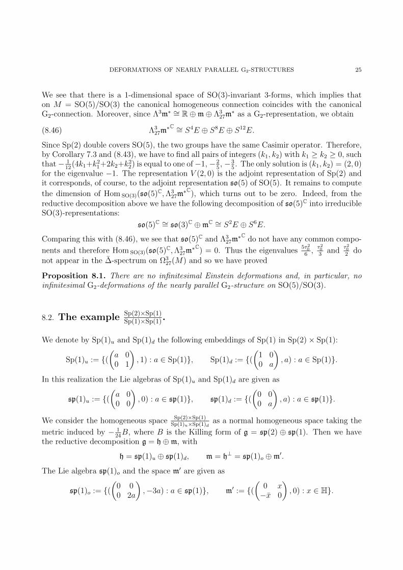
DEFORMATIONS OF NEARLY PARALLEL G2-STRUCTURES 25
We see that there is a 1-dimensional space of SO(3)-invariant 3-forms, which implies thaton M = SO(5)/SO(3) the canonical homogeneous connection coincides with the canonicalG2-connection. Moreover, since Λ3m∗ ∼= R⊕m⊕ Λ3
27m∗ as a G2-representation, we obtain
(8.46) Λ327m
∗C ∼= S4E ⊕ S8E ⊕ S12E.
Since Sp(2) double covers SO(5), the two groups have the same Casimir operator. Therefore,by Corollary 7.3 and (8.43), we have to find all pairs of integers (k1, k2) with k1 ≥ k2 ≥ 0, suchthat− 1
12(4k1+k2
1+2k2+k22) is equal to one of−1, −2
5, −3
5. The only solution is (k1, k2) = (2, 0)
for the eigenvalue −1. The representation V (2, 0) is the adjoint representation of Sp(2) andit corresponds, of course, to the adjoint representation so(5) of SO(5). It remains to compute
the dimension of Hom SO(3)(so(5)C,Λ327m
∗C), which turns out to be zero. Indeed, from thereductive decomposition above we have the following decomposition of so(5)C into irreducibleSO(3)-representations:
so(5)C ∼= so(3)C ⊕mC ∼= S2E ⊕ S6E.
Comparing this with (8.46), we see that so(5)C and Λ327m
∗C do not have any common compo-
nents and therefore Hom SO(3)(so(5)C,Λ327m
∗C) = 0. Thus the eigenvalues5τ206
,τ203
andτ202
donot appear in the ∆-spectrum on Ω3
27(M) and so we have proved
Proposition 8.1. There are no infinitesimal Einstein deformations and, in particular, noinfinitesimal G2-deformations of the nearly parallel G2-structure on SO(5)/SO(3).
8.2. The example Sp(2)×Sp(1)Sp(1)×Sp(1).
We denote by Sp(1)u and Sp(1)d the following embeddings of Sp(1) in Sp(2)× Sp(1):
Sp(1)u := ((a 00 1
), 1) : a ∈ Sp(1), Sp(1)d := (
(1 00 a
), a) : a ∈ Sp(1).
In this realization the Lie algebras of Sp(1)u and Sp(1)d are given as
sp(1)u := ((a 00 0
), 0) : a ∈ sp(1), sp(1)d := (
(0 00 a
), a) : a ∈ sp(1).
We consider the homogeneous space Sp(2)×Sp(1)Sp(1)u×Sp(1)d
as a normal homogeneous space taking the
metric induced by − 124B, where B is the Killing form of g = sp(2) ⊕ sp(1). Then we have
the reductive decomposition g = h⊕m, with
h = sp(1)u ⊕ sp(1)d, m = h⊥ = sp(1)o ⊕m′.
The Lie algebra sp(1)o and the space m′ are given as
sp(1)o := ((
0 00 2a
),−3a) : a ∈ sp(1), m′ := (
(0 x−x 0
), 0) : x ∈ H.
26 B. ALEXANDROV, U. SEMMELMANN
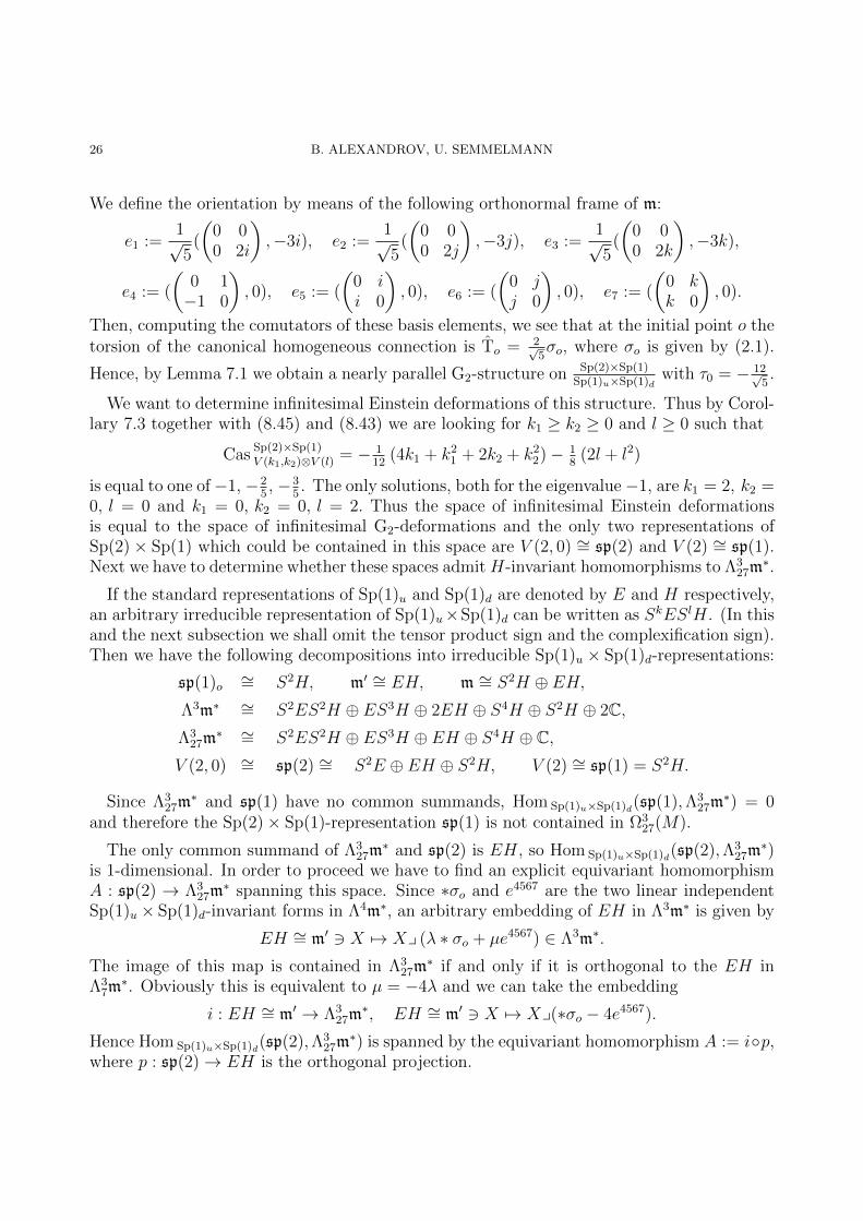
We define the orientation by means of the following orthonormal frame of m:
e1 :=1√5
(
(0 00 2i
),−3i), e2 :=
1√5
(
(0 00 2j
),−3j), e3 :=
1√5
(
(0 00 2k
),−3k),
e4 := (
(0 1−1 0
), 0), e5 := (
(0 ii 0
), 0), e6 := (
(0 jj 0
), 0), e7 := (
(0 kk 0
), 0).
Then, computing the comutators of these basis elements, we see that at the initial point o thetorsion of the canonical homogeneous connection is To = 2√
5σo, where σo is given by (2.1).
Hence, by Lemma 7.1 we obtain a nearly parallel G2-structure on Sp(2)×Sp(1)Sp(1)u×Sp(1)d
with τ0 = − 12√5.
We want to determine infinitesimal Einstein deformations of this structure. Thus by Corol-lary 7.3 together with (8.45) and (8.43) we are looking for k1 ≥ k2 ≥ 0 and l ≥ 0 such that
CasSp(2)×Sp(1)V (k1,k2)⊗V (l) = − 1
12(4k1 + k2
1 + 2k2 + k22)− 1
8(2l + l2)
is equal to one of−1, −25, −3
5. The only solutions, both for the eigenvalue−1, are k1 = 2, k2 =
0, l = 0 and k1 = 0, k2 = 0, l = 2. Thus the space of infinitesimal Einstein deformationsis equal to the space of infinitesimal G2-deformations and the only two representations ofSp(2)× Sp(1) which could be contained in this space are V (2, 0) ∼= sp(2) and V (2) ∼= sp(1).Next we have to determine whether these spaces admit H-invariant homomorphisms to Λ3
27m∗.
If the standard representations of Sp(1)u and Sp(1)d are denoted by E and H respectively,an arbitrary irreducible representation of Sp(1)u×Sp(1)d can be written as SkESlH. (In thisand the next subsection we shall omit the tensor product sign and the complexification sign).Then we have the following decompositions into irreducible Sp(1)u × Sp(1)d-representations:
sp(1)o ∼= S2H, m′ ∼= EH, m ∼= S2H ⊕ EH,Λ3m∗ ∼= S2ES2H ⊕ ES3H ⊕ 2EH ⊕ S4H ⊕ S2H ⊕ 2C,Λ3
27m∗ ∼= S2ES2H ⊕ ES3H ⊕ EH ⊕ S4H ⊕ C,
V (2, 0) ∼= sp(2) ∼= S2E ⊕ EH ⊕ S2H, V (2) ∼= sp(1) = S2H.
Since Λ327m
∗ and sp(1) have no common summands, Hom Sp(1)u×Sp(1)d(sp(1),Λ327m
∗) = 0and therefore the Sp(2)× Sp(1)-representation sp(1) is not contained in Ω3
27(M).
The only common summand of Λ327m
∗ and sp(2) is EH, so Hom Sp(1)u×Sp(1)d(sp(2),Λ327m
∗)is 1-dimensional. In order to proceed we have to find an explicit equivariant homomorphismA : sp(2) → Λ3
27m∗ spanning this space. Since ∗σo and e4567 are the two linear independent
Sp(1)u × Sp(1)d-invariant forms in Λ4m∗, an arbitrary embedding of EH in Λ3m∗ is given by
EH ∼= m′ 3 X 7→ Xy (λ ∗ σo + µe4567) ∈ Λ3m∗.
The image of this map is contained in Λ327m
∗ if and only if it is orthogonal to the EH inΛ3
7m∗. Obviously this is equivalent to µ = −4λ and we can take the embedding
i : EH ∼= m′ → Λ327m
∗, EH ∼= m′ 3 X 7→ Xy(∗σo − 4e4567).
Hence Hom Sp(1)u×Sp(1)d(sp(2),Λ327m
∗) is spanned by the equivariant homomorphism A := ip,where p : sp(2)→ EH is the orthogonal projection.
DEFORMATIONS OF NEARLY PARALLEL G2-STRUCTURES 27
Thus U = sp(2) is the only Sp(2) × Sp(1)-representation which remains for the solutionspace of the equation ∗dϕ = −τ0ϕ, describing the infinitesimal G2-deformations. As men-tioned above, this equation is equivalent to (d + 5
6τ0∗)ϕ = 0, i.e. in the case at hand to
(d−2√
5∗)ϕ = 0. From the results of the last part of Section 7 for V = Λ327m
∗ and U = sp(2)it follows that equation (7.42) with c = −2
√5 must be satisfied for the chosen A and all
u ∈ sp(2). However this is not the case: take α := e4 ∈ EH ∼= m′ ⊂ sp(2). Then
e1 · α = [e1, e4] = − 2√5e5, i(e5) = 3e467 + e137 + e126 + e234,
e2 · α = [e2, e4] = − 2√5e6, i(e6) = −3e457 + e237 − e125 − e134,
e3 · α = [e3, e4] = − 2√5e7, i(e7) = 3e456 − e236 − e135 + e124,
e4 · α = [e4, e4] = 0, i(e4) = −3e567 − e235 + e136 − e127.
Using these equations one easily sees that the coefficient of e1234 in the left-hand side of (7.42)is 36√
56= 0. Hence sp(2) is not contained in the space of solutions of (d− 2
√5∗)ϕ = 0.
Since the nearly parallel G2-structure of the squashed sphere is a double covering of theone on RP 7 the same argument applies for the real projective space and we obtain
Proposition 8.2. There are no infinitesimal Einstein deformations and, in particular, no in-
finitesimal G2-deformations of the nearly parallel G2-structure on the squashed sphere Sp(2)×Sp(1)Sp(1)×Sp(1)
and of the nearly parallel G2-structure on RP 7 inducing the second Einstein metric.
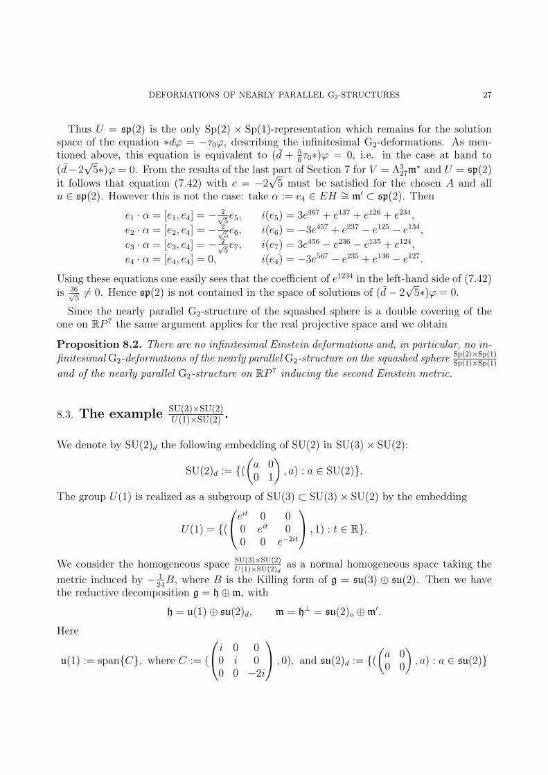
8.3. The example SU(3)×SU(2)U(1)×SU(2) .
We denote by SU(2)d the following embedding of SU(2) in SU(3)× SU(2):
SU(2)d := ((a 00 1
), a) : a ∈ SU(2).
The group U(1) is realized as a subgroup of SU(3) ⊂ SU(3)× SU(2) by the embedding
U(1) = (
eit 0 00 eit 00 0 e−2it
, 1) : t ∈ R.
We consider the homogeneous space SU(3)×SU(2)U(1)×SU(2)d
as a normal homogeneous space taking the
metric induced by − 124B, where B is the Killing form of g = su(3) ⊕ su(2). Then we have
the reductive decomposition g = h⊕m, with
h = u(1)⊕ su(2)d, m = h⊥ = su(2)o ⊕m′.
Here
u(1) := spanC, where C := (
i 0 00 i 00 0 −2i
, 0), and su(2)d := ((a 00 0
), a) : a ∈ su(2)
28 B. ALEXANDROV, U. SEMMELMANN
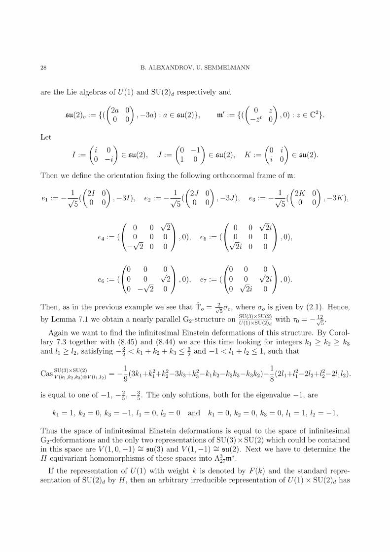
are the Lie algebras of U(1) and SU(2)d respectively and
su(2)o := ((
2a 00 0
),−3a) : a ∈ su(2), m′ := (
(0 z−zt 0
), 0) : z ∈ C2.
Let
I :=
(i 00 −i
)∈ su(2), J :=
(0 −11 0
)∈ su(2), K :=
(0 ii 0
)∈ su(2).
Then we define the orientation fixing the following orthonormal frame of m:
e1 := − 1√5
(
(2I 00 0
),−3I), e2 := − 1√
5(
(2J 00 0
),−3J), e3 := − 1√
5(
(2K 00 0
),−3K),
e4 := (
0 0√
20 0 0
−√
2 0 0
, 0), e5 := (
0 0√
2i0 0 0√2i 0 0
, 0),
e6 := (
0 0 0
0 0√
2
0 −√
2 0
, 0), e7 := (
0 0 0
0 0√
2i
0√
2i 0
, 0).
Then, as in the previous example we see that To = 2√5σo, where σo is given by (2.1). Hence,
by Lemma 7.1 we obtain a nearly parallel G2-structure on SU(3)×SU(2)U(1)×SU(2)d
with τ0 = − 12√5.
Again we want to find the infinitesimal Einstein deformations of this structure. By Corol-lary 7.3 together with (8.45) and (8.44) we are this time looking for integers k1 ≥ k2 ≥ k3
and l1 ≥ l2, satisfying −32< k1 + k2 + k3 ≤ 3
2and −1 < l1 + l2 ≤ 1, such that
CasSU(3)×SU(2)V (k1,k2,k3)⊗V (l1,l2) = −1
9(3k1+k2
1+k22−3k3+k2
3−k1k2−k2k3−k3k2)−1
8(2l1+l21−2l2+l22−2l1l2).
is equal to one of −1, −25, −3
5. The only solutions, both for the eigenvalue −1, are
k1 = 1, k2 = 0, k3 = −1, l1 = 0, l2 = 0 and k1 = 0, k2 = 0, k3 = 0, l1 = 1, l2 = −1,
Thus the space of infinitesimal Einstein deformations is equal to the space of infinitesimalG2-deformations and the only two representations of SU(3)×SU(2) which could be containedin this space are V (1, 0,−1) ∼= su(3) and V (1,−1) ∼= su(2). Next we have to determine theH-equivariant homomorphisms of these spaces into Λ3
27m∗.
If the representation of U(1) with weight k is denoted by F (k) and the standard repre-sentation of SU(2)d by H, then an arbitrary irreducible representation of U(1)× SU(2)d has
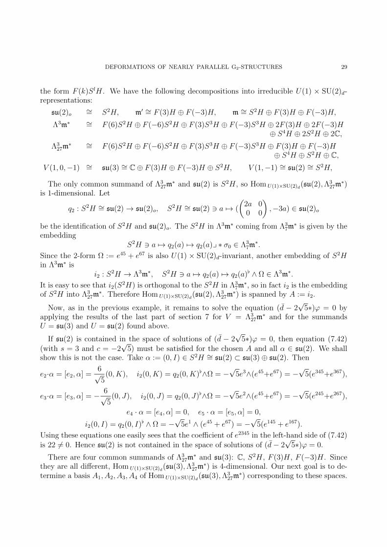
DEFORMATIONS OF NEARLY PARALLEL G2-STRUCTURES 29
the form F (k)SlH. We have the following decompositions into irreducible U(1) × SU(2)d-representations:
su(2)o ∼= S2H, m′ ∼= F (3)H ⊕ F (−3)H, m ∼= S2H ⊕ F (3)H ⊕ F (−3)H,
Λ3m∗ ∼= F (6)S2H ⊕ F (−6)S2H ⊕ F (3)S3H ⊕ F (−3)S3H ⊕ 2F (3)H ⊕ 2F (−3)H⊕ S4H ⊕ 2S2H ⊕ 2C,
Λ327m
∗ ∼= F (6)S2H ⊕ F (−6)S2H ⊕ F (3)S3H ⊕ F (−3)S3H ⊕ F (3)H ⊕ F (−3)H⊕ S4H ⊕ S2H ⊕ C,
V (1, 0,−1) ∼= su(3) ∼= C⊕ F (3)H ⊕ F (−3)H ⊕ S2H, V (1,−1) ∼= su(2) ∼= S2H,
The only common summand of Λ327m
∗ and su(2) is S2H, so Hom U(1)×SU(2)d(su(2),Λ327m
∗)is 1-dimensional. Let
q2 : S2H ∼= su(2)→ su(2)o, S2H ∼= su(2) 3 a 7→ (
(2a 00 0
),−3a) ∈ su(2)o
be the identification of S2H and su(2)o. The S2H in Λ3m∗ coming from Λ37m∗ is given by the
embeddingS2H 3 a 7→ q2(a) 7→ q2(a)y ∗ σ0 ∈ Λ3
7m∗.
Since the 2-form Ω := e45 + e67 is also U(1) × SU(2)d-invariant, another embedding of S2Hin Λ3m∗ is
i2 : S2H → Λ3m∗, S2H 3 a 7→ q2(a) 7→ q2(a)[ ∧ Ω ∈ Λ3m∗.
It is easy to see that i2(S2H) is orthogonal to the S2H in Λ37m∗, so in fact i2 is the embedding
of S2H into Λ327m
∗. Therefore Hom U(1)×SU(2)d(su(2),Λ327m
∗) is spanned by A := i2.
Now, as in the previous example, it remains to solve the equation (d − 2√
5∗)ϕ = 0 byapplying the results of the last part of section 7 for V = Λ3
27m∗ and for the summands
U = su(3) and U = su(2) found above.
If su(2) is contained in the space of solutions of (d − 2√
5∗)ϕ = 0, then equation (7.42)(with s = 3 and c = −2
√5) must be satisfied for the chosen A and all α ∈ su(2). We shall
show this is not the case. Take α := (0, I) ∈ S2H ∼= su(2) ⊂ su(3)⊕ su(2). Then
e2·α = [e2, α] =6√5
(0, K), i2(0, K) = q2(0, K)[∧Ω = −√
5e3∧(e45+e67) = −√
5(e345+e367),
e3·α = [e3, α] = − 6√5
(0, J), i2(0, J) = q2(0, J)[∧Ω = −√
5e2∧(e45+e67) = −√
5(e245+e267),
e4 · α = [e4, α] = 0, e5 · α = [e5, α] = 0,
i2(0, I) = q2(0, I)[ ∧ Ω = −√
5e1 ∧ (e45 + e67) = −√
5(e145 + e167).
Using these equations one easily sees that the coefficient of e2345 in the left-hand side of (7.42)is 22 6= 0. Hence su(2) is not contained in the space of solutions of (d− 2
√5∗)ϕ = 0.
There are four common summands of Λ327m
∗ and su(3): C, S2H, F (3)H, F (−3)H. Sincethey are all different, Hom U(1)×SU(2)d(su(3),Λ3
27m∗) is 4-dimensional. Our next goal is to de-
termine a basis A1, A2, A3, A4 of Hom U(1)×SU(2)d(su(3),Λ327m
∗) corresponding to these spaces.
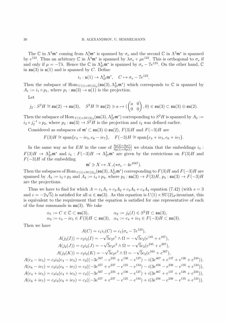
30 B. ALEXANDROV, U. SEMMELMANN
The C in Λ3m∗ coming from Λ31m∗ is spanned by σo and the second C in Λ3m∗ is spanned
by e123. Thus an arbitrary C in Λ3m∗ is spanned by λσo + µe123. This is orthogonal to σo ifand only if µ = −7λ. Hence the C in Λ3
27m∗ is spanned by σo − 7e123. On the other hand, C
in su(3) is u(1) and is spanned by C. Define
i1 : u(1)→ Λ327m
∗, C 7→ σo − 7e123.
Then the subspace of Hom U(1)×SU(2)d(su(3),Λ327m
∗) which corresponds to C is spanned byA1 := i1 p1, where p1 : su(3)→ u(1) is the projection.
Let
j2 : S2H ∼= su(2)→ su(3), S2H ∼= su(2) 3 a 7→ (
(a 00 0
), 0) ∈ su(3) ⊂ su(3)⊕ su(2).
Then the subspace of Hom U(1)×SU(2)d(su(3),Λ327m
∗) corresponding to S2H is spanned by A2 :=i2 j−1
2 p2, where p2 : su(3)→ S2H is the projection and i2 was defined earlier.
Considered as subspaces of m′ ⊂ su(3)⊕ su(2), F (3)H and F (−3)H are
F (3)H ∼= spane4 − ie5, e6 − ie7, F (−3)H ∼= spane4 + ie5, e6 + ie7.
In the same way as for EH in the case of Sp(2)×Sp(1)Sp(1)×Sp(1)
we obtain that the embeddings i3 :
F (3)H → Λ327m
∗ and i4 : F (−3)H → Λ327m
∗ are given by the restrictions on F (3)H andF (−3)H of the embedding
m′ 3 X 7→ Xy(∗σo − 4e4567).
Then the subspaces of Hom U(1)×SU(2)d(su(3),Λ327m
∗) corresponding to F (3)H and F (−3)H arespanned by A3 := i3 p3 and A4 := i4 p4, where p3 : su(3)→ F (3)H, p4 : su(3)→ F (−3)Hare the projections.
Thus we have to find for which A = c1A1 + c2A2 + c3A3 + c4A4 equation (7.42) (with s = 3and c = −2
√5) is satisfied for all α ∈ su(3). As this equation is U(1)×SU(2)d-invariant, this
is equivalent to the requirement that the equation is satisfied for one representative of eachof the four summands in su(3). We take
α1 := C ∈ C ⊂ su(3), α2 := j2(I) ∈ S2H ⊂ su(3),α3 := e4 − ie5 ∈ F (3)H ⊂ su(3), α4 := e4 + ie5 ∈ F (−3)H ⊂ su(3).
Then we haveA(C) = c1i1(C) = c1(σo − 7e123),
A(j2(I)) = c2i2(I) = −√
5c2e1 ∧ Ω = −
√5c2(e145 + e167),
A(j2(J)) = c2i2(J) = −√
5c2e2 ∧ Ω = −
√5c2(e245 + e267),
A(j2(K)) = c2i2(K) = −√
5c2e3 ∧ Ω = −
√5c2(e345 + e367),
A(e4 − ie5) = c3i3(e4 − ie5) = c3((−3e567 − e235 + e136 − e127)− i(3e467 + e137 + e126 + e234)),
A(e6 − ie7) = c3i3(e6 − ie7) = c3((−3e457 + e237 − e125 − e134)− i(3e456 − e236 − e135 + e124)),
A(e4 + ie5) = c4i4(e4 + ie5) = c4((−3e567 − e235 + e136 − e127) + i(3e467 + e137 + e126 + e234)),
A(e6 + ie7) = c4i4(e6 + ie7) = c4((−3e457 + e237 − e125 − e134) + i(3e456 − e236 − e135 + e124)).
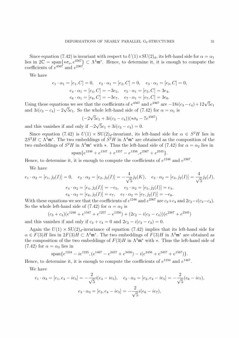
DEFORMATIONS OF NEARLY PARALLEL G2-STRUCTURES 31
Since equation (7.42) is invariant with respect to U(1)×SU(2)d, its left-hand side for α = α1
lies in 2C = span∗σo, e4567 ⊂ Λ4m∗. Hence, to determine it, it is enough to compute thecoefficients of e4567 and e2367.
We have
e1 · α1 = [e1, C] = 0, e2 · α1 = [e2, C] = 0, e3 · α1 = [e3, C] = 0,
e4 · α1 = [e4, C] = −3e5, e5 · α1 = [e5, C] = 3e4,
e6 · α1 = [e6, C] = −3e7, e7 · α1 = [e7, C] = 3e6.
Using these equations we see that the coefficients of e4567 and e2367 are −18i(c3−c4)+12√
5c1
and 3i(c3 − c4)− 2√
5c1. So the whole left-hand side of (7.42) for α = α1 is
(−2√
5c1 + 3i(c3 − c4))(∗σ0 − 7e4567)
and this vanishes if and only if −2√
5c1 + 3i(c3 − c4) = 0.
Since equation (7.42) is U(1) × SU(2)d-invariant, its left-hand side for α ∈ S2H lies in2S2H ⊂ Λ4m∗. The two embeddings of S2H in Λ4m∗ are obtained as the composition of thetwo embeddings of S2H in Λ3m∗ with ∗. Thus the left-hand side of (7.42) for α = α2 lies in
spane1246 + e1347 + e1257 − e1356, e2367 + e2345.Hence, to determine it, it is enough to compute the coefficients of e1246 and e2367.
We have
e1 · α2 = [e1, j2(I)] = 0, e2 · α2 = [e2, j2(I)] = − 4√5j2(K), e3 · α2 = [e3, j2(I)] =
4√5j2(J),
e4 · α2 = [e4, j2(I)] = −e5, e5 · α2 = [e5, j2(I)] = e4,
e6 · α2 = [e6, j2(I)] = e7, e7 · α2 = [e7, j2(I)] = −e6.
With these equations we see that the coefficients of e1246 and e2367 are c3+c4 and 2c2−i(c3−c4).So the whole left-hand side of (7.42) for α = α2 is
(c3 + c4)(e1246 + e1347 + e1257 − e1356) + (2c2 − i(c3 − c4))(e2367 + e2345)
and this vanishes if and only if c3 + c4 = 0 and 2c2 − i(c3 − c4) = 0.
Again the U(1) × SU(2)d-invariance of equation (7.42) implies that its left-hand side forα ∈ F (3)H lies in 2F (3)H ⊂ Λ4m∗. The two embeddings of F (3)H in Λ4m∗ are obtained asthe composition of the two embeddings of F (3)H in Λ3m∗ with ∗. Thus the left-hand side of(7.42) for α = α3 lies in
spane1234 − ie1235, (e1467 − e2457 + e3456)− i(e2456 + e3457 + e1567).Hence, to determine it, it is enough to compute the coefficients of e1234 and e1467.
We have
e1 · α3 = [e1, e4 − ie5] = − 2√5i(e4 − ie5), e2 · α3 = [e2, e4 − ie5] = − 2√
5(e6 − ie7),
e3 · α3 = [e3, e4 − ie5] = − 2√5i(e6 − ie7),
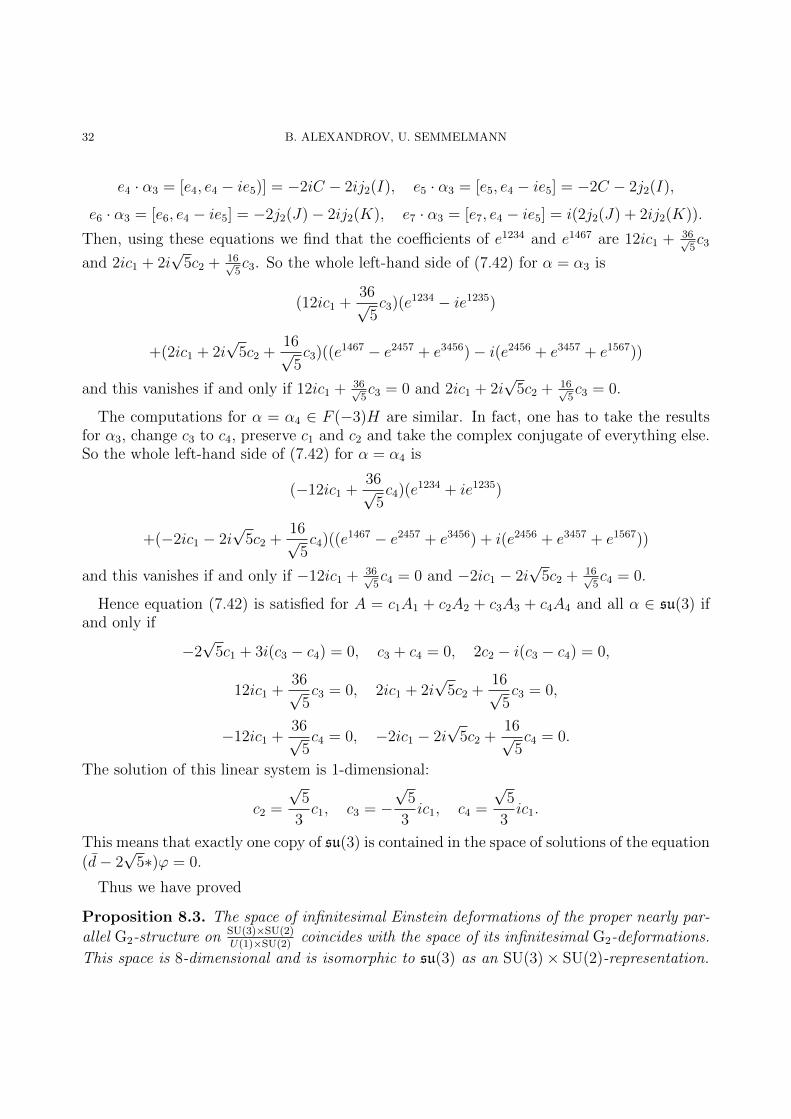
32 B. ALEXANDROV, U. SEMMELMANN
e4 · α3 = [e4, e4 − ie5)] = −2iC − 2ij2(I), e5 · α3 = [e5, e4 − ie5] = −2C − 2j2(I),
e6 · α3 = [e6, e4 − ie5] = −2j2(J)− 2ij2(K), e7 · α3 = [e7, e4 − ie5] = i(2j2(J) + 2ij2(K)).
Then, using these equations we find that the coefficients of e1234 and e1467 are 12ic1 + 36√5c3
and 2ic1 + 2i√
5c2 + 16√5c3. So the whole left-hand side of (7.42) for α = α3 is
(12ic1 +36√
5c3)(e1234 − ie1235)
+(2ic1 + 2i√
5c2 +16√
5c3)((e1467 − e2457 + e3456)− i(e2456 + e3457 + e1567))
and this vanishes if and only if 12ic1 + 36√5c3 = 0 and 2ic1 + 2i
√5c2 + 16√
5c3 = 0.
The computations for α = α4 ∈ F (−3)H are similar. In fact, one has to take the resultsfor α3, change c3 to c4, preserve c1 and c2 and take the complex conjugate of everything else.So the whole left-hand side of (7.42) for α = α4 is
(−12ic1 +36√
5c4)(e1234 + ie1235)
+(−2ic1 − 2i√
5c2 +16√
5c4)((e1467 − e2457 + e3456) + i(e2456 + e3457 + e1567))
and this vanishes if and only if −12ic1 + 36√5c4 = 0 and −2ic1 − 2i
√5c2 + 16√
5c4 = 0.
Hence equation (7.42) is satisfied for A = c1A1 + c2A2 + c3A3 + c4A4 and all α ∈ su(3) ifand only if
−2√
5c1 + 3i(c3 − c4) = 0, c3 + c4 = 0, 2c2 − i(c3 − c4) = 0,
12ic1 +36√
5c3 = 0, 2ic1 + 2i
√5c2 +
16√5c3 = 0,
−12ic1 +36√
5c4 = 0, −2ic1 − 2i
√5c2 +
16√5c4 = 0.
The solution of this linear system is 1-dimensional:
c2 =
√5
3c1, c3 = −
√5
3ic1, c4 =
√5
3ic1.
This means that exactly one copy of su(3) is contained in the space of solutions of the equation(d− 2
√5∗)ϕ = 0.
Thus we have proved
Proposition 8.3. The space of infinitesimal Einstein deformations of the proper nearly par-
allel G2-structure on SU(3)×SU(2)U(1)×SU(2)
coincides with the space of its infinitesimal G2-deformations.
This space is 8-dimensional and is isomorphic to su(3) as an SU(3)× SU(2)-representation.
DEFORMATIONS OF NEARLY PARALLEL G2-STRUCTURES 33
References
[1] B. Alexandrov, 3-Sasakian manifolds and intrinsic torsion, to appear.[2] C. Bar, Real Killing spinors and holonomy, Commun. Math. Phys. 154 (1993), 509–521.[3] A. Besse, Einstein manifolds, Ergebnisse der Mathematik und ihrer Grenzgebiete (3) 10. Springer-Verlag,
Berlin, 1987.[4] C. Boyer, K. Galicki, Sasakian geometry, Oxford Mathematical Monographs, Oxford University Press,
Oxford, 2008.[5] R. Bryant, Metrics with exceptional holonomy, Ann. Math. 126 (1987), 525–576.[6] R. Bryant, Some remarks on G2-structures, Proceedings of Gokova Geometry-Topology Conference 2005,
75–109, Gokova Geometry/Topology Conference (GGT), Gokova, 2006. arXiv:math/0305124[7] R. Cleyton, A. Swann, Einstein metrics via intrinsic or parallel torsion, Math. Z. 247 (2004), no. 3,
513–528.[8] M. Fernandez, A. Gray, Riemannian manifolds with structure group G2, Ann. Mat. Pura Appl. (4) 132
(1982), 19–45 (1983).[9] Th. Friedrich, Nearly Kahler and nearly parallel G2-structures on spheres, Arch. Math. Brno 42 (2006),
Supplement, 241–243.[10] Th. Friedrich, S. Ivanov, Parallel spinors and connections with skew-symmetric torsion in string theory,
Asian J. Math. 6 (2002), no. 2, 303–336.[11] Th. Friedrich, I. Kath, 7-dimensional compact Riemannian manifolds with Killing spinors, Commun.
Math. Phys. 133 (1990), 543–561.[12] Th. Friedrich, I. Kath, A. Moroianu, U. Semmelmann, On nearly parallel G2-structures, J. Geom. Phys.
23 (1997), no. 3-4, 259–286.[13] A. Gray, Vector cross products on manifolds, Trans. Amer. Math. Soc. 141 (1969), 463–504. Correction,
148 (1970), 69-75.[14] D. Joyce, Compact manifolds with special holonomy, Oxford Mathematical Monographs, Oxford Univer-
sity Press, Oxford, 2000.[15] S. Kobayashi, Transformation groups in differential geometry, Ergebnisse der Mathematik und ihrer
Grenzgebiete, Springer-Verlag, Berlin-Heidelberg-New York, 1972.[16] A. Moroianu, P-A. Nagy, U. Semmelmann, Deformations of nearly Kahler structures, Pacific J. Math.
235 (2008), no. 1, 57–72.[17] A. Moroianu, U. Semmelmann, Parallel Spinors and holonomy groups, J. Math. Phys. 41 (2000), 2395-
2402.[18] A. Moroianu, U. Semmelmann, Infinitesimal Einstein Deformations of Nearly Kahler Metrics, Pacific J.
Math. 235 (2008), 57-72.[19] A. Moroianu, U. Semmelmann, The Hermitian Laplace Operator on Nearly Kahler Manifolds, Commun.
Math. Phys. 294 (2010), 251-272.[20] U. Semmelmann, Conformal Killing forms on Riemannian manifolds, Math. Z. 245 (2003), no. 3, 503–
527.[21] M. Wang, On non-simply connected manifolds with non-trivial parallel spinors, Ann. Global Anal. Geom.
13 (1995), 31–42.[22] B. Wilking, The normal homogeneous space (SU(3)×SO(3))/U•(2) has positive sectional curvature, Proc.
Amer. Math. Soc. 127 (1999), no. 4, 1191–1194.
Bogdan Alexandrov, Faculty of Mathematics and Informatics, University of Sofia ’St.Kliment Ohridski’, James Bourchier Blvd. 5, 1164 Sofia, Bulgaria
E-mail address: [email protected]
34 B. ALEXANDROV, U. SEMMELMANN
Uwe Semmelmann, Institut fur Geometrie und Topologie, Fachbereich Mathematik, Uni-versitat Stuttgart, Pfaffenwaldring 57, 70569 Stuttgart, Germany
E-mail address: [email protected]