3 1 Introduction 3.1 Introduction Let gδ(

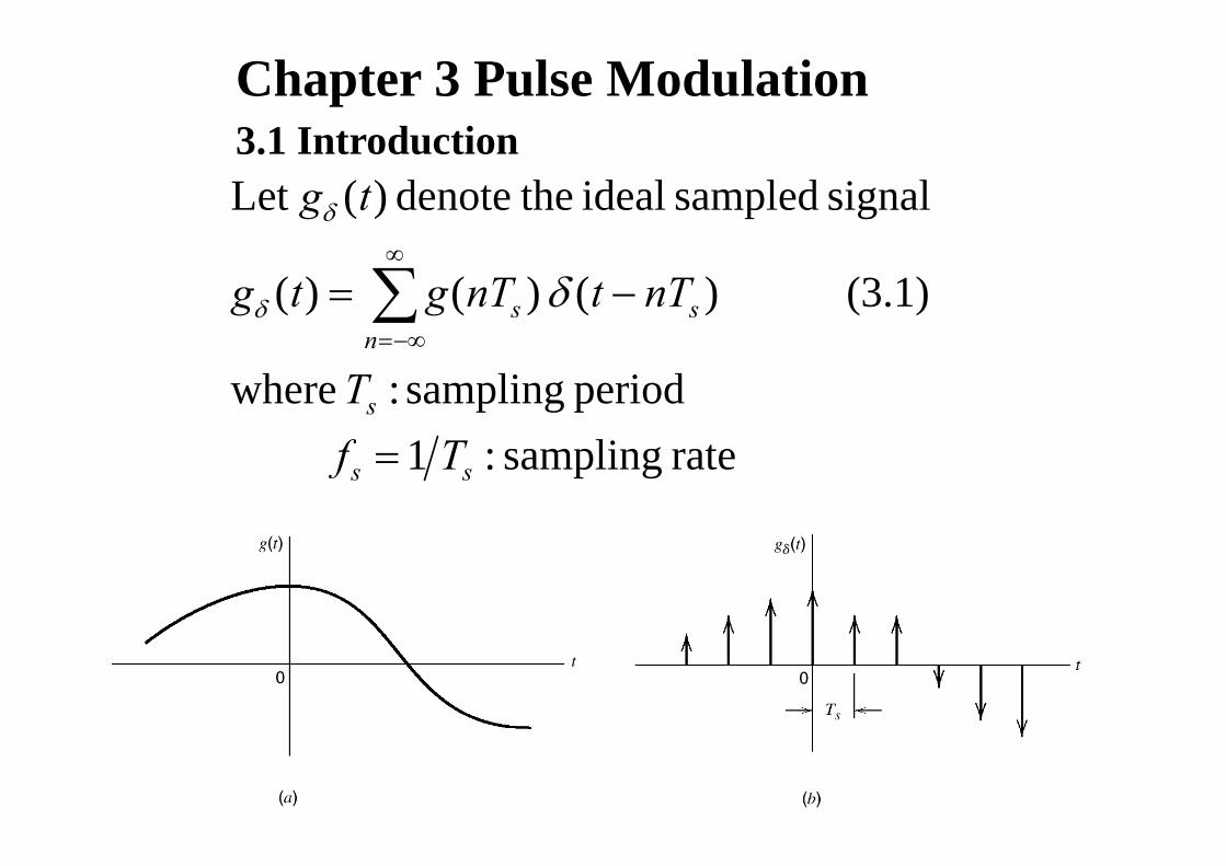
Chapter 3 Pulse Modulation3 1 Introduction

signal sampled ideal thedenote )(Let tgδ

3.1 Introduction

(3.1) )( )()( ss nTtnTgtg −= ∑∞

δδ

period sampling : where s

n

T−∞=

ratesampling:1 ss Tf =

∑∞

−∞=

⇔−n

snTtt )()g(

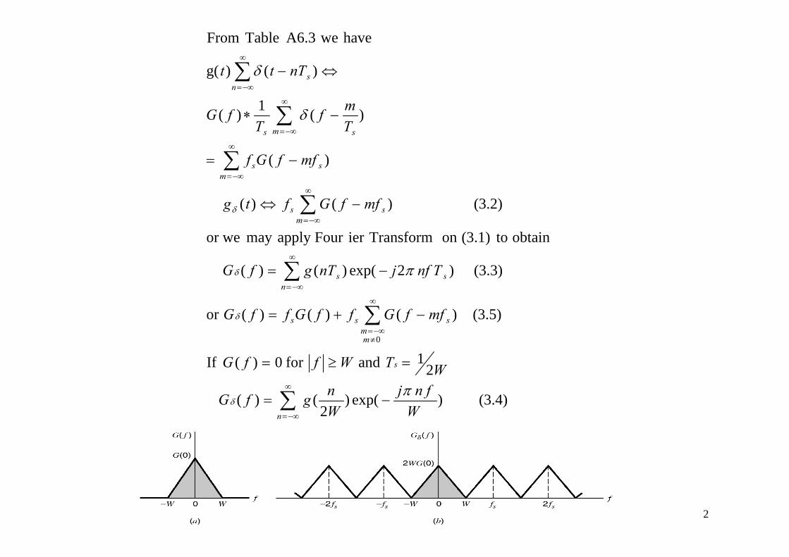
have weA6.3 Table From

δ

∑

∑∞

∞

−∞=

∞

−∗m ss

n

Tmf

TfG )(1)( δ

∑

∑∞

−∞=

−⇔

−=

ss

mss

mffGftg

mffGf

(3.2) )()(

)(

δ

∑∞

−∞=

−= ss

m

nf TjnTgfG (3.3) )2exp()()(

obtain to(3.1) on Transformier apply Fourmay or we

πδ

∑

∑∞

≠−∞=

−∞=

−+=

mm

sss

sn

s

mffGffGffG (3.5) )()()(or 0

δ

∑∞

≠

−=

=≥= s

m

n fjngfG

WTWffG

(3.4) )exp()()(

21 and for 0)( If

0

πδ ∑

−∞=n WWgf ( ))p()

2()(

2

for0)(1 With

WffG ≥

2.2for 0)(.1

WfWffG

s =

≥=

(3 6))(1)(

that (3.5) Equationfrom find we

ffGfG

as)(rewritemaywe(3 6)into(3 4)ngSubstituti

(3.6) , )(21)(

fG

WfWfGW

fG <<−= δ

(3.7),)exp()(1)(

as)(rewritemay we(3.6)into(3.4)ngSubstituti

WfWnfjngfG

fG

<<−−= ∑∞ π

for)(bydetermineduniquelyis)(

( ),)p()2

(2

)(

nngtg

fWW

gW

fn

∞<<∞−

∑−∞=

)(fi f tillt i)(

for )2

(by determineduniquely is )(

tn

nW

gtg

⎬⎫

⎨⎧

∞<<∞−

)(ofninformatioallcontains)2

(or tgW

g⎭⎬⎫

⎩⎨⎧

3

havemay we, )2

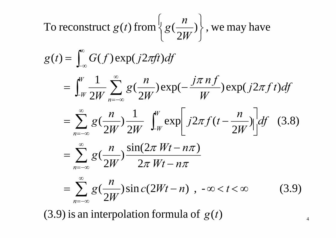
( from )(t reconstruc ToWngtg

⎭⎬⎫

⎩⎨⎧

)2exp()()(

2

dfftjfGtg

W

∫∞

∞=

⎭⎩

π

)2exp()exp()2

(21 dff tj

W n fj

Wng

WW

∫ ∑

∫∞

∞−

−= ππ

(3 8))(2e p1)(

)p()p()2

(2

dfntfjn

ffjWW

gW

W

Wn

∑ ∫

∫ ∑∞

−−∞=

⎥⎤

⎢⎡

)2sin(

(3.8) )2

(2exp 2

)2

(

nWtn

dfW

tfjWW

gn

W∑ ∫∞

−∞=− ⎥⎦

⎤⎢⎣⎡ −=

ππ

π

2

)2sin()2

( n Wt

nWtWng

n∑−∞= −

−=

ππππ

(3.9) - , )2(sin)2

( tnWtcWng∑

∞

∞

∞<<∞−=

)( offormula ioninterpolat an is (3.9)2

tgWn −∞=

4

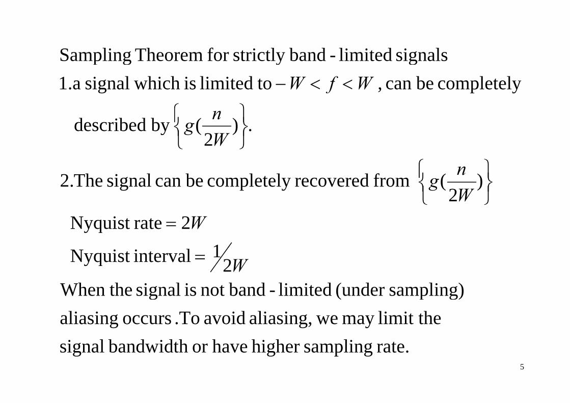
signalslimited-bandstrictly for Theorem Sampling completely be can , tolimited is whichsignal1.a

gyp gWfW

⎫⎧

<<−

.)2

(by described Wng

⎭⎬⎫

⎩⎨⎧

)2

( from recovered completely be can signal The.2Wng

⎭⎬⎫

⎩⎨⎧

12 rateNyquist W

W=

⎭⎩

sampling)(underlimited-bandnotissignaltheWhen2

1intervalNyquist W=

limit themay wealiasing, avoid .To occurs aliasingsampling)(under limitedbandnot issignal theWhen

rate.samplinghigher haveor bandwidthsignal5

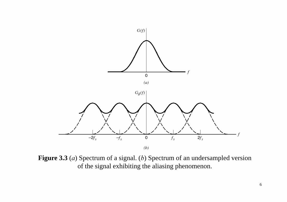
Figure 3.3 (a) Spectrum of a signal. (b) Spectrum of an undersampled version of the signal exhibiting the aliasing phenomenon.

6

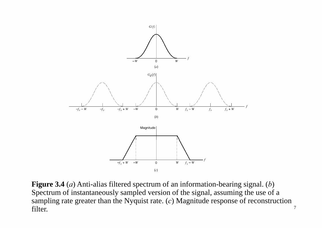
Figure 3.4 (a) Anti-alias filtered spectrum of an information-bearing signal. (b) Spectrum of instantaneously sampled version of the signal assuming the use of aSpectrum of instantaneously sampled version of the signal, assuming the use of a sampling rate greater than the Nyquist rate. (c) Magnitude response of reconstruction filter. 7

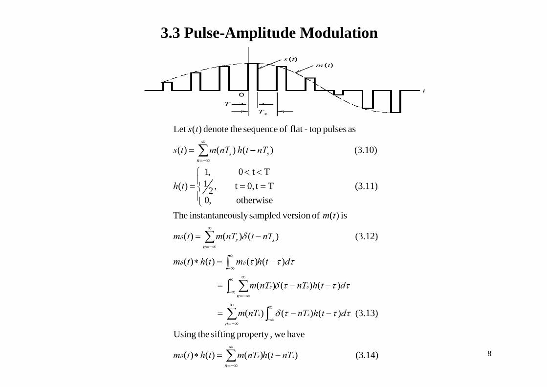
3.3 Pulse-Amplitude Modulation

(3 10))()()(

as pulses top-flat of sequence thedenote )(Let

nTthnTmts

ts

= ∑∞

(3.11) Tt0,tTt 0

,21

,1)(

(3.10) )()()( sn

s

th

nTthnTmts

⎪

⎪⎨

⎧==<<

=

−= ∑−∞=

(3 12))()()(

is )( of versionsampledously instantane Theotherwise,0

2

nTtnTmtm

tm

−=

⎪⎩

∑∞

δ δ

)()()()(

(3.12) )()()(n

ss

dthmthtm

nTtnTmtm

−=∗

=

∫ ∑

∫

∑

∞ ∞

∞

∞−

−∞=

δδ

δ

τττ

δ

(3.13) )()()(

)()()(

s

n

s

s

n

s

dthnTnTm

dthnTnTm

−−=

−−=

∫∑

∫ ∑∞

∞−

∞

−∞=

∞−−∞=

τττδ

τττδ

(3.14) )()()()(

have we,property sifting theUsing

s

n

s nTthnTmthtm −=∗ ∑∞

−∞=

δ 8

is )( signal PAM The ts

(3 16))()()((3.15) )()()(

=⇔∗=δ fHfMfS

thtmts δ

(3 2))()((3 2)R ll

(3.16) )()()(

∑∞

=⇔ δ

ffGft

fHfMfS

(3.2) )()((3.2) Recall ∑−∞=

−⇔m

ss mffGftgδ

(3.17) )()(M ∑∞

−=k

ss k ffMffδ

(3 18))()()( ∑∞

−∞=

=

k

fHk ffMffS (3.18) )()()( ∑−∞=

−=k

ss fHk ffMffS

9

與idea sampling比較多H(f)

Pulse Amplitude Modulation –Natural and Flat-Top Samplingp p g

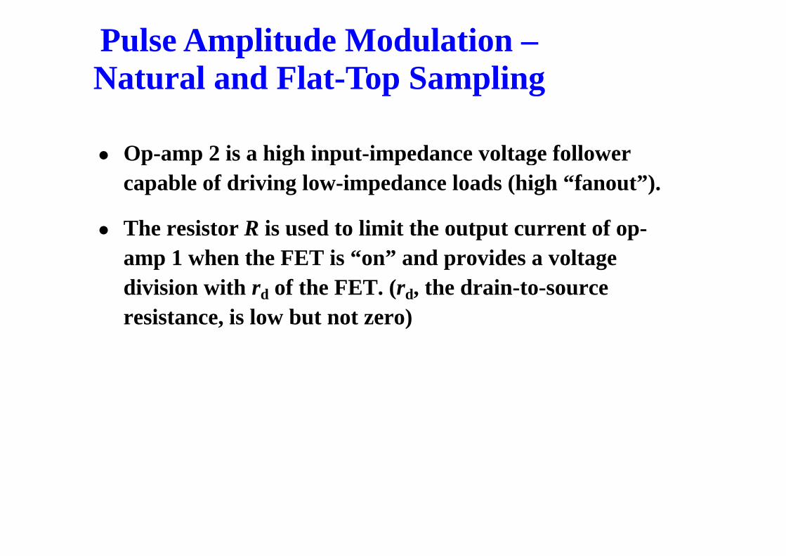
The circuit of Figure 11 3 is used to illustrate pulseThe circuit of Figure 11-3 is used to illustrate pulse amplitude modulation (PAM). The FET is the switch used as a sampling gate.p g g

When the FET is on, the analog voltage is shorted to ground; when off the FET is essentially open so thatground; when off, the FET is essentially open, so that the analog signal sample appears at the output.

O 1 i i ti lifi th t i l t thOp-amp 1 is a noninverting amplifier that isolates the analog input channel from the switching function.

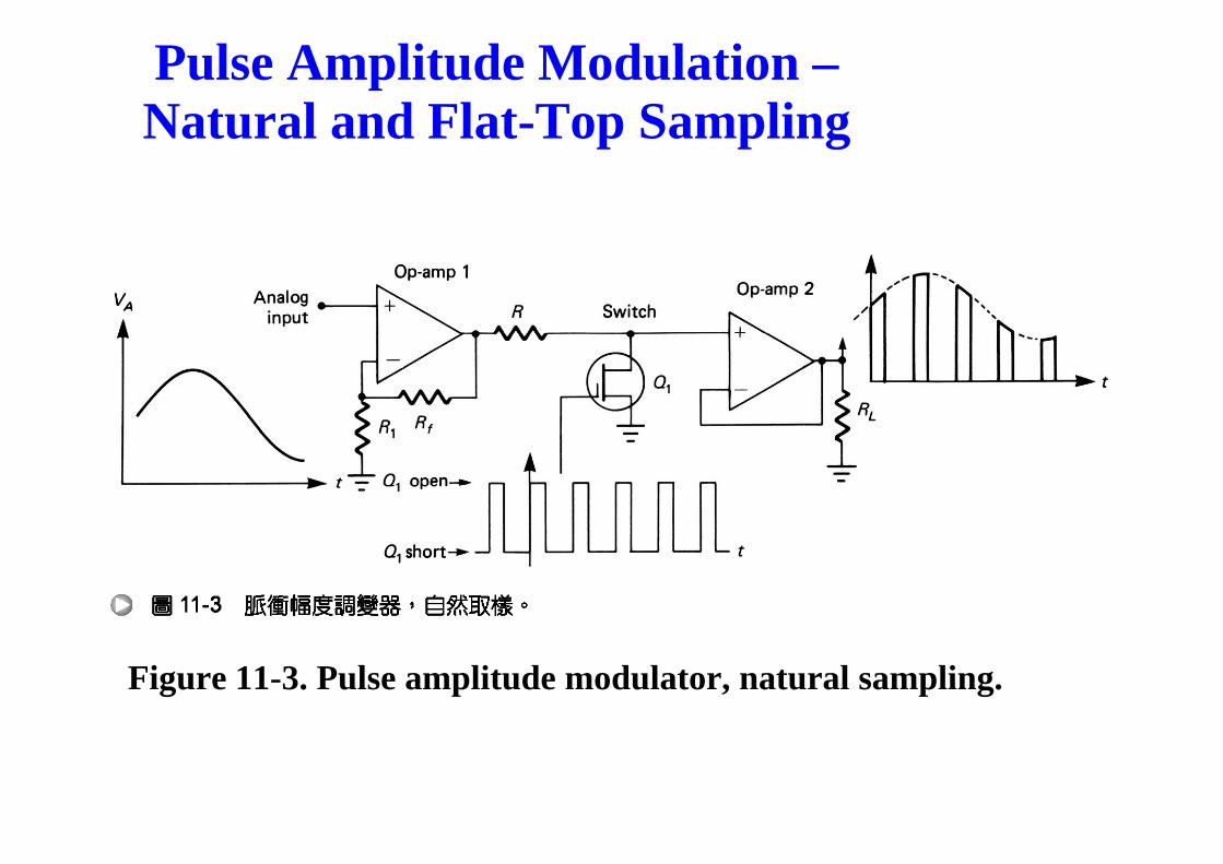
Pulse Amplitude Modulation –Natural and Flat-Top SamplingNatural and Flat Top Sampling

Figure 11-3. Pulse amplitude modulator, natural sampling.

Pulse Amplitude Modulation –Natural and Flat-Top Sampling

Op amp 2 is a high input impedance voltage follower

Natural and Flat Top Sampling

Op-amp 2 is a high input-impedance voltage follower capable of driving low-impedance loads (high “fanout”).

The resistor R is used to limit the output current of op-amp 1 when the FET is “on” and provides a voltage division with rd of the FET. (rd, the drain-to-source resistance, is low but not zero)


The most common technique for sampling voice in


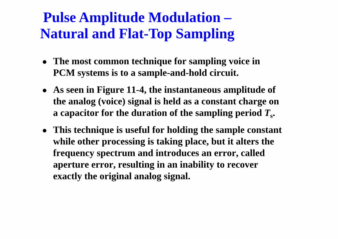
q p gPCM systems is to a sample-and-hold circuit.

As seen in Figure 11-4, the instantaneous amplitude ofAs seen in Figure 11 4, the instantaneous amplitude of the analog (voice) signal is held as a constant charge on a capacitor for the duration of the sampling period Ts.

This technique is useful for holding the sample constant while other processing is taking place, but it alters the frequency spectrum and introduces an error, called aperture error, resulting in an inability to recover

tl th i i l l i lexactly the original analog signal.


The amount of error depends on how mach the analog


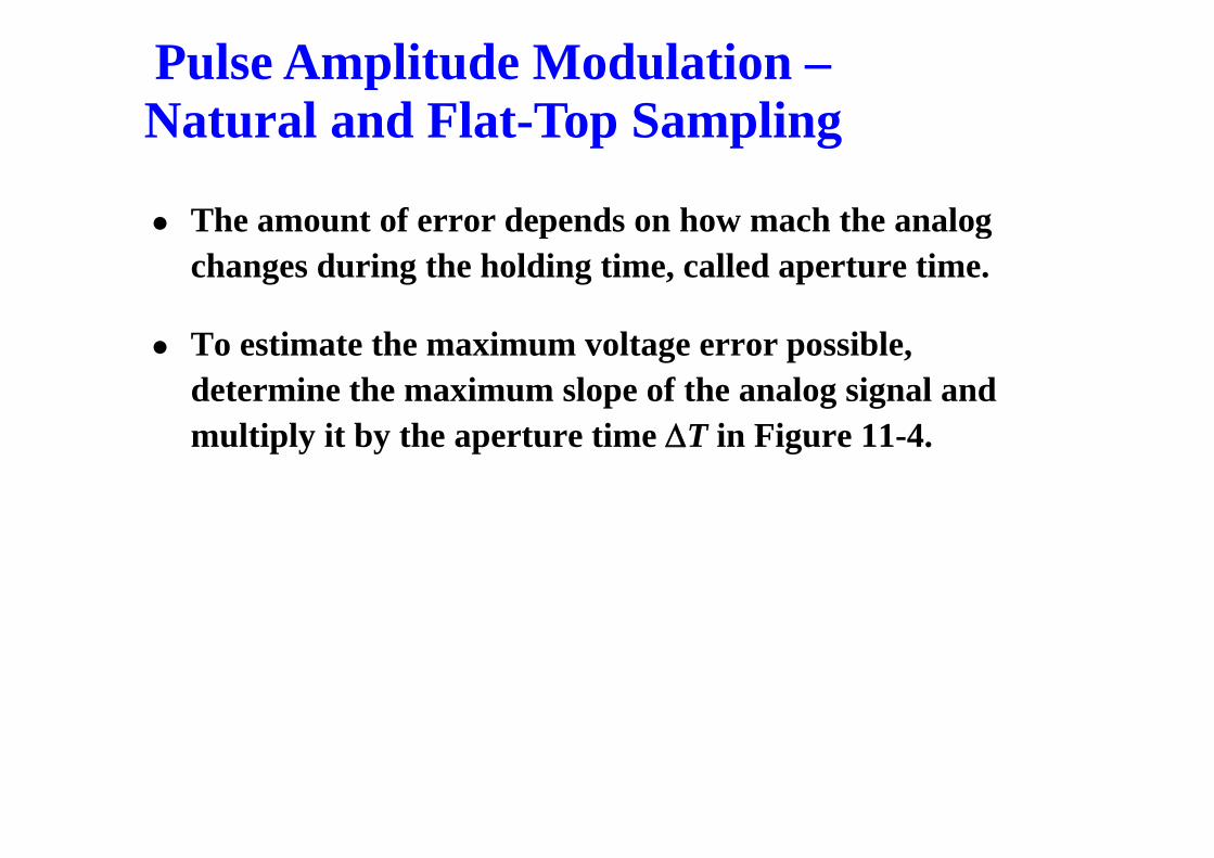
p gchanges during the holding time, called aperture time.

To estimate the maximum voltage error possible, determine the maximum slope of the analog signal and

lti l it b th t ti ΔT i Fi 11 4multiply it by the aperture time ΔT in Figure 11-4.


Figure 11-4. Sample-and-hold circuit and flat-top sampling.


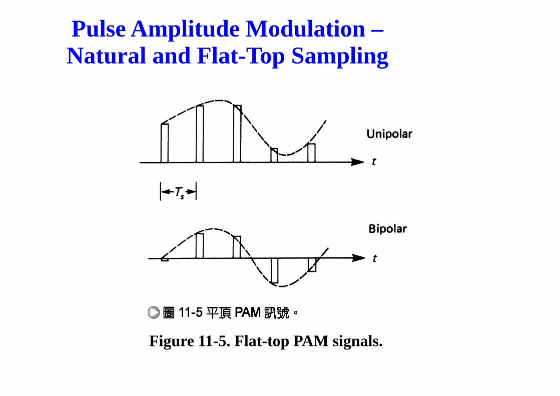
Figure 11-5. Flat-top PAM signals.

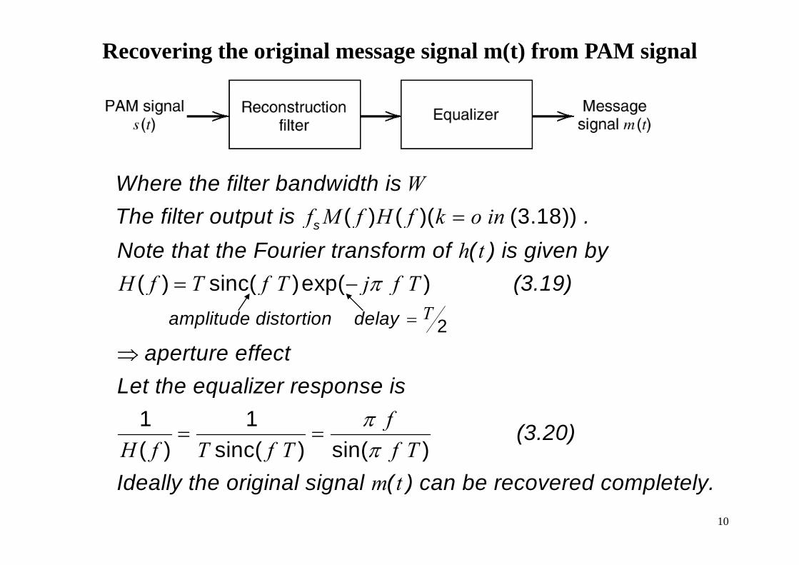
Recovering the original message signal m(t) from PAM signal

Wf M f H f k o in=

Where the filter bandwidth is The filter output is ( ) ( )( (3 18))f M f H f k o in

h tH f T f T j f Tπ

=

=

sThe filter output is . Note that the Fourier transform of ( ) is given by

(3 19)

( ) ( )( (3.18))

( ) sinc( )exp( )H f T f T j f Tπ= −

amplitude distort

(3.19)

( ) sinc( )exp( )T= ion delay

t ff t2

⇒ aperture effectLet the equalizer response is

1 1 fH f T f T f T

ππ

= = (3.20)

Id ll th i i l i l ( ) b d l t l

1 1( ) sinc( ) sin( )

m tIdeally the original signal ( ) can be recovered completely.10

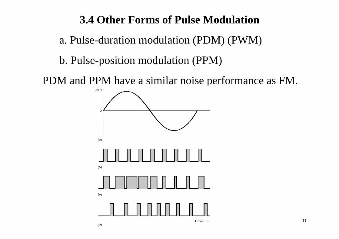
3.4 Other Forms of Pulse Modulation

P l d ti d l ti (PDM) (PWM)a. Pulse-duration modulation (PDM) (PWM)

b. Pulse-position modulation (PPM)p ( )

PDM and PPM have a similar noise performance as FM.

11

Pulse Width and Pulse Position Modulation

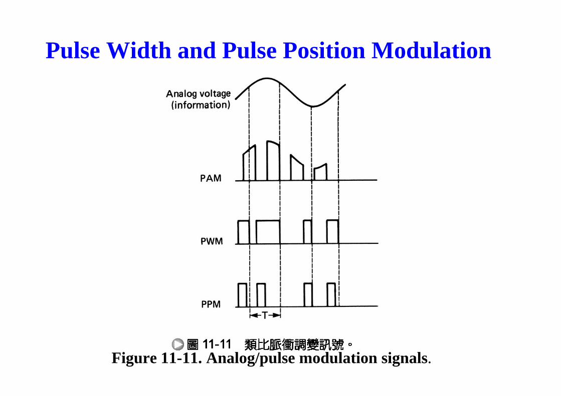
In pulse width modulation (PWM), the width of each pulse is made directly proportional to theeach pulse is made directly proportional to the amplitude of the information signal.

In pulse position modulation constant widthIn pulse position modulation, constant-width pulses are used, and the position or time of occurrence of each pulse from some reference ptime is made directly proportional to the amplitude of the information signal.

PWM and PPM are compared and contrasted to PAM in Figure 11-11.


Figure 11-11. Analog/pulse modulation signals.


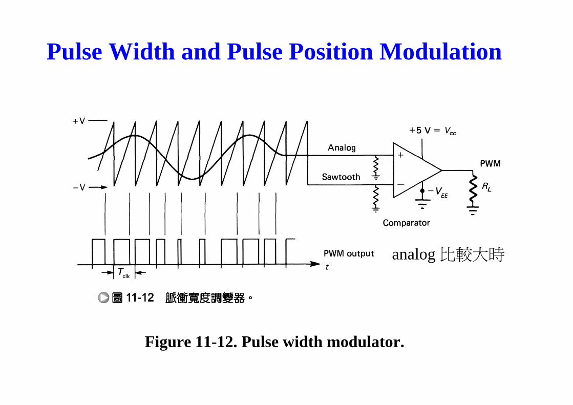
Fi 11 12 h PWM d l t Thi i itFigure 11-12 shows a PWM modulator. This circuit is simply a high-gain comparator that is switched on and off by the sawtooth waveform derived from ya very stable-frequency oscillator. Notice that the output will go to +Vcc the instant the analog signal exceeds the sawtooth voltagethe analog signal exceeds the sawtooth voltage.The output will go to -Vcc the instant the analog signal is less than the sawtooth voltage With thissignal is less than the sawtooth voltage. With this circuit the average value of both inputs should be nearly the same. Thi i il hi d ith l l i t tThis is easily achieved with equal value resistors to ground. Also the +V and –V values should not exceed Vcc.cc


l 比較大時analog 比較大時

Figure 11 12 Pulse width modulatorFigure 11-12. Pulse width modulator.


A 710-type IC comparator can be used for positive-only t t l th t l TTL tibl PWMoutput pulses that are also TTL compatible. PWM can

also be produced by modulation of various voltage-controllable multivibrators.

One example is the popular 555 timer IC. Other (pulse output) VCOs, like the 566 and that of the 565 phase-p ) , plocked loop IC, will produce PWM.

This points out the similarity of PWM to continuous p yanalog FM. Indeed, PWM has the advantages of FM---constant amplitude and good noise immunity---and also its disadvantage large bandwidthits disadvantage---large bandwidth.

Demodulation

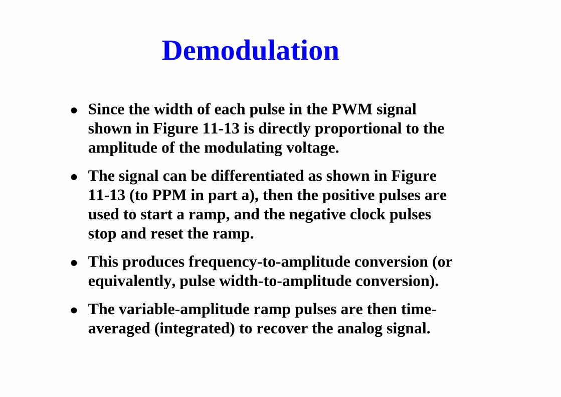
Since the width of each pulse in the PWM signalSince the width of each pulse in the PWM signal shown in Figure 11-13 is directly proportional to the amplitude of the modulating voltage.p g g

The signal can be differentiated as shown in Figure 11-13 (to PPM in part a), then the positive pulses are11 13 (to PPM in part a), then the positive pulses are used to start a ramp, and the negative clock pulses stop and reset the ramp.

This produces frequency-to-amplitude conversion (or equivalently, pulse width-to-amplitude conversion). q y, p p )

The variable-amplitude ramp pulses are then time-averaged (integrated) to recover the analog signal. g ( g ) g g


Figure 11-13. Pulse position modulator.

Demodulation

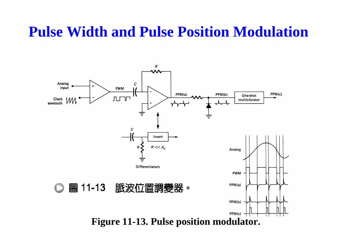
As illustrated in Figure 11-14, a narrow clock pulseAs illustrated in Figure 11 14, a narrow clock pulse sets an RS flip-flop output high, and the next PPM pulses resets the output to zero.

The resulting signal, PWM, has an average voltage proportional to the time difference between the PPM pulses and the reference clock pulses.PPM pulses and the reference clock pulses. Time-averaging (integration) of the output produces the analog variations.

PPM has the same disadvantage as continuous analog phase modulation: a coherent clock reference signal is necessary for demodulationreference signal is necessary for demodulation. The reference pulses can be transmitted along with the PPM signal.

Demodulation

This is achieved by full-wave rectifying the PPM pulses of Figure 11-13a, which has the effect of reversing the polarity of the negative (clock-rate) pulses.

Then an edge-triggered flipflop (J-K or D-type) can be used to accomplish the same function as the RS flip-flop of Figure 11-14, using the clock input.flop of Figure 11 14, using the clock input.

The penalty is: more pulses/second will require greater bandwidth and the pulse width limit the pulsebandwidth, and the pulse width limit the pulse deviations for a given pulse period.

Demodulation

Figure 11-14. PPM demodulator.

Pulse Code Modulation (PCM)Pulse Code Modulation (PCM)

Pulse code modulation (PCM) is produced by analog-( ) p y gto-digital conversion process.

As in the case of other pulse modulation techniques, theAs in the case of other pulse modulation techniques, the rate at which samples are taken and encoded must conform to the Nyquist sampling rate.

The sampling rate must be greater than, twice the highest frequency in the analog signal, g q y g g ,

fs > 2fA(max)

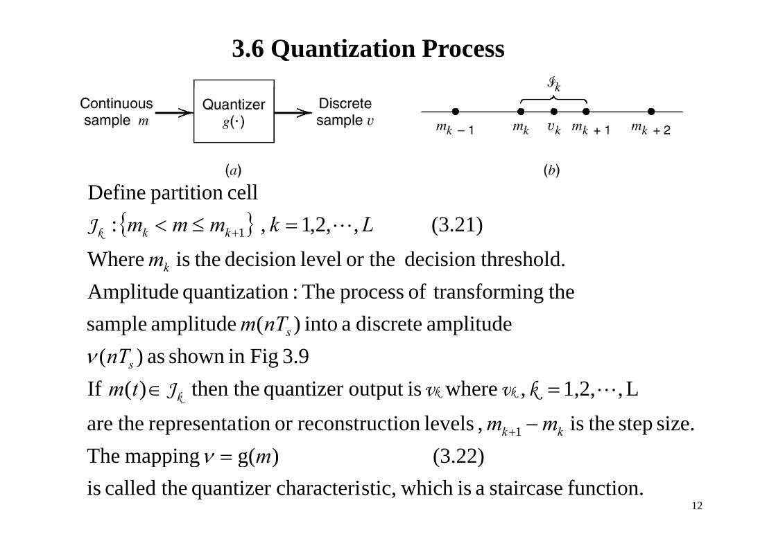
3.6 Quantization Process

{ }cell partition Define

{ }. thresholddecision or the level decision theis Where

(3.21) ,,2,1 , : 1

mLkmmm

k

kk =≤< + LJk

amplitude discretea into )( amplitude sample theing transformof process The:onquantizati Amplitude

nTm s

L,1,2,,whereisoutput quantizer the then)( If3.9 Figin shown as )(

tmnTs

=∈ν

LkννJ kkk

(3 22))g(mappingThesize. step theis , levels tionreconstrucor tionrepresenta theare

,, ,,pq)(

1

mmm kk

=−+

ν

kk

function. staircasea is whichstic,characteriquantizer thecalled is(3.22) )g( mappingThe mν

12

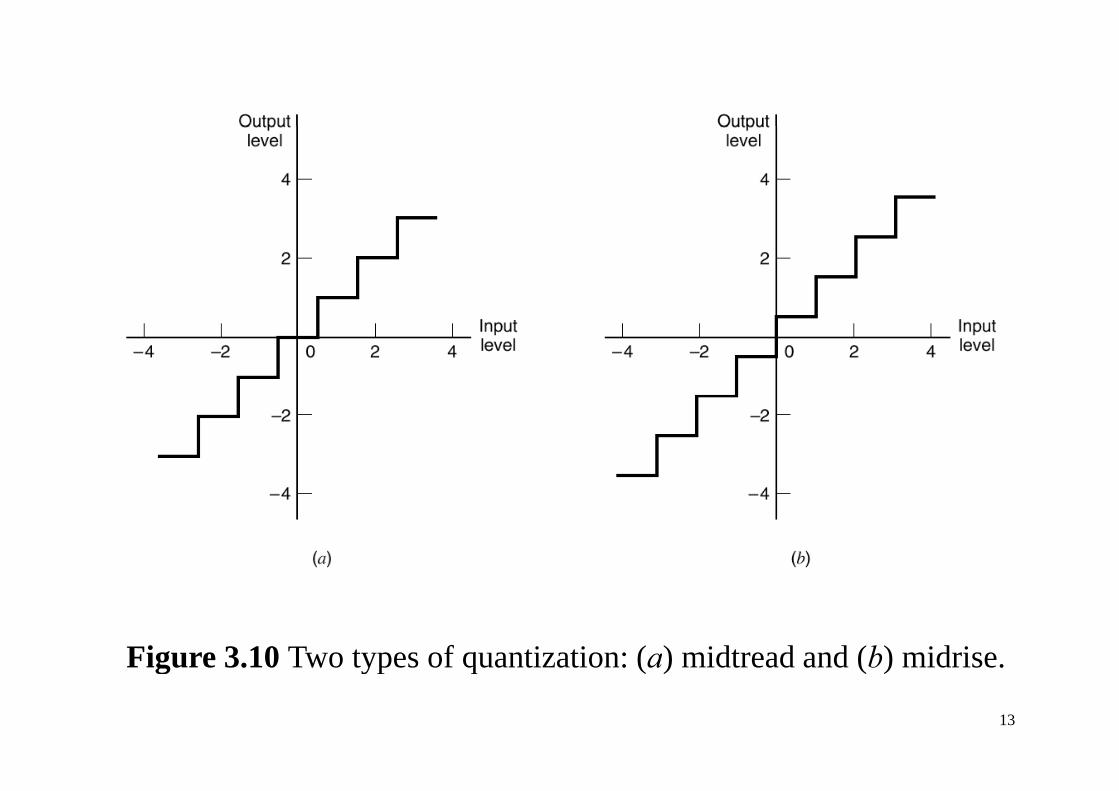
Figure 3.10 Two types of quantization: (a) midtread and (b) midrise.Figure 3.10 Two types of quantization: (a) midtread and (b) midrise.

13

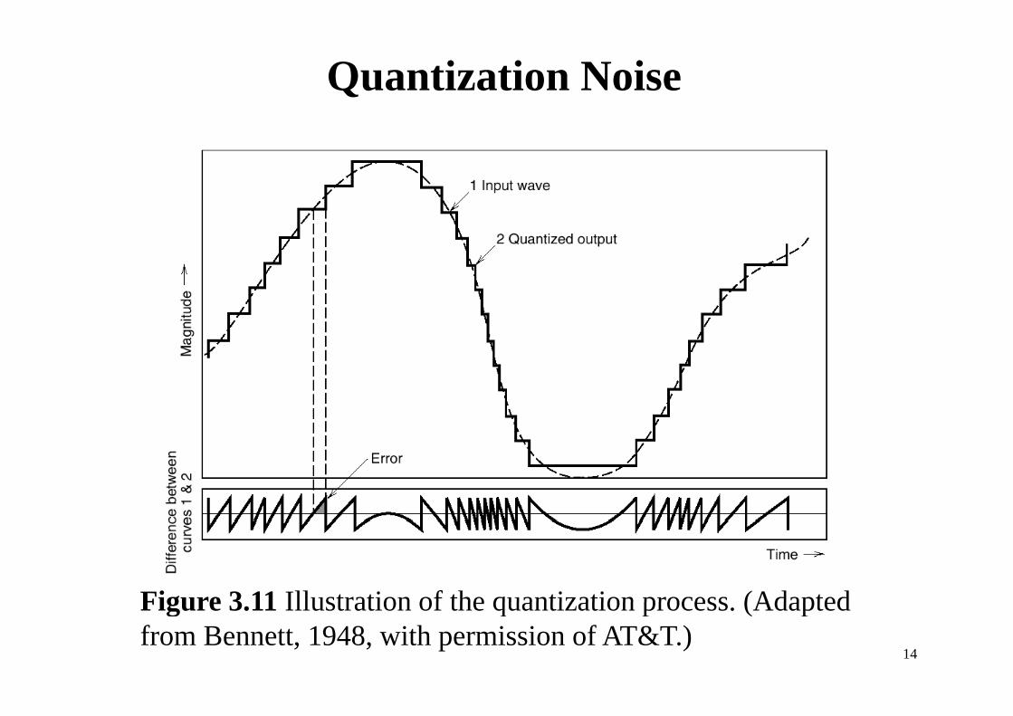
Quantization Noise

Figure 3 11 Illustration of the quantization process (AdaptedFigure 3.11 Illustration of the quantization process. (Adapted from Bennett, 1948, with permission of AT&T.)

14

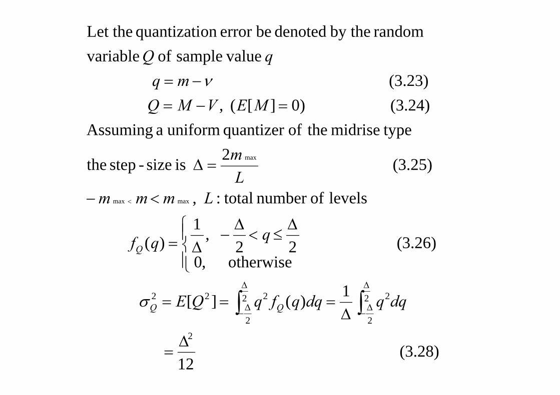
valuesampleof variablerandomby the denotedbeerror onquantizati Let the

qQ

(3 24))0][((3.23)

p

=−=−=

MEVMQmq

qQν

2 typemidrise theofquantizer uniforma Assuming

(3.24) )0][( , ==

m

MEVMQ

levelsofnumbertotal:

(3.25) 2 is size-step the max

<

=Δ

LmmmL

m

(3 26)22,1

)(

levels ofnumber total: , max max

⎪⎨⎧ Δ

≤<Δ

−Δ=

<− <

qqf

Lmmm

1

(3.26) otherwise

22 ,0

)( ⎪⎩⎨Δ=

ΔΔ

qqfQ

1)(][ 2

2

22

2

222

Δ=== ∫∫

Δ

Δ−

Δ

Δ−

dqqdqqfqQE QQσ

(3.28) 12

2Δ

=

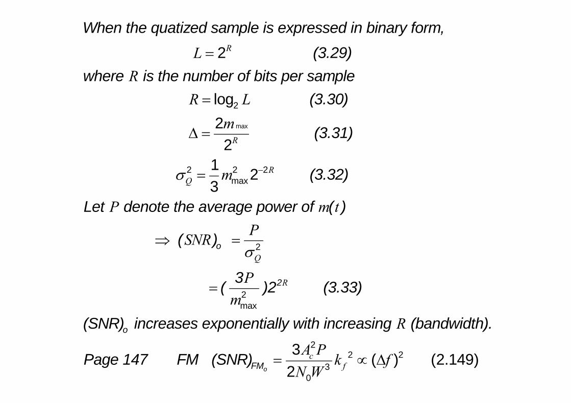
When the quatized sample is expressed in binary form, (3.29)2RL =where is the number of bits per sample (3.302log

RR L= )

(3.31)max22R

mΔ =

(3.32)

L t d t th f ( )

2 2 2max

1 23

RQ mσ −=

o

Let denote the average power of ( )

( ) 2

P m tPSNR⇒ =o( )

2Qσ

23 ( )2 (3.33)2RP

=

o

( ) ( )

(SNR) increases exponentially with increasing (bandwidth).

2maxm

R

oFMPage 147 FM (SNR)2

2 23

0

3 ( ) (2.149)2

cf

A P k fN W

= ∝ Δ

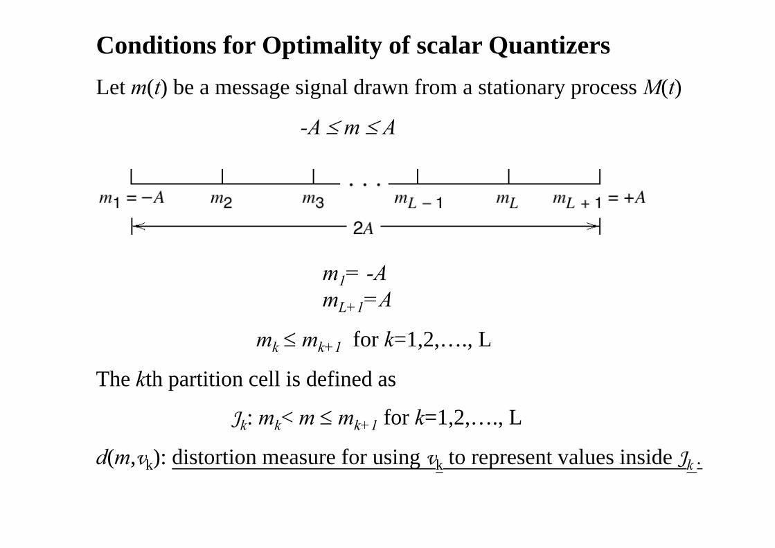
Conditions for Optimality of scalar QuantizersLet m(t) be a message signal drawn from a stationary process M(t)Let m(t) be a message signal drawn from a stationary process M(t)

-A ≤ m ≤ A

m = Am1= -AmL+1=A

≤ for k 1 2 Lmk ≤ mk+1 for k=1,2,…., L

The kth partition cell is defined as

Jk: mk< m ≤ mk+1 for k=1,2,…., L

d(m vk): distortion measure for using vk to represent values inside Jkd(m,vk): distortion measure for using vk to represent values inside Jk .

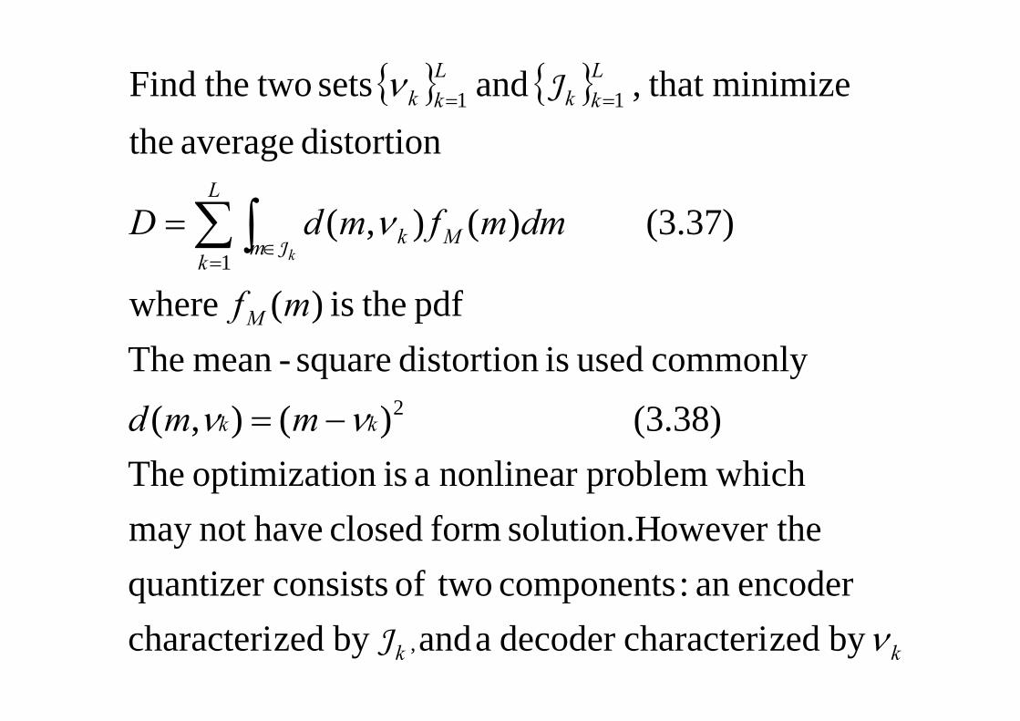
{ } { }Lkk

Lkkν minimize that , and sets two theFind 11 J ==

L

distortion average the

Mk

m k dmmfmdDk

ν (3.37) )(),(1

J= ∑∫

=∈

M mfcommonlyusedisdistortionsquaremeanThe

pdf theis )( where

kk mmd νν (3.38) )( ),(commonlyused isdistortionsquare-meanThe

2−=

o e er thesol tion Hformclosedha enotma whichproblemnonlinear a is onoptimizati The

encoder an: components twoof consistsquantizer owever thesolution.Hformclosedhavenot may

kk νby zedcharacteridecoder a andby zedcharacteri ,J

{ } { } DminimizesthatsetthefindsettheGiven

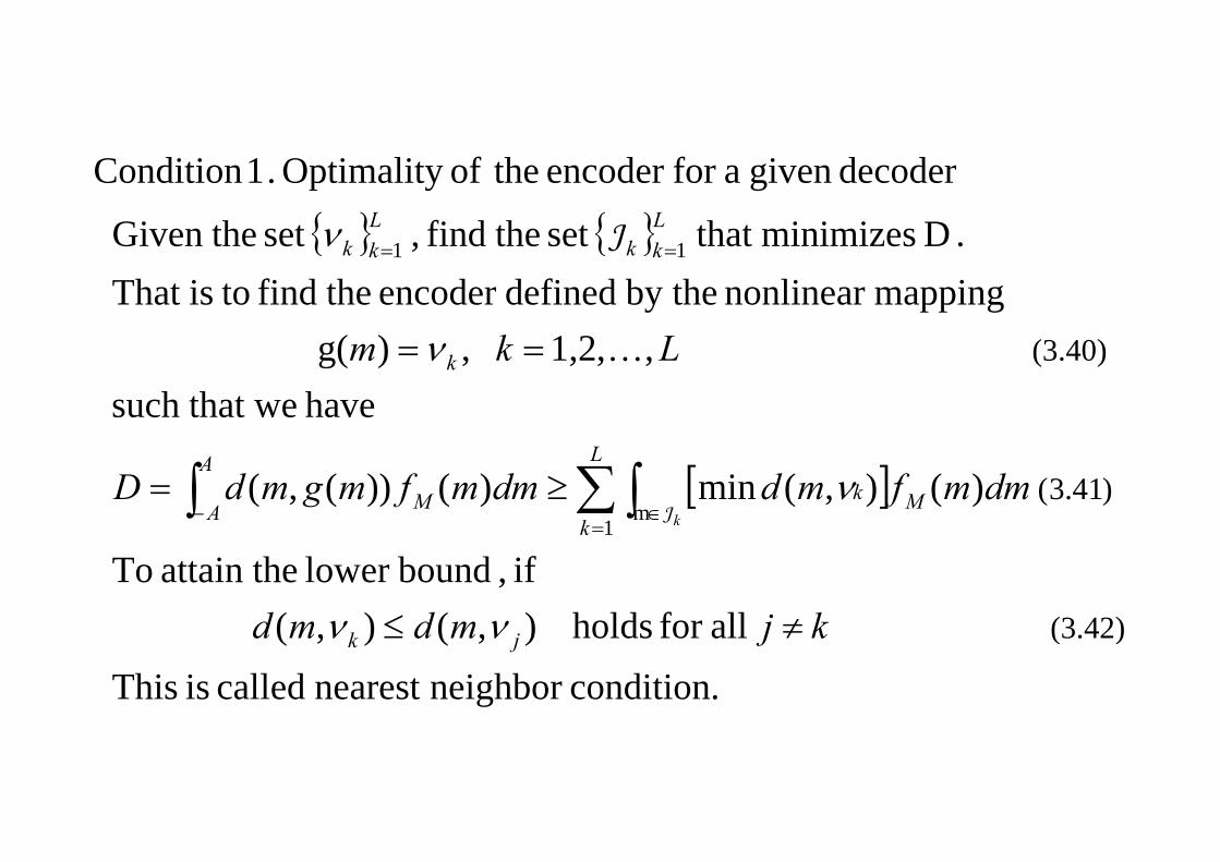
decodergivena for encoder theofOptimality . 1ConditionLLν J{ } { }

mappingnonlinear by the definedencoder thefind toisThat .Dminimizes that set thefind,set theGiven 11 kkkk ==ν J

have that wesuch ,,1,2 ,)g( (3.40)Lkm k ==ν K

[ ] )(),(min)())(,( )41.3(1

mdmmfmddmmfmgmdD M

L

k

kA

A Mk

≥= ∑∫∫=

∈−ν

J

allforholds)()( if , boundlower theattain To

(3 42)

1

kjmdmd

k

≠≤

=

νν

condition.neighbor nearest called is This allfor holds ),(),( (3.42)kjmdmd jk ≠≤ νν

{ } { }L L D

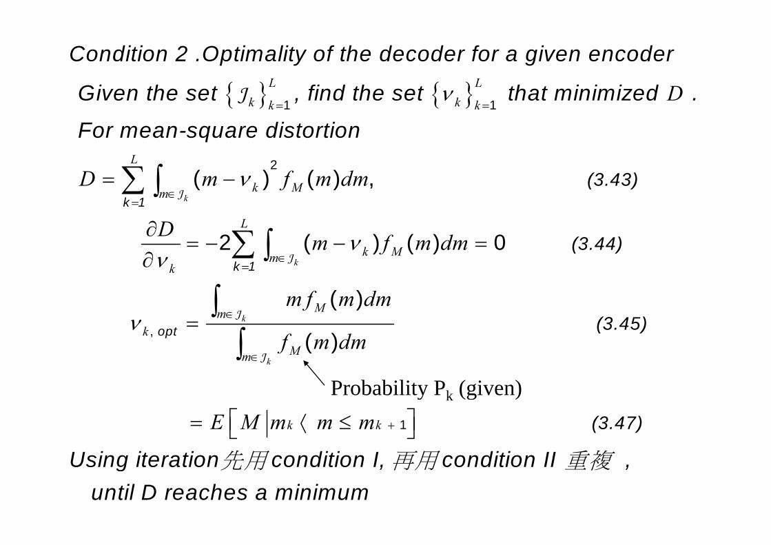
Condition 2 .Optimality of the decoder for a given encoder

Gi th t fi d th t th t i i i d{ } { }k kk kDν

= = Given the set , find the set that minimized .

For mean-square distortion1 1

J

k

L

k MmD m f m dmν

∈=

= −∑ ∫k 1

(3.43) 2

( ) ( ) ,J

k

L

k Mmk

D m f m dmνν ∈

=

∂= − − =

∂ ∑ ∫k 1

(3.44) 2 ( ) ( ) 0J

k

k

Mmk

m f m dm

f dν ∈=

∫∫

opt (3.45)

,

( )

( )J

k

kMm

f m dm∈∫

opt, ( )J

Probability Pk (given)k kE M m m m +⎡ ⎤= ⟨ ≤⎣ ⎦ (3.47)

Usi

1

ng iteration condition I condition II先用再用重複

y k (g )

Using iteration condition I, condition II , until D reaches a minimum

先用再用重複

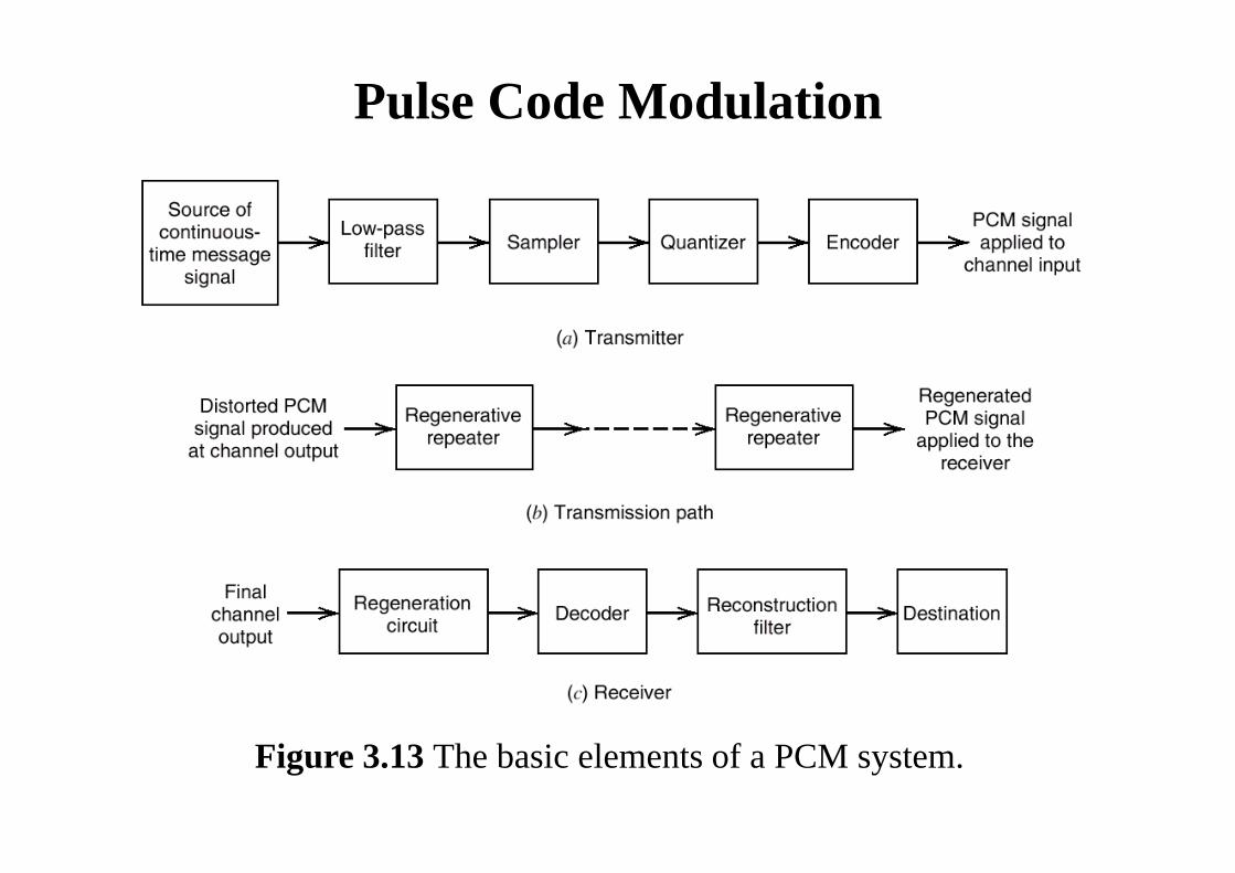
Pulse Code Modulation

Figure 3.13 The basic elements of a PCM system.

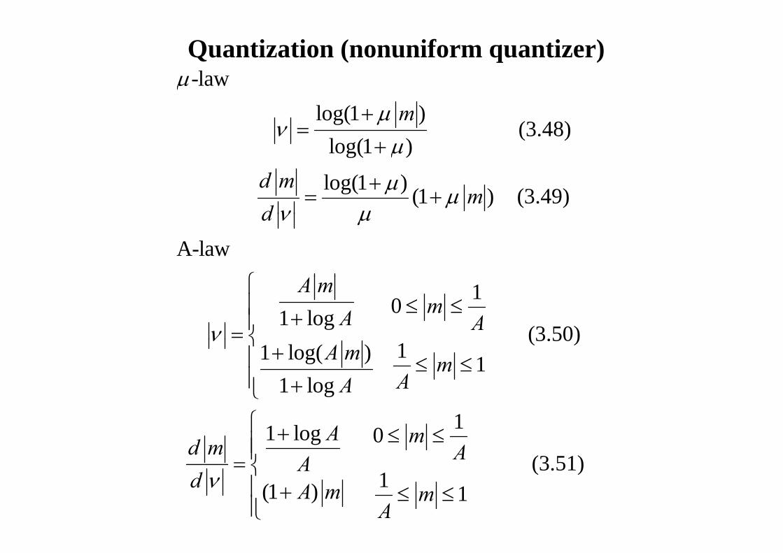
-lawμQuantization (nonuniform quantizer)

log(1 ) (3.48)

log(1 )m

μμ

νμ

+=

+log(1 )

log(1 ) (1 ) (3.49)d m

md

μ

μ μν μ

+

+= +

A-lawd ν μ

⎧ 101 log(3.50)

A mmA Aν

⎧≤ ≤⎪ +⎪= ⎨ (3.50)

11 log( ) 11 log

A m mAA

ν ⎨+⎪ ≤ ≤

⎪ +⎩

1 log 0Ad mA

+=

1

(3 51)m

A⎧ ≤ ≤⎪⎪⎨

(1 )A

d A mν=

+ (3.51)

1 1mA

⎨⎪ ≤ ≤⎪⎩

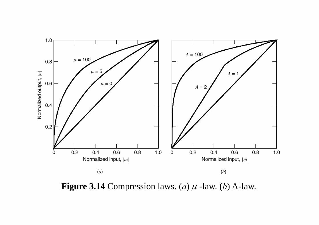
Figure 3.14 Compression laws. (a) μ -law. (b) A-law.Figure 3.14 Compression laws. (a) μ law. (b) A law.

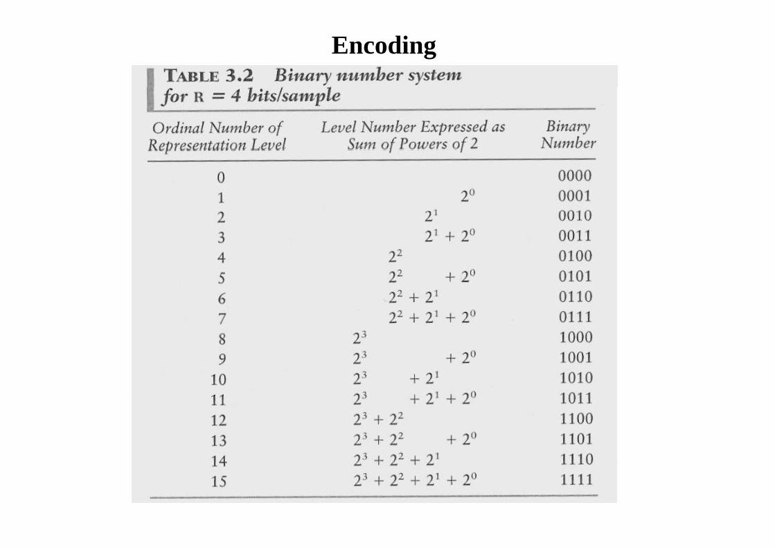
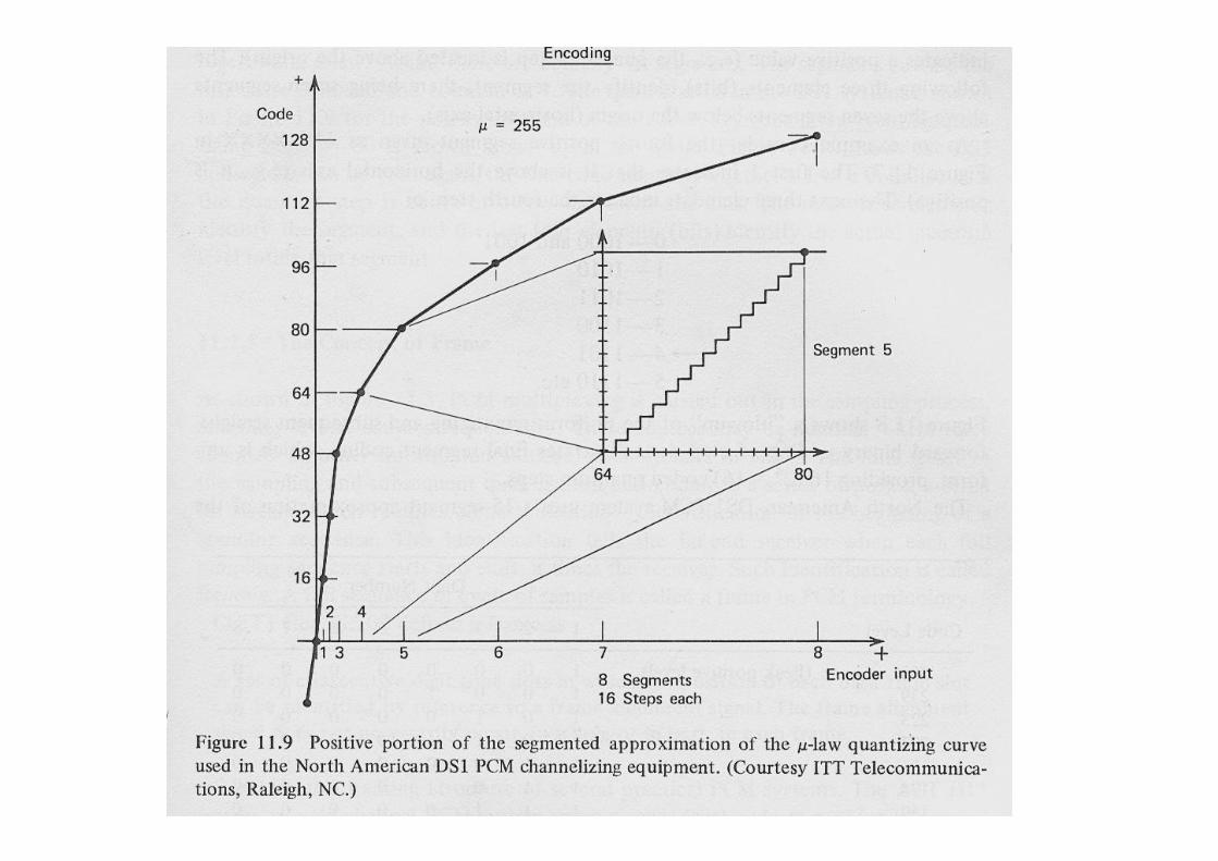
Encoding

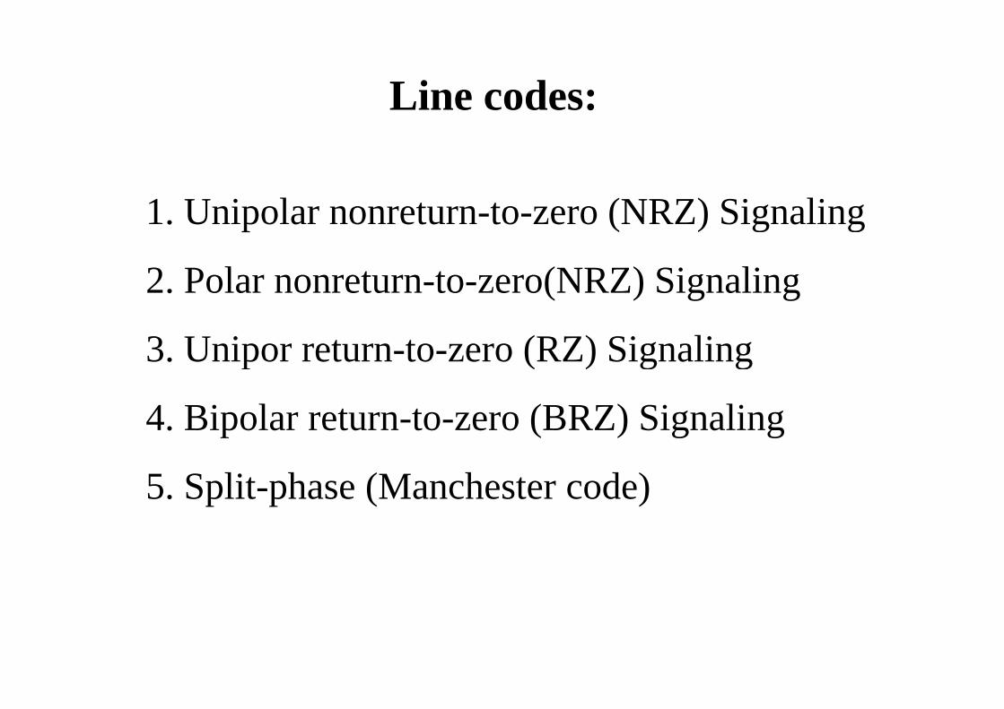
Line codes:

1. Unipolar nonreturn-to-zero (NRZ) Signaling

2 P l t t (NRZ) Si li2. Polar nonreturn-to-zero(NRZ) Signaling

3 Unipor return-to-zero (RZ) Signaling3. Unipor return to zero (RZ) Signaling

4. Bipolar return-to-zero (BRZ) Signaling p ( ) g g

5. Split-phase (Manchester code)

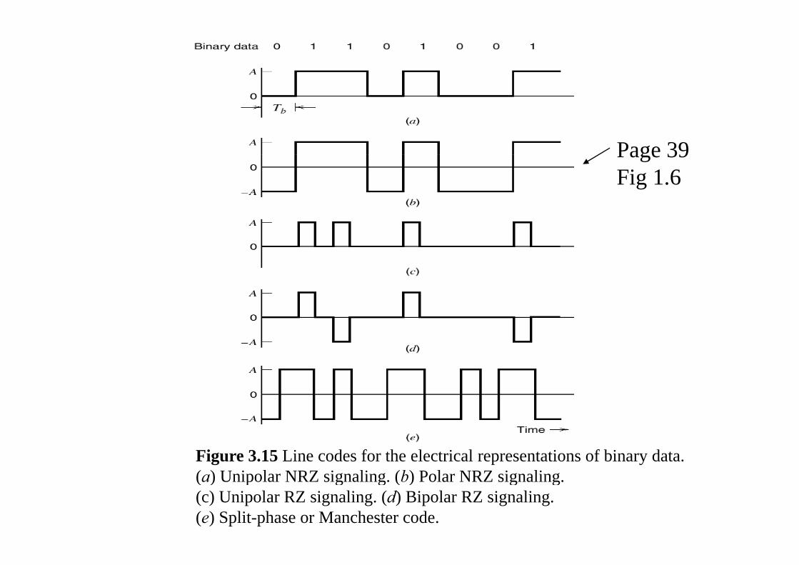
Page 39Fig 1.6

Figure 3.15 Line codes for the electrical representations of binary data. (a) Unipolar NRZ signaling (b) Polar NRZ signaling(a) Unipolar NRZ signaling. (b) Polar NRZ signaling.(c) Unipolar RZ signaling. (d) Bipolar RZ signaling. (e) Split-phase or Manchester code.

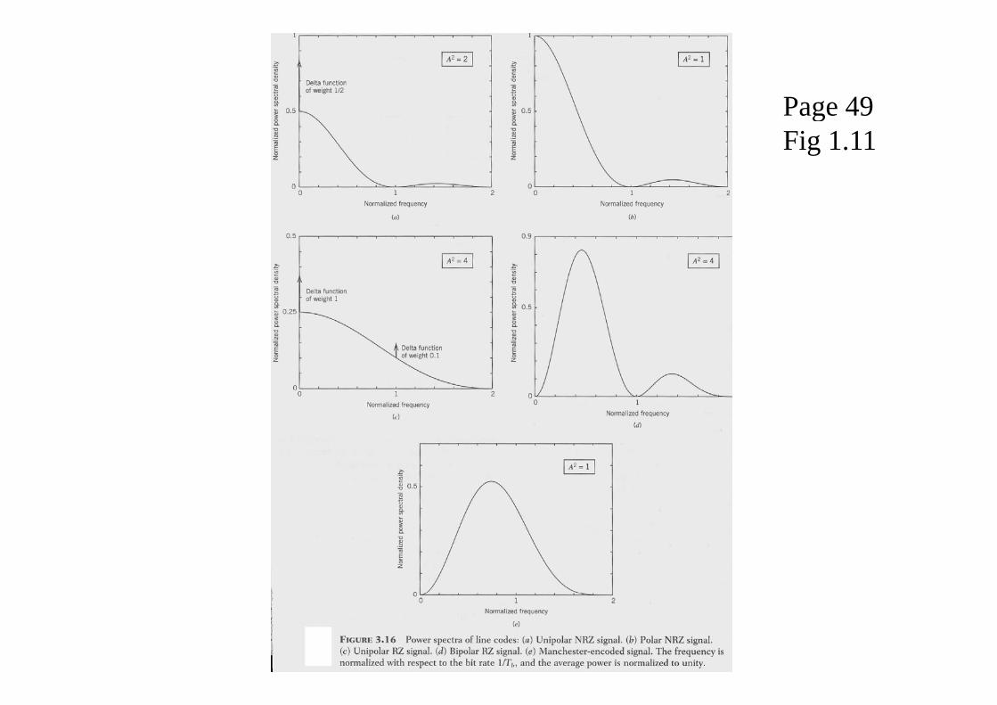
Page 49Fig 1.11

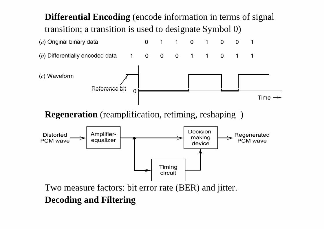
Differential Encoding (encode information in terms of signal transition; a transition is used to designate Symbol 0)

Regeneration (reamplification retiming reshaping )Regeneration (reamplification, retiming, reshaping )

Two measure factors: bit error rate (BER) and jitter. ( ) jDecoding and Filtering

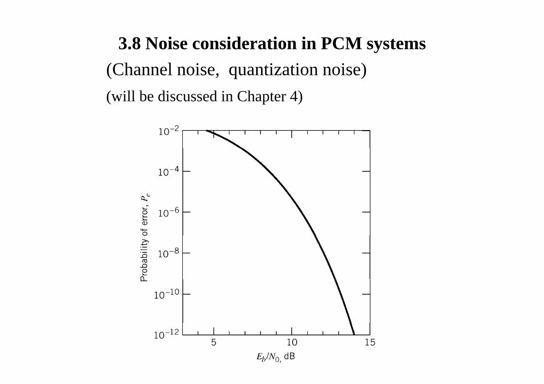
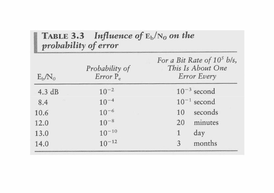
3.8 Noise consideration in PCM systems(Channel noise, quantization noise)(will be discussed in Chapter 4)

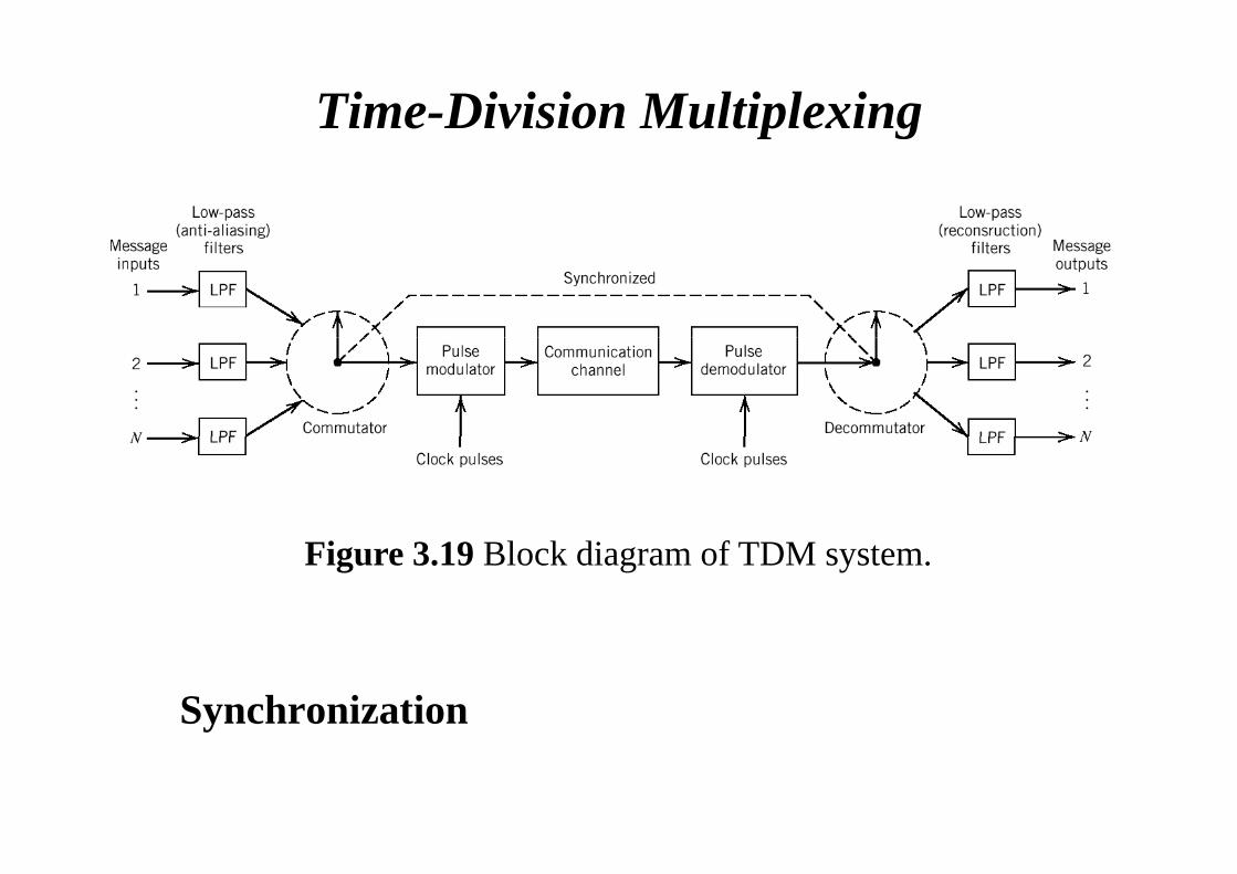
Time-Division Multiplexing

Figure 3.19 Block diagram of TDM system.

Synchronization

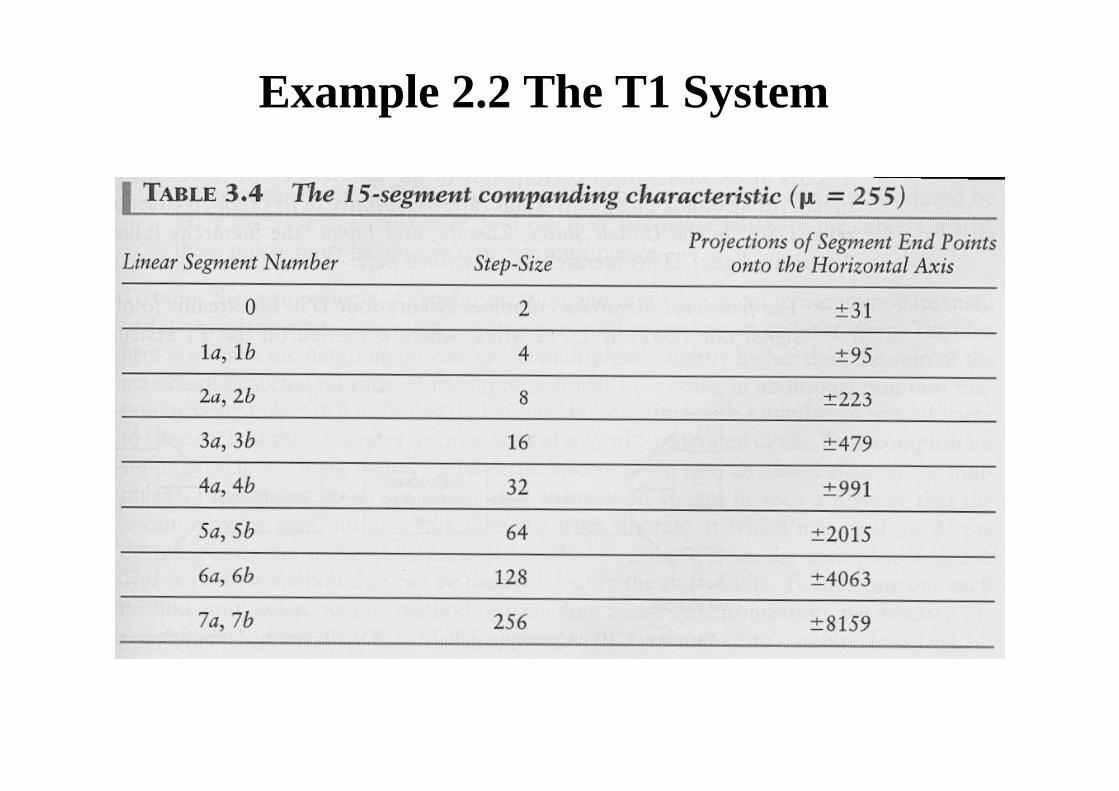
Example 2.2 The T1 System

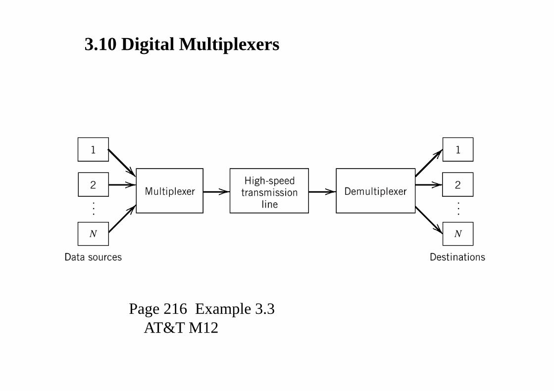
3.10 Digital Multiplexers

Page 216 Example 3.3AT&T M12AT&T M12

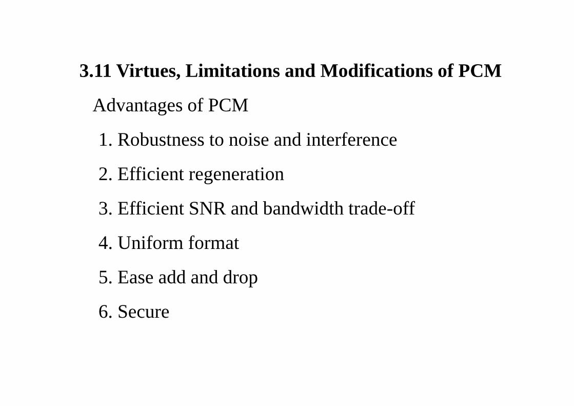
3 11 Vi Li i i d M difi i f PCM3.11 Virtues, Limitations and Modifications of PCM

Advantages of PCMAdvantages of PCM

1. Robustness to noise and interference

2. Efficient regeneration

3 Effi i SNR d b d id h d ff3. Efficient SNR and bandwidth trade-off

4. Uniform format . U o o

5. Ease add and drop

6. Secure

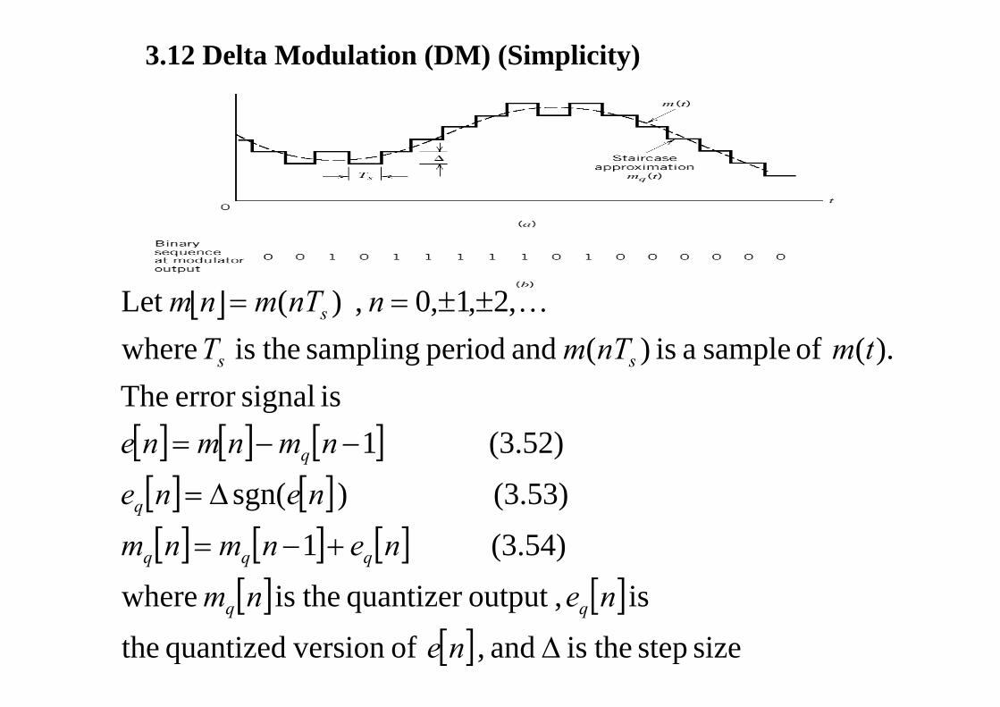
3.12 Delta Modulation (DM) (Simplicity)

[ ])(ofsampleais)(andperiodsamplingtheiswhere

,2,1,0 , )(Let ±±==tmnTmT

nnTmnm s K

[ ] [ ] [ ] (3 52)1 is signalerror The

).(ofsampleais)( andperiodsampling theiswhere tmnTmT ss

[ ] [ ] [ ][ ] [ ] (3.53) ) sgn(

(3.52) 1

Δ=

−−=

nene

nmnmne

q

q

[ ] [ ] [ ][ ] [ ]isoutputquantizertheiswhere

(3.54) 1 +−=

nenm

nenmnm qqq

q

[ ] [ ][ ] size step theis and , of version quantized the

is,output quantizer theis where

Δne

nenm qq

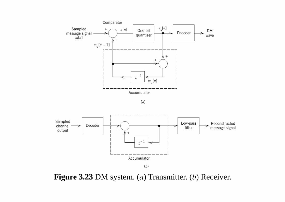
Figure 3.23 DM system. (a) Transmitter. (b) Receiver.

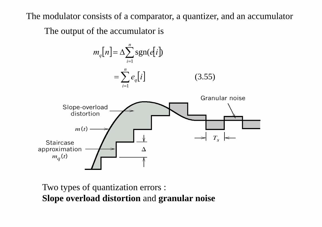
The modulator consists of a comparator, a quantizer, and an accumulatorThe output of the accumulator is

[ ] [ ])sgn(1∑=

Δ=n

iq ienm

[ ] (3.55) 1

1

∑=

=n

iq

i

ie

Two types of quantization errors :yp qSlope overload distortion and granular noise

[ ]byerroronquantizatitheDenote nqSlope Overload Distortion and Granular Noise

[ ][ ] [ ] [ ] (3.56)

,by error onquantizati theDenotenqnmnm

nq

q −=

[ ] [ ] [ ] [ ] (3 57)11 have we, (3.52) Recall

nqnmnmne =[ ] [ ] [ ] [ ][ ] first a isinput quantizer the,1for Except

(3.57) 11 nq

nqnmnmne−

−−−−=

requirewedistortionoverload-slopeavoidTosignalinput theof difference backward ( differentiator )

(3.58))(max(slope)

requirewe,distortionoverloadslope avoidTotdm

≥Δ

sizestepwhenoccurs noisegranular hand,other theOn

(3.58) max (slope)dtTs

≥

.)( of slope local the torelative large toois pg,

tmΔ

Delta-Sigma modulation (sigma-delta modulation)The modulation which has an integrator can relieve the draw back of delta modulation (differentiator)

Σ−Δ

Beneficial effects of using integrator:1. Pre-emphasize the low-frequency content2. Increase correlation between adjacent samples (reduce the variance of the error signal at the quantizer input )

3. Simplify receiver design

Because the transmitter has an integrator , the receiverBecause the transmitter has an integrator , the receiver consists simply of a low-pass filter. (The accumulator in the conventional DM receiver is cancelled by(The accumulator in the conventional DM receiver is cancelled by the differentiator )

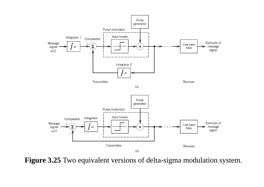
Figure 3.25 Two equivalent versions of delta-sigma modulation system.

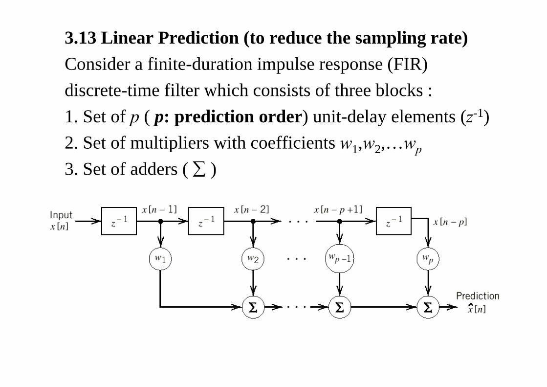
3.13 Linear Prediction (to reduce the sampling rate)Consider a finite duration impulse response (FIR)Consider a finite-duration impulse response (FIR) discrete-time filter which consists of three blocks :1. Set of p ( p: prediction order) unit-delay elements (z-1) 2. Set of multipliers with coefficients w1,w2,…wpp 1, 2, p

3. Set of adders ( ∑ )

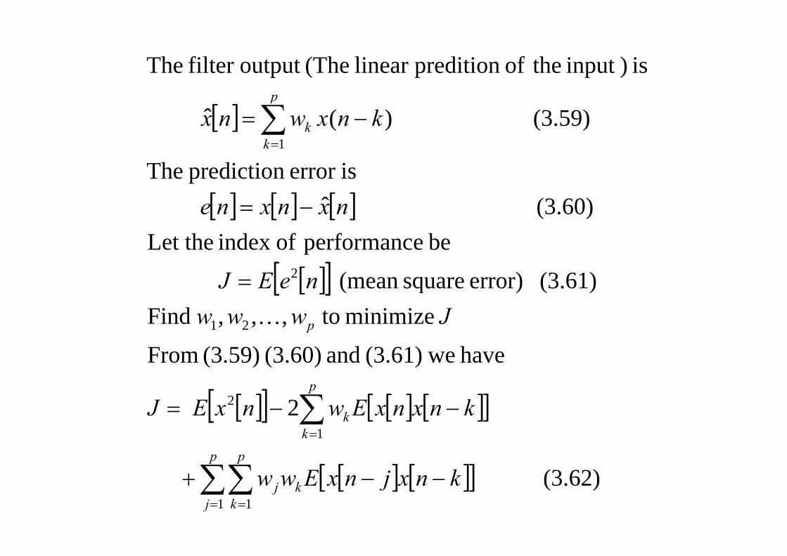
is )input theof preditionlinear (Theoutput filter The

[ ] (3.59) )(ˆ 1

∑=

−=p

kk knxwnx

[ ] [ ] [ ] (3.60) ˆ iserror prediction The

−= nxnxne[ ] [ ] [ ]

[ ][ ] (3 61)error)square(mean be eperformanc ofindex Let the

( )

2 neEJ [ ][ ] minimize to,,, Find

(3.61) error)square(mean

21

=

p JwwwneEJ

K

[ ][ ] [ ] [ ][ ]2

have we(3.61) and (3.60) (3.59) From

2 ∑p

kEEJ [ ][ ] [ ] [ ][ ]

[ ] [ ][ ]

21

2

∑∑

∑=

−−=

p pk

k knxnxEwnx EJ

[ ] [ ][ ] (3.62) 1 1∑∑= =

−−+j k

kj knxjnxEww

[ ][ ] [ ][ ])(0)]][[( mean zero withprocess stationary is )( Assume

222 nxEnxEnxEtX

−=

=

σ [ ][ ] [ ][ ][ ][ ]

)( 2 nxE

nxEnxEX

=

−=σ

[ ] [ ] [ ][ ])( ationautocorrelThe

knxnxEkRkTR XsX −===τ

[ ] [ ]

as simplify may We

2

Jp pp

∑∑∑ [ ] [ ] (3.63) 2 1 11

2

J

jkRwwkRwJ

p

j kXkj

kXkX

∂

−+−= ∑∑∑= ==

σ

[ ] [ ] 022 1

jkRwkRwJ p

jXjX

k

=−+−=∂∂ ∑

=

[ ] [ ] [ ] (3.64) 21 , 1

,p,,kkRkRjkRwp

jXXXj K=−==−∑

=

equations Hopf-Wiener called are (3.64)1j

[ ]

10

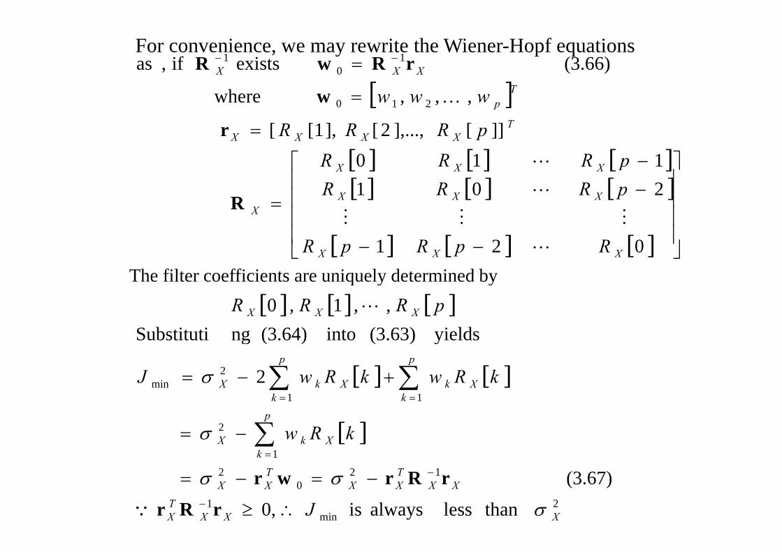
1 (3.66) exists if , asT

XXX = −− rRwRFor convenience, we may rewrite the Wiener-Hopf equations

[ ]

[ ] [ ] [ ]

210

]][],...,2[ ],1[[

,,, where T

XXXX

Tp

pRRR

www

⎤⎡

=

=

r

w K

[ ] [ ] [ ][ ] [ ] [ ]201

110

XXX

XXX

X

pRRRpRRR

⎥⎥⎥⎤

⎢⎢⎢⎡

−−

=RMMM

L

L

[ ] [ ] [ ]021 XXX

X

RpRpR ⎥⎥

⎦⎢⎢

⎣ −− L

MMM

The filter coefficients are uniquely determined by[ ] [ ] [ ]

yields(3.63)into(3.64)ngSubstituti,, 1, 0 XXX pRRR L

The filter coefficients are uniquely determined by

[ ] [ ]11

2min 2

yields(3.63)into(3.64)ngSubstitutip

kXk

p

kXkX kRwkRwJ σ +−=

==∑∑

[ ]1

2 p

kXkX kRwσ −=

=∑

2min

1

12

02

thanless always is 0,

(3.67)

XXXTX

XXTXX

TXX

J σ

σσ

∴≥

−=−=−

−

rRr

rRrwr

Q

f llthid tiidi tTh

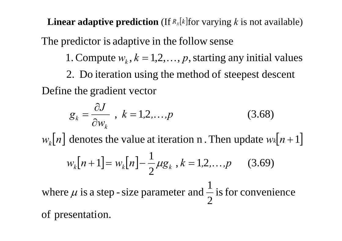
[ ] kRXLinear adaptive prediction (If for varying k is not available)

valuesinitialany starting ,,,2,1 , Compute 1. sensefollow theinadaptiveispredictor The

pkwk K=

ectorgradient vtheDefinedescentsteepest of method theusing iteration Do2.

(3.68) 21 ,

ectorgradient v theDefine

,p,,kJgk K=∂∂

=

[ ] [ ]1 update Then . n iterationat value thedenotes nwnww

kk

k

+∂

[ ] [ ] (3.69) 21 ,211 μ ,p,,kgnwnw kkk K=−=+

econveniencfor is 21 andparameter size-stepa is where μ

on.presentati of2

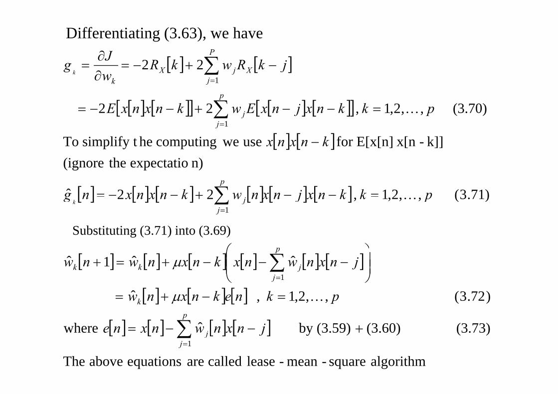
[ ] [ ]22 +∂ ∑ jkRkRJ P

Differentiating (3.63), we have

[ ] [ ]

[ ] [ ][ ] [ ] [ ][ ] (3 70)2122

22 1

+

−+−=∂

=

∑

∑=

pkknxjnxEwknxnxE

jkRwkRw

g

p

jXjX

kk

[ ] [ ][ ] [ ] [ ][ ]

[ ] [ ] k]]-x[nfor E[x[n] use wecomputing hesimplify t To

(3.70) ,,2,1,22 1

−

=−−+−−= ∑=

knxnx

pkknxjnxEwknxnxEj

j K

[ ] [ ] [ ] [ ] [ ] [ ] )713(2122ˆ

n)expectatio the(ignore

=−−+−−= ∑ pkknxjnxnwknxnxngp

[ ] [ ] [ ] [ ] [ ] [ ] )71.3( ,,2,1,221

+ ∑=

pkknxjnxnwknxnxngj

jkK

Substituting (3.71) into (3.69)

[ ] [ ] [ ] [ ] [ ] [ ]ˆˆ1ˆ1

⎟⎟⎠

⎞⎜⎜⎝

⎛−−−+=+ ∑

=

jnxnwnxknxnwnwp

jjkk μ

[ ] [ ] [ ]

[ ] [ ] [ ] [ ] (3 73)(3 60)(3 59)byˆwhere

)72.3( ,,2,1 , ˆ

+−−=

=−+=

∑ jnxnwnxne

pkneknxnwp

j

k Kμ

[ ] [ ] [ ] [ ]

algorithm square-mean-lease called are equations above The

(3.73) (3.60)(3.59)by where 1

+∑=

jnxnwnxnej

j

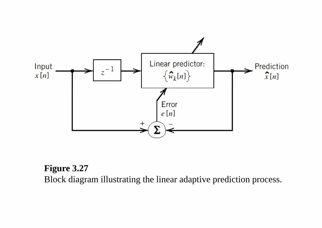
Fi 3 27Figure 3.27Block diagram illustrating the linear adaptive prediction process.

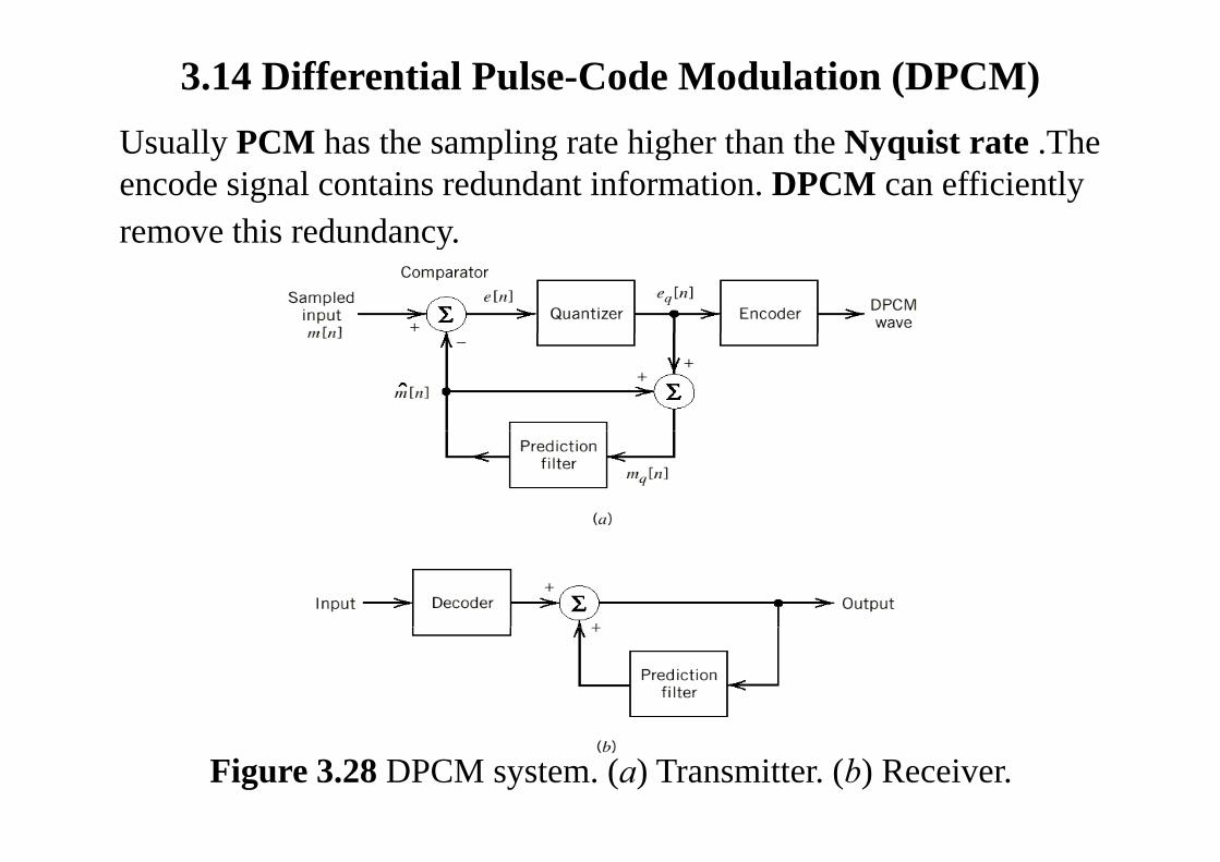
3.14 Differential Pulse-Code Modulation (DPCM)Us all PCM has the sampling rate higher than the Nyquist rate TheUsually PCM has the sampling rate higher than the Nyquist rate .The encode signal contains redundant information. DPCM can efficiently remove this redundancyremove this redundancy.

Figure 3.28 DPCM system. (a) Transmitter. (b) Receiver.

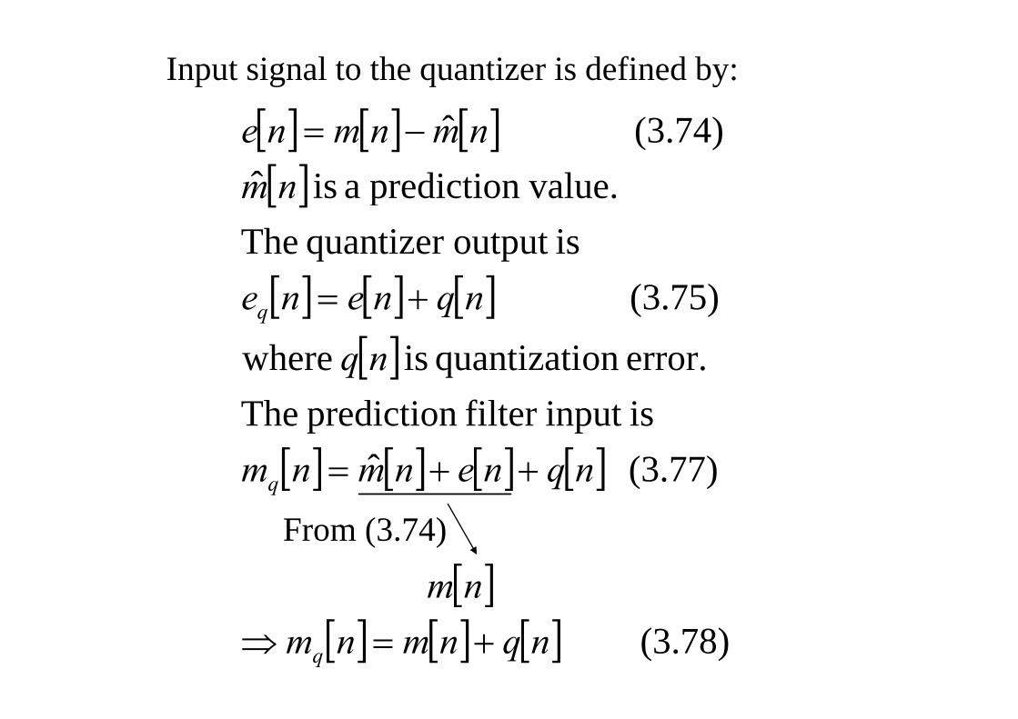
Input signal to the quantizer is defined by:

[ ] [ ] [ ][ ] [ ] [ ][ ] value.predictionaisˆ

(3.74) ˆnm

nmnmne −=[ ]

[ ] [ ] [ ] isoutput quantizer The

value.predictiona isnm

[ ] [ ] [ ][ ] erroronquantizatiiswhere

(3.75) nq

nqneneq +=

[ ]isinput filter prediction Theerror.onquantizatiiswhere nq

[ ] [ ] [ ] [ ] (3.77) ˆ nqnenmnmq ++=

F (3 74)

[ ]

nmFrom (3.74)

[ ][ ] [ ] [ ] (3.78) nqnmnmq +=⇒

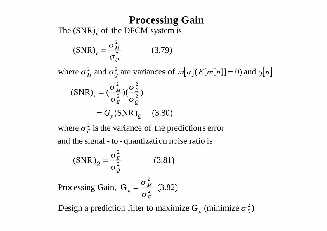
is system DPCM theof (SNR) The o

Processing Gain

(3.79) (SNR) 2

2

oQ

M

σσ

=

[ ] [ ]

))(((SNR)

and 0)]][[( of variancesare and where22

22

EM

QM nqnmEnm

σσ

σσ =

(3.80))SNR(

))(((SNR)

22o

Qp

Q

E

E

M

Gσσ

σσ

=

=

isrationoiseonquantizati-to-signaltheanderror sprediction theof variance theis where

(3.80))SN(2E

QpG

σ

(3.81) )SNR(

isratio noiseonquantizati-to-signal theand

2

2E

Q σσ

=

(3.82) G Gain, Processing 2

2M

p

Q

σσ

σ

=

) (minimize G maximize filter to predictiona Design 2Ep

E

σ

σ

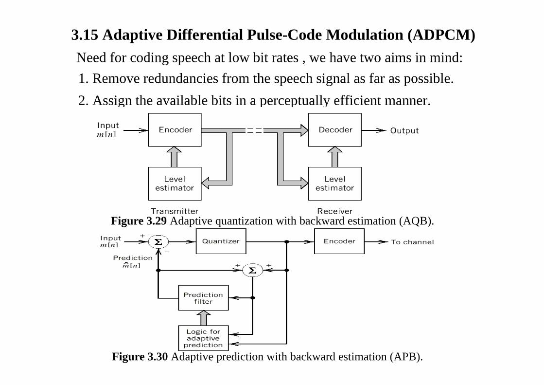
3.15 Adaptive Differential Pulse-Code Modulation (ADPCM)Need for coding speech at low bit rates , we have two aims in mind:Need for coding speech at low bit rates , we have two aims in mind:1. Remove redundancies from the speech signal as far as possible.2. Assign the available bits in a perceptually efficient manner.. ss g e v b e b s pe cep u y e c e e .

Figure 3.29 Adaptive quantization with backward estimation (AQB).

Figure 3.30 Adaptive prediction with backward estimation (APB).

3 1 Introduction 3.1 Introduction Let gδ(

Documents

Transcript of 3 1 Introduction 3.1 Introduction Let gδ(