IntroductionLecture slides for Chapter 1 of Deep Learning

www.deeplearningbook.org Ian Goodfellow

2016-09-26

(Goodfellow 2016)

Representations MatterCHAPTER 1. INTRODUCTION

x

y

Cartesian coordinates

r

θ

Polar coordinates

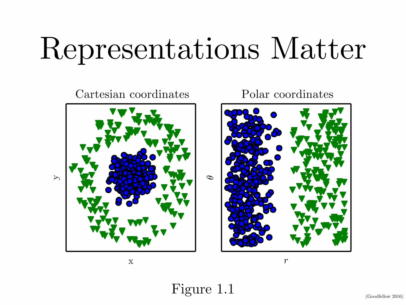
Figure 1.1: Example of different representations: suppose we want to separate twocategories of data by drawing a line between them in a scatterplot. In the plot on the left,we represent some data using Cartesian coordinates, and the task is impossible. In the ploton the right, we represent the data with polar coordinates and the task becomes simple tosolve with a vertical line. Figure produced in collaboration with David Warde-Farley.

One solution to this problem is to use machine learning to discover not onlythe mapping from representation to output but also the representation itself.This approach is known as representation learning. Learned representationsoften result in much better performance than can be obtained with hand-designedrepresentations. They also allow AI systems to rapidly adapt to new tasks, withminimal human intervention. A representation learning algorithm can discover agood set of features for a simple task in minutes, or a complex task in hours tomonths. Manually designing features for a complex task requires a great deal ofhuman time and effort; it can take decades for an entire community of researchers.

The quintessential example of a representation learning algorithm is the au-toencoder. An autoencoder is the combination of an encoder function thatconverts the input data into a different representation, and a decoder functionthat converts the new representation back into the original format. Autoencodersare trained to preserve as much information as possible when an input is runthrough the encoder and then the decoder, but are also trained to make the newrepresentation have various nice properties. Different kinds of autoencoders aim toachieve different kinds of properties.

When designing features or algorithms for learning features, our goal is usuallyto separate the factors of variation that explain the observed data. In thiscontext, we use the word “factors” simply to refer to separate sources of influence;the factors are usually not combined by multiplication. Such factors are often not

4

Figure 1.1

(Goodfellow 2016)

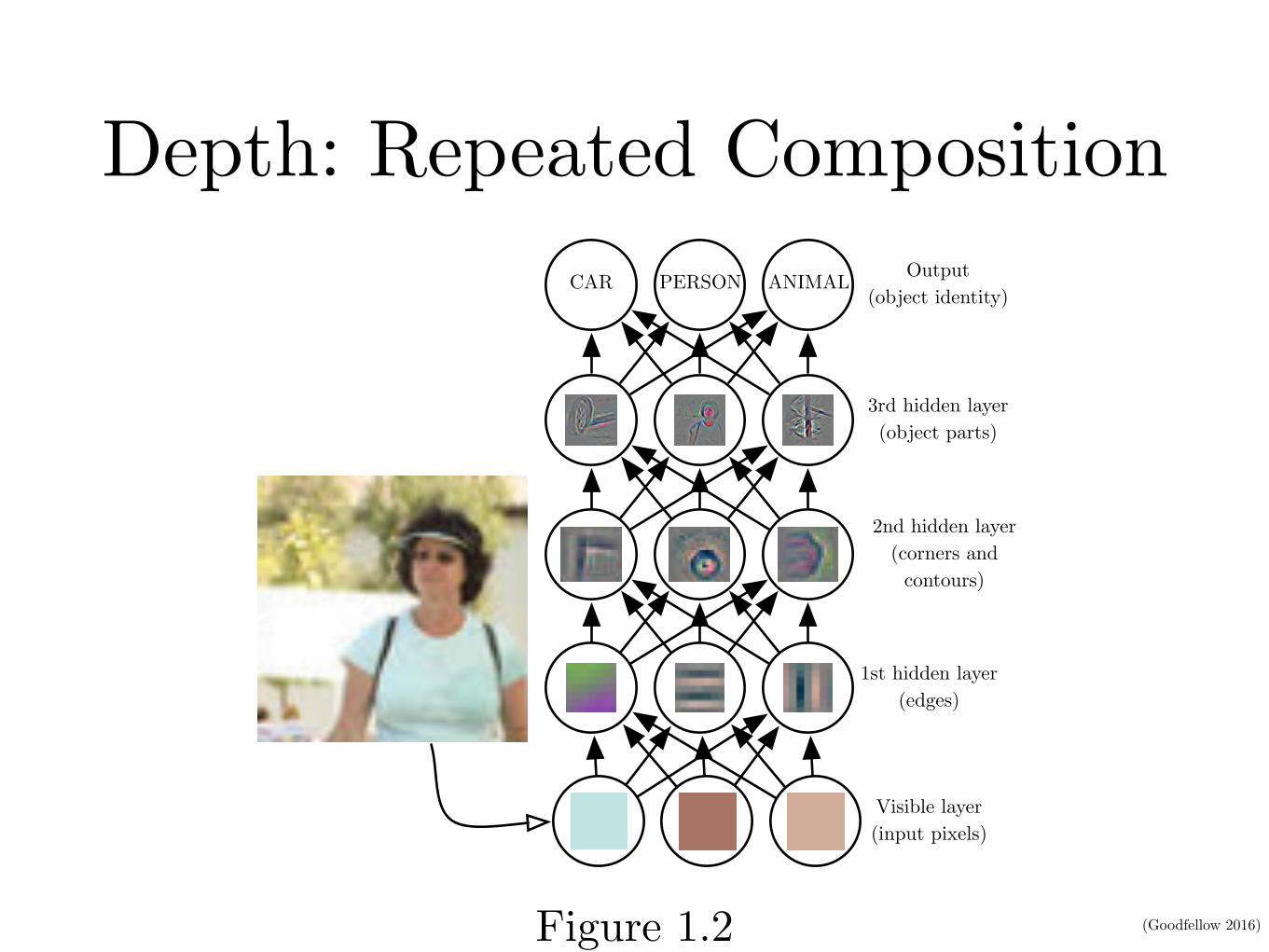
Depth: Repeated CompositionCHAPTER 1. INTRODUCTION

Visible layer(input pixels)

1st hidden layer(edges)

2nd hidden layer(corners and

contours)

3rd hidden layer(object parts)

CAR PERSON ANIMAL Output(object identity)

Figure 1.2: Illustration of a deep learning model. It is difficult for a computer to understandthe meaning of raw sensory input data, such as this image represented as a collectionof pixel values. The function mapping from a set of pixels to an object identity is verycomplicated. Learning or evaluating this mapping seems insurmountable if tackled directly.Deep learning resolves this difficulty by breaking the desired complicated mapping into aseries of nested simple mappings, each described by a different layer of the model. Theinput is presented at the visible layer, so named because it contains the variables thatwe are able to observe. Then a series of hidden layers extracts increasingly abstractfeatures from the image. These layers are called “hidden” because their values are not givenin the data; instead the model must determine which concepts are useful for explainingthe relationships in the observed data. The images here are visualizations of the kindof feature represented by each hidden unit. Given the pixels, the first layer can easilyidentify edges, by comparing the brightness of neighboring pixels. Given the first hiddenlayer’s description of the edges, the second hidden layer can easily search for corners andextended contours, which are recognizable as collections of edges. Given the second hiddenlayer’s description of the image in terms of corners and contours, the third hidden layercan detect entire parts of specific objects, by finding specific collections of contours andcorners. Finally, this description of the image in terms of the object parts it contains canbe used to recognize the objects present in the image. Images reproduced with permissionfrom Zeiler and Fergus (2014).

6

Figure 1.2

(Goodfellow 2016)

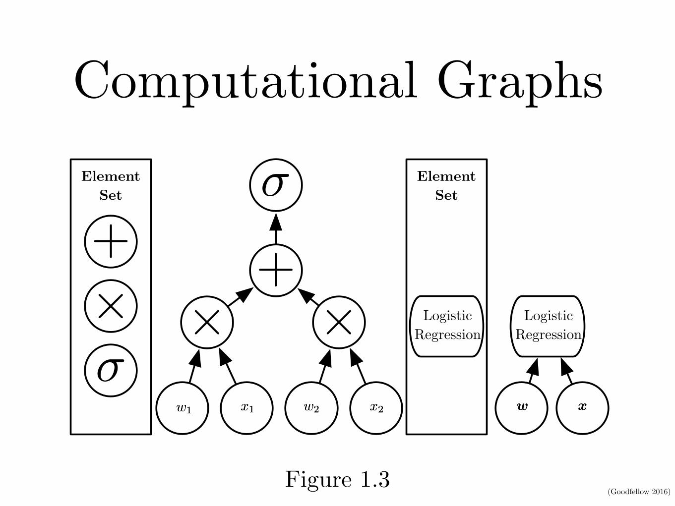
Computational GraphsCHAPTER 1. INTRODUCTION

x1

x1

�

w1

w1

⇥x

2

x2

w2

w2

⇥+

ElementSet

+

⇥�

xxww

ElementSet

LogisticRegression

LogisticRegression

Figure 1.3: Illustration of computational graphs mapping an input to an output whereeach node performs an operation. Depth is the length of the longest path from input tooutput but depends on the definition of what constitutes a possible computational step.The computation depicted in these graphs is the output of a logistic regression model,�(wT x), where � is the logistic sigmoid function. If we use addition, multiplication andlogistic sigmoids as the elements of our computer language, then this model has depththree. If we view logistic regression as an element itself, then this model has depth one.

instructions can refer back to the results of earlier instructions. According to thisview of deep learning, not all of the information in a layer’s activations necessarilyencodes factors of variation that explain the input. The representation also storesstate information that helps to execute a program that can make sense of the input.This state information could be analogous to a counter or pointer in a traditionalcomputer program. It has nothing to do with the content of the input specifically,but it helps the model to organize its processing.

There are two main ways of measuring the depth of a model. The first view isbased on the number of sequential instructions that must be executed to evaluatethe architecture. We can think of this as the length of the longest path througha flow chart that describes how to compute each of the model’s outputs givenits inputs. Just as two equivalent computer programs will have different lengthsdepending on which language the program is written in, the same function maybe drawn as a flowchart with different depths depending on which functions weallow to be used as individual steps in the flowchart. Figure 1.3 illustrates how thischoice of language can give two different measurements for the same architecture.

Another approach, used by deep probabilistic models, regards the depth of amodel as being not the depth of the computational graph but the depth of thegraph describing how concepts are related to each other. In this case, the depth

7

Figure 1.3

(Goodfellow 2016)

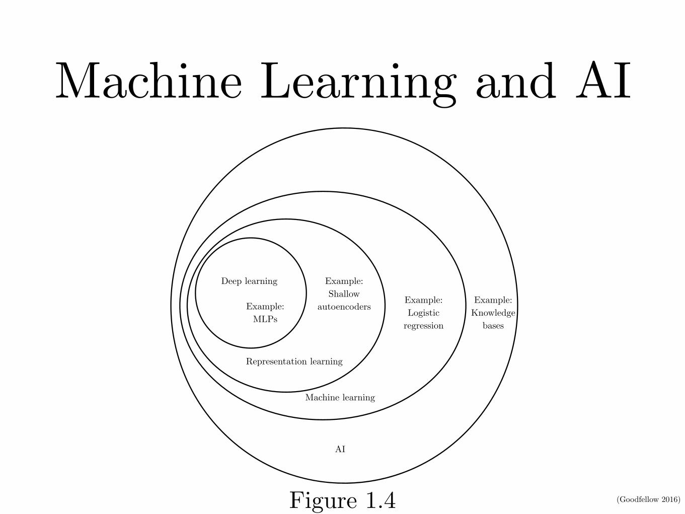
Machine Learning and AI

CHAPTER 1. INTRODUCTION

AI

Machine learning

Representation learning

Deep learning

Example:Knowledge

bases

Example:Logistic

regression

Example:Shallow

autoencodersExample:MLPs

Figure 1.4: A Venn diagram showing how deep learning is a kind of representation learning,which is in turn a kind of machine learning, which is used for many but not all approachesto AI. Each section of the Venn diagram includes an example of an AI technology.

9

Figure 1.4

(Goodfellow 2016)

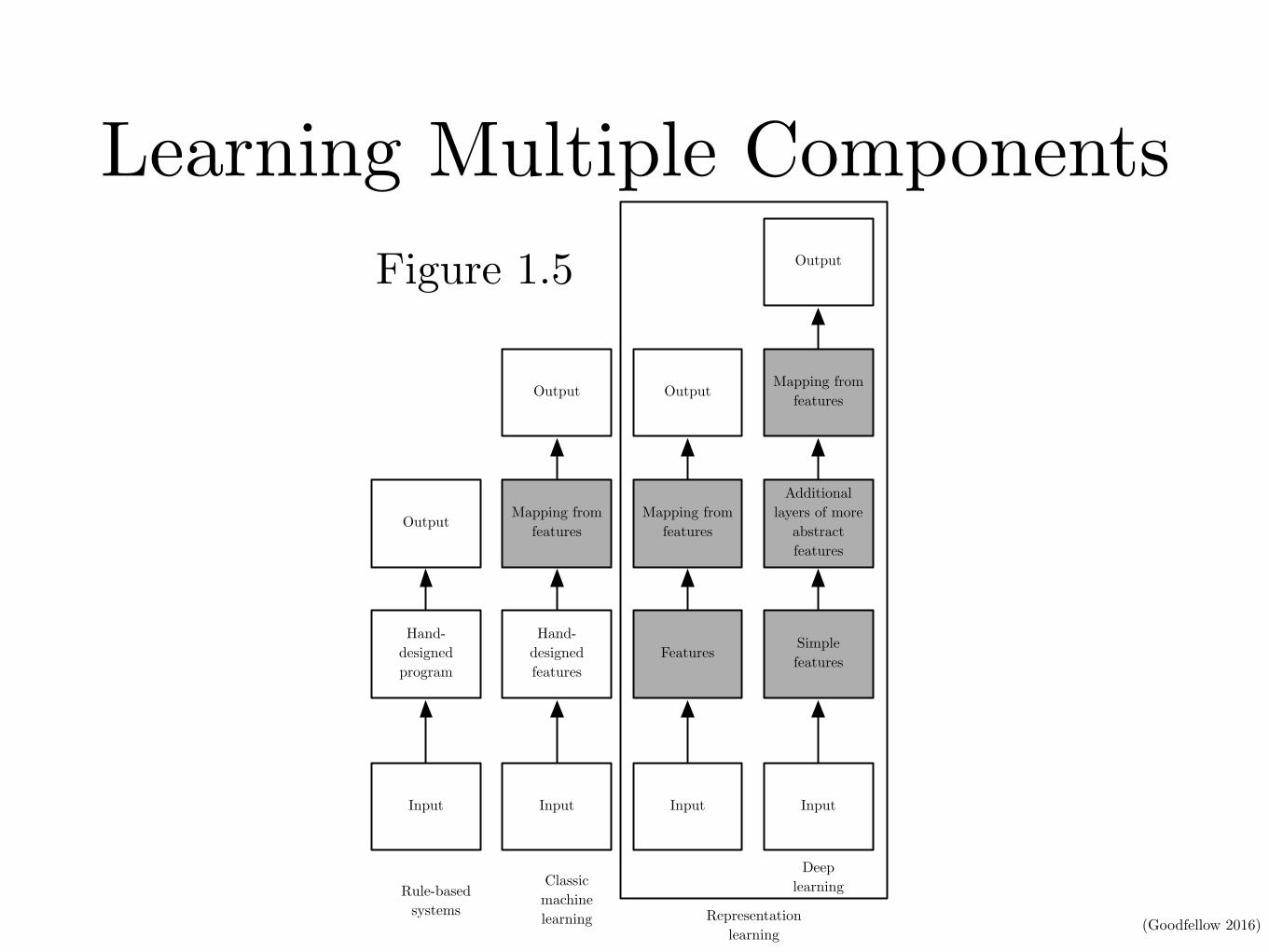
Learning Multiple ComponentsCHAPTER 1. INTRODUCTION

Input

Hand-designed program

Output

Input

Hand-designed features

Mapping from features

Output

Input

Features

Mapping from features

Output

Input

Simple features

Mapping from features

Output

Additional layers of more

abstract features

Rule-basedsystems

Classicmachinelearning Representation

learning

Deeplearning

Figure 1.5: Flowcharts showing how the different parts of an AI system relate to eachother within different AI disciplines. Shaded boxes indicate components that are able tolearn from data.

10

Figure 1.5

(Goodfellow 2016)

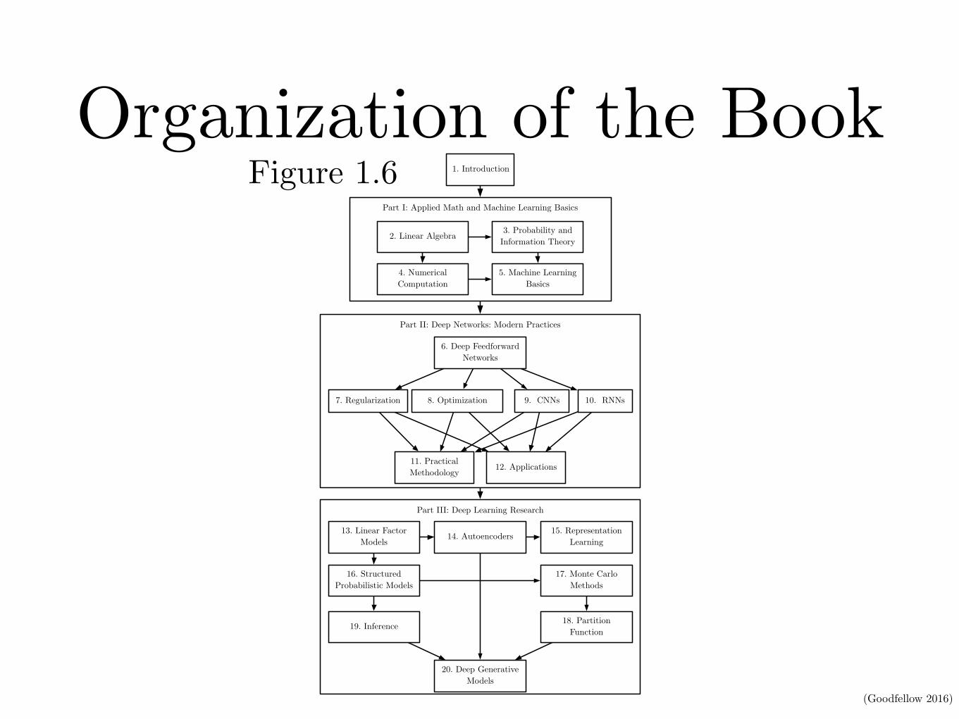
Organization of the BookCHAPTER 1. INTRODUCTION

1. Introduction

Part I: Applied Math and Machine Learning Basics

2. Linear Algebra 3. Probability and Information Theory

4. Numerical Computation

5. Machine Learning Basics

Part II: Deep Networks: Modern Practices

6. Deep Feedforward Networks

7. Regularization 8. Optimization 9. CNNs 10. RNNs

11. Practical Methodology 12. Applications

Part III: Deep Learning Research

13. Linear Factor Models 14. Autoencoders 15. Representation

Learning

16. Structured Probabilistic Models

17. Monte Carlo Methods

18. Partition Function19. Inference

20. Deep Generative Models

Figure 1.6: The high-level organization of the book. An arrow from one chapter to anotherindicates that the former chapter is prerequisite material for understanding the latter.

12

Figure 1.6

(Goodfellow 2016)

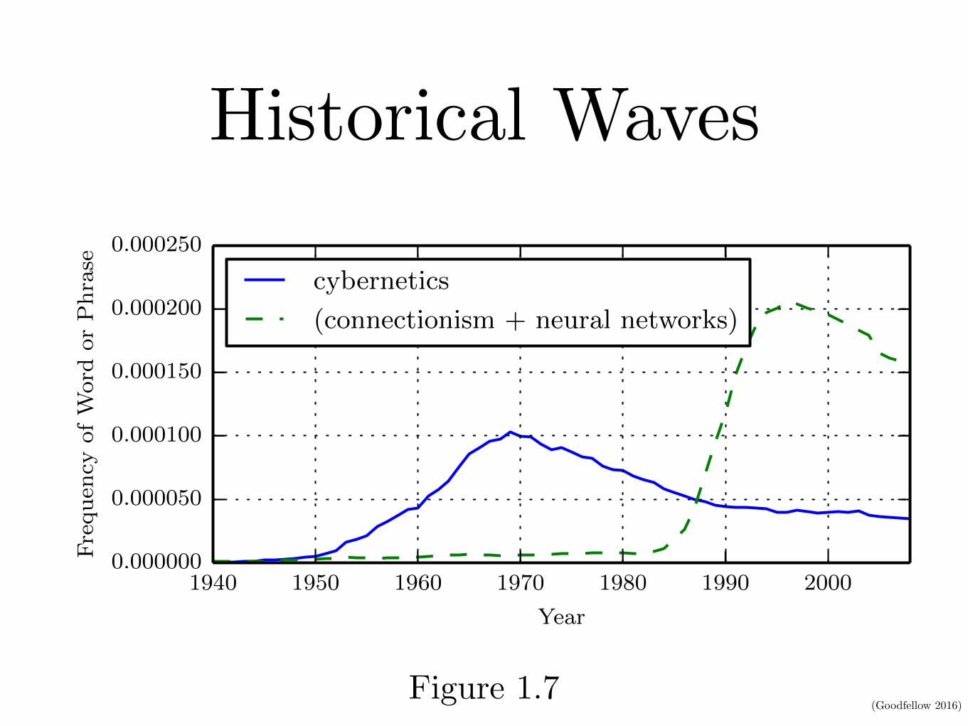
Historical Waves

CHAPTER 1. INTRODUCTION

1940 1950 1960 1970 1980 1990 2000

Year

0.000000

0.000050

0.000100

0.000150

0.000200

0.000250

Frequency

ofW

ord

or

Phrase

cybernetics

(connectionism + neural networks)

Figure 1.7: The figure shows two of the three historical waves of artificial neural netsresearch, as measured by the frequency of the phrases “cybernetics” and “connectionism” or“neural networks” according to Google Books (the third wave is too recent to appear). Thefirst wave started with cybernetics in the 1940s–1960s, with the development of theoriesof biological learning (McCulloch and Pitts, 1943; Hebb, 1949) and implementations ofthe first models such as the perceptron (Rosenblatt, 1958) allowing the training of a singleneuron. The second wave started with the connectionist approach of the 1980–1995 period,with back-propagation (Rumelhart et al., 1986a) to train a neural network with one or twohidden layers. The current and third wave, deep learning, started around 2006 (Hintonet al., 2006; Bengio et al., 2007; Ranzato et al., 2007a), and is just now appearing in bookform as of 2016. The other two waves similarly appeared in book form much later thanthe corresponding scientific activity occurred.

14

Figure 1.7

(Goodfellow 2016)

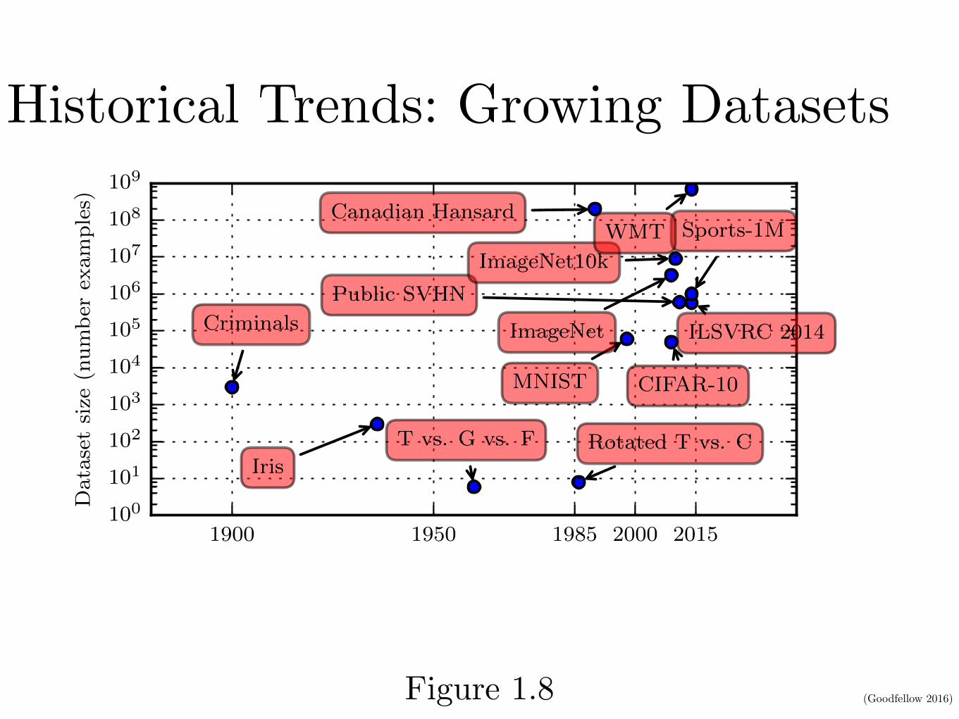
Historical Trends: Growing Datasets

CHAPTER 1. INTRODUCTION

1900 1950 1985 2000 2015

Year

10

0

10

1

10

2

10

3

10

4

10

5

10

6

10

7

10

8

10

9

Dataset

size

(num

ber

exam

ples)

Iris

MNIST

Public SVHN

ImageNet

CIFAR-10

ImageNet10k

ILSVRC 2014

Sports-1M

Rotated T vs. C

T vs. G vs. F

Criminals

Canadian Hansard

WMT

Figure 1.8: Dataset sizes have increased greatly over time. In the early 1900s, statisticiansstudied datasets using hundreds or thousands of manually compiled measurements (Garson,1900; Gosset, 1908; Anderson, 1935; Fisher, 1936). In the 1950s through 1980s, the pioneersof biologically inspired machine learning often worked with small, synthetic datasets, suchas low-resolution bitmaps of letters, that were designed to incur low computational cost anddemonstrate that neural networks were able to learn specific kinds of functions (Widrowand Hoff, 1960; Rumelhart et al., 1986b). In the 1980s and 1990s, machine learningbecame more statistical in nature and began to leverage larger datasets containing tensof thousands of examples such as the MNIST dataset (shown in figure 1.9) of scansof handwritten numbers (LeCun et al., 1998b). In the first decade of the 2000s, moresophisticated datasets of this same size, such as the CIFAR-10 dataset (Krizhevsky andHinton, 2009) continued to be produced. Toward the end of that decade and throughoutthe first half of the 2010s, significantly larger datasets, containing hundreds of thousandsto tens of millions of examples, completely changed what was possible with deep learning.These datasets included the public Street View House Numbers dataset (Netzer et al.,2011), various versions of the ImageNet dataset (Deng et al., 2009, 2010a; Russakovskyet al., 2014a), and the Sports-1M dataset (Karpathy et al., 2014). At the top of thegraph, we see that datasets of translated sentences, such as IBM’s dataset constructedfrom the Canadian Hansard (Brown et al., 1990) and the WMT 2014 English to Frenchdataset (Schwenk, 2014) are typically far ahead of other dataset sizes.

21

Figure 1.8

(Goodfellow 2016)

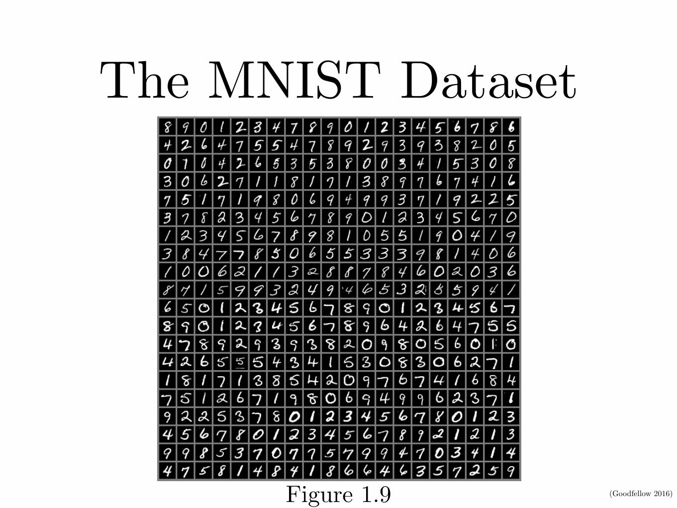
The MNIST DatasetCHAPTER 1. INTRODUCTION

Figure 1.9: Example inputs from the MNIST dataset. The “NIST” stands for NationalInstitute of Standards and Technology, the agency that originally collected this data.The “M” stands for “modified,” since the data has been preprocessed for easier use withmachine learning algorithms. The MNIST dataset consists of scans of handwritten digitsand associated labels describing which digit 0–9 is contained in each image. This simpleclassification problem is one of the simplest and most widely used tests in deep learningresearch. It remains popular despite being quite easy for modern techniques to solve.Geoffrey Hinton has described it as “the drosophila of machine learning,” meaning thatit allows machine learning researchers to study their algorithms in controlled laboratoryconditions, much as biologists often study fruit flies.

22

Figure 1.9

(Goodfellow 2016)

Connections per Neuron

CHAPTER 1. INTRODUCTION

1950 1985 2000 2015

Year

10

1

10

2

10

3

10

4

Connections

per

neuron

1

2

3

4

5

6

7

8

9

10

Fruit fly

Mouse

Cat

Human

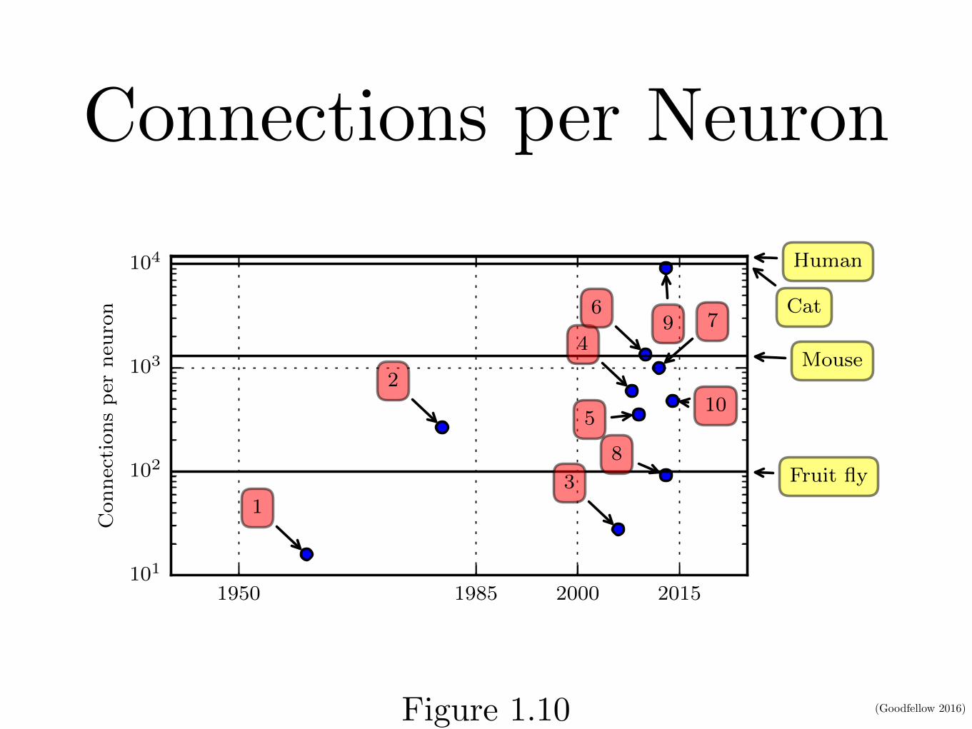
Figure 1.10: Initially, the number of connections between neurons in artificial neuralnetworks was limited by hardware capabilities. Today, the number of connections betweenneurons is mostly a design consideration. Some artificial neural networks have nearly asmany connections per neuron as a cat, and it is quite common for other neural networksto have as many connections per neuron as smaller mammals like mice. Even the humanbrain does not have an exorbitant amount of connections per neuron. Biological neuralnetwork sizes from Wikipedia (2015).

1. Adaptive linear element (Widrow and Hoff, 1960)

2. Neocognitron (Fukushima, 1980)

3. GPU-accelerated convolutional network (Chellapilla et al., 2006)

4. Deep Boltzmann machine (Salakhutdinov and Hinton, 2009a)

5. Unsupervised convolutional network (Jarrett et al., 2009)

6. GPU-accelerated multilayer perceptron (Ciresan et al., 2010)

7. Distributed autoencoder (Le et al., 2012)

8. Multi-GPU convolutional network (Krizhevsky et al., 2012)

9. COTS HPC unsupervised convolutional network (Coates et al., 2013)

10. GoogLeNet (Szegedy et al., 2014a)

24

Figure 1.10

(Goodfellow 2016)

Number of Neurons

CHAPTER 1. INTRODUCTION

1950 1985 2000 2015 2056

Year

10

�2

10

�1

10

0

10

1

10

2

10

3

10

4

10

5

10

6

10

7

10

8

10

9

10

10

10

11

Num

ber

ofneurons

(logarithm

ic

scale)

1

2

3

4

5

6

7

8

9

10

11

12

13

14

15

16

17

18

19

20

Sponge

Roundworm

Leech

Ant

Bee

Frog

Octopus

Human

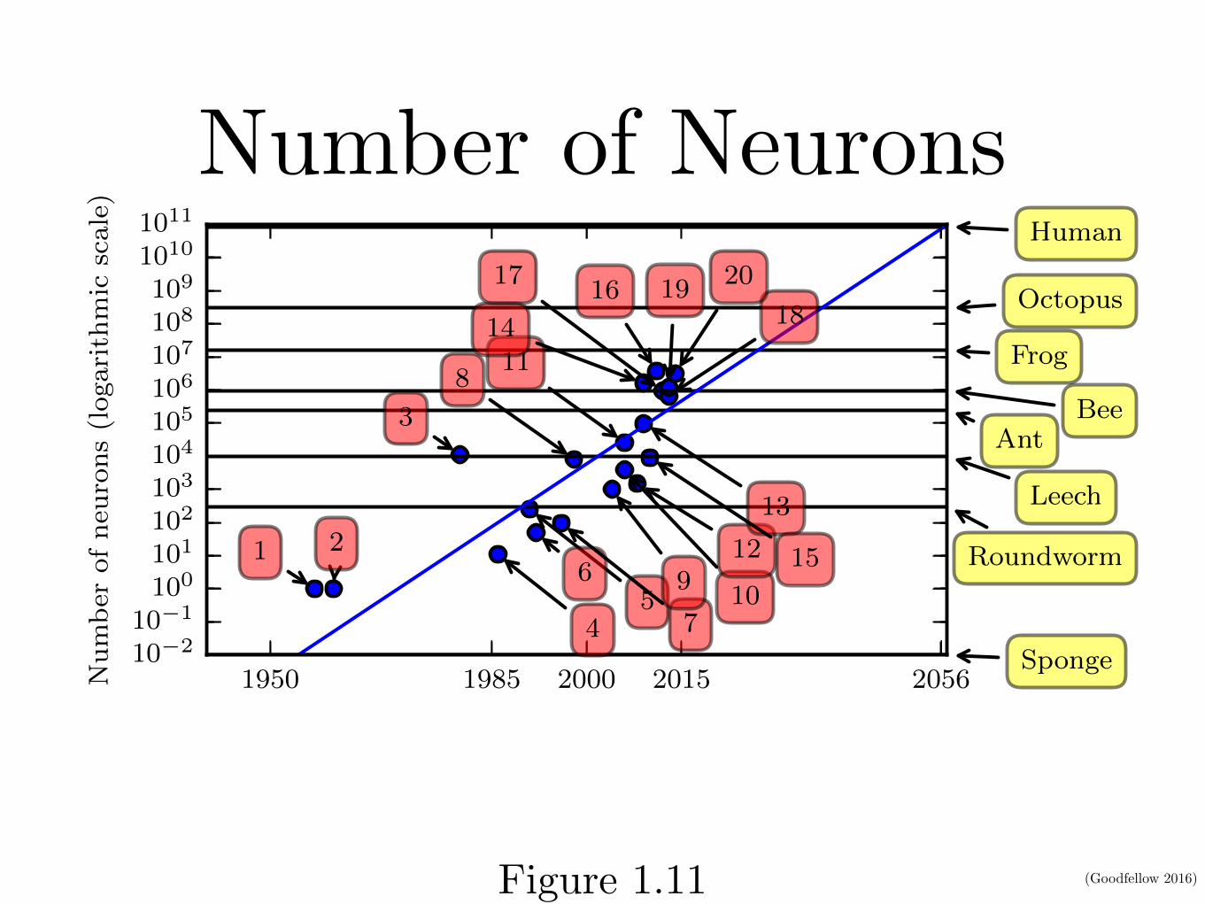
Figure 1.11: Since the introduction of hidden units, artificial neural networks have doubledin size roughly every 2.4 years. Biological neural network sizes from Wikipedia (2015).

1. Perceptron (Rosenblatt, 1958, 1962)

2. Adaptive linear element (Widrow and Hoff, 1960)

3. Neocognitron (Fukushima, 1980)

4. Early back-propagation network (Rumelhart et al., 1986b)

5. Recurrent neural network for speech recognition (Robinson and Fallside, 1991)

6. Multilayer perceptron for speech recognition (Bengio et al., 1991)

7. Mean field sigmoid belief network (Saul et al., 1996)

8. LeNet-5 (LeCun et al., 1998b)

9. Echo state network (Jaeger and Haas, 2004)

10. Deep belief network (Hinton et al., 2006)

11. GPU-accelerated convolutional network (Chellapilla et al., 2006)

12. Deep Boltzmann machine (Salakhutdinov and Hinton, 2009a)

13. GPU-accelerated deep belief network (Raina et al., 2009)

14. Unsupervised convolutional network (Jarrett et al., 2009)

15. GPU-accelerated multilayer perceptron (Ciresan et al., 2010)

16. OMP-1 network (Coates and Ng, 2011)

17. Distributed autoencoder (Le et al., 2012)

18. Multi-GPU convolutional network (Krizhevsky et al., 2012)

19. COTS HPC unsupervised convolutional network (Coates et al., 2013)

20. GoogLeNet (Szegedy et al., 2014a)

27

Figure 1.11

(Goodfellow 2016)

Solving Object Recognition

CHAPTER 1. INTRODUCTION

2010 2011 2012 2013 2014 2015

Year

0.00

0.05

0.10

0.15

0.20

0.25

0.30

ILSV

RC

classification

error

rate

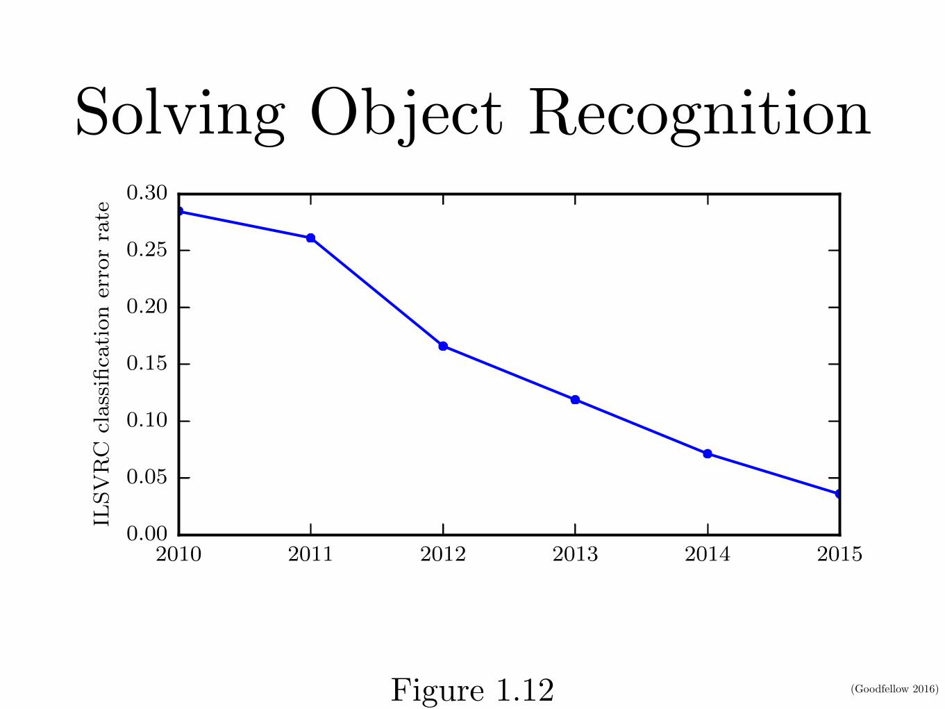
Figure 1.12: Since deep networks reached the scale necessary to compete in the ImageNetLarge Scale Visual Recognition Challenge, they have consistently won the competitionevery year, and yielded lower and lower error rates each time. Data from Russakovskyet al. (2014b) and He et al. (2015).

28

Figure 1.12