Image-Based Aspect Ratio...
10
Image-Based Aspect Ratio Selection Yunhai Wang, Zeyu Wang, Chi-Wing Fu, Hansj¨ org Schmauder, Oliver Deussen and Daniel Weiskopf Fig. 1. Influence of aspect ratio α on the perception of trends and cluster separability for the Sunspot dataset [21] (a, b, c) and the Contraceptive Method Choice (CMC) dataset [10] (d, e). (a) Line chart with the default aspect ratio, and (b) the aspect ratio selected by an existing method (RV) [40], where both methods obscure the trends over the cycles. (c) The aspect ratio selected by our method (imgRV), where detailed cycle oscillations are revealed. (d) Scatter plot of three data clusters with the default aspect ratio, where the visual separation between the two clusters on the left is unclear. (e) The aspect ratio selected by our method shows clearer cluster structures. Abstract—Selecting a good aspect ratio is crucial for effective 2D diagrams. There are several aspect ratio selection methods for function plots and line charts, but only few can handle general, discrete diagrams such as 2D scatter plots. However, these methods either lack a perceptual foundation or heavily rely on intermediate isoline representations, which depend on choosing the right isovalues and are time-consuming to compute. This paper introduces a general image-based approach for selecting aspect ratios for a wide variety of 2D diagrams, ranging from scatter plots and density function plots to line charts. Our approach is derived from Federer’s co-area formula and a line integral representation that enable us to directly construct image-based versions of existing selection methods using density fields. In contrast to previous methods, our approach bypasses isoline computation, so it is faster to compute, while following the perceptual foundation to select aspect ratios. Furthermore, this approach is complemented by an anisotropic kernel density estimation to construct density fields, allowing us to more faithfully characterize data patterns, such as the subgroups in scatterplots or dense regions in time series. We demonstrate the effectiveness of our approach by quantitatively comparing to previous methods and revisiting a prior user study. Finally, we present extensions for ROI banking, multi-scale banking, and the application to image data. Index Terms—Aspect ratio, image-based method, Federer’s co-area formula, density field, anisotropic kernel density estimation. 1 I NTRODUCTION Visual attributes like size, shape, and slope greatly influence the ex- pressiveness and effectiveness of a visualization [25]. In particular, the aspect ratio (defined as the fraction, height/width, throughout the paper) has a dramatic effect on the perception of data patterns in a visualization [6]. A well-chosen aspect ratio may reveal trends and relevant clusters that are hidden by a bad aspect ratio. Figure 1 demonstrates the influence of the aspect ratio. An improper aspect ratio obscures the oscillations over the cycles (Figure 1 (a, b)) and leads to a poor visual cluster separation (Figure 1 (d)). In contrast, an appropriate aspect ratio attempts to reveal major patterns as much • Y. Wang and Z. Wang are with Shandong University. Email: {cloudseawang,zywangx}@gmail.com. Y. Wang and Z. Wang are joint first authors. • C.-W. Fu is with the Chinese University of Hong Kong. E-mail: [email protected]. • O. Deussen is with Konstanz University, Germany and Shenzhen VisuCA Key Lab, SIAT, China. E-mail: [email protected]. • H. Schmauder and D. Weiskopf are with VISUS, University of Stuttgart, Germany. E-mail: {hansjoerg.schmauder, Daniel.Weiskopf}@visus. uni-stuttgart.de. Manuscript received xx xxx. 201x; accepted xx xxx. 201x. Date of Publication xx xxx. 201x; date of current version xx xxx. 201x. For information on obtaining reprints of this article, please send e-mail to: [email protected]. Digital Object Identifier: xx.xxxx/TVCG.201x.xxxxxxx as possible (Figure 1 (c, e)). Therefore, methods for automatically choosing a proper aspect ratio for a given visualization are of high interest for a broad range of visualizations and applications. Selecting appropriate aspect ratios for 2D line charts has been well studied. Cleveland et al. [8] pioneered the principle of banking to 45 ◦ and proposed two methods: average absolute orientation (AO) and arc length weighted average absolute orientation (AWO). Both methods select aspect ratios by banking the orientation of a line chart’s line segments at around 45 degrees. AWO generally produces reasonable aspect ratios for most data. Guha and Cleveland [29] and Talbot et al. [34] suggested two alternative approaches: the resultant vector (RV) and arc length based (AL) methods, based on geometric measures such as the resultant vector and the curve’s arc length, respectively. Recent work [40] showed that both methods tend to satisfy the banking to 45 ◦ principle and select almost the same aspect ratio as AWO, while RV is usually faster and more robust. However, all aforementioned methods are specifically designed for line charts and cannot handle other common 2D visualizations such as scatter plots. To facilitate scatter plots, Fink et al. [16] selected aspect ratios based on a Delaunay triangulation [16]. Various geometric criteria were employed, e.g., large minimum angle and total edge length. However, due to the lack of a perceptual foundation, aspect ratios selected by this method might not be favoured by users for certain datasets. Moreover, it is relatively slow; as reported in the paper, it requires several minutes to compute the aspect ratio for a scatter plot with 1,000 points. Talbot et al. [34] proposed an isoline-based approach to selecting aspect ratios by applying existing methods to 2D isolines extracted from the density field derived from a scatter plot. This method
Transcript of Image-Based Aspect Ratio...
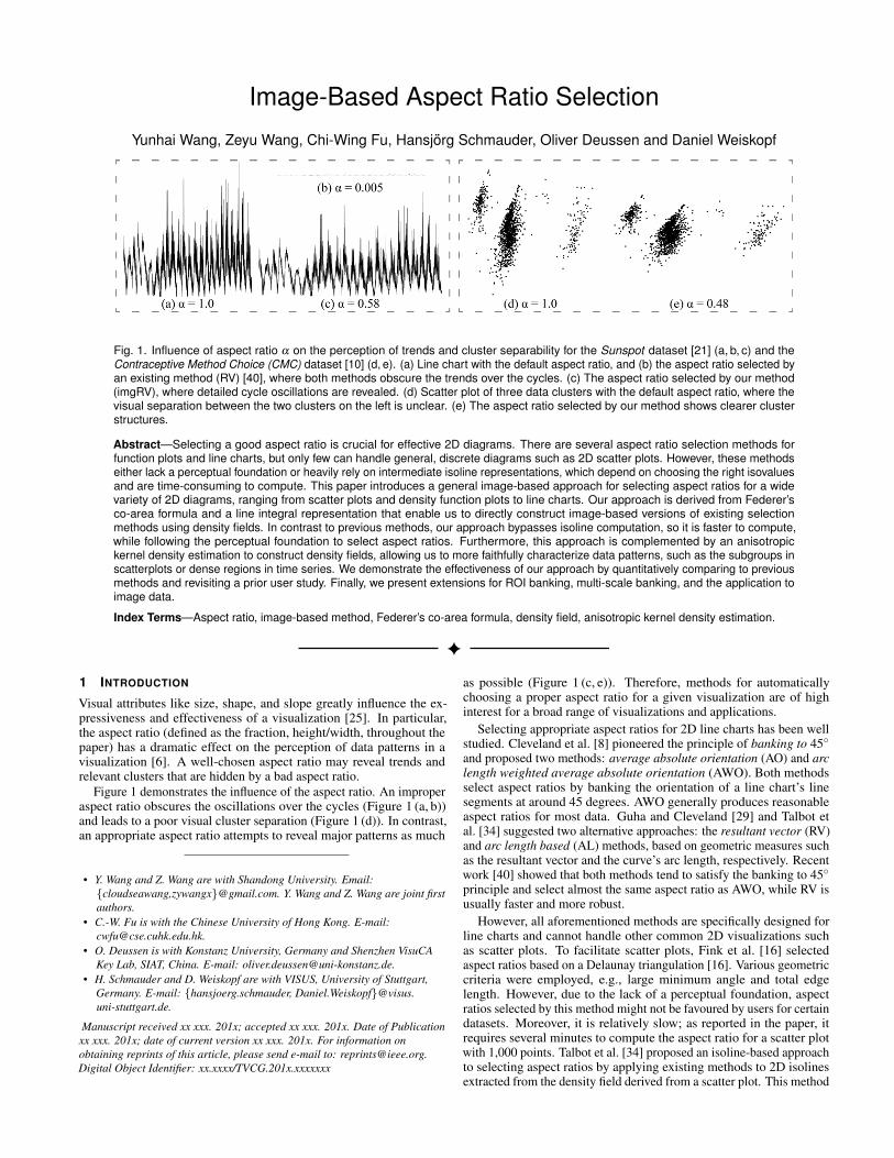
Image-Based Aspect Ratio Selection
Yunhai Wang, Zeyu Wang, Chi-Wing Fu, Hansjorg Schmauder, Oliver Deussen and Daniel Weiskopf
Fig. 1. Influence of aspect ratio α on the perception of trends and cluster separability for the Sunspot dataset [21] (a, b, c) and theContraceptive Method Choice (CMC) dataset [10] (d, e). (a) Line chart with the default aspect ratio, and (b) the aspect ratio selected byan existing method (RV) [40], where both methods obscure the trends over the cycles. (c) The aspect ratio selected by our method(imgRV), where detailed cycle oscillations are revealed. (d) Scatter plot of three data clusters with the default aspect ratio, where thevisual separation between the two clusters on the left is unclear. (e) The aspect ratio selected by our method shows clearer clusterstructures.
Abstract—Selecting a good aspect ratio is crucial for effective 2D diagrams. There are several aspect ratio selection methods forfunction plots and line charts, but only few can handle general, discrete diagrams such as 2D scatter plots. However, these methodseither lack a perceptual foundation or heavily rely on intermediate isoline representations, which depend on choosing the right isovaluesand are time-consuming to compute. This paper introduces a general image-based approach for selecting aspect ratios for a widevariety of 2D diagrams, ranging from scatter plots and density function plots to line charts. Our approach is derived from Federer’sco-area formula and a line integral representation that enable us to directly construct image-based versions of existing selectionmethods using density fields. In contrast to previous methods, our approach bypasses isoline computation, so it is faster to compute,while following the perceptual foundation to select aspect ratios. Furthermore, this approach is complemented by an anisotropickernel density estimation to construct density fields, allowing us to more faithfully characterize data patterns, such as the subgroups inscatterplots or dense regions in time series. We demonstrate the effectiveness of our approach by quantitatively comparing to previousmethods and revisiting a prior user study. Finally, we present extensions for ROI banking, multi-scale banking, and the application toimage data.
Index Terms—Aspect ratio, image-based method, Federer’s co-area formula, density field, anisotropic kernel density estimation.
1 INTRODUCTION
Visual attributes like size, shape, and slope greatly influence the ex-pressiveness and effectiveness of a visualization [25]. In particular,the aspect ratio (defined as the fraction, height/width, throughout thepaper) has a dramatic effect on the perception of data patterns in avisualization [6]. A well-chosen aspect ratio may reveal trends andrelevant clusters that are hidden by a bad aspect ratio.
Figure 1 demonstrates the influence of the aspect ratio. An improperaspect ratio obscures the oscillations over the cycles (Figure 1 (a, b))and leads to a poor visual cluster separation (Figure 1 (d)). In contrast,an appropriate aspect ratio attempts to reveal major patterns as much
• Y. Wang and Z. Wang are with Shandong University. Email:cloudseawang,[email protected]. Y. Wang and Z. Wang are joint firstauthors.
• C.-W. Fu is with the Chinese University of Hong Kong. E-mail:[email protected].
• O. Deussen is with Konstanz University, Germany and Shenzhen VisuCAKey Lab, SIAT, China. E-mail: [email protected].
• H. Schmauder and D. Weiskopf are with VISUS, University of Stuttgart,Germany. E-mail: hansjoerg.schmauder, [email protected].
Manuscript received xx xxx. 201x; accepted xx xxx. 201x. Date of Publicationxx xxx. 201x; date of current version xx xxx. 201x. For information onobtaining reprints of this article, please send e-mail to: [email protected] Object Identifier: xx.xxxx/TVCG.201x.xxxxxxx
as possible (Figure 1 (c, e)). Therefore, methods for automaticallychoosing a proper aspect ratio for a given visualization are of highinterest for a broad range of visualizations and applications.
Selecting appropriate aspect ratios for 2D line charts has been wellstudied. Cleveland et al. [8] pioneered the principle of banking to 45and proposed two methods: average absolute orientation (AO) and arclength weighted average absolute orientation (AWO). Both methodsselect aspect ratios by banking the orientation of a line chart’s linesegments at around 45 degrees. AWO generally produces reasonableaspect ratios for most data. Guha and Cleveland [29] and Talbot etal. [34] suggested two alternative approaches: the resultant vector (RV)and arc length based (AL) methods, based on geometric measures suchas the resultant vector and the curve’s arc length, respectively. Recentwork [40] showed that both methods tend to satisfy the banking to 45principle and select almost the same aspect ratio as AWO, while RV isusually faster and more robust.
However, all aforementioned methods are specifically designed forline charts and cannot handle other common 2D visualizations suchas scatter plots. To facilitate scatter plots, Fink et al. [16] selectedaspect ratios based on a Delaunay triangulation [16]. Various geometriccriteria were employed, e.g., large minimum angle and total edgelength. However, due to the lack of a perceptual foundation, aspectratios selected by this method might not be favoured by users for certaindatasets. Moreover, it is relatively slow; as reported in the paper, itrequires several minutes to compute the aspect ratio for a scatter plotwith 1,000 points. Talbot et al. [34] proposed an isoline-based approachto selecting aspect ratios by applying existing methods to 2D isolinesextracted from the density field derived from a scatter plot. This method
can find proper aspect ratios for most data; however, it depends on (i) thenumber of isolines extracted from the density field and (ii) the qualityof the density field constructed from the data. Insufficient isolines oran improper kernel for estimating the density field [33] might result inundesirable aspect ratios that obscure patterns in the data.
In this paper, we present a generalized image-based approach forfinding aspect ratios for 2D diagrams such as scatter plots, densityfunction plots, and line charts. If the input data is not given in the formof a density field but as discrete geometric points, we construct sucha field by kernel density estimation (KDE) with Gaussian kernels. Incontrast to previous methods, our approach works directly with densityfields defined over 2D visualizations without the need to generateintermediate data such as the isolines; see Figure 2. We formulateour approach based on Federer’s co-area formula [14] in geometricmeasure theory to transform line integrals over sets of isolines of thedensity field to area integrals over the density field itself. Using ourformulation, previous methods that can be rewritten as line integralscan be extended to work directly with density fields. In addition, tofaithfully characterize data patterns, we introduce anisotropic KDE toconstruct the density fields, where the kernel associated with each datapoint adapts to the local structure around the point.
Compared to conventional isoline-based approaches, our methodalso follows the principle of banking to 45, but it avoids discreteisolines as intermediate data and works directly with the density fields.Hence, it achieves an accurate and fast computation. Since densityfields are often continuous and even smooth, directly computing theaspect ratios from them avoids the limitations of existing methods,e.g., they cannot handle data with spike noise [40] (see Figure 1 (b)).Moreover, our approach is not limited to using a density field of adiscrete visualization but can be applied to any non-negative and un-normalized field. Hence, we refer to our approach as an image-basedapproach, and thus, it not only encompasses cases that can be handledby the previous methods, but can also be applied more broadly tocontinuous scatter plots and even to 2D images in general.
As shown by Wang et al. [40], AWO, AL, and RV can be formulatedusing line integrals; hence, they can be extended to work directly withdensity fields. Comparing our image-based versions of these methodswith previous isoline-based versions with a large number of isolines,we recommend our method, image-based RV (imgRV), as the defaultaspect ratio selection method, since it produces results similar to mostof the other methods but is the fastest and the most robust. We revisitexamples and the user study by Fink et al. [16] and show that choicesmade by our method are mostly consistent with user preferences.
Last, we show three extensions of our method including region-of-interest (ROI) banking, multi-scale banking, and using images as aninput. We summarize the main contributions of our paper below.
• We present a new aspect ratio selection approach that worksdirectly with density fields constructed from a broad range of 2Dvisualizations. Three image-based aspect ratio selection methodsare formulated by extending the line integral forms of existingmethods AWO, AL, and RV.
• We introduce anisotropic kernels to better characterize the localstructures in the data visualizations.
• We provide a comprehensive evaluation of a variety of methods,showing that the results of our image-based methods and isoline-based methods converge, but our methods are about an order ofmagnitude faster than existing methods.
2 RELATED WORK
Bertin, in his seminal work on the semiotics of graphics [2], alreadypointed out the importance of a proper aspect ratio for the perceptionand readability of diagrams. Hereafter, this influence was studied fordecades, especially for widely-used visualization techniques such asline charts and scatter plots. A number of approaches for the automaticselection of aspect ratios were developed for these techniques.
Banking methods for line charts. Cleveland et al. [8] were the firstto systematically study how the aspect ratio influences the perception
of line charts. Their user studies show that judging the slope ratio be-tween two adjacent line segments is most accurate when the orientationresolution (range of orientations of the two involved line segments) ismaximized. They also showed that maximizing the orientation reso-lution is equivalent to centering the absolute value of the mid-angle(average orientation) at 45. This is known as the banking to 45 prin-ciple, which is the foundation of most aspect ratio selection methods.More recent work by Talbot et al. [35] found that the ability to estimateslopes is sub-optimal when the mid-angle is 45. Nevertheless, mostexisting methods still focus on optimizing for an aspect ratio that bankslines in the visualization to 45.
Based on the 45 principle, Cleveland et al. [5–7] and various otherresearchers developed a number of aspect ratio selection methods, in-cluding median absolute slope (MS), average absolute slope (AS),average absolute orientation (AO), and arc length weighted averageabsolute orientation (AWO). All these methods attempt to center theslopes (or orientations) of line segments around a value of one (or45). MS and AS bank the median and average absolute slope of linesegments to one, whereas AO and AWO bank the average absoluteorientations to 45. AWO weights the average absolute orientation bythe lengths of the line segments; doing so it produces more satisfactoryresults for most cases [7]. Heer and Agrawala [19] developed twomethods to directly compute the orientation resolution: global orienta-tion resolution (GOR) and local orientation resolution (LOR). SinceGOR considers all pairs of line segments in a plot, it is usually slow,whereas LOR considers only successive pairs of line segments, so itis much faster, but it tends to select aspect ratios that are excessivelylarge or small. By using an L1 norm in LOR, L1-LOR [40] was foundto produce more reasonable aspect ratios for most data.
Rather than following the 45 principle, Guha and Cleveland [29]suggested the resultant vector (RV) method, which banks the RV of aline plot to one. RV is the ratio of the total variation of line segmentsin y and x direction. Though its perceptual foundation is not clear,the method produces good results. Similar to RV, the arc length based(AL) [34] method is also not based on the 45 principle; it selects the as-pect ratio by minimizing the arc length of a line chart. Talbot et al. [34]showed that RV can be interpreted as AL using the Manhattan distancemetric, and thus, both methods share several empirical advantagessuch as parameterization invariance, robustness, and low computationalcosts. Recently, Wang et al. [40] showed parameterization invarianceof AL, RV, and AWO using line integrals, and proved that RV and ALtend to satisfy the 45 principle. Through a systematic evaluation ofmost aspect ratio selection methods, they showed that RV and L1-LORhave complementary properties for revealing different data patterns ofinterest, and thus, they proposed a dual-scale banking method that takesadvantages of RV and L1-LOR.
Banking methods for scatter plots. The aspect ratio selection meth-ods above can only handle 1D functions presented as line charts. How-ever, the 2D data may not be represented as a 1D function in general,e.g., 2D distributions of data samples, 2D scatter plots, as well as manyother common forms of 2D visualizations.
For such visualizations, a number of banking methods have beenproposed. From a perceptual point of view, banking ellipse-shapedclusters to circles seems to be a preferable solution [38], since ellipseshave an orientation, which may interfere with the perception of theclusters [11, 24]. Cleveland et al. [6] fitted continuous LOESS curves(local polynomial regression) to the data of a scatter plot and bankedthe curves to find the aspect ratio. A drawback of these methods is thatif the data does not have a clear correlation (or trend) [30], the LOESScurve will not be able to characterize the data, e.g., by separatingclusters appropriately. Talbot et al. [34] converted a scatter plot intoa density field by kernel density estimation, computed the isolines,and used the line segments as input to existing aspect ratio selectionmethods. They showed that AL and MS produce good aspect ratiosfor most data by banking ellipses to circles. Wang et al. [40] evaluateda variety of aspect ratio selection methods on 2D scatter plots andshowed that AWO, RV, and AL usually select similar aspect ratios.Although their approach works well for most data, it may not producereasonable results if there are insufficient isolines or the density field
Fig. 2. Comparative overview of the isoline-based (blue arrows) and our image-based approach (red arrows). Our method bypasses the constructionof isolines and directly computes the aspect ratio from the density field. Step 1 is obsolete, if the input data is already given as a density field.
does not well characterize the data. In this work, we avoid isolinesin the computation, and formulate our method to work directly withthe 2D density functions. Thus, we can bypass the isoline extraction,which is typically time-consuming and error-prone.
Fink et al. [16] proposed an alternative approach that works directlywith data points in the scatter plot based on a Delaunay triangulation.Although the approach is able to produce reasonable aspect ratios forsome datasets, it does not have any perceptual foundation, and thus,its results might not be consistent with the user preference. Moreover,computing and processing a Delaunay triangulation to determine theaspect ratio is an expensive process that takes several minutes fora scatter plot with only a thousand points [16]. As shown by theevaluation, our results are more favored by the users. Furthermore,our extended image-based RV can be solved in a closed form, whichis faster than all previous methods, and the result is also close to theisoline-based approach with a large amount of isolines; see Figure 3.
The co-area formula. An important inspiration for our work is theco-area formula [14] from geometric measure theory. This formulaexpresses the integral over the level sets of a function as the integral ofthe function itself, where we use the term “level set” as interchangeablewith isolines in 2D or isosurfaces in 3D. We are not the first to use thisformula for data visualization. It has been successfully employed inother visualization contexts to generalize discrete methods by includingdensity representations over a continuous domain. One example is thecomputation of histograms (frequency plots) for isovalue statistics of3D scalar fields visualization [4, 12, 31]. Other examples include thecontinuous variants of scatter plots [1], parallel coordinates [20], func-tion plots [22], and projected multidimensional attribute spaces [27].One of our use cases is the aspect ratio optimization for continuousscatter plots. Here, the density representation for continuous scatterplots [1] can be used as the direct input, thus improving the perceptionof these 2D diagrams. This is complementary to, and can be combinedwith, other methods, such as feature highlighting in continuous scatterplots [23] and automatic selection between line charts and scatter plotsfor displaying time series [39].
3 IMAGE-BASED ASPECT RATIO SELECTION MODEL
In this section, we first review isoline-based aspect ratio selectionapproaches and identify their drawbacks. Then, we derive our image-based approach using the co-area formula [28] to enable us to workdirectly with the density fields, and finally show how AWO, RV, andAL can be extended through our image-based approach.
3.1 Isoline-Based Aspect Ratio Selection Approaches
The core assumption of existing isoline-based approaches is that theinput data plot can be represented by finite isolines extracted from thedensity field of the plot. Then, we can apply conventional methodsto select aspect ratio (denoted as α) based on the extracted isolines.Considering that the input data plot is scaled to a square domain denotedas Ω without loss of generality, and ~X = ~x1, · · · ,~xn is a set of n samplepoints in the given data plot, the isoline-based approaches have the
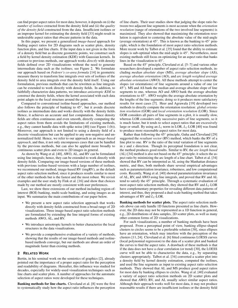
Fig. 3. (a-c) Results of isoRV with increasing m (number of isovalue sam-ples), and equivalently, with increasing number of isolines. (d) Densityfield input. (e) Result of our imgRV.
following three major steps for computing the aspect ratios (see alsothe running example shown in Figure 2):
(i) Density field construction. This step is obsolete if the input isalready given as a density field (e.g., from continuous scatter plots [1]or from an image). In the case of scatter plots, a density field isconstructed from the sample points:
Φ :~xi 7−→ ρ(~xi) , where ~xi ∈Ω⊂ R2 and ρ ∈ R . (1)
Since the solution of α is unknown at the moment, the density field issimply constructed in Ω with a default aspect ratio α = 1. The approachconstructs the density field based on the prominence of~xi in Ω usingKernel Density Estimation (KDE):
ρ(~x) =1n
n
∑i=1
K~H(~x−~xi) , for ~x ∈Ω , (2)
where K~H(~x) is a kernel function with bandwidth matrix ~H. Typicalchoices for the kernel function are Gaussian and Epanechnikov func-tions, and we use the Gaussian function here. Typically, the densityfield is sampled on a uniform grid (image) over the domain of Ω.
(ii) Isoline extraction. Once the density field (ρ) is available, theapproach finds the density value range, normalizes ρ to [0,1], uniformlysamples m isovalues (denoted as ti, i = 1, · · · ,m) in [0,1], and extractsa set of isolines (denoted as L(ti)) for each isovalue ti.
(iii) Aspect ratio computation. In the last step, the approach gathersthe line segments of the isolines, and applies an existing aspect ratioselection method (e.g., AL or RV) to determine the aspect ratio.
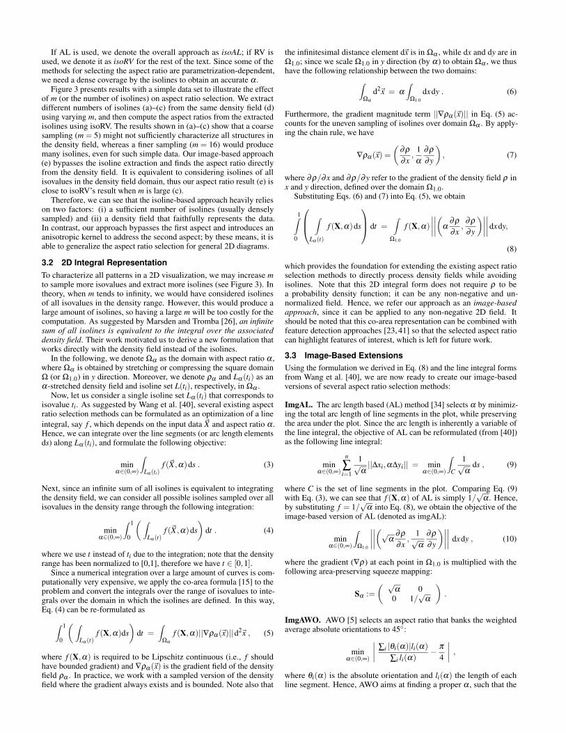
If AL is used, we denote the overall approach as isoAL; if RV isused, we denote it as isoRV for the rest of the text. Since some of themethods for selecting the aspect ratio are parametrization-dependent,we need a dense coverage by the isolines to obtain an accurate α .
Figure 3 presents results with a simple data set to illustrate the effectof m (or the number of isolines) on aspect ratio selection. We extractdifferent numbers of isolines (a)–(c) from the same density field (d)using varying m, and then compute the aspect ratios from the extractedisolines using isoRV. The results shown in (a)–(c) show that a coarsesampling (m = 5) might not sufficiently characterize all structures inthe density field, whereas a finer sampling (m = 16) would producemany isolines, even for such simple data. Our image-based approach(e) bypasses the isoline extraction and finds the aspect ratio directlyfrom the density field. It is equivalent to considering isolines of allisovalues in the density field domain, thus our aspect ratio result (e) isclose to isoRV’s result when m is large (c).
Therefore, we can see that the isoline-based approach heavily relieson two factors: (i) a sufficient number of isolines (usually denselysampled) and (ii) a density field that faithfully represents the data.In contrast, our approach bypasses the first aspect and introduces ananisotropic kernel to address the second aspect; by these means, it isable to generalize the aspect ratio selection for general 2D diagrams.
3.2 2D Integral RepresentationTo characterize all patterns in a 2D visualization, we may increase mto sample more isovalues and extract more isolines (see Figure 3). Intheory, when m tends to infinity, we would have considered isolinesof all isovalues in the density range. However, this would produce alarge amount of isolines, so having a large m will be too costly for thecomputation. As suggested by Marsden and Tromba [26], an infinitesum of all isolines is equivalent to the integral over the associateddensity field. Their work motivated us to derive a new formulation thatworks directly with the density field instead of the isolines.
In the following, we denote Ωα as the domain with aspect ratio α ,where Ωα is obtained by stretching or compressing the square domainΩ (or Ω1.0) in y direction. Moreover, we denote ρα and Lα (ti) as anα-stretched density field and isoline set L(ti), respectively, in Ωα .
Now, let us consider a single isoline set Lα (ti) that corresponds toisovalue ti. As suggested by Wang et al. [40], several existing aspectratio selection methods can be formulated as an optimization of a lineintegral, say f , which depends on the input data ~X and aspect ratio α .Hence, we can integrate over the line segments (or arc length elementsds) along Lα (ti), and formulate the following objective:
minα∈(0,∞)
∫Lα (ti)
f (~X ,α)ds . (3)
Next, since an infinite sum of all isolines is equivalent to integratingthe density field, we can consider all possible isolines sampled over allisovalues in the density range through the following integration:
minα∈(0,∞)
∫ 1
0
( ∫Lα (t)
f (~X ,α)ds)
dt . (4)
where we use t instead of ti due to the integration; note that the densityrange has been normalized to [0,1], therefore we have t ∈ [0,1].
Since a numerical integration over a large amount of curves is com-putationally very expensive, we apply the co-area formula [15] to theproblem and convert the integrals over the range of isovalues to inte-grals over the domain in which the isolines are defined. In this way,Eq. (4) can be re-formulated as∫ 1
0
( ∫Lα (t)
f (X,α)ds)
dt =∫
Ωα
f (X,α)||∇ρα (~x)||d2~x , (5)
where f (X,α) is required to be Lipschitz continuous (i.e., f shouldhave bounded gradient) and ∇ρα (~x) is the gradient field of the densityfield ρα . In practice, we work with a sampled version of the densityfield where the gradient always exists and is bounded. Note also that
the infinitesimal distance element d~x is in Ωα , while dx and dy are inΩ1.0; since we scale Ω1.0 in y direction (by α) to obtain Ωα , we thushave the following relationship between the two domains:∫
Ωα
d2~x = α
∫Ω1.0
dxdy . (6)
Furthermore, the gradient magnitude term ||∇ρα (~x)|| in Eq. (5) ac-counts for the uneven sampling of isolines over domain Ωα . By apply-ing the chain rule, we have
∇ρα (~x) =(
∂ρ
∂x,
1α
∂ρ
∂y
), (7)
where ∂ρ/∂x and ∂ρ/∂y refer to the gradient of the density field ρ inx and y direction, defined over the domain Ω1.0.
Substituting Eqs. (6) and (7) into Eq. (5), we obtain
1∫0
∫Lα (t)
f (X,α)ds
dt =∫
Ω1.0
f (X,α)
∣∣∣∣∣∣∣∣(α∂ρ
∂x,
∂ρ
∂y
)∣∣∣∣∣∣∣∣dxdy,
(8)
which provides the foundation for extending the existing aspect ratioselection methods to directly process density fields while avoidingisolines. Note that this 2D integral form does not require ρ to bea probability density function; it can be any non-negative and un-normalized field. Hence, we refer our approach as an image-basedapproach, since it can be applied to any non-negative 2D field. Itshould be noted that this co-area representation can be combined withfeature detection approaches [23, 41] so that the selected aspect ratiocan highlight features of interest, which is left for future work.
3.3 Image-Based ExtensionsUsing the formulation we derived in Eq. (8) and the line integral formsfrom Wang et al. [40], we are now ready to create our image-basedversions of several aspect ratio selection methods:
ImgAL. The arc length based (AL) method [34] selects α by minimiz-ing the total arc length of line segments in the plot, while preservingthe area under the plot. Since the arc length is inherently a variable ofthe line integral, the objective of AL can be reformulated (from [40])as the following line integral:
minα∈(0,∞)
n
∑i=1
1√α||∆xi,α∆yi|| = min
α∈(0,∞)
∫C
1√α
ds , (9)
where C is the set of line segments in the plot. Comparing Eq. (9)with Eq. (3), we can see that f (X,α) of AL is simply 1/
√α . Hence,
by substituting f = 1/√
α into Eq. (8), we obtain the objective of theimage-based version of AL (denoted as imgAL):
minα∈(0,∞)
∫Ω1.0
∣∣∣∣∣∣∣∣(√α∂ρ
∂x,
1√α
∂ρ
∂y
)∣∣∣∣∣∣∣∣ dxdy , (10)
where the gradient (∇ρ) at each point in Ω1.0 is multiplied with thefollowing area-preserving squeeze mapping:
Sα :=( √
α 00 1/
√α
).
ImgAWO. AWO [5] selects an aspect ratio that banks the weightedaverage absolute orientations to 45:
minα∈(0,∞)
∣∣∣∣ ∑i |θi(α)|li(α)
∑i li(α)− π
4
∣∣∣∣ ,where θi(α) is the absolute orientation and li(α) the length of eachline segment. Hence, AWO aims at finding a proper α , such that the
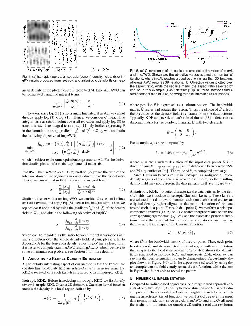
Fig. 4. (a) Isotropic (top) vs. anisotropic (bottom) density fields. (b, c) Im-gRV results produced from isotropic and anisotropic density fields, resp.
mean density of the plotted curve is close to π/4. Like AL, AWO canbe formulated using line integral terms:
minα∈(0,∞)
∣∣∣∣ ∫C |θ(α)|ds∫C ds
− π
4
∣∣∣∣ . (11)
However, since Eq. (11) is not a single line integral as AL, we cannotdirectly apply Eq. (8) to Eq. (11). Hence, we consider C in each lineintegral term as sets of isolines over all isovalues and apply Eq. (8) totransform each line integral term in Eq. (11). By further expressing θ
in the formulation using gradients ∂ρ
∂x and ∂ρ
∂y in Ω1.0, we can obtainthe following objective of imgAWO:
minα∈(0,∞)
∣∣∣∣∣∣∫
Ω1.0
∣∣∣tan−1(
α∂ρ
∂x /∂ρ
∂y
)∣∣∣ ∣∣∣∣∣∣(α∂ρ
∂x ,∂ρ
∂y
)∣∣∣∣∣∣dxdy∫Ω1.0
∣∣∣∣∣∣(α∂ρ
∂x ,∂ρ
∂y
)∣∣∣∣∣∣dxdy− π
4
∣∣∣∣∣∣ , (12)
which is subject to the same optimization process as AL. For the deriva-tion details, please refer to the supplemental materials.
ImgRV. The resultant vector (RV) method [29] takes the ratio of thetotal variation of line segments in x and y direction as the aspect ratio.Hence, we can write it in the following line integral form:
α =∑i |∆xi|∑i |∆yi|
=
∫C |cosθ |ds∫C |sinθ |ds
. (13)
Similar to the derivation for imgAWO, we consider C as sets of isolinesover all isovalues and apply Eq. (8) to each line integral term. Then, wereplace cosθ and sinθ by using the gradients ∂ρ
∂x and ∂ρ
∂y of the densityfield in Ω1.0 and obtain the following objective of imgRV:
α =
∫Ω1.0|| ∂ρ
∂y ||dxdy∫Ω1.0|| ∂ρ
∂x ||dxdy, (14)
which can be regarded as the ratio between the total variations in xand y direction over the whole density field. Again, please refer toAppendix A for the derivation details. Since imgRV has a closed form,it is faster to compute than imgAWO and imgAL, for which we have tosolve a minimization problem; see Section 5 for more details.
4 ANISOTROPIC KERNEL DENSITY ESTIMATION
A particularly interesting aspect of our method is that the kernels forconstructing the density field are selected in relation to the data. TheKDE associated with such kernels is referred to as anisotropic KDE.
Isotropic KDE. Before introducing anisotropic KDE, we first brieflyreview isotropic KDE. Given a 2D domain, a Gaussian kernel functionmodels the density in a local region defined by
K(~x) =1
2π
√|~H|
exp(−1
2~xT ~H−1~x
), (15)
Fig. 5. (a) Convergence of the conjugate gradient optimization of ImgALand ImgAWO. Shown are the objective values against the number ofiterations, where imgAL reaches a good solution in less than 30 iterations,whereas AWO requires 39 iterations. (b) Objective values plotted overthe aspect ratio, while the red line marks the aspect ratio selected byimgRV. In this example (CMC dataset [10]), all three methods find asimilar aspect ratio of 0.48, showing three clusters in circular shapes.
where position ~x is expressed as a column vector. The bandwidthmatrix ~H scales and rotates the region. Thus, the choice of ~H affectsthe precision of the density field in characterizing the data patterns.Typically, KDE adopts Silverman’s rule of thumb [33] to determine adiagonal matrix for the bandwidth matrix ~H with two elements
~H =
(hx 00 hy
).
For example, hx can be computed by
hx = 1.06×minsx,R
1.34n−1/5 , (16)
where sx is the standard deviation of the input data points X in xdirection and R = x[0.75n]− x[0.25n] is the difference between the 25%and 75% quantiles of xi. The value of hy is computed similarly.
Such Gaussian kernels result in isotropic, axis-aligned ellipticaldensity regions of the same size around each point, so the resultingdensity field may not represent the data patterns well (see Figure 4 (a)).
Anisotropic KDE. To better characterize the data patterns by the den-sity fields, we introduce anisotropic Gaussian kernels. These kernelsare selected in a data-aware manner, such that each kernel creates anelliptical density region aligned to the main orientation of the dataaround each data point. For each data point~xi, we perform a principalcomponent analysis (PCA) on its k nearest neighbors and obtain thecorresponding eigenvectors ν1
i ,ν2i and the associated principal direc-
tions. Since the principal directions maximize data variance, we usethem to adjust the shape of the Gaussian function:
~Hi = ~H [ν1i ;ν
2i ] , (17)
where ~Hi is the bandwidth matrix of the i-th point. Thus, each pointhas its own ~Hi and its associated elliptical region with an orientationthat adapts to the local data pattern. Figure 4(a) shows the densityfields generated by isotropic KDE and anisotropic KDE, where we cansee that the local orientation is clearly characterized. Accordingly, theplot shown in Figure 4(d) with the aspect ratio selected by using theanisotropic density field clearly reveal the sin function, while the onein Figure 4(c) is not able to reveal the pattern.
5 NUMERICAL IMPLEMENTATION
Compared to isoline-based approaches, our image-based approach con-sists of only two steps: (i) density field construction and (ii) aspect ratiocomputation. To accelerate the k nearest neighbor search for construct-ing the anisotropic kernel function, we build a k-d tree over the inputdata points. In addition, since imgAL, imgAWO, and imgRV all needthe gradient information, we sample a 2D uniform grid at a resolution
of wg× hg over the density field ρ and perform the Sobel operatorto compute the gradient field ∇ρ , where wg and hg are empiricallyset as 1000. Doing so, we are able to accelerate the computation ofthe integrals in Eqs. (10), (12), and (14), which are implemented as aRiemann sum over all grid points in the domain.
To calculate the optimal aspect ratio for imgAL and imgAWO, wenumerically find the value that minimizes the objective functions fromEqs. (10) and (12) by using the conjugate gradient method [17]. LikeTalbot et al. [34], we parametrize the 1D search problem with log(α),this lets the optimization converge in less than 30 iterations. Theoptimal aspect ratio for imgRV can also be easily obtained by directlyusing Eq. (14). Figure 5 presents an exemplary result in which all threemethods find very similar optimal aspect ratios; a more comprehensiveevaluation will be presented in Section 6.1.
We implemented our approach in R (see code in supplemental ma-terials) and ran it on a machine with an Intel® Core™ i5-4200H with2.8 GHz dual-core CPU in double precision. Our experiments on 100datasets showed that imgRV mostly took around 50 to 300 ms, thusallowing for interactive manipulation; see Section 6.1 for details. Theperformance could be further boosted up by exploiting parallel compu-tation on the GPU.
6 EVALUATION
We performed four experiments to evaluate our image-based methods.First, we quantitatively compared our methods with isoline-based meth-ods (Section 6.1) for two purposes: (i) learn to see if our methodsproduce similar aspect ratios as isoline-based methods but in less time,and (ii) find out, which one of our three methods is fastest and most ro-bust. Second, we studied the convergence of our image-based methodswith isoline-based methods and the corresponding methods designedfor line charts (Section 6.2). Next, we presented a parameter analysisto find proper parameters for the best method recommended by the firstexperiment (Section 6.3). Lastly, we configured the best method withproper parameters, and revisited the user study by Fink et al. [16] toshow that choices made by our method are mostly consistent with theuser preferences (Section 6.4).
6.1 Quantitative Comparison with Isoline-based MethodsComparing extensively with various methods, Wang et al. [40] showedthat the RV method not only produces similar results to classical meth-ods such as AWO and AL, but also is the fastest and most robust. Onthe other side, Talbot et al. [34] extended various aspect ratio selectionmethods designed for line charts (including RV) into isoline-basedmethods to work for scatter plots. Therefore, we selected the isoline-based RV method (isoRV) as a representative of isoline-based methods,but extracted a large number of isolines for isoRV to capture most ofthe structures in the data. To be specific, we computed a 1000×1000density field for each dataset. In addition, we took out the effect ofanisotropic KDE, and used isotropic KDE for both isoRV and ourimage-based methods. We only summarize the comparison results withisoRV in the following, detailed comparison results with most methodsare presented in the supplementary material.
Datasets. For a comprehensive comparison, we gathered 100 scatterplots with substantial variations in terms of the number of data points,ranging from 200 to 5000. Among them, 71 datasets show the dimen-sionality reduction results provided by Sedlmair et al. [32] and the restare real bivariate datasets collected from the UCI repository [10].
Measure. To find out if our methods produce similar aspect ratios asisoRV, we measured the relative deviation of the aspect ratios selectedby our methods from the ones selected by isoRV:
deviation =αimgX −αisoRV
αisoRV∗100% , (18)
where αimgX refers to α selected by imgRV, imgAL, or imgAWO.
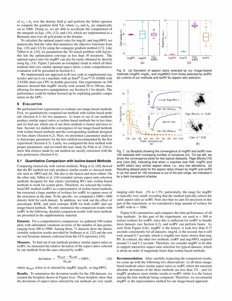
Results. To summarize the deviation results for the 100 datasets, wecreated the boxplots shown in Figure 6 (a). These boxplots show thatthe deviations of aspect ratios selected by our methods are very small,
Fig. 6. (a) Deviation of aspect ratios selected by our image-basedmethods (imgRV, imgAL, and imgAWO) from those selected by isoRV;(b) runtime of our methods and isoRV for aspect ratio selection.
Fig. 7. (a) Boxplots showing the convergence of imgRV and isoRV over100 datesets with increasing number of isovalues (m). On top left, weshow the convergence plots for two typical datasets, Page Blocks [10]and Cars [36], indicating that when m reaches over 500, imgRV andisoRV select very similar aspect ratios, i.e., very low deviations. (b)Resulting dataset plots for the aspect ratios chosen by imgRV and isoRV.In (a) the result for 100 isovalues is out of the plot range, we indicated itby a dark transparent shadow.
ranging only from −2% to 1.5%; particularly, the range for imgRVis typically very small, revealing that the method typically selects thesame aspect ratio as isoRV. Note also that we aim for precision in thispart of the experiment, so we considered a large amount of isolines forisoRV with m = 1000.
Figure 6 (b) summarizes and compares the time performance of allfour methods. In this part of the experiment, we used m = 500 toextract isolines for isoRV, since this is sufficient for isoRV to handlemost datasets (see Section 6.2), and isoRV can perform faster. Asseen from Figure 6 (b), imgRV is the fastest, it took less than 0.37seconds consistently for all datasets; imgAL is the second, but it stilltook around 0.7 seconds, which is roughly two times slower than img-RV. In contrast, the other two methods, isoRV and imgAWO, requiredaround 3.2 and 5.2 seconds. Therefore, we consider imgRV to be ableto support interactive aspect ratio selection for typical datasets, whichis about an order of magnitude faster than isoline-based methods.
Recommendation. After carefully inspecting the comparison results,we come up with the following two observations: (i) all three image-based methods select similar aspect ratios as isoRV, where the maximalabsolute deviations of the three methods are less than 2% ; and (ii)imgRV produces most similar results to isoRV, while it is the fastestamong the four methods being compared. Therefore, we recommendimgRV as the representative method for our image-based approach.
Fig. 8. Illustrating the relationship between RV and imgRV using twotime-series datasets: CO2 [6] (top) and Computer [9] (bottom). (a,d) Linecharts and aspect ratios selected by directly applying RV to the curves;(b,e) Smoothed line charts and aspect ratios selected by applying RV tothe smoothed curves shown in red; (c,f) Line charts and aspect ratiosselected by directly applying imgRV to the curves.
Fig. 9. (a) Deviation (in %) and computing time (b) for creating aspectratios for 100 datasets in domains of various resolutions: 100× 100,200×200, 500×500, and 1000×1000.
6.2 Convergence StudyWe refer the isoline-based methods and the original methods designedfor line charts as geometric methods, since both work with line seg-ments. In the second experiment, we compare their convergence withour image-based methods. Since the previous experiment showed thatimgRV produces almost the same results as isoRV, we take imgRVas the representative of image-based methods. Furthermore, we takeisoRV as the representative of isoline-based methods, and RV as therepresentative of the original methods designed for line charts.
imgRV vs. isoRV. Unlike our imgRV, the quality of aspect ratioselected by isoRV strongly depends on the amount of isolines. Hence,we tried different m over the 100 datasets in the previous experimentwhen using isoRV to select aspect ratios, and computed the deviationsin aspect ratios using Eq. (18). Figure 7 (a) summarizes the results.From the boxplots, we can see that when isoRV has a sufficiently largeamount of isolines (i.e., large m) as inputs, the aspect ratios selectedby imgRV and isoRV converge. However, isoRV typically requires atleast m=500 for most datasets. Thanks to the image-based formulation,our approach (imgRV) can bypass the isoline construction and directlycompute the aspect ratios from the density fields.
imgRV vs. RV. By converting line charts to density fields, our methodscan also be used to find aspect ratios for line charts. Since density fieldsare smooth representations of the original line charts, our imgRV maynot produce similar aspect ratios as RV, which works on the unsmoothedpolygonal data. Hence, if we properly smooth the data, imgRV andRV might produce similar aspect ratios. Figures 8 (a, b, c) show resultsproduced with RV, smoothed RV, and imgRV using the CO2 dataset [6],where a similar upward trend is clearly observable in Figures 8 (b, c).
Fig. 10. Influence of the number of nearest neighbors (k) on the con-structed anisotropic density field and the aspect ratios selected byimgRV on the eFashion dataset [13]. (a) Density field constructed byisotropic KDE and its resulting plot; (b, c, d) Density fields constructed byanisotropic KDE with different k and the resulting plots.
Figures 8 (d, e, f) show the Computer dataset [9], which further confirmsour observation that applying RV to smoothed data produces aspectratios similar to the ones selected by imgRV.
6.3 Parameter AnalysisIn the third experiment, we studied how to select the resolution ofdensity fields and number of nearest neighbors for our image-basedmethods (typically, imgRV):
(i) Resolution of density fields. Patterns in data are generally bettercharacterized by density fields of higher resolution, but this increasesthe required computing time. Hence, we performed an experiment tofind the proper resolution for revealing all necessary aspects of the datawhile consuming less computing time. We considered four differentresolutions: 100×100, 200×200, 500×500, and 1000×1000, and ap-plied imgRV to compute the aspect ratio for each of the 100 datasetsdescribed in Section 6.1. To study the influence of the resolution, weagain used the deviation measure defined in Section 6.1 and took theaspect ratios computed with the highest resolution as the references.
Figure 9 (a) summarizes the results for the 100 datasets. It showsthat the deviations for a resolution of 500×500 are in a small range of[−0.2%,0.15%], thus the aspect ratios selected with domain resolutions500×500 are similar to those selected with 1000×1000. Figure 9 (b)summarizes the time performance of imgRV for different resolutions;it shows that the computational time increases non-linearly with thedomain resolution. Considering these two results, we recommend500×500 as the default resolution for our density fields.
(ii) Number of nearest neighbors (k). Next, we attempted to empiri-cally find a proper value of k for constructing the anisotropic densityfields; see Figures 4 and 10 for results on two typical datasets. Fromthe analysis, we found that similar k tends to produce similar aspectratios, but if k is too large, it might lead to obscuration of interestingpatterns; see Figure 10 (d). Therefore, we set the default k as five anduse this value to produce all the results shown in the paper.
Initially, we attempted to perform an analysis with the deviation mea-sure to explore imgRV and isoRV for different k, similar to the previousexperiments. However, k affects the density fields and so are imgRVand isoRV, so both methods produce similar aspect ratios for varyingk. However, since imgRV allows interactive exploration, users mayadjust k to explore the plot like multi-scale banking. Indeed, k is data-dependent; in the future, we plan to investigate ways to automaticallydecide proper values of k in terms of the data characteristics.
6.4 Revisiting the Study of Fink’s MethodIn the last experiment, we revisited the study in [16] to show that ourmethod yields results that are quite close to the ones produced by thebest two criteria in [16], but also consistent with the user preferences.Fink et al. [16] studied various geometric criteria to select aspect ratios,and found that the criteria of minimizing the total length and minimiz-ing the mean uncompactness yielded the best results, so we compared
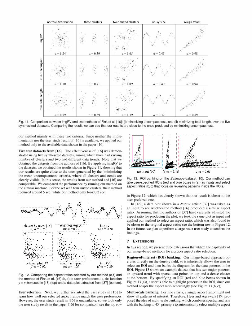
Fig. 11. Comparison between imgRV and two methods of Fink et al. [16]: (i) minimizing uncompactness, and (ii) minimizing total length, over the fivesynthesized datasets. Comparing the result, we can see that our results are close to the ones produced by minimizing uncompactness.
our method mainly with these two criteria. Since neither the imple-mentation nor the user study result of [16] is available, we applied ourmethod only to the available data shown in the paper [16].
Five test datasets from [16]. The effectiveness of [16] was demon-strated using five synthesized datasets, among which three had varyingnumber of clusters and two had different data trends. Note that weobtained the datasets from the authors of [16]. By applying imgRV tothe datasets, we obtained the results shown in Figure 11, showing thatour results are quite close to the ones generated by the “minimizingthe mean uncompactness” criteria, where all clusters and trends areclearly visible. In this sense, the results from our method and [16] arecomparable. We compared the performance by running our method onthe similar machine. For the set with four mixed clusters, their methodrequired around 5 sec. while our method only took 0.2 sec.
Fig. 12. Comparing the aspect ratios selected by our method (c, f) andthe method of Fink et al. [16] (b, e) to user preferences (a, d): functiony = xsinx used in [16] (top) and a data plot extracted from [37] (bottom).
User selection. Next, we further revisited the user study in [16] tolearn how well our selected aspect ratios match the user preferences.However, the user study result in [16] is unavailable, so we took onlythe user study result in the paper [16] for comparison; see the top row
Fig. 13. ROI banking on the Satimage dataset [10]. Our method cantake user-specified ROIs (red and blue boxes in (a)) as inputs and selectaspect ratios (b, c) that focus on revealing patterns inside the ROIs.
in Figure 12, which has clearly shown that our result is closer to theuser preferred one.
In [16], a data plot shown in a Nature article [37] was taken asan input to see whether the method [16] produced a similar aspectratio. Assuming that the authors of [37] have carefully adjusted theaspect ratio for producing the plot, we took the same plot as input andapplied our method to select an aspect ratio, which was also found tobe closer to the original aspect ratio; see the bottom row in Figure 12.In the future, we plan to perform a large-scale user study to confirm thefindings.
7 EXTENSIONS
In this section, we present three extensions that utilize the capability ofour image-based methods for a proper aspect ratio selection.
Region-of-interest (ROI) banking. Our image-based approach op-erates directly on the density field, so it inherently allows the user toselect an ROI and then banks the diagram for the data patterns in theROI. Figure 13 shows an example dataset that has two major patterns:an upward trend with sparse data points on top and a dense clusterat the bottom. By specifying an ROI (red and blue boxes shown inFigure 13 (a)), a user is able to highlight patterns in the ROI, since ourmethod adapts the aspect ratio accordingly (see Figure 13 (b, c)).
Multi-scale banking. For line charts, a single aspect ratio might notshow all patterns of interest. Therefore, Heer and Agrawala [19] pro-posed the idea of multi-scale banking, which combines spectral analysiswith the banking to 45 principle to automatically select multiple aspect
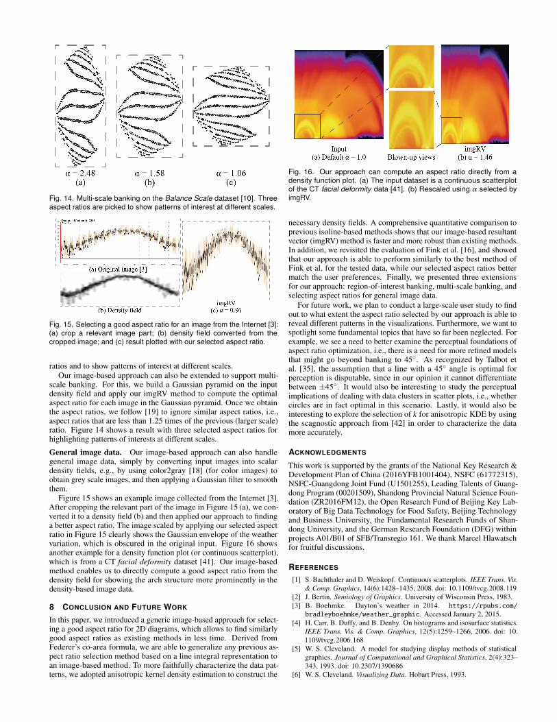
Fig. 14. Multi-scale banking on the Balance Scale dataset [10]. Threeaspect ratios are picked to show patterns of interest at different scales.
Fig. 15. Selecting a good aspect ratio for an image from the Internet [3]:(a) crop a relevant image part; (b) density field converted from thecropped image; and (c) result plotted with our selected aspect ratio.
ratios and to show patterns of interest at different scales.Our image-based approach can also be extended to support multi-
scale banking. For this, we build a Gaussian pyramid on the inputdensity field and apply our imgRV method to compute the optimalaspect ratio for each image in the Gaussian pyramid. Once we obtainthe aspect ratios, we follow [19] to ignore similar aspect ratios, i.e.,aspect ratios that are less than 1.25 times of the previous (larger scale)ratio. Figure 14 shows a result with three selected aspect ratios forhighlighting patterns of interests at different scales.
General image data. Our image-based approach can also handlegeneral image data, simply by converting input images into scalardensity fields, e.g., by using color2gray [18] (for color images) toobtain grey scale images, and then applying a Gaussian filter to smooththem.
Figure 15 shows an example image collected from the Internet [3].After cropping the relevant part of the image in Figure 15 (a), we con-verted it to a density field (b) and then applied our approach to findinga better aspect ratio. The image scaled by applying our selected aspectratio in Figure 15 clearly shows the Gaussian envelope of the weathervariation, which is obscured in the original input. Figure 16 showsanother example for a density function plot (or continuous scatterplot),which is from a CT facial deformity dataset [41]. Our image-basedmethod enables us to directly compute a good aspect ratio from thedensity field for showing the arch structure more prominently in thedensity-based image data.
8 CONCLUSION AND FUTURE WORK
In this paper, we introduced a generic image-based approach for select-ing a good aspect ratio for 2D diagrams, which allows to find similarlygood aspect ratios as existing methods in less time. Derived fromFederer’s co-area formula, we are able to generalize any previous as-pect ratio selection method based on a line integral representation toan image-based method. To more faithfully characterize the data pat-terns, we adopted anisotropic kernel density estimation to construct the
Fig. 16. Our approach can compute an aspect ratio directly from adensity function plot. (a) The input dataset is a continuous scatterplotof the CT facial deformity data [41]. (b) Rescaled using α selected byimgRV.
necessary density fields. A comprehensive quantitative comparison toprevious isoline-based methods shows that our image-based resultantvector (imgRV) method is faster and more robust than existing methods.In addition, we revisited the evaluation of Fink et al. [16], and showedthat our approach is able to perform similarly to the best method ofFink et al. for the tested data, while our selected aspect ratios bettermatch the user preferences. Finally, we presented three extensionsfor our approach: region-of-interest banking, multi-scale banking, andselecting aspect ratios for general image data.
For future work, we plan to conduct a large-scale user study to findout to what extent the aspect ratio selected by our approach is able toreveal different patterns in the visualizations. Furthermore, we want tospotlight some fundamental topics that have so far been neglected. Forexample, we see a need to better examine the perceptual foundations ofaspect ratio optimization, i.e., there is a need for more refined modelsthat might go beyond banking to 45. As recognized by Talbot etal. [35], the assumption that a line with a 45 angle is optimal forperception is disputable, since in our opinion it cannot differentiatebetween ±45. It would also be interesting to study the perceptualimplications of dealing with data clusters in scatter plots, i.e., whethercircles are in fact optimal in this scenario. Lastly, it would also beinteresting to explore the selection of k for anisotropic KDE by usingthe scagnostic approach from [42] in order to characterize the datamore accurately.
ACKNOWLEDGMENTS
This work is supported by the grants of the National Key Research &Development Plan of China (2016YFB1001404), NSFC (61772315),NSFC-Guangdong Joint Fund (U1501255), Leading Talents of Guang-dong Program (00201509), Shandong Provincial Natural Science Foun-dation (ZR2016FM12), the Open Research Fund of Beijing Key Lab-oratory of Big Data Technology for Food Safety, Beijing Technologyand Business University, the Fundamental Research Funds of Shan-dong University, and the German Research Foundation (DFG) withinprojects A01/B01 of SFB/Transregio 161. We thank Marcel Hlawatschfor fruitful discussions.
REFERENCES
[1] S. Bachthaler and D. Weiskopf. Continuous scatterplots. IEEE Trans. Vis.& Comp. Graphics, 14(6):1428–1435, 2008. doi: 10.1109/tvcg.2008.119
[2] J. Bertin. Semiology of Graphics. University of Wisconsin Press, 1983.[3] B. Boehmke. Dayton’s weather in 2014. https://rpubs.com/
bradleyboehmke/weather_graphic. Accessed January 2, 2015.[4] H. Carr, B. Duffy, and B. Denby. On histograms and isosurface statistics.
IEEE Trans. Vis. & Comp. Graphics, 12(5):1259–1266, 2006. doi: 10.1109/tvcg.2006.168
[5] W. S. Cleveland. A model for studying display methods of statisticalgraphics. Journal of Computational and Graphical Statistics, 2(4):323–343, 1993. doi: 10.2307/1390686
[6] W. S. Cleveland. Visualizing Data. Hobart Press, 1993.
[7] W. S. Cleveland. The Elements of Graphing Data. Wadsworth AdvancedBooks and Software, 1994.
[8] W. S. Cleveland, M. E. McGill, and R. McGill. The shape parameter ofa two-variable graph. Journal of the American Statistical Association,83(402):289–300, 1988. doi: 10.1080/01621459.1988.10478598
[9] Y. Croissant. Ecdat: Data Sets for Econometrics, 2016. R package version0.3-1.
[10] D. Dheeru and E. Karra Taniskidou. UCI machine learning repository,2017. http://archive.ics.uci.edu/ml.
[11] T. M. Dijkstra, B. Liu, and S. Oomes. Perception of ellipse orientation:data and Bayesian model. Journal of Vision, 3(9):11–11, 2003. doi: 10.1167/3.9.11
[12] B. Duffy, H. Carr, and T. Moller. Integrating isosurface statistics andhistograms. IEEE Trans. Vis. & Comp. Graphics, 19(2):263–277, 2013.doi: 10.1109/tvcg.2012.118
[13] F. Farber, S. K. Cha, J. Primsch, C. Bornhovd, S. Sigg, and W. Lehner. Saphana database: data management for modern business applications. ACMSIGMOD Record, 40(4):45–51, 2012. doi: 10.1145/2094114.2094126
[14] H. Federer. Curvature measures. Transactions of the American Mathemat-ical Society, 93(3):418–491, 1959. doi: 10.2307/1993504
[15] H. Federer. Geometric Measure Theory. Springer, 1996.[16] M. Fink, J.-H. Haunert, J. Spoerhase, and A. Wolff. Selecting the aspect
ratio of a scatter plot based on its Delaunay triangulation. IEEE Trans.Vis. & Comp. Graphics, 19(12):2326–2335, 2013. doi: 10.1109/tvcg.2013.187
[17] J. C. Gilbert and J. Nocedal. Global convergence properties of conjugategradient methods for optimization. SIAM Journal on Optimization, 2(1):21–42, 1992. doi: 10.1137/0802003
[18] A. A. Gooch, S. C. Olsen, J. Tumblin, and B. Gooch. Color2gray: salience-preserving color removal. ACM Trans. on Graph., 24(3):634–639, 2005.doi: 10.1145/1073204.1073241
[19] J. Heer and M. Agrawala. Multi-scale banking to 45º. IEEE Trans. Vis. &Comp. Graphics, 12(5):701–708, 2006. doi: 10.1109/tvcg.2006.163
[20] J. Heinrich and D. Weiskopf. Continuous parallel coordinates. IEEE Trans.Vis. & Comp. Graphics, 15(6):1531–1538, 2009. doi: 10.1109/tvcg.2009.131
[21] R. Hyndman. fma: Data sets from forecasting: methods and applicationsby Makridakis, Wheelwright & Hyndman (1998). R package version, 2,2009.
[22] O. D. Lampe and H. Hauser. Curve density estimates. Computer GraphicsForum, 30(3):633–642, 2011. doi: 10.1111/j.1467-8659.2011.01912.x
[23] D. J. Lehmann and H. Theisel. Discontinuities in continuous scatter plots.IEEE Trans. Vis. & Comp. Graphics, 16(6):1291–1300, 2010. doi: 10.1109/tvcg.2010.146
[24] G. Loffler. Perception of contours and shapes: Low and intermediate stagemechanisms. Vision Research, 48(20):2106–2127, 2008. doi: 10.1016/j.visres.2008.03.006
[25] J. Mackinlay. Automating the design of graphical presentations of rela-tional information. ACM Trans. on Graph., 5(2):110–141, 1986. doi: 10.1145/22949.22950
[26] J. E. Marsden and A. Tromba. Vector Calculus. Macmillan, 2003.[27] V. Molchanov, A. Fofonov, and L. Linsen. Continuous representation
of projected attribute spaces of multifields over any spatial sampling.Computer Graphics Forum, 32(3):301–310, 2013. doi: 10.1111/cgf.12117
[28] F. Morgan. Geometric Measure Theory: A Beginner’s Guide. AcademicPress, 2016.
[29] G. Saptarshi and W. S. Cleveland. Perceptual, mathematical, and statisticalproperties of judging functional dependence on visual displays. Technicalreport, Purdue University Department of Statistics, 2011.
[30] A. Sarikaya and M. Gleicher. Scatterplots: Tasks, data, and designs. IEEETrans. Vis. & Comp. Graphics, 24(1):402–412, 2018. doi: 10.1109/tvcg.2017.2744184
[31] C. E. Scheidegger, J. Schreiner, B. Duffy, H. Carr, and C. T. Silva. Re-visiting histograms and isosurface statistics. IEEE Trans. Vis. & Comp.Graphics, 14(6):1659–1666, 2008. doi: 10.1109/tvcg.2008.160
[32] M. Sedlmair, A. Tatu, T. Munzner, and M. Tory. A taxonomy of visualcluster separation factors. Computer Graphics Forum, 31(3):1335–1344,2012. doi: 10.1111/j.1467-8659.2012.03125.x
[33] B. W. Silverman. Density Estimation for Statistics and Data Analysis.CRC Press, 1986.
[34] J. Talbot, J. Gerth, and P. Hanrahan. Arc length-based aspect ratio selection.IEEE Trans. Vis. & Comp. Graphics, 17(12):2276–2282, 2011. doi: 10.1109/tvcg.2011.167
[35] J. Talbot, J. Gerth, and P. Hanrahan. An empirical model of slope ratiocomparisons. IEEE Trans. Vis. & Comp. Graphics, 18(12):2613–2620,2012. doi: 10.1109/tvcg.2012.196
[36] A. Tatu, G. Albuquerque, M. Eisemann, J. Schneidewind, H. Theisel,M. Magnork, and D. Keim. Combining automated analysis and visual-ization techniques for effective exploration of high-dimensional data. InProc. IEEE Symposium on Visual Analytics Science and Technology, pp.59–66, 2009. doi: 10.1109/vast.2009.5332628
[37] W. Volkmuth and R. Austin. DNA electrophoresis in microlithographicarrays. Nature, 358(6387):600, 1992. doi: 10.1038/358600a0
[38] J. Wagemans. Detection of visual symmetries. Spatial Vision, 9(1):9–32,1995. doi: 10.1163/156856895x00098
[39] Y. Wang, F. Han, L. Zhu, O. Deussen, and B. Chen. Line graph or scatterplot? Automatic selection of methods for visualizing trends in time series.IEEE Trans. Vis. & Comp. Graphics, 24(2):1141–1154, 2018. doi: 10.1109/tvcg.2017.2653106
[40] Y. Wang, Z. Wang, L. Zhu, J. Zhang, C.-W. Fu, Z. Cheng, C. Tu, andB. Chen. Is there a robust technique for selecting aspect ratios in linecharts? IEEE Trans. Vis. & Comp. Graphics, to appear, 2018. doi: 10.1109/tvcg.2017.2787113
[41] Y. Wang, J. Zhang, D. J. Lehmann, H. Theisel, and X. Chi. Automatingtransfer function design with valley cell-based clustering of 2D densityplots. Computer Graphics Forum, 31(3):1295–1304, 2012. doi: 10.1111/j.1467-8659.2012.03122.x
[42] L. Wilkinson, A. Anand, and R. L. Grossman. Graph-theoretic scagnostics.In Proceedings of the IEEE Symposium on Information Visualization, pp.157–164, 2005. doi: 10.1109/infvis.2005.1532142


![ZHIYUAN WANG AND JIAN ZHOU arXiv:1812.10638v1 [math.AG] … · arXiv:1812.10638v1 [math.AG] 27 Dec 2018 ORBIFOLD EULER CHARACTERISTICS OF Mg,n ZHIYUAN WANG AND JIAN ZHOU Abstract.](https://static.fdocument.org/doc/165x107/5f0cdd7d7e708231d43783df/zhiyuan-wang-and-jian-zhou-arxiv181210638v1-mathag-arxiv181210638v1-mathag.jpg)