Golden Ratio Algorithms for Variational Inequalities

Yura Malitsky∗

Abstract

The paper presents a fully explicit algorithm for monotone variational inequal-ities. The method uses variable stepsizes that are computed using two previousiterates as an approximation of the local Lipschitz constant without running a line-search. Thus, each iteration of the method requires only one evaluation of a mono-tone operator F and a proximal mapping g. The operator F need not be Lipschitz-continuous, which also makes the algorithm interesting in the area of compositeminimization where one cannot use the descent lemma. The method exhibits anergodic O(1/k) convergence rate and R-linear rate, if F, g satisfy the error boundcondition. We discuss possible applications of the method to fixed point problems.Furthermore, we show theoretically that the method still converges under a newrelaxed monotonicity condition and confirm numerically that it can robustly workeven for some highly nonmonotone/nonconvex problems.

2010 Mathematics Subject Classification: 47J20, 65K10, 65K15, 65Y20, 90C33Keywords: variational inequality, first-order methods, linesearch, saddle point problem,composite minimization, fixed point problem

1 IntroductionWe are interested in the variational inequality (VI) problem:

find z∗ ∈ E s.t. 〈F (z∗), z − z∗〉+ g(z)− g(z∗) ≥ 0 ∀z ∈ E , (1)

where E is a finite dimensional vector space and we assume that

(C1) the solution set S of (1) is nonempty;

(C2) g : E → (−∞,+∞] is a proper convex lower semicontinuous (lsc) function;

(C3) F : dom g → E is monotone: 〈F (u)− F (v), u− v〉 ≥ 0 ∀u, v ∈ dom g.

The function g can be nonsmooth, and it is very common to consider VI with g = δC , theindicator function of C, however we prefer a more general case. It is clear that one canrewrite (1) as a monotone inclusion: 0 ∈ (F + ∂g)(x∗). Henceforth, we implicitly assumethat we can (relatively simply) compute the resolvent (proximal operator) of g, that is(Id +∂g)−1, but cannot do this for F , in other words computing the resolvent (Id +F )−1

is prohibitively expensive.∗Institute for Numerical and Applied Mathematics, University of Göttingen, 37083 Göttingen, Ger-

many, E-Mail: y.malitskyi@math.uni-goettingen.de

1

arX

iv:1

803.

0883

2v1

[m

ath.

OC

] 2

3 M

ar 2

018

VI is a useful way to reduce many different problems that arise in optimization, PDE,control theory, games theory to a common problem (1). We recommend [17,25] as excellentreferences for a broader familiarity with the subject.

As a motivation from the optimization point of view, we present two sources whereVI naturally arise. The first example is a convex-concave saddle point problem:

minx

maxyL(x, y) := g1(x) +K(x, y)− g2(y), (2)

where x ∈ Rn, y ∈ Rm, g1 : Rn → (−∞,+∞], g2 : Rm → (−∞,+∞] are proper convex lscfunctions and K : dom g1×dom g2 → R is a smooth convex-concave function. By writingdown the first-order optimality condition, it is easy to see that problem (2) is equivalentto (1) with F and g defined as

z = (x, y) F (z) =[∇xK(x, y)−∇yK(x, y)

]g(z) = g1(x) + g2(y).

Saddle point problems are ubiquitous in optimization as this is a very convenient wayto represent many nonsmooth problems, and this in turn often allows to improve thecomplexity rates from O(1/

√k) to O(1/k). Even in the simplest case when K is bilinear

form, the saddle point problem is a typical example where the two simplest iterativemethods, the forward-backward method and the Arrow-Hurwicz method (see [2]), willnot work. Korpelevich in [27] and Popov in [44] resolved this issue by presenting two-stepmethods that converge for a general monotone F . In turn, these two papers gave birthto various improvements and extensions, see [11,31,32,34,39,41,52].

Another important source of VI is a simpler problem of composite minimization

minzJ(z) := f(z) + g(z), (3)

where z ∈ Rn, f : Rn → R is a convex smooth function and g satisfies (C2). This problemis also equivalent to (1) with F = ∇f . On the one hand, it might not be so cleverto apply generic VI methods to a specific problem such as (3). Overall, optimizationmethods have better theoretical convergence rates, and this is natural, since they exploitthe fact that F is a potential operator. However, this is only true under the assumptionthat ∇f is L-Lipschitz continuous. Without such a condition, theoretical rates for the(accelerated) proximal gradient methods do not hold anymore. Recently, there has beena renewed interest in optimization methods for the case with non-Lipschitz ∇f , we referto [4, 29, 50]. An interesting idea was developed in [4], where the descent lemma wasextended to the more general case with Bregman distance. This allows one to obtaina simple method with a fixed stepsize even when ∇f is not Lipschitz. However, suchresults are not generic as they depend drastically on problem instances where one can usean appropriate Bregman distance.

For a general VI, even when F is Lipschitz-continuous but nonlinear, computing itsLipschitz constant is not an easy task. Moreover, the curvature of F can be quite different,so the stepsizes governed by the global Lipschitz constant will be very conservative. Thus,most practical methods for VI are doomed to use linesearch — an auxiliary iterativeprocedure which runs in each iteration of the algorithm until some criterion is satisfied,and it seems this is the only option for the case when F is not Lipschitz. To this end, mostknown methods for VI with a fixed stepsize have their analogues with linesearch. This isstill an active area of research rich in diverse ideas, see [8, 22, 24, 26, 33, 47, 48, 52]. Thelinesearch can be quite costly in general as it requires computing additional values of F

2

or proxg, or even both in every linesearch iteration. Moreover, the complexity estimatesbecome not so informative, as they only say how many outer iterations one needs to reachthe desired accuracy in which the number of linesearch iterations is of course not included.

Contributions. In this paper, our aim is to propose an explicit algorithm for solvingproblem (1) with F locally Lipschitz continuous. By explicit we mean that the methoddoes not require a linesearch to be run, and its stepsizes are computed explicitly usingcurrent information about the iterates. These stepsizes approximate an inverse localLipschitz constant of F , thus they are separated from zero. Each iteration of the methodneeds only one evaluation of the proximal operator and one value of F . To our knowledge,it is the first explicit method with these properties. The method is easy to implement andit satisfies all standard rates for monotone VI: ergodic O(1/k) and R-linear if the errorbound condition holds.

Our approach is to start from the simple case when F is L-Lipschitz continuous. Forthis case, we present the Golden Ratio Algorithm with a fixed stepsize, which is interestingon his own right and gives us an intuition for the more difficult case with dynamic steps.Section 2 collects these results. In section 3 we show how one can derive new algorithms forfixed point problems based on the proposed framework. In particular, instead of workingwith the standard class of nonexpansive operators, we consider a more general class ofdemi-contractive operators. Section 4 collects two extensions of the explicit Golden RatioAlgorithm. The first proposes an extension of our explicit algorithm enhanced by twoauxiliary metrics. Although it is simple theoretically, it is nevertheless still very importantin applications, where it is preferable to use different weights for different coordinates.The second extension works for the case when instead of the monotonicity assumption(C3), F satisfies 〈F (z), z〉 ≥ 0 for all z ∈ E . In section 5 we illustrate the performance ofthe method for several problems including the aforementioned nonmonotone case. Finally,section 6 concludes the paper by presenting several directions for further research.

Preliminaries. Let E be a finite-dimensional vector space equipped with inner prod-uct 〈·, ·〉 and norm ‖ · ‖ =

√〈·, ·〉. For a lsc function g : E → (−∞,+∞] by dom g

we denote the domain of g, i.e., the set {x : g(x) < +∞}. Given a closed convex setC, PC stands for the metric projection onto C, δC denotes the indicator function of Cand dist(x,C) the distance from x to C, that is dist(x,C) = ‖PCx − x‖. The prox-imal operator proxg for a proper lsc convex function g : E → (−∞,+∞] is defined asproxg(z) = argminx{g(x) + 1

2‖x − z‖2}. The following characteristic property (prox-inequality) will be frequently used:

x̄ = proxg z ⇔ 〈x̄− z, x− x̄〉 ≥ g(x̄)− g(x) ∀x ∈ E . (4)

A simple identity important in our analysis is

‖αa+ (1− α)b‖2 = α‖a‖2 + (1− α)‖b‖2 − α(1− α)‖a− b‖2 ∀a, b ∈ E ∀α ∈ R. (5)

The following important lemma will simplify the proofs of the main theorems.

Lemma 1 (Theorem 5.5 in [6]). Let (zk) ⊂ E and C ⊆ E . Suppose that (zk) is Fejérmonotone w.r.t. C, that is ‖zk+1− z‖ ≤ ‖zk − z‖ for all z ∈ C and that all cluster pointsof (zk) belong to C. Then (zk) converges to a point in C.

3

2 Golden Ratio AlgorithmsLet ϕ =

√5+12 be the golden ratio, that is ϕ2 = 1 + ϕ. The proposed Golden RAtio

ALgorithm (GRAAL for short) reads as a simple recursion:

z̄k = (ϕ− 1)zk + z̄k−1

ϕ

zk+1 = proxλg(z̄k − λF (zk)).(6)

Theorem 1. Suppose that F is L–Lipshitz-continuous and conditions (C1)–(C3) aresatisfied. Let z1, z̄0 ∈ E be arbitrary and λ ∈ (0, ϕ2L ]. Then (zk), (z̄k), generated by (6),converge to a solution of (1).Proof. By the prox-inequality (4) we have

〈zk+1 − z̄k + λF (zk), z − zk+1〉 ≥ λ(g(zk+1)− g(z)) ∀z ∈ E (7)

and〈zk − z̄k−1 + λF (zk−1), zk+1 − zk〉 ≥ λ(g(zk)− g(zk+1)). (8)

Note that zk − z̄k−1 = 1+ϕϕ

(zk − z̄k) = ϕ(zk − z̄k). Hence, we can rewrite (8) as

〈ϕ(zk − z̄k) + λF (zk−1), zk+1 − zk〉 ≥ λ(g(zk)− g(zk+1)). (9)

Summing up equations (7) and (9), and applying the cosine rule to the inner products,we obtain

‖zk+1 − z‖2 ≤ ‖z̄k − z‖2 − ‖zk+1 − z̄k‖2 + ϕ(‖zk+1 − z̄k‖2 − ‖zk+1 − zk‖2 − ‖zk − z̄k‖2)+ 2λ〈F (zk)− F (zk−1), zk − zk+1〉− 2λ

(〈F (zk), zk − z〉+ g(zk)− g(z)

). (10)

Choose z = z∗ ∈ S. By (C3), the rightmost term in (10) is nonnegative:

〈F (zk), zk − z∗〉+ g(zk)− g(z∗) ≥ 〈F (z∗), zk − z∗〉+ g(zk)− g(z∗) ≥ 0. (11)

By (5) we have

‖zk+1 − z∗‖2 = (1 + ϕ)‖z̄k+1 − z∗‖2 − ϕ‖z̄k − z∗‖2 + ϕ(1 + ϕ)‖z̄k+1 − z̄k‖2

= (1 + ϕ)‖z̄k+1 − z∗‖2 − ϕ‖z̄k − z∗‖2 + 1ϕ‖zk+1 − z̄k‖2. (12)

Combining (10) and (11) with (12), we deduce

(1 + ϕ)‖z̄k+1 − z∗‖2 ≤ (1 + ϕ)‖z̄k − z∗‖2 − ϕ(‖zk+1 − zk‖2 + ‖zk − z̄k‖2)+ 2λ‖F (zk)− F (zk−1)‖‖zk − zk+1‖. (13)

From λ ≤ ϕ2L it follows that

2λ‖F (zk)− F (zk−1)‖‖zk+1 − zk‖ ≤ ϕ

2 (‖zk − zk−1‖2 + ‖zk+1 − zk‖2),

which finally leads to

(1+ϕ)‖z̄k+1−z∗‖2+ϕ

2 ‖zk+1−zk‖2 ≤ (1+ϕ)‖z̄k−z∗‖2+ϕ

2 ‖zk−zk−1‖2−ϕ‖zk−z̄k‖2. (14)

From (14) we conclude that (z̄k) is bounded and limk→∞ ‖zk − z̄k‖ = 0. Hence, (zk) hasat least one cluster point. Taking the limit in (7) (going to the subsequences if needed)and using that ‖zk+1 − z̄k‖ → 0 and (C2), we prove that all its cluster points belong toS. An application of Lemma 1 then completes the proof.

4

Notice that the constant ϕ is chosen not arbitrary, but as the largest constant cthat satisfies 1

c≥ c − 1 in order to get rid of the term ‖zk+1 − z̄k‖2 in (10). It is

interesting to compare the proposed GRAAL with the reflected projected (proximal)gradient method [32]. At a first glance, they are quite similar: both need one F and oneproxg per iteration. The advantage of the former, however, is that F is computed at zk,which is always feasible zk ∈ dom g, due to the properties of the proximal operator. In thereflected projected (proximal) gradient method F is computed at 2zk− zk−1 which mightbe infeasible. Sometimes, as it will be illustrated in section 5, this can be important.

2.1 Explicit Golden Ratio AlgorithmIn this section we introduce our fully explicit algorithm. By this, we mean that the algo-rithm does not require knowledge of the Lipschitz constant L nor a linesearch procedure.Furthermore, for our purposes, the locally Lipschitz-continuity of F is sufficient. Thealgorithm, which we call the Explicit Golden Ratio Algorithm (EGRAAL), is presentedbelow. For simplicity, we adopt the convention 0

0 = +∞.

Algorithm 1 Explicit Golden Ratio AlgorithmInput: Choose z0, z1 ∈ E , λ0 > 0, φ ∈ (1, ϕ], λ̄ > 0. Set z̄0 = z1, θ0 = 1, ρ = 1

φ+ 1

φ2 .For k ≥ 1 do1. Find the stepsize:

λk = min{ρλk−1,

φθk−1

4λk−1

‖zk − zk−1‖2

‖F (zk)− F (zk−1)‖2 , λ̄}

(15)

2. Compute the next iterates:

z̄k = (φ− 1)zk + z̄k−1

φ(16)

zk+1 = proxλkg(z̄k − λkF (zk)). (17)

3. Update: θk = λkλk−1

φ.

Notice that in the k-th iteration we need only to compute F (zk) once and reuse thealready computed value F (zk−1). The constant λ̄ in (15) is given only to ensure that (λk)is bounded. Hence, it makes sense to choose λ̄ quite large. Although λ0 can be arbitraryfrom the theoretical point of view, from (15) it is clear that λ0 will influence further steps,so in practice we do not want to take it too small or too large. The simplest way is tochoose z0 as a small perturbation of z1 and take λ0 = ‖z1−z0‖

‖F (z1)−F (z0)‖ . This gives us anapproximation1 of the local inverse Lipschitz constant of F at z1.

Condition (15) leads to two key estimations. First, one has λk ≤ λk−1( 1φ

+ 1φ2 ), which

in turn implies θk − 1− 1φ≤ 0. Second, from φθk−1

λk−1= θkθk−1

λkone can derive

λ2k‖F (zk)− F (zk−1)‖2 ≤ θkθk−1

4 ‖zk − zk−1‖2. (18)1We assume that F (z1) 6= F (z0), otherwise choose another z0.

5

Lemma 2. If the sequence (zk) generated by Algorithm 1 is bounded then both (λk) and(θk) are bounded and separated from 0.

Proof. It is obvious that (λk) is bounded. Let us prove by induction that it is separatedfrom 0. As (zk) is bounded there exists some L > 0 such that ‖F (zk) − F (zk−1)‖ ≤L‖zk − zk−1‖. Moreover, we can take L large enough to ensure that λi ≥ φ2

4L2λ̄for

i = 0, 1. Now suppose that for all i = 0, . . . k − 1, λi ≥ φ2

4L2λ̄. Then we have either

λk = ρλk−1 ≥ λk−1 ≥ φ2

4L2λ̄or

λk = φ2

4λk−2

‖zk − zk−1‖2

‖F (zk)− F (zk−1)‖2 ≥φ2

4λk−2L2 ≥φ2

4L2λ̄.

Hence, in both cases λk ≥ φ2

4L2λ̄. The claim that (θk) is bounded and separated from 0

now follows immediately.

Define the bifunction Ψ(u, v) := 〈F (u), v − u〉 + g(v) − g(u). It is clear that (1) isequivalent to the following equilibrium problem: find z∗ ∈ E such that Ψ(z∗, z) ≥ 0∀z ∈ E . Notice that for any fixed z, the function Ψ(z, ·) is convex.

Theorem 2. Suppose that F is locally Lipschitz-continuous and conditions (C1)–(C3)are satisfied. Then (zk) and (z̄k), generated by Algorithm 1, converge to a solution of (1).

Proof. Let z ∈ E be arbitrary. By the prox-inequality (4) we have

〈zk+1 − z̄k + λkF (zk), z − zk+1〉 ≥ λk(g(zk+1)− g(z)) (19)〈zk − z̄k−1 + λk−1F (zk−1), zk+1 − zk〉 ≥ λk−1(g(zk)− g(zk+1)) . (20)

Multiplying (20) by λkλk−1≥ 0 and using that λk

λk−1(zk − z̄k−1) = θk(zk − z̄k), we obtain

〈θk(zk − z̄k) + λkF (zk−1), zk+1 − zk〉 ≥ λk(g(zk)− g(zk+1)). (21)

Addition of (19) and (21) gives us

〈zk+1 − z̄k, z − zk+1〉+ θk〈zk − z̄k, zk+1 − zk〉+ λk〈F (zk)− F (zk−1), zk − zk+1〉 ≥ λk〈F (zk), zk − z〉+ λk(g(zk)− g(z))

≥ λk[〈F (z), zk − z〉+ g(zk)− g(z)] = λkΨ(z, zk). (22)

Applying the cosine rule to the first two terms in (22), we derive

‖zk+1 − z‖2 ≤ ‖z̄k − z‖2 − ‖zk+1 − z̄k‖2 + θk(‖zk+1 − z̄k‖2 − ‖zk+1 − zk‖2 − ‖zk − z̄k‖2)+ 2λk〈F (zk)− F (zk−1), zk − zk+1〉 − 2λkΨ(z, zk), (23)

Similarly to (12), we have

‖zk+1 − z‖2 = φ

φ− 1‖z̄k+1 − z‖2 − 1

φ− 1‖z̄k − z‖2 + 1

φ‖zk+1 − z̄k‖2. (24)

Combining this with (23), we obtain

φ

φ− 1‖z̄k+1 − z‖2 ≤ φ

φ− 1‖z̄k − z‖2 +

(θk − 1− 1

φ

)‖zk+1 − z̄k‖2 − 2λkΨ(z, zk)

− θk(‖zk+1 − zk‖2 + ‖zk − z̄k‖2) + 2λk〈F (zk)− F (zk−1), zk − zk+1〉. (25)

6

Recall that θk ≤ 1 + 1φ. Using (18), the rightmost term in (25) can be estimated as

2λk〈F (zk)− F (zk−1), zk − zk+1〉 ≤ 2λk‖F (zk)− F (zk−1)‖‖zk − zk+1‖

≤√θkθk−1‖zk − zk−1‖‖zk − zk+1‖ ≤ θk

2 ‖zk+1 − zk‖2 + θk−1

2 ‖zk − zk−1‖2. (26)

Applying the obtained estimation to (25), we deduce

φ

φ− 1‖z̄k+1 − z‖2 + θk

2 ‖zk+1 − zk‖2 + 2λkΨ(z, zk)

≤ φ

φ− 1‖z̄k − z‖2 + θk−1

2 ‖zk − zk−1‖2 − θk‖zk − z̄k‖2. (27)

Iterating the above inequality, we derive

φ

φ− 1‖z̄k+1 − z‖2 + θk

2 ‖zk+1 − zk‖2 +

k∑i=2

θi‖zi − z̄i‖2 + 2k∑i=1

λkΨ(z, zk)

≤ φ

φ− 1‖z̄2 − z‖2 + θ1

2 ‖z2 − z1‖2 − θ2‖z2 − z̄2‖2 + 2λ1Ψ(z, z1). (28)

Let z = z∗ ∈ S. Then the last term in the left-hand side of (28) is nonnegative. This yieldsthat (z̄k), and hence (zk), is bounded, and θk‖zk− z̄k‖ → 0. Now we can apply Lemma 2to deduce that λk ≥ φ2

4L2λ̄and (θk) is separated from zero. Thus, limk→∞ ‖zk − z̄k‖ = 0,

which implies zk − z̄k−1 → 0. Let us show that all cluster points of (zk) and (z̄k) belongto S. This is proved in the standard way. Let (ki) be a subsequence such that zki → z̃and λki → λ > 0 as i → ∞. Clearly, zki+1 → z̃ and z̄ki → z̃ as well. Then consider (19)indexed by ki instead of k. Taking the limit as i→∞ in it and using (C2), we obtain

λ〈F (z̃), z − z̃〉 ≥ λ(g(z̃)− g(z)) ∀z ∈ E .

Hence, z̃ ∈ S. Application of Lemma 1 gives us convergence of the whole sequences (zk),(z̄k) to some element in S. This completes the proof.

Remark 1. When g = δC is an indicator function of a closed convex set C, (1) reducesto

find z∗ ∈ C s.t. 〈F (z∗), z − z∗〉 ≥ 0 ∀z ∈ C, (29)

which is more widely-studied problem. For this case, condition (C3) can be relaxed tothe following

(C4) 〈F (z), z − z̄〉 ≥ 0 ∀z ∈ C ∀z̄ ∈ S.

This condition, used for example in [47], is weaker than the standard monotonicity as-sumption (C3) or pseudomonotonicity assumption:

〈F (v), u− v〉 ≥ 0 =⇒ 〈F (u), u− v〉 ≥ 0.

It is straightforward to see that Theorems 1 and 2 hold under (C4). In fact, in the proofof the theorems, we choose z = z∗ ∈ S only to ensure that Ψ(z∗, zk) ≥ 0. However, it issufficient to show that the left-hand side of (22) is nonnegative. But for z = z∗ ∈ S thisholds automatically, that is, λk〈F (zk), zk − z∗〉 ≥ 0.

7

2.2 Ergodic convergenceIt is known that many algorithms for monotone VI (or for more specific convex-concavesaddle point problems) exhibit an O(1/k) rate of convergence, see, for instance, [13, 35,39, 41], where such an ergodic rate was established. Moreover, Nemirovski has shownin [39, 40] that this rate is optimal. In this section we prove the same result for ouralgorithm. When the set dom g is bounded establishing such a rate is a simple task formost methods, including EGRAAL, however the case when dom g is unbounded has tobe examined more carefully. To deal with it, we use the notion of the restricted meritfunction, first proposed in [41].

Choose any x̃ ∈ dom g and r > 0. Let U = dom g ∩ B(x̃, r), where B(x̃, r) denotesa closed ball with center x̃ and radius r. Recall the bifunction we work with Ψ(u, v) :=〈F (u), v − u〉+ g(v)− g(u). The restricted merit (dual gap) function is defined as

er(v) = maxu∈U

Ψ(u, v) ∀v ∈ E . (30)

From [41] we have the following fact:

Lemma 3. The function er is well defined and convex on E . For any x ∈ U , er(x) ≥ 0.If x∗ ∈ U is a solution to (1), then er(x∗) = 0. Conversely, if er(x̂) = 0 for some x̂ with‖x̂− x̃‖ < r, then x̂ is a solution of (1).

Proof. The proof is almost identical to Lemma 1 in [41]. The only difference is that wehave to consider VI (1) with a general g instead of δC .

Now we can obtain something meaningful. Since F is continuous and g is lsc, thereexist some constant M > 0 that majorizes the right-hand side of (28) for all z ∈ U . Fromthis follows that ∑k

i=1 λiΨ(z, zi) ≤ M for all z ∈ U (we ignore the constant 2 before thesum). Let Zk be the ergodic sequence: Zk =

∑k

i=1 λizi∑k

i=1 λi. Then using convexity of Ψ(z, ·),

we obtain

er(Zk) = maxz∈U

Ψ(z, Zk) ≤ 1∑ki=1 λi

maxz∈U

( k∑i=1

Ψ(z, zi))≤ M∑k

i=1 λi. (31)

Taking into account that (λk) is separated from zero, we obtain the O(1/k) convergencerate for the ergodic sequence (Zk).

Remark 2. For the case of the composite minimization problem (3), instead of using themerit function it is simpler to use the energy residual: J(zk)− J(z∗). For this we need touse in (22) that

λk〈F (zk), zk − z〉+ λk(g(zk)− g(z)) ≥ λk[f(zk)− f(z) + g(zk)− g(z)]= λk(J(zk)− J(z)).

In this way, we may proceed analogously to obtain

mini=1,...,k

(J(zi)− J(z∗)) ≤ M∑ki=1 λi

and J(Zk)− J(z∗) ≤ M∑ki=1 λi

.

8

2.3 Linear convergenceFor many VI methods it is possible to derive a linear convergence rate under some ad-ditional assumptions. The most general tool for that is the use of error bounds. For asurvey of error bounds, we refer the reader to [42] and for their applications to the VIalgorithms to [46,51].

Let us fix some λ > 0 and define the natural residual r(z, λ) := z−proxλg(z−λF (z)).Evidently, z ∈ S if and only if r(z, λ) = 0. We say that our data F and g satisfy an errorbound if there exist positive constants µ and ν (depending on the data only) such that

dist(z, S) ≤ µ‖r(z, λ)‖ ∀x with ‖r(z, λ)‖ ≤ ν. (32)

The function λ 7→ ‖r(z, λ)‖ is nondecreasing (see [17]), and thus all natural residualsr(·, λ) are equivalent. Hence the choice of λ in the above definition is not essential. Nodoubt, it is not an easy task to decide whether (32) holds for a particular problem. Severalexamples are known, see for instance [17, 46] and it is still an important and active areaof research.

In the analysis below we are not interested in sharp constants, but rather in showingthe linear convergence for (zk). This will allow us to keep the presentation simpler. Forthe same reason we assume that F is L-Lipschitz continuous.

Choose any λ > 0 such that λk ≥ λ for all k. Without loss of generality, we assume thatλ is the same as in (32). As λ 7→ ‖r(·, λ)‖ is nondecreasing and proxλkg is nonexpansive,using the triangle inequality, we obtain

‖r(z̄k, λ)‖ ≤ ‖r(z̄k, λk)‖ = ‖ proxλkg(z̄k − λkF (z̄k))− z̄k‖

≤ ‖ proxλkg(z̄k − λkF (z̄k))− proxλkg(z̄

k − λkF (zk))‖+ ‖zk+1 − z̄k‖≤ λkL‖zk − z̄k‖+ ‖zk+1 − zk‖+ ‖zk − z̄k‖= (1 + λkL)‖zk − z̄k‖+ ‖zk+1 − zk‖,

(33)

From this it follows that

‖r(z̄k, λ)‖2 ≤ 2(1 + λkL)2‖zk − z̄k‖2 + 2‖zk+1 − zk‖2. (34)

Let β = φφ−1 . If (θk) is separated from zero, then the above inequality ensures that for

any zk, z̄k and ε ∈ (0, 1) there exists m ∈ (0, 1) such that

mβµ2‖r(z̄k, λ)‖2 ≤ θk‖zk − z̄k‖2 + θkε

2‖zk+1 − zk‖2. (35)

The presence of so many constants in (35) will be clear later. In order to proceed, wehave to modify Algorithm 1. Now instead of (15), we choose the stepsize by

λk = min{ρλk−1,

φδθk−1

4λk−1

‖zk − zk−1‖2

‖F (zk)− F (zk−1)‖2 , λ̄}, δ ∈ (0, 1). (36)

This modification basically means that we slightly bound the stepsize. However, this is notcrucial for the steps, as we can choose δ arbitrary close to one. An argument completelyanalogous to that in the proof of Lemma 2 (up to the factor δ) shows that both (λk) and(θk) are bounded and separated from zero. This confirms correctness of our argumentsabout (λk) and (θk) in (33) and (35). It should be also obvious that Algorithm 1 with(36) instead of (15) has the same convergence properties, since (26) — the only place

9

where this modification plays some role — will be still valid. For any δ ∈ (0, 1) there existε ∈ (0, 1) and m ∈ (0, 1) such that δ = (1− ε)(1−m) and (35) is fulfilled for any zk, z̄k.Now using (36), one can derive a refined version of (26):

2λk〈F (zk)− F (zk−1), zk − zk+1〉 ≤ 2λk‖F (zk)− F (zk−1)‖‖zk − zk+1‖

≤√δθkθk−1‖zk − zk−1‖‖zk − zk+1‖

≤ (1− ε)θk2 ‖zk+1 − zk‖2 + (1−m)θk−1

2 ‖zk − zk−1‖2.

With this inequality, instead of (27), for z = z∗ ∈ S we have

β‖z̄k+1 − z∗‖2 + θk2 ‖z

k+1 − zk‖2 + 2λkΨ(z∗, zk)

≤ β‖z̄k − z∗‖2 + θk−1(1−m)2 ‖zk − zk−1‖2 − θk‖zk − z̄k‖2 − θk

ε

2‖zk+1 − zk‖2

≤ β‖z̄k − z∗‖2 + θk−1(1−m)2 ‖zk − zk−1‖2 −mβµ2‖r(z̄k, λ)‖2, (37)

where in the last inequality we have used (35). As (z̄k) converges to a solution, r(z̄k, λ)goes to 0, and hence ‖r(z̄k, λ)‖ ≤ ν for all k ≥ k0. Setting z∗ = PS(z̄k) in (37) andusing (32) and that Ψ(z∗, zk) ≥ 0, we obtain

β dist(z̄k+1, S)2 + θk2 ‖z

k+1 − zk‖2 ≤ β‖z̄k+1 − z∗‖2 + θk2 ‖z

k+1 − zk‖2

≤ (1−m)(β dist(z̄k, S)2 + θk−1

2 ‖zk − zk−1‖2

).

From this theQ-linear rate of convergence for the sequence(dist(z̄k, S)2+ θk−1

2 ‖zk−zk−1‖2

)follows. Since (θk) is separated from zero, we conclude that ‖zk − zk−1‖ converges R-linearly and this immediately implies that the sequence (zk) converges R–linearly. Wesummarize the obtained result in the following statement.

Theorem 3. Suppose that conditions (C1)–(C3) are satisfied, F is L–Lipschitz-continuousand F and g satisfy the error bound condition (32). Then (zk), generated by Algorithm 1with (36) instead of (15), converges to a solution of (1) at least R–linearly.

3 Fixed point algorithmsAlthough in general it is a very standard way to formulate a VI (1) as a fixed pointequation x = proxg(x− F (x)), sometimes other way around might also be beneficial. Inthis section we show how one can apply general algorithms for VI to find a fixed point ofsome operator T : E → E . Clearly, any fixed point equation x = Tx is equivalent to theequation F (x) = 0 with F = Id−T . The latter problem is of course a particular instanceof (1) with g ≡ 0. Hence, we can work under the assumptions of Remark 1.

By Fix T we denote the fixed point set of the operator T . Although, with a slightabuse of notation, we will not use brackets for the argument of T (this is common in thefixed point literature), but we continue doing that for the argument of F .

We are interested in the following classes of operators:

(a) Firmly-nonexpansive:

‖Tx− Ty‖2 ≤ ‖x− y‖2 − ‖(x− Tx)− (y − Ty)‖2 ∀x, y ∈ E .

10

(b) Nonexpansive:‖Tx− Ty‖ ≤ ‖x− y‖ ∀x, y ∈ E .

(c) Quasi-nonexpansive:

‖Tx− x̄‖ ≤ ‖x− x̄‖ ∀x ∈ E ,∀x̄ ∈ Fix T.

(d) Pseudo-contractive:

‖Tx− Ty‖2 ≤ ‖x− y‖2 + ‖(x− Tx)− (y − Ty)‖2 ∀x, y ∈ E .

(e) Demi-contractive:

‖Tx− x̄‖2 ≤ ‖x− x̄‖2 + ‖x− Tx‖2 ∀x ∈ E ,∀x̄ ∈ Fix T.

We have the following obvious relations(a) ⊂ (b) ⊂ (c) ⊂ (e)(a) ⊂ (b) ⊂ (d) ⊂ (e).

Therefore, (e) is the most general class of the aforementioned operators. Sometimes in theliterature [9,38,45] the authors consider operators that satisfy a more restrictive condition

‖Tx− x̄‖2 ≤ ‖x− x̄‖2 + ρ‖x− Tx‖2 ∀x ∈ E ,∀x̄ ∈ Fix T ρ ∈ [0, 1] (38)

and call them ρ–demi-contractive for ρ ∈ [0, 1) and hemi-contractive for ρ = 1. Weconsider only the most general case with ρ = 1, but still for simplicity will call themas demi-contractive. It is also tempting to call the class (e) as quasi-pseudocontractiveby keeping the analogy between (b) and (c), but this tends to be a bit confusing due to“quasi-pseudo”. Notice that for the case ρ < 1 in (38), one can consider a relaxed operatorS = ρ Id +(1 − ρ)T . It is easy to see that S belongs to the class (c) and Fix S = Fix T .However, with ρ = 1, the situation becomes much more difficult.

When T belongs to (a) or (b), the standard way to find a fixed point of T is by applyingthe celebrated Krasnoselskii-Mann scheme (see e.g. [6]): xk+1 = αxk + (1−α)Txk, whereα ∈ (0, 1). The same method can be applied when T is in class (c), but to the averagedoperator S = β Id +(1 − β)T , β ∈ (0, 1), instead of T . However, things become moredifficult when we consider broader classes of operators. In particular, Ishikawa in [21]proposed an iterative algorithm when T is Lipschitz-continuous and pseudo-contractive.However, its convergence requires a compactness assumption, which is already too re-strictive. Moreover, the convergence is rather slow, since the scheme uses some auxiliaryslowly vanishing sequence (as in the subgradient method), also the scheme uses two eval-uations of T per iteration. Later, this scheme was extended in [45] to the case when T isLipschitz-continuous and demi-contractive but with the same assumptions as above.

Obviously, one can rewrite condition (e) as

〈Tx− x, x̄− x〉 ≥ 0 ∀x ∈ E , ∀x̄ ∈ Fix T, (39)

which means that the angle between vectors Tx−x and x̄−x must always be nonobtuse.We know that T is pseudo-contractive if and only if F is monotone (Example 20.8

in [6]). It is not more difficult to check that T is demi-contractive if and only if F satisfies(C4). In fact, in this case S = Fix T , thus, (39) and (C4) are equivalent: 〈F (x), x− x̄〉 =

11

〈x − Tx, x − x̄〉 ≥ 0. The latter observation allows one to obtain a simple way to find afixed point of a demi-contractive operator T . In particular, in order to find a fixed pointof T , one can apply the EGRAAL. Moreover, since in our case g ≡ 0 and proxg = Id, (17)simplifies to

xk+1 = x̄k − λkF (xk) = (x̄k − λkxk) + λkTxk =

(φ− 1φ− λk

)xk + 1

φx̄k−1 + λkTx

k. (40)

From the above it follows:

Theorem 4. Let T : E → E be a locally Lipschitz-continuous and demi-contractive oper-ator. Define F = Id−T . Then the sequence (xk) defined by EGRAAL with (40) insteadof (17) converges to a fixed point of T .

Proof. Since F = Id−T is obviously locally Lipschitz-continuous, the proof is an imme-diate application of Theorem 2.

Remark 3. The obtained theorem is interesting not only for the very general class ofdemi-contractive operators, but for a more limited class of non-expansive operators. Thescheme (40) requires roughly the same amount of computations as the Krasnoselskii-Mannalgorithm, but the former method defines λk from the local properties of T , and hence,depending on the problem, it can be much larger than 1. Recently, there appeared somepapers on speeding-up the Krasnoselskii-Mann (KM) scheme for nonexpansive operators[18,49]. The first paper proposes a simple linesearch in order to accelerate KM. However,as it is common for all linesearch procedures, each inner iteration requires an evaluationof the operator T , which in the general case can eliminate all advantages of it. The secondpaper considers a more general framework, inspired by Newton methods. However, itsconvergence guarantees are more restrictive.

The demi-contractive property can be useful when we want to analyze the convergenceof the iterative algorithm xk+1 = Txk for some operator T . It might happen that wecannot prove that (xk) is Fejér monotone w.r.t. Fix T , but instead we can only show that‖xk+1 − x̄‖2 ≤ ‖xk − x̄‖2 + ‖xk+1 − xk‖2 for all x̄ ∈ Fix T . This estimation guaranteesthat T is demi-contractive and hence one can apply Theorem 4 to obtain a sequence thatconverges to Fix T .

Finally, we can relax condition in (e) to the following

‖Tx− PSx‖2 ≤ ‖x− PSx‖2 + ‖x− Tx‖2 ∀x ∈ E , (41)

which in turn is equivalent to 〈F (x), x−PSx〉 ≥ 0 for all x ∈ E . For instance, (41) mightarise when we know that F = Id−T satisfies a global error bound condition

dist(x, S) ≤ µ‖F (x)‖ = µ‖x− Tx‖ ∀x ∈ E , (42)

and it holds that

‖Tx− x̄‖2 ≤ (1 + ε)‖x− x̄‖2 ∀x ∈ E ∀x̄ ∈ S, (43)

where ε > 0 is some constant. One can easily show that (41) follows from (42) and (43),whenever ε < 1

µ2 . The proof of convergence for EGRAAL with this new condition will bealmost the same: in the k-th iteration instead of using arbitrary x∗ ∈ S, we have to setx∗ = PSx

k. Of course, the global error bound condition (42) is too restrictive and it rarelyholds [17]. On the other hand, property (43) is very attractive: it is often the case that

12

for some iterative scheme one can only show (43), which is not enough to proceed furtherwith standard arguments like the Krasnoselskii-Mann theorem or Banach contractionprinciple. We believe it might be an interesting avenue for further research to considerthe above settings with µ and ε dependent on x in order to eliminate the limitationof (42). Condition (43) also relates to the recent work [30] where the generalization ofnonexpansive operators for multivalued case was considered.

4 GeneralizationThis section deals with two generalizations. First, we present EGRAAL in a generalmetric settings. Although this extension should be straightforward for most readers, wepresent it to make this work self-contained. Next, by revisiting the proof of convergence forEGRAAL we relax the monotonicity condition to a new one and discuss its consequences.

4.1 EGRAAL with different metricsThroughout section 2 we have been working in standard Euclidean metric 〈·, ·〉 and as-sumed that F is monotone with respect to it. There are at least two possible general-izations of how one can incorporate some metric into Algorithm 1. Firstly, the givenoperator F may not be monotone in metric 〈·, ·〉, but it is so in 〈·, ·〉P , induced bysome symmetric positive definite operator P . For example, the generalized proximalmethod zk+1 = (Id +P−1G)−1zk for some monotone operator G gives us the operatorT = (Id +P−1G)−1 which is nonexpansive in metric 〈·, ·〉P , and hence F = Id−T ismonotone in that metric but is not so in 〈·, ·〉. This is an important example, as it in-corporates many popular methods: ADMM, Douglas-Rachford, PDHG, etc. Secondly, itis often desirable to consider an auxiliary metric 〈·, ·〉M , induced by a symmetric positivedefinite operator M , that will enforce faster convergence. For instance, for saddle pointproblems, one may give different weights for primal and dual variables, in this case onewill consider some diagonal scaling matrix M . The standard analysis of EGRAAL (andthis is common for other known methods) does not take into account that F is derivedfrom a saddle point problem; it treats the operator F as a black box, and just use onestepsize λ for both primal and dual variables. For example, the primal-dual hybrid gra-dient algorithm [12], which is a very popular method for solving saddle point problemswith a linear operator, uses different steps τ and σ for primal and dual variables; and theperformance of this method drastically depends on the choice of these constants. Thisshould be kept in mind when one applies EGRAAL for such problems.

Another possibility is if we already work in metric 〈·, ·〉P , then a good choice of thematrix M can eliminate some undesirable computations, like computing the proximaloperator in metric 〈·, ·〉P . Of course, the idea to incorporate a specific metric to theVI algorithm for a faster convergence is not new and was considered, for example, in[15,20,48]. Our goal is to show that the framework of GRAAL can easily adjust to thesenew settings.

Let M,P : E → E be symmetric positive definite operators. We consider two normsinduces by M and P respectively

‖z‖M :=√〈z, z〉M = 〈Mz, z〉1/2 and ‖z‖P =

√〈z, z〉P = 〈Pz, z〉1/2.

For a symmetric positive definite operator W , we define the generalized proximaloperator as proxWg = (Id +W−1∂g)−1. Since, now we work with the Euclidean metric

13

〈·, ·〉P , we have to consider a more general form of VI:

find z∗ ∈ E s.t. 〈F (z∗), z − z∗〉P + g(z)− g(z∗) ≥ 0 ∀z ∈ E , (44)

where we assume that

(D1) the solution set S of (44) is nonempty.

(D2) g : E → (−∞,+∞] is a convex lsc function;

(D3) F : dom g → E is P–monotone: 〈F (u)− F (v), u− v〉P ≥ 0 ∀u, v ∈ dom g.

The modification of Algorithm 1 presented below assumes that the matrices M,P arealready given. In this note we do not discuss how to choose the matrix M , as it dependscrucially on the problem instance.

Algorithm 2 Explicit Golden Ratio Algorithm for general metricsInput: Choose z0, z1 ∈ E , λ0 > 0, φ ∈ (1, ϕ], λ̄ > 0. Set z̄0 = z1, θ0 = 1, ρ = 1

φ+ 1

φ2 .For k ≥ 1 do1. Find the stepsize:

λk = min{ρλk−1,

φθk−1

4λk−1

‖zk − zk−1‖2MP

‖F (zk)− F (zk−1)‖2M−1P

, λ̄}

(45)

2. Compute the next iterates:

z̄k = (φ− 1)zk + z̄k−1

φ

zk+1 = proxMPλkg

(z̄k − λkM−1F (zk)).

3. Update: θk = φλkλk−1

.

Theorem 5. Suppose that F is locally Lipschitz-continuous and conditions (D1)–(D3) aresatisfied. Then (zk) and (z̄k), generated by Algorithm 2, converge to a solution of (44).

Proof. Fix any z∗ ∈ S. By the prox-inequality (4) we have

〈M(zk+1 − z̄k) + λkF (zk), P (z∗ − zk+1)〉 ≥ λk(g(zk+1)− g(z∗)) (46)〈M(zk − z̄k−1) + λk−1F (zk−1), P (zk+1 − zk)〉 ≥ λk−1(g(zk)− g(zk+1)). (47)

Multiplying (47) by λkλk−1≥ 0 and using that λk

λk−1(zk − z̄k−1) = θk(zk − z̄k), we obtain

〈θkM(zk − z̄k) + λkF (zk−1), P (zk+1 − zk)〉 ≥ λk(g(zk)− g(z∗)) (48)

Summation of (46) and (48) gives us

〈zk+1 − z̄k, z∗ − zk+1〉MP + θk〈zk − z̄k, zk+1 − zk〉MP

+ λk〈F (zk)− F (zk−1), zk − zk+1〉P ≥ λk(〈F (zk), zk − z∗〉P + g(zk)− g(z∗)) ≥ 0. (49)

14

Applying the cosine rule to the first two terms in (49), we derive

‖zk+1 − z∗‖2MP ≤ ‖z̄k − z∗‖2

MP − ‖zk+1 − z̄k‖2MP + θk(‖zk+1 − z̄k‖2

MP

− ‖zk+1 − zk‖2MP − ‖zk − z̄k‖2

MP ) + 2λk〈F (zk)− F (zk−1), zk − zk+1〉P , (50)

Similarly to (12), we have

‖zk+1 − z∗‖2MP = φ

φ− 1‖z̄k+1 − z∗‖2

MP −1

φ− 1‖z̄k − z∗‖2

MP + 1φ‖zk+1 − z̄k‖2

MP . (51)

Combining this with (50), we derive

φ

φ− 1‖z̄k+1 − z∗‖2

MP ≤φ

φ− 1‖z̄k − z∗‖2

MP + ‖zk+1 − z̄k‖2(θk − 1− 1

φ

)− θk(‖zk+1 − zk‖2

MP + ‖zk − z̄k‖2MP ) + 2λk〈F (zk)− F (zk−1), zk − zk+1〉P . (52)

Notice that θk ≤ 1 + 1φ. Using (18), the rightmost term in (52) can be estimated as

2λk〈F (zk)− F (zk−1), zk − zk+1〉P ≤ 2λk‖F (zk)− F (zk−1)‖M−1P‖zk − zk+1‖MP

≤√θkθk−1‖zk − zk−1‖MP‖zk − zk+1‖MP ≤

θk2 ‖z

k+1 − zk‖2MP + θk−1

2 ‖zk − zk−1‖2

MP .

(53)

Applying the obtained estimation to (52), we obtain

φ

φ− 1‖z̄k+1 − z∗‖2

MP + θk2 ‖z

k+1 − zk‖2MP

≤ φ

φ− 1‖z̄k − z∗‖2

MP + θk−1

2 ‖zk − zk−1‖2

MP − θk‖zk − z̄k‖2MP . (54)

It is obvious to see that the statement of Lemma 2 is still valid for Algorithm 2, henceone can finish the proof by the same arguments as in the end of Theorem 2.

4.2 Beyond monotonicityIn this section, for simplicity we consider again the case g = δC as in Remark 1. Thus,our problem is

find z∗ ∈ C s.t. 〈F (z∗), z − z∗〉 ≥ 0 ∀z ∈ C, (55)

A more careful examination of the proofs of Theorem 2 can help us to relax assumptions(C3) or (C4) even more. In particular, we have to impose that

(C5) ∃z̄ ∈ C 〈F (z), z − z̄〉 ≥ 0 ∀z ∈ C.

Notice that z̄ need not be in S. Although this property seems interesting, in fact a simpleargument based on continuity of F shows that in this case z̄ must belong to S. Thus, webasically have to assume that

(C5∗) ∃z̄ ∈ S 〈F (z), z − z̄〉 ≥ 0 ∀z ∈ C.

15

Nevertheless, this condition is still more general than (C3) or (C4). One way to getsomething interesting from (C5∗) is to choose z̄ as 0. By this, the above condition simplifiesto

〈F (z), z〉 ≥ 0 ∀z ∈ C. (56)In this case we have the following result:

Theorem 6. Suppose that F is locally Lipschitz-continuous, 0 ∈ C, and Eq. (56) issatisfied. Then (zk) and (z̄k), generated by Algorithm 1, converge to a solution of (1).

On the one hand, this convergence is not very informative, since (zk) might converge to0 ∈ S, which is a trivial solution. The good thing is that the algorithm always convergesglobally but not necessarily to 0 even for highly nonlinear/nonconvex problems. Thus,in the cases when it converges to 0, one can try to choose a different starting point. Ofcourse, it would be naive to expect that the algorithm will work (meaning non-trivialconvergence) for all problems that satisfy (56). However, we have observed numericallythat for some difficult problems the method surprisingly works. It would be interestingto derive some a priori guarantees for non-trivial convergence.

Proof. In the proof of Theorem 2 (for the case g = δC) instead of taking arbitrary z,choose z = 0. Then instead of (22), we obtain

〈zk+1 − z̄k, 0− zk+1〉+ θk〈zk − z̄k, zk+1 − zk〉+ λk〈F (zk)− F (zk−1), zk − zk+1〉≥ λk〈F (zk), zk − 0〉 ≥ 0, (57)

where the last inequality holds because of (56). Proceeding as in (23)–(28), we can deduce

φ

φ− 1‖z̄k+1‖2 + θk

2 ‖zk+1 − zk‖2 +

k∑i=2

θi‖zi − z̄i‖2

≤ φ

φ− 1‖z̄2‖2 + θ1

2 ‖z2 − z1‖2 − θ2‖z2 − z̄2‖2. (58)

From this we obtain that (z̄k) is bounded. and the rest is the same as in Theorem 2.

As it might be not clear which operators F satisfy condition (56), consider the followingsimple example. Assume there is an arbitrary locally Lipschitz continuous operator F̃ andwe are seeking a vector z that is orthogonal to F (z) that is: z ⊥ F̃ (z). One can construct anew operator F (z) = 〈F̃ (z), z〉F̃ (z). Clearly, F fulfills (56) and all z∗ such that F (z∗) = 0satisfy z∗ ⊥ F̃ (z∗).

Now let us turn to a fixed point analogy. Assume that g ≡ 0 and as usually, T = Id−F .By this, condition (56) reduces to

〈Tx, x〉 ≤ ‖x‖2 ∀x ∈ E . (59)

Now of course 0 ∈ Fix T . Condition (59) fulfills whenever

‖Tx‖ ≤ ‖x‖ ∀x ∈ E . (60)

The analog of Theorem 6 is evident here with F = Id−T .Again it is simpler to obtain T that satisfy (59) or (60) as a transformation of some

relating problems. As an example, consider the following problem: there is an operator

16

operator T̃ and we are seeking the invariant unit direction of T̃ , that is such a vector xthat T̃ x = αx with α 6= 0 and ‖x‖ = 1. A simple problem for linear T̃ becomes absolutelynon-trivial in the nonlinear case. Consider the following transformation2:

Tx = ‖x‖T̃ x|1− ‖x‖|+ ‖T̃ x‖

(61)

Then it is clear that T satisfies (60) and it is not difficult to see that if x ∈ Fix T andx 6= 0 then T̃ x = αx for some α 6= 0 and ‖x‖ = 1. Of course, 0 ∈ Fix T is as before anundesirable solution. In section 5 we illustrate this approach for some nonlinear problem.

There are many other interesting transformations T that satisfy properties (59) or(60) and whose fixed points provide us something meaningful concerning the operator T̃ .As a precaution, we want to note that apparently, not all transformations can help us tofind a non-trivial solution. Basically any fixed point problem T̃ x = x can be equivalentlywritten as Tx = x with the operator T defined as Tx = x

1+‖x−T̃ x‖ satisfies (60). However,it seems that in this case the zero vector has much stronger attraction properties thanany other fixed points of T .

5 Numerical experimentsThis section collects several numerical experiments3 to confirm our findings. Compu-tations were performed using Python 3.6 on a standard laptop running 64-bit DebianGNU/Linux. In all experiments we take φ = 1.5 for Algorithm 1.

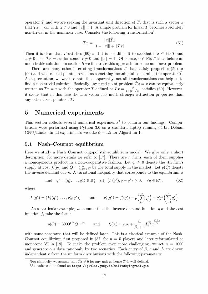
5.1 Nash–Cournot equilibriumHere we study a Nash–Cournot oligopolistic equilibrium model. We give only a shortdescription, for more details we refer to [17]. There are n firms, each of them suppliesa homogeneous product in a non-cooperative fashion. Let qi ≥ 0 denote the ith firm’ssupply at cost fi(qi) and Q = ∑n

i=1 qi be the total supply in the market. Let p(Q) denotethe inverse demand curve. A variational inequality that corresponds to the equilibrium is

find q∗ = (q∗1, . . . , q∗n) ∈ Rn+ s.t. 〈F (q∗), q − q∗〉 ≥ 0, ∀q ∈ Rn

+, (62)

where

F (q∗) = (F1(q∗), . . . , Fn(q∗)) and Fi(q∗) = f ′i(q∗i )− p( n∑j=1

q∗j

)− q∗i p′

( n∑j=1

q∗j

)

As a particular example, we assume that the inverse demand function p and the costfunction fi take the form:

p(Q) = 50001/γQ−1/γ and fi(qi) = ciqi + βiβi + 1L

1βii q

βi+1βi

i

with some constants that will be defined later. This is a classical example of the Nash-Cournot equilibrium first proposed in [37] for n = 5 players and later reformulated asmonotone VI in [19]. To make the problem even more challenging, we set n = 1000and generate our data randomly by two scenarios. Each entry of β, c and L are drawnindependently from the uniform distributions with the following parameters:

2For simplicity we assume that T̃ x 6= 0 for any unit x, hence T is well-defined.3All codes can be found on https://gitlab.gwdg.de/malitskyi/graal.git.

17

(a) γ = 1.1, βi ∼ U(0.5, 2), ci ∼ U(1, 100), Li ∼ U(0.5, 5);

(b) γ = 1.5, βi ∼ U(0.3, 4) and ci, Li as above.

Clearly, parameters β and γ are the most important as they control the level of smoothnessof fi and p. There are two main issues that make many existing algorithms not-applicableto this problem. The first is, of course, that due to the choice of β and γ, F is notLipschitz-continuous. The second is that F is defined only on Rn

+. This issue, which wasalready noticed in [47] for the case n = 10, makes the above problem difficult for thosealgorithms that compute F at the point which is a linear combination of the feasibleiterates. For example, the reflected projected gradient method evaluates F at 2xk−xk−1,which might not belong to the domain of F .

For each scenario above we generate 10 random instances and for comparison we usethe residual ‖q−PRn+(q−F (q))‖, which we compute in every iteration. The starting pointis z1 = (1, . . . , 1). We compare EGRAAL with Tseng’s FBF method with linesearch [52].The results are reported in Figure 1. One can see that EGRAAL substantially outperformsthe FBF method. Note that the latter method even without linesearch requires twoevaluations of F , so in terms of the CPU time that distinction would be even moresignificant.

0 2000 4000 6000 8000 10000iterations, k

10 12

10 10

10 8

10 6

10 4

10 2

100

102

resid

ual

FBFEGRAAL

0 10000 20000 30000 40000 50000iterations, k

10 12

10 10

10 8

10 6

10 4

10 2

100

102

resid

ual

FBFEGRAAL

Figure 1: Results for problem (62). Scenario (a) on the left, (b) on the right.

5.2 Convex feasibility problemGiven a number of closed convex sets Ci ∈ E , i = 1, . . . ,m, the convex feasibility problem(CFP) aims to find a point in their intersection: x ∈ ∩mi=1Ci. The problem is verygeneral and allows one to represent many practical problems in this form. Projectionmethods are a standard tool to solve such problem (we refer to [5,16] for a more in-depthoverview). In this note we study a simultaneous projection method: xk+1 = Txk, whereT = 1

m(PC1 + · · · + PCm). Its main advantage is that it can be easily implemented on a

parallel computing architecture. Although it might be slower than the cyclic projectionmethod xk+1 = PC1 . . . PCmx

k in terms of iterations, for large-scale problems it is oftenmuch faster in practice due to parallelization and more efficient ways of computing Tx.

One can look at the iteration xk+1 = Txk as an application of the Krasnoselskii-Mannscheme for the firmly-nonexpansive operator T . By that (xk) converges to a fixed pointof T , which is either a solution of CFP (consistent case) or a solution of the problemminx

∑mi=1 dist(x,Ci)2 (inconsistent case when the intersection is empty).

18

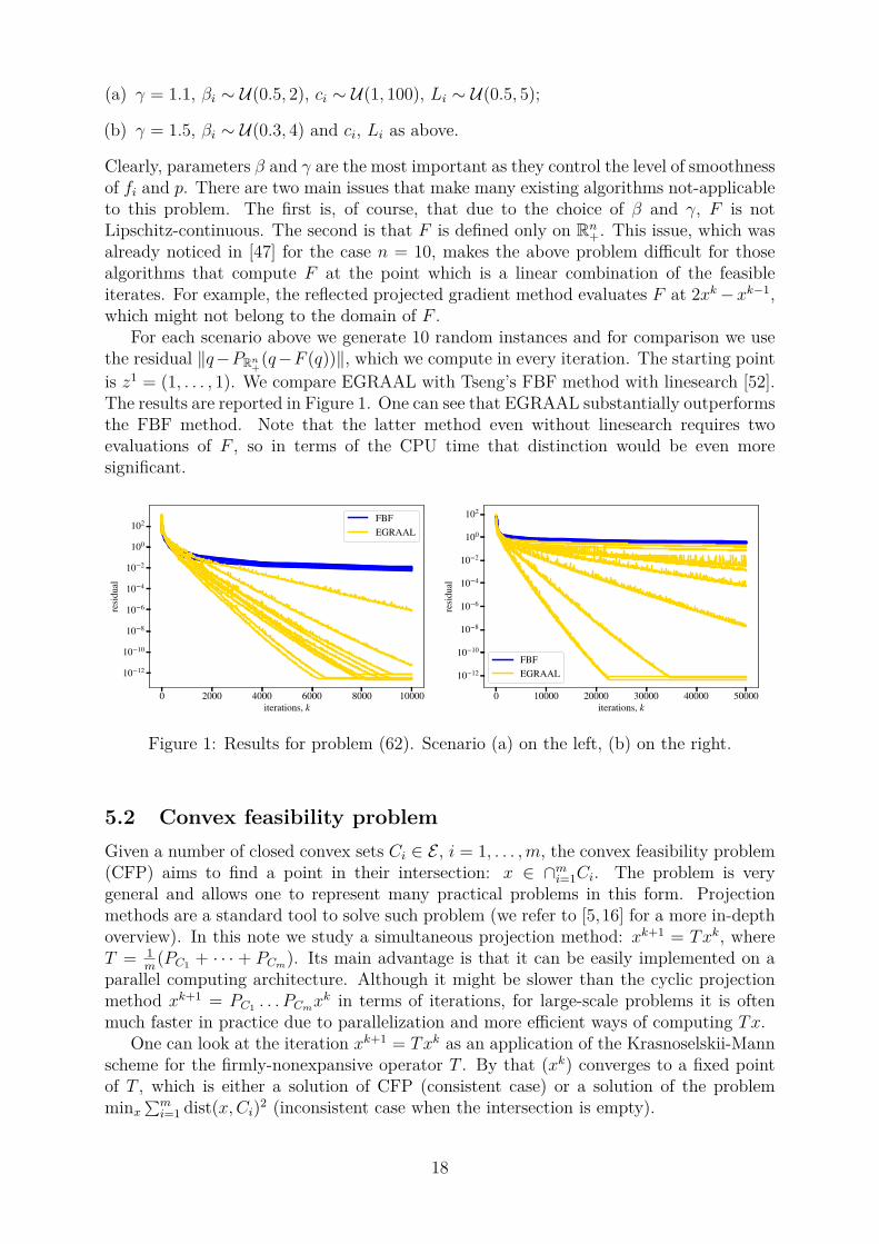
To illustrate Remark 3, we show how in many cases EGRAAL with F = Id−T canaccelerate convergence of the simultaneous projection algorithm. We believe, this is quiteinteresting, especially if one takes into account that our framework works as a black box:it does not require any tuning or a priori information about the initial problem.

Tomography reconstruction

The goal of the tomography reconstruction problem is to obtain a slice image of an objectfrom a set of projections (sinogram). Mathematically speaking, this is an instance of alinear inverse problem

Ax = b̂, (63)

where x ∈ Rn is the unknown image, A ∈ Rm×n is the projection matrix, and b̂ ∈ Rm

is the given sinogram. In practice, however, b̂ is contaminated by some noise ε ∈ Rm,so we observe only b = b̂ + ε. It is clear that we can formulate the given problem asCFP with Ci = {x : 〈ai, x〉 = bi}. However, since the projection matrix A is often rank-deficient, it is very likely that b /∈ range(A), thus we have to consider the inconsistentcase minx

∑mi=1 dist(x,Ci)2. As the projection onto Ci is given by PCix = x − 〈ai,x〉−bi‖ai‖2 ai,

computing Tx reduces to the matrix-vector multiplications which is realized efficiently inmost computer processors. Note that our approach only exploits feasibility constraints,which is definitely not a state of the art model for tomography reconstruction. Moreinvolved methods would solve this problem with the use of some regularization techniques,but we keep such simple model for illustration purposes only.

As a particular problem, we wish to reconstruct the Shepp-Logan phantom image256 × 256 (thus, x ∈ Rn with n = 216) from the far less measurements m = 215. Wegenerate the matrix A ∈ Rm×n from the scikit-learn library and define b = Ax + ε,where ε ∈ Rm is a random vector, whose entries are drawn from N (0, 1). The startingpoint was chosen as x1 = (0, . . . , 0) and λ0 = 1. In Figure 2 (left) we report how theresidual ‖xk−Txk‖ is changing w.r.t. the number of iterations and in Figure 2 (right) weshow the size of steps for EGRAAL scheme. Recall that the CPU time of both is almostthe same, so one can reliably state that in this case EGRAAL in fact accelerates the fixedpoint iteration xk+1 = Txk. The information about the steps λk gives us at least someexplanation of what we observe: with larger λk the role of Txk in (40) increases and hencewe are faster approaching to the fixed point set.

0 200 400 600 800 1000iterations, k

10 4

10 3

10 2

10 1

resid

ual

KM: xk + 1 = Txk

EGRAAL

0 200 400 600 800 1000iterations, k

0

500

1000

1500

2000

2500

steps

ize k

EGRAAL

Figure 2: Results for problem (63). Left: the behavior of residual ‖xk − Txk‖ for KMand EGRAAL methods. Right: the size of stepsize of λk for EGRAAL

19

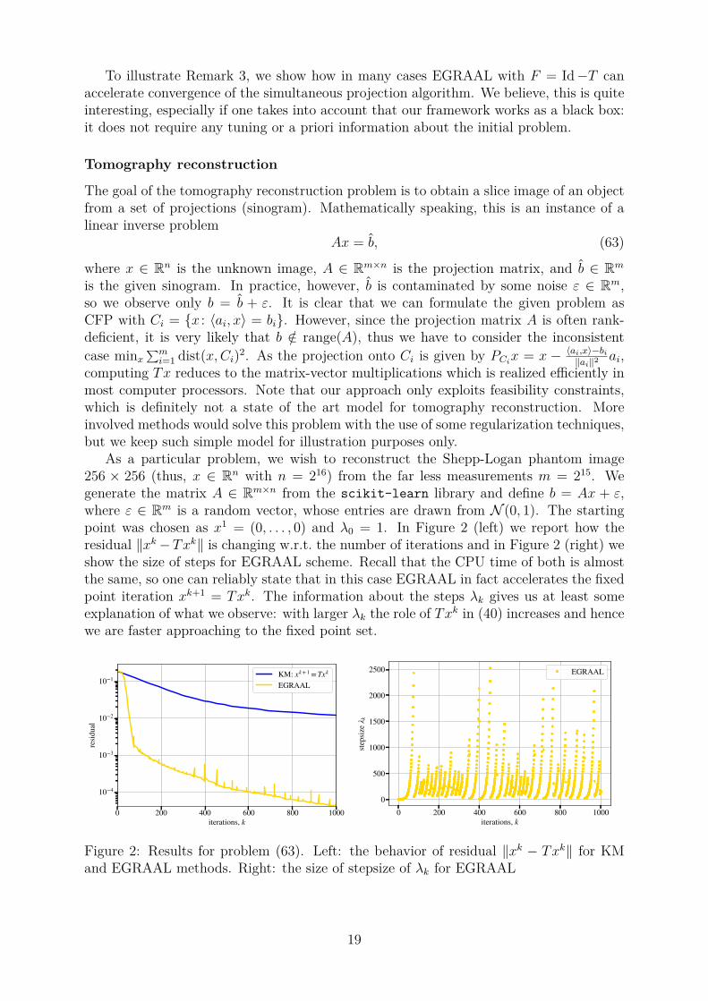
Intersection of balls

Now we consider a synthetic nonlinear feasibility problem. We have to find a point inx ∈ ∩mi=1Ci, where Ci = B(ci, ri), a closed ball with a center ci ∈ Rn and a radius ri > 0.The projection onto Ci is simple: PCix equals to x−ci

‖x−ci‖ri if ‖x− ci‖ > ri and x otherwise.Thus, again computing Tx = 1

m

∑mi=1 PCix can be done in parallel very efficiently.

We run two scenarios: with n = 1000, m = 2000 and with n = 2000, m = 1000. Eachcoordinate of ci ∈ Rn is drawn from N (0, 100). Then we set ri = ‖ci‖ + 1 that ensuresthat zero belongs to the intersection of Ci. The starting point was chosen as the averageof all centers: x1 = 1

m

∑mi=1 ci. As before, since the cost of iteration of both methods is

approximately the same, we show only how the residual ‖Txk−xk‖ is changing w.r.t. thenumber of iterations. To eliminate the role of chance, we plot the results for 100 randomrealizations from each of the above scenarios. Figure 3 depicts the results. As one cansee, the difference is again significant.

0 200 400 600 800 1000iterations, k

10 13

10 11

10 9

10 7

10 5

10 3

10 1

resid

ual

KMEGRAAL

0 200 400 600 800 1000iterations, k

10 13

10 11

10 9

10 7

10 5

10 3

10 1

resid

ual

KMEGRAAL

Figure 3: Convergence results for CFP with random balls Ci. T = 1m

∑mi=1 PCi . Left:

n = 1000, m = 2000. Right: n = 2000, m = 1000.

5.3 Sparse logistic regressionIn this section we demonstrate that even for nice problems as composite minimization (3)with Lipschitz ∇f , EGRAAL can be faster than the proximal gradient method or accel-erated proximal gradient method. This is interesting, especially since the latter methodhas a better theoretical convergence rate.

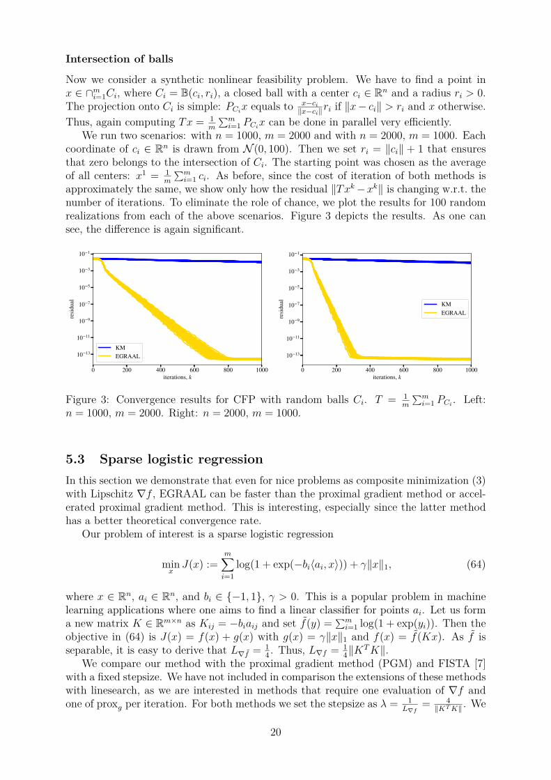
Our problem of interest is a sparse logistic regression

minxJ(x) :=

m∑i=1

log(1 + exp(−bi〈ai, x〉)) + γ‖x‖1, (64)

where x ∈ Rn, ai ∈ Rn, and bi ∈ {−1, 1}, γ > 0. This is a popular problem in machinelearning applications where one aims to find a linear classifier for points ai. Let us forma new matrix K ∈ Rm×n as Kij = −biaij and set f̃(y) = ∑m

i=1 log(1 + exp(yi)). Then theobjective in (64) is J(x) = f(x) + g(x) with g(x) = γ‖x‖1 and f(x) = f̃(Kx). As f̃ isseparable, it is easy to derive that L∇f̃ = 1

4 . Thus, L∇f = 14‖K

TK‖.We compare our method with the proximal gradient method (PGM) and FISTA [7]

with a fixed stepsize. We have not included in comparison the extensions of these methodswith linesearch, as we are interested in methods that require one evaluation of ∇f andone of proxg per iteration. For both methods we set the stepsize as λ = 1

L∇f= 4‖KTK‖ . We

20

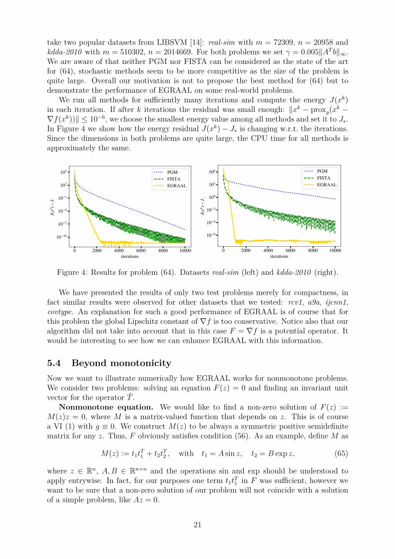
take two popular datasets from LIBSVM [14]: real-sim with m = 72309, n = 20958 andkdda-2010 with m = 510302, n = 2014669. For both problems we set γ = 0.005‖AT b‖∞.We are aware of that neither PGM nor FISTA can be considered as the state of the artfor (64), stochastic methods seem to be more competitive as the size of the problem isquite large. Overall our motivation is not to propose the best method for (64) but todemonstrate the performance of EGRAAL on some real-world problems.

We run all methods for sufficiently many iterations and compute the energy J(xk)in each iteration. If after k iterations the residual was small enough: ‖xk − proxg(xk −∇f(xk))‖ ≤ 10−6, we choose the smallest energy value among all methods and set it to J∗.In Figure 4 we show how the energy residual J(xk)− J∗ is changing w.r.t. the iterations.Since the dimensions in both problems are quite large, the CPU time for all methods isapproximately the same.

0 2000 4000 6000 8000 10000iterations

10 10

10 7

10 4

10 1

102

105

J(xk )

J *

PGMFISTAEGRAAL

0 2000 4000 6000 8000 10000iterations

10 9

10 6

10 3

100

103

106

J(xk )

J *

PGMFISTAEGRAAL

Figure 4: Results for problem (64). Datasets real-sim (left) and kdda-2010 (right).

We have presented the results of only two test problems merely for compactness, infact similar results were observed for other datasets that we tested: rcv1, a9a, ijcnn1,covtype. An explanation for such a good performance of EGRAAL is of course that forthis problem the global Lipschitz constant of ∇f is too conservative. Notice also that ouralgorithm did not take into account that in this case F = ∇f is a potential operator. Itwould be interesting to see how we can enhance EGRAAL with this information.

5.4 Beyond monotonicityNow we want to illustrate numerically how EGRAAL works for nonmonotone problems.We consider two problems: solving an equation F (z) = 0 and finding an invariant unitvector for the operator T̃ .

Nonmonotone equation. We would like to find a non-zero solution of F (z) :=M(z)z = 0, where M is a matrix-valued function that depends on z. This is of coursea VI (1) with g ≡ 0. We construct M(z) to be always a symmetric positive semidefinitematrix for any z. Thus, F obviously satisfies condition (56). As an example, define M as

M(z) := t1tT1 + t2t

T2 , with t1 = A sin z, t2 = B exp z, (65)

where z ∈ Rn, A,B ∈ Rn×n and the operations sin and exp should be understood toapply entrywise. In fact, for our purposes one term t1t

T1 in F was sufficient, however we

want to be sure that a non-zero solution of our problem will not coincide with a solutionof a simple problem, like Az = 0.

21

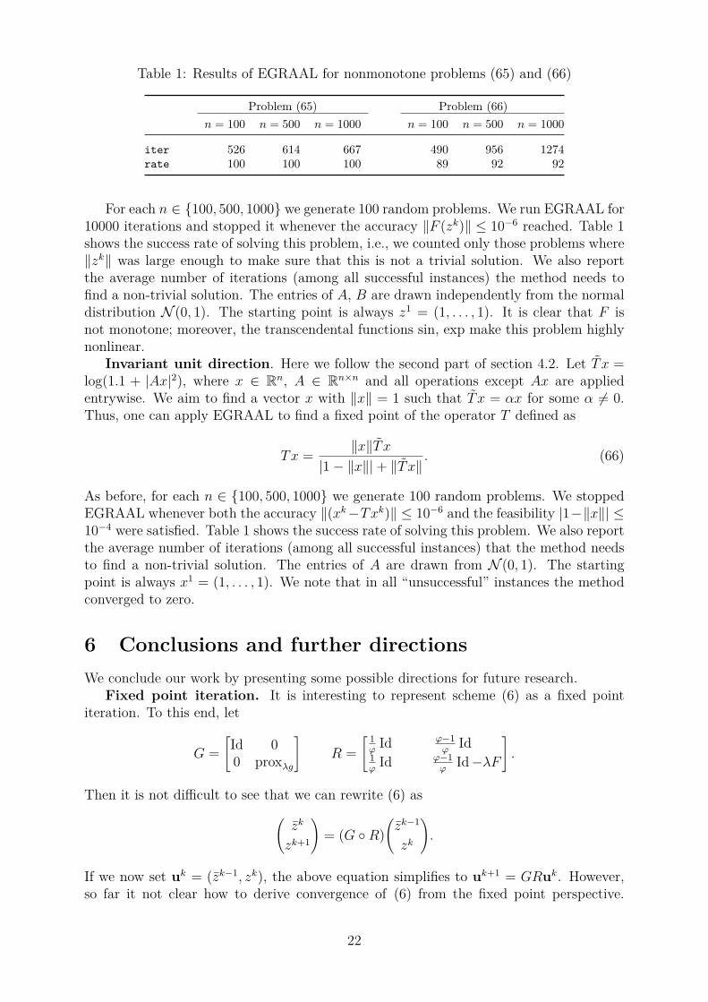
Table 1: Results of EGRAAL for nonmonotone problems (65) and (66)

Problem (65) Problem (66)n = 100 n = 500 n = 1000 n = 100 n = 500 n = 1000

iter 526 614 667 490 956 1274rate 100 100 100 89 92 92

For each n ∈ {100, 500, 1000} we generate 100 random problems. We run EGRAAL for10000 iterations and stopped it whenever the accuracy ‖F (zk)‖ ≤ 10−6 reached. Table 1shows the success rate of solving this problem, i.e., we counted only those problems where‖zk‖ was large enough to make sure that this is not a trivial solution. We also reportthe average number of iterations (among all successful instances) the method needs tofind a non-trivial solution. The entries of A, B are drawn independently from the normaldistribution N (0, 1). The starting point is always z1 = (1, . . . , 1). It is clear that F isnot monotone; moreover, the transcendental functions sin, exp make this problem highlynonlinear.

Invariant unit direction. Here we follow the second part of section 4.2. Let T̃ x =log(1.1 + |Ax|2), where x ∈ Rn, A ∈ Rn×n and all operations except Ax are appliedentrywise. We aim to find a vector x with ‖x‖ = 1 such that T̃ x = αx for some α 6= 0.Thus, one can apply EGRAAL to find a fixed point of the operator T defined as

Tx = ‖x‖T̃ x|1− ‖x‖|+ ‖T̃ x‖

. (66)

As before, for each n ∈ {100, 500, 1000} we generate 100 random problems. We stoppedEGRAAL whenever both the accuracy ‖(xk−Txk)‖ ≤ 10−6 and the feasibility |1−‖x‖| ≤10−4 were satisfied. Table 1 shows the success rate of solving this problem. We also reportthe average number of iterations (among all successful instances) that the method needsto find a non-trivial solution. The entries of A are drawn from N (0, 1). The startingpoint is always x1 = (1, . . . , 1). We note that in all “unsuccessful” instances the methodconverged to zero.

6 Conclusions and further directionsWe conclude our work by presenting some possible directions for future research.

Fixed point iteration. It is interesting to represent scheme (6) as a fixed pointiteration. To this end, let

G =[Id 00 proxλg

]R =

[ 1ϕ

Id ϕ−1ϕ

Id1ϕ

Id ϕ−1ϕ

Id−λF

].

Then it is not difficult to see that we can rewrite (6) as(z̄k

zk+1

)= (G ◦R)

(z̄k−1

zk

).

If we now set uk = (z̄k−1, zk), the above equation simplifies to uk+1 = GRuk. However,so far it not clear how to derive convergence of (6) from the fixed point perspective.

22

Although, G is a firmly-nonexpansive operator, R is definitely not; thus, it is difficult tosay something meaningful about G ◦R.

Inertial extensions. Starting from the paper [43], it is observed that using someinertia for the optimization algorithm often accelerates the latter. Later, papers [1,10,28,36] extend this idea to a more general case with monotone operators. In our case it willbe in particular interesting to do so, since our scheme

zk+1 = proxλg(z̄k − λF (zk))

uses z̄k as a convex combination of all previous iterates z1 . . . , zk. This is completelyopposite to the inertial methods, where one uses zk + α(zk − zk−1) for some α > 0.

Bregman distance. For many VI methods it is possible to derive their analogues forthe Bregman distances, as this is done for the the extragradient method [27] by extensions[39,41]. It is possible to do so for GRAAL? This extension is not trivial since, for example,in (12) we have used the identity (5), where the linear structure was explicitly used.

Stochastic settings. For large-scale problems it is often the case that even computingF (zk) becomes prohibitively expensive. For this reason, the stochastic VI methods thatcompute F (zk) approximately can be advantageous over their deterministic counterparts,as it was shown in [3, 23]. It is interesting to derive similar extensions for GRAAL. Thesame concerns to the coordinate extensions of GRAAL.

Nonmonotone case. There are more things here that are not known that known.As it was already mentioned, it is important to understand the behavior of EGRAAL atleast for some nonmonotone problems: when it converges to a non-trivial solution, i.e.,what is the basin of attraction for the discrete dynamical system provided by EGRAAL?From the practical point of view, it is also important to find some real world problemswhere EGRAAL can be applied.

Acknowledgments: This research was supported by the German Research Foundationgrant SFB755-A4. The author is very grateful to Matthew Tam and Anna–Lena Martinsfor their valuable comments.

References[1] F. Alvarez and H. Attouch. An inertial proximal method for maximal monotone op-

erators via discretization of a nonlinear oscillator with damping. Set-Valued Analysis,9(1-2):3–11, 2001.

[2] K. J. Arrow, L. Hurwicz, and H. Uzawa. Studies in linear and non-linear program-ming. Stanford University Press, 1958.

[3] M. Baes, M. Bürgisser, and A. Nemirovski. A randomized mirror-prox method forsolving structured large-scale matrix saddle-point problems. SIAM Journal on Op-timization, 23(2):934–962, 2013.

[4] H. H. Bauschke, J. Bolte, and M. Teboulle. A descent lemma beyond Lipschitzgradient continuity: first-order methods revisited and applications. Mathematics ofOperations Research, 2016.

[5] H. H. Bauschke and J. M. Borwein. On projection algorithms for solving convexfeasibility problems. SIAM Review, 38(3):367–426, 1996.

23

[6] H. H. Bauschke and P. L. Combettes. Convex Analysis and Monotone OperatorTheory in Hilbert Spaces. Springer, New York, 2011.

[7] A. Beck and M. Teboulle. A fast iterative shrinkage-thresholding algorithm for linearinverse problem. SIAM Journal on Imaging Sciences, 2(1):183–202, 2009.

[8] J. Bello Cruz and R. Díaz Millán. A variant of forward-backward splitting methodfor the sum of two monotone operators with a new search strategy. Optimization,64(7):1471–1486, 2015.

[9] V. Berinde. Iterative approximation of fixed points, volume 1912. Springer, 2007.

[10] R. I. Boţ and E. R. Csetnek. An inertial forward-backward-forward primal-dualsplitting algorithm for solving monotone inclusion problems. Numerical Algorithms,71(3):519–540, 2016.

[11] Y. Censor, A. Gibali, and S. Reich. The subgradient extragradient method for solv-ing variational inequalities in Hilbert space. Journal of Optitmization Theory andApplications, 148:318–335, 2011.

[12] A. Chambolle and T. Pock. A first-order primal-dual algorithm for convex prob-lems with applications to imaging. Journal of Mathematical Imaging and Vision,40(1):120–145, 2011.

[13] A. Chambolle and T. Pock. On the ergodic convergence rates of a first-order primal–dual algorithm. Mathematical Programming, pages 1–35, 2015.

[14] C.-C. Chang and C.-J. Lin. LIBSVM: a library for support vector machines. ACMtransactions on intelligent systems and technology (TIST), 2(3):27, 2011.

[15] G. H. Chen and R. T. Rockafellar. Convergence rates in forward–backward splitting.SIAM Journal on Optimization, 7(2):421–444, 1997.

[16] P. Combettes. The convex feasibility problem in image recovery. Advances in imagingand electron physics, 95:155–270, 1996.

[17] F. Facchinei and J.-S. Pang. Finite-Dimensional Variational Inequalities and Com-plementarity Problems, Volume I and Volume II. Springer-Verlag, New York, USA,2003.

[18] P. Giselsson, M. Fält, and S. Boyd. Line search for averaged operator iteration.In Decision and Control (CDC), 2016 IEEE 55th Conference on, pages 1015–1022.IEEE, 2016.

[19] P. T. Harker. A variational inequality approach for the determination of oligopolisticmarket equilibrium. Mathematical Programming, 30(1):105–111, 1984.

[20] B. He. A new method for a class of linear variational inequalities. MathematicalProgramming, 66(1-3):137–144, 1994.

[21] S. Ishikawa. Fixed points by a new iteration method. Proceedings of the AmericanMathematical Society, 44(1):147–150, 1974.

24

[22] A. N. Iusem and B. F. Svaiter. A variant of Korpelevich’s method for variationalinequalities with a new search strategy. Optimization, 42:309–321, 1997.

[23] A. Juditsky, A. Nemirovski, and C. Tauvel. Solving variational inequalities withstochastic mirror-prox algorithm. Stochastic Systems, 1(1):17–58, 2011.

[24] E. N. Khobotov. Modification of the extragradient method for solving variationalinequalities and certain optimization problems. USSR Computational Mathematicsand Mathematical Physics, 27:120–127, 1989.

[25] D. Kinderlehrer and G. Stampacchia. An introduction to variational inequalities andtheir applications, volume 31. SIAM, 1980.

[26] I. Konnov. A class of combined iterative methods for solving variational inequalities.Journal of Optimization Theory and Applications, 94(3):677–693, 1997.

[27] G. M. Korpelevich. The extragradient method for finding saddle points and otherproblems. Ekonomika i Matematicheskie Metody, 12(4):747–756, 1976.

[28] D. Lorenz and T. Pock. An inertial forward-backward algorithm for monotone inclu-sions. Journal of Mathematical Imaging and Vision, 51(2):311–325, 2015.

[29] H. Lu, R. M. Freund, and Y. Nesterov. Relatively smooth convex optimization byfirst-order methods, and applications. SIAM Journal on Optimization, 28(1):333–354, 2018.

[30] D. R. Luke, N. H. Thao, and M. K. Tam. Quantitative convergence analysis ofiterated expansive, set-valued mappings. arXiv preprint arXiv:1605.05725, 2016.

[31] S. I. Lyashko, V. V. Semenov, and T. A. Voitova. Low-cost modification of Ko-rpelevich’s method for monotone equilibrium problems. Cybernetics and SystemsAnalysis, 47:631–639, 2011.

[32] Y. Malitsky. Reflected projected gradient method for solving monotone variationalinequalities. SIAM Journal on Optimization, 25(1):502–520, 2015.

[33] Y. Malitsky. Proximal extrapolated gradient methods for variational inequalities.Optimization Methods and Software, 33(1):140–164, 2018.

[34] Y. V. Malitsky and V. V. Semenov. An extragradient algorithm for monotone vari-ational inequalities. Cybernetics and Systems Analysis, 50(2):271–277, 2014.

[35] R. D. Monteiro and B. F. Svaiter. Complexity of variants of Tseng’s modified FBsplitting and Korpelevich’s methods for hemivariational inequalities with applicationsto saddle-point and convex optimization problems. SIAM Journal on Optimization,21(4):1688–1720, 2011.

[36] A. Moudafi and M. Oliny. Convergence of a splitting inertial proximal methodfor monotone operators. Journal of Computational and Applied Mathematics,155(2):447–454, 2003.

[37] F. H. Murphy, H. D. Sherali, and A. L. Soyster. A mathematical programming ap-proach for determining oligopolistic market equilibrium. Mathematical Programming,24(1):92–106, 1982.

25

[38] S. Naimpally and K. Singh. Extensions of some fixed point theorems of rhoades.Journal of mathematical analysis and applications, 96(2):437–446, 1983.

[39] A. Nemirovski. Prox-method with rate of convergence o(1/t) for variational inequali-ties with lipschitz continuous monotone operators and smooth convex-concave saddlepoint problems. SIAM Journal on Optimization, 15(1):229–251, 2004.

[40] A. Nemirovsky. Information-based complexity of linear operator equations. Journalof Complexity, 8(2):153–175, 1992.

[41] Y. Nesterov. Dual extrapolation and its applications to solving variational inequali-ties and related problems. Mathematical Programming, 109(2-3):319–344, 2007.

[42] J.-S. Pang. Error bounds in mathematical programming. Mathematical Programming,79(1-3):299–332, 1997.

[43] B. Polyak. Some methods of speeding up the convergence of iteration methods.U.S.S.R. Computational Mathematics and Mathematical Physics, 4(5):1–17, 1967.

[44] L. D. Popov. A modification of the Arrow-Hurwicz method for finding saddle points.Mathematical Notes, 28(5):845–848, 1980.

[45] L. Qihou. On Naimpally and Singh’s open questions. Journal of mathematical anal-ysis and applications, 124(1):157–164, 1987.

[46] M. V. Solodov. Convergence rate analysis of iteractive algorithms for solving varia-tional inequality problems. Mathematical Programming, 96(3):513–528, 2003.

[47] M. V. Solodov and B. F. Svaiter. A new projection method for variational inequalityproblems. SIAM Journal on Control and Optimization, 37(3):765–776, 1999.

[48] M. V. Solodov and P. Tseng. Modified projection-type methods for monotone vari-ational inequalities. SIAM Journal on Control and Optimization, 34(5):1814–1830,1996.

[49] A. Themelis and P. Patrinos. Supermann: a superlinearly convergent algorithm forfinding fixed points of nonexpansive operators. arXiv preprint arXiv:1609.06955,2016.

[50] Q. Tran-Dinh, A. Kyrillidis, and V. Cevher. Composite self-concordant minimization.The Journal of Machine Learning Research, 16(1):371–416, 2015.

[51] P. Tseng. On linear convergence of iterative methods for the variational inequalityproblem. Journal of Computational and Applied Mathematics, 60(1-2):237–252, 1995.

[52] P. Tseng. A modified forward-backward splitting method for maximal monotonemappings. SIAM Journal on Control and Optimization, 38:431–446, 2000.

26