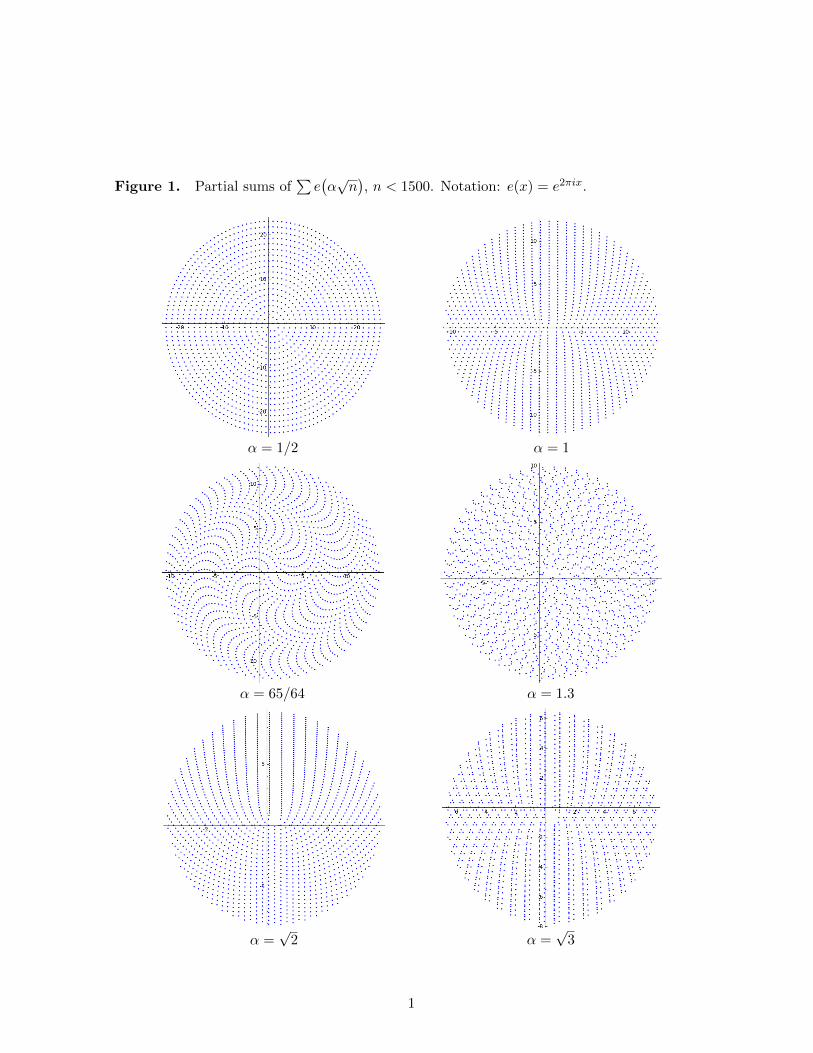
Figure 1. Partial sums of∑e(α√n), n < 1500. Notation: e(x) = e2πix.

α = 1/2 α = 1

α = 65/64 α = 1.3

α =√2 α =

√3

1

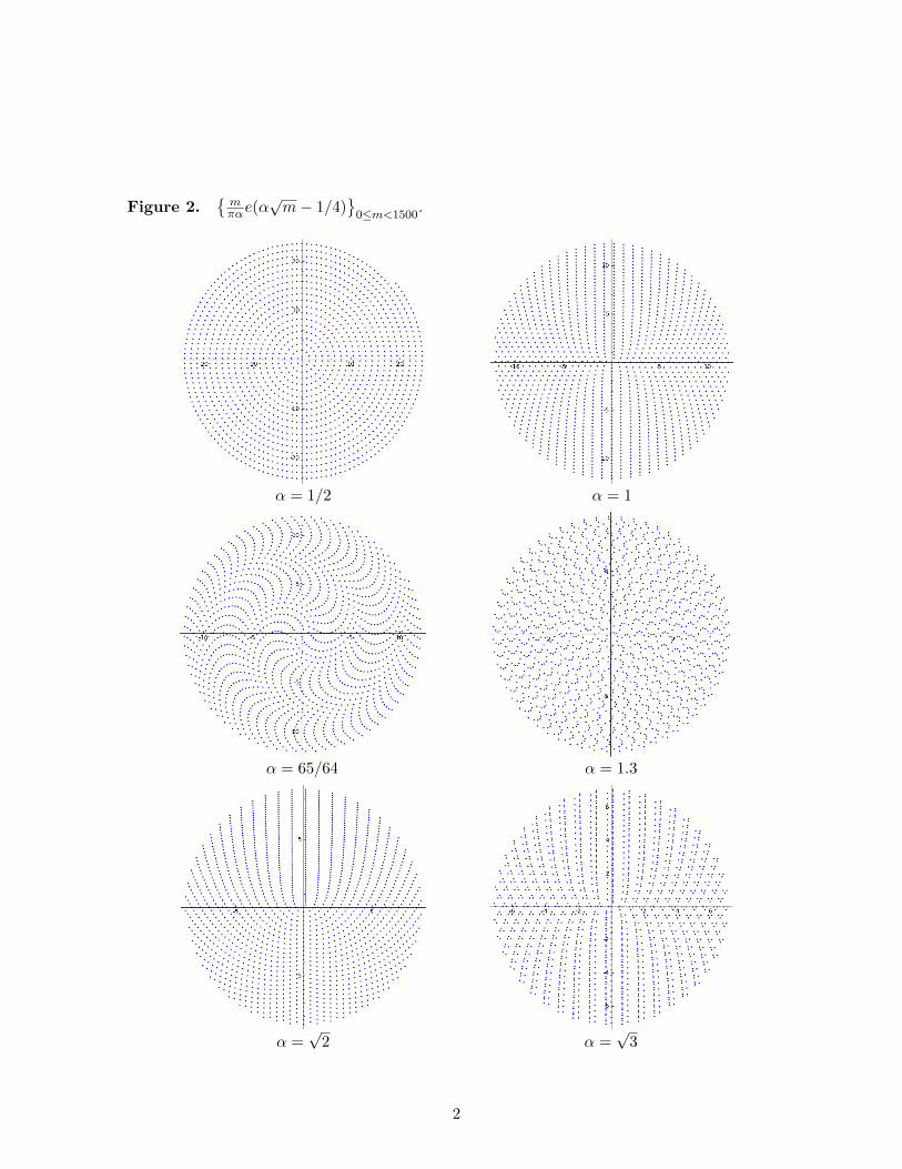
Figure 2.{mπαe(α

√m− 1/4)

}0≤m<1500

.

α = 1/2 α = 1

α = 65/64 α = 1.3

α =√2 α =

√3

2

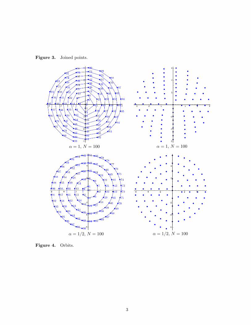
Figure 3. Joined points.

α = 1, N = 100 α = 1, N = 100

α = 1/2, N = 100 α = 1/2, N = 100

Figure 4. Orbits.

3

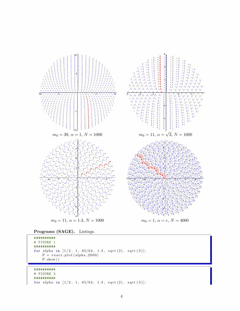
m0 = 39, α = 1, N = 1000 m0 = 11, α =√3, N = 1000

m0 = 11, α = 1.3, N = 1000 m0 = 1, α = e, N = 4000

Programs (SAGE). Listings.

##########

# FIGURE 1

##########

for alpha in [ 1 /2 , 1 , 65/64 , 1 . 3 , s q r t ( 2 ) , s q r t ( 3 ) ] :P = exa c t p l o t ( alpha ,2000 )P. show ( )

##########

# FIGURE 2

##########

for alpha in [ 1 /2 , 1 , 65/64 , 1 . 3 , s q r t ( 2 ) , s q r t ( 3 ) ] :

4

P = plot mode l ( alpha ,2000 )P. show ( )

##########

# FIGURE 3

##########

P = p lo t mode l t j (1/2 ,100)P. show ( )P = plot mode l (1/2 ,100 , 40)P. show ( )P = p lo t mode l t j (1 ,100)P. show ( )P = plot mode l (1 ,100 , 40)P. show ( )

##########

# FIGURE 4

##########

P = orb i t (39 , 1 , 1000 , p s i z e = 15)P. show ( )P = o rb i t (11 , s q r t ( 3 ) , 1000 , p s i z e = 15)P. show ( )P = o rb i t (11 , 1 . 3 , 1000 , p s i z e = 15)P. show ( )P = o rb i t (1 , exp (1 ) , 4000 , p s i z e = 10)P. show ( )

%cythonimport mathdef l s q r ( double alpha , long long i n t N) :

cde f double sx = 0 .0cde f double sy = 0 .0cde f double tcde f double nLt = [ ]for n in range (N) :

t = 6.28318530717958647692528∗ alpha ∗math . sq r t (n)sx += math . cos ( t )sy += math . s i n ( t )Lt . append ( ( sx , sy ) )

return Lt

# exact calculations

def e xa c t p l o t ( alph , n po in t s ) :L = l s q r ( alph , n po in t s )P = l i s t p l o t (L , s i z e = 5)P. s e t a s p e c t r a t i o (1 )return P

# model

def plot mode l ( alph , n po ints , p s i z e = 5 ) :L = [ ]for k in range ( n po in t s ) :

5

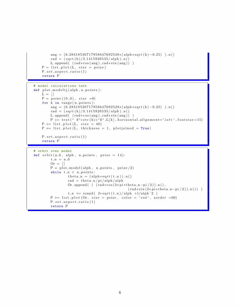
ang = (6.28318530717958647692528∗( alph ∗ s q r t ( k )−0.25) ) . n ( )rad = ( sq r t ( k )/3.1415926535/ alph ) . n ( )L . append ( ( rad∗ cos ( ang ) , rad∗ s i n ( ang ) ) )

P = l i s t p l o t (L , s i z e = p s i z e )P. s e t a s p e c t r a t i o (1 )return P

# model calculations text

def p l o t mode l t j ( alph , n po in t s ) :L = [ ]P = point ( ( 0 , 0 ) , s i z e =0)for k in range ( n po in t s ) :

ang = (6.28318530717958647692528∗( alph ∗ s q r t ( k )−0.25) ) . n ( )rad = ( sq r t ( k )/3.1415926535/ alph ) . n ( )L . append ( ( rad∗ cos ( ang ) , rad∗ s i n ( ang ) ) )P += text (" $"+s t r ( k)+"$" ,L [ k ] , ho r i z on ta l a l i gnment=’left’ , f o n t s i z e =15)

P += l i s t p l o t (L , s i z e = 40)P += l i s t p l o t (L , th i c kne s s = 1 , p l o t j o i n ed = True )

P. s e t a s p e c t r a t i o (1 )return P

# orbit over model

def o rb i t ( n 0 , alph , n po ints , p s i z e = 14 ) :t n = n 0Or = [ ]P = plot mode l ( alph , n po ints , p s i z e /2)while t n < n po in t s :

theta n = ( alph ∗ s q r t ( t n ) ) . n ( )rad = theta n / p i / alph / alphOr . append ( ( ( rad∗ cos (2∗ pi ∗ theta n−pi / 2 ) ) . n ( ) ,

( rad∗ s i n (2∗ pi ∗ theta n−pi / 2 ) ) . n ( ) ) )t n += round ( 2∗ s q r t ( t n )/ alph +1/alph ˆ2 )

P += l i s t p l o t (Or , s i z e = ps i ze , c o l o r = ’red’ , zo rder =60)P. s e t a s p e c t r a t i o (1 )return P

6