Probability Theory

Review of essential concepts

Probability P(A B) = P(A) + P(B) – P(A B) 0 ≤ P(A) ≤ 1 P(Ω)=1

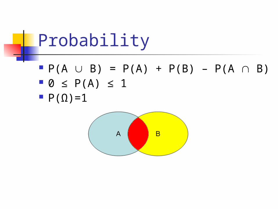
Problem 1 Given that P(A)=0.6 and P(B)=0.7,

which of the following cannot be true?

P(A B) = 0.5 = or P(A B) = 0.9 = and P(A B) = 0.2 P(A B) = 0.4 P(A B) = 0.7

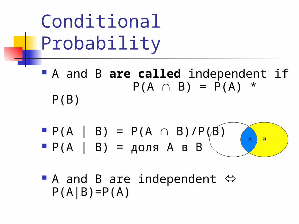
Conditional Probability A and B are called independent if

P(A B) = P(A) * P(B)

P(A | B) = P(A B)/P(B) P(A | B) = доля A в B

A and B are independent P(A|B)=P(A)

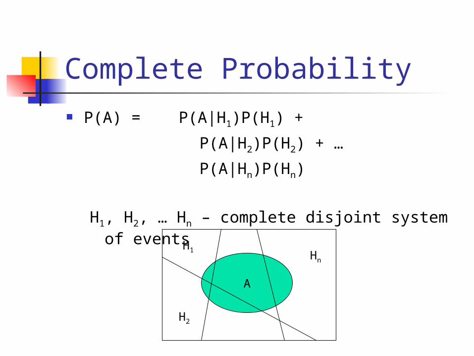
Complete Probability P(A) = P(A|H1)P(H1) +

P(A|H2)P(H2) + …

P(A|Hn)P(Hn)

H1, H2, … Hn – complete disjoint system of events

A

H1

H2

Hn

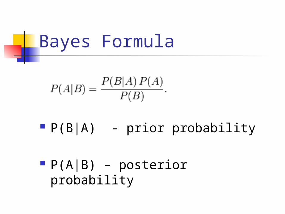
Bayes Formula

P(B|A) - prior probability

P(A|B) – posterior probability

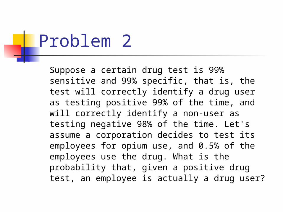
Problem 2

Suppose a certain drug test is 99% sensitive and 99% specific, that is, the test will correctly identify a drug user as testing positive 99% of the time, and will correctly identify a non-user as testing negative 98% of the time. Let's assume a corporation decides to test its employees for opium use, and 0.5% of the employees use the drug. What is the probability that, given a positive drug test, an employee is actually a drug user?

Problem 3

We are presented with three doors - red, green, and blue - one of which has a prize. We choose the red door, which is not opened until the presenter performs an action. The presenter who knows what door the prize is behind, and who must open a door, but is not permitted to open the door we have picked or the door with the prize, opens the blue door and reveals that there is no prize behind it and subsequently asks if we wish to change our mind about our initial selection of red. What is the probability that the prize is behind each of the green and red doors?

Random Variables Discrete (Uniform, Binomial, Poisson,

Geometric, Hypergeometric, Negative Binomial,…)

Continuous (Uniform, Normal, Exponential, Gamma, Chi-square, Student, Fisher, Dirchilet,…)

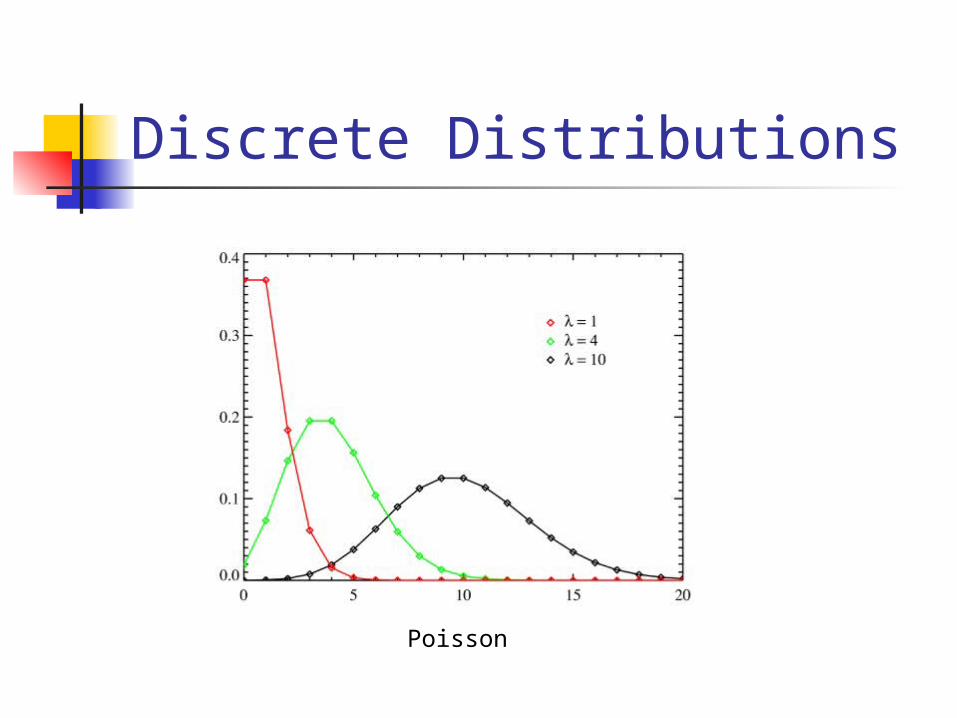
Discrete Distributions

Poisson

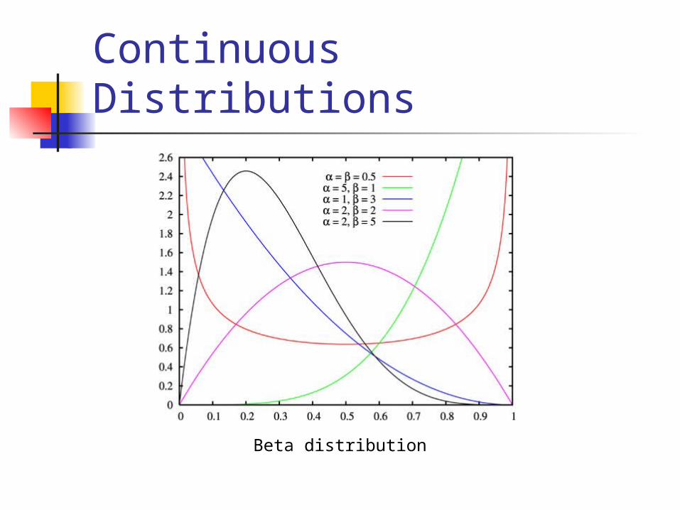
Continuous Distributions

Beta distribution

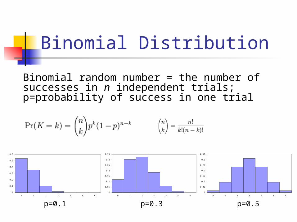
Binomial Distribution

Binomial random number = the number of successes in n independent trials; p=probability of success in one trial

0

0.1

0.2

0.3

0.4

0.5

0.6

0 1 2 3 4 5 6

0

0.05

0.1

0.15

0.2

0.25

0.3

0.35

0 1 2 3 4 5 6

0

0.05

0.1

0.15

0.2

0.25

0.3

0.35

0 1 2 3 4 5 6

p=0.1 p=0.3 p=0.5

Problem 4

The probability that a certain machine will

produce a defective item is 0.20. If a random

sample of 6 items is taken from the output of

this machine, what is the probability that

there will be 5 or more defectives in the

sample?

Problem 5There are 10 patients on the Neo-Natal Ward of

a local hospital who are monitored by 2 staff

members. If the probability (at any one time) of a

patient requiring emergency attention by a staff

member is 0.3, assuming the patients to be

behave independently, what is the probability at

any one time that there will not be sufficient staff

to attend all emergencies?

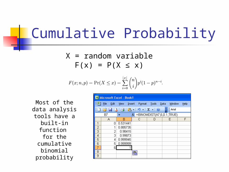
Cumulative Probability

X = random variableF(x) = P(X ≤ x)

Most of the data analysis tools have a built-in

function for the cumulative

binomial probability

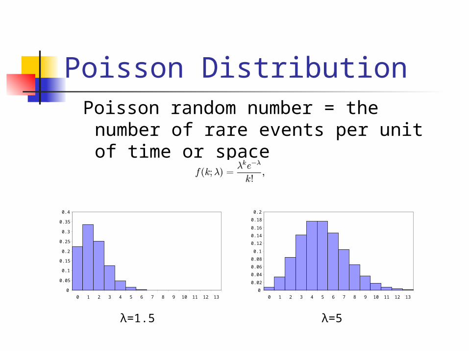
Poisson DistributionPoisson random number = the

number of rare events per unit of time or space

0

0.05

0.1

0.15

0.2

0.25

0.3

0.35

0.4

0 1 2 3 4 5 6 7 8 9 10 11 12 13

0

0.02

0.04

0.06

0.08

0.1

0.12

0.14

0.16

0.18

0.2

0 1 2 3 4 5 6 7 8 9 10 11 12 13

λ=1.5 λ=5

Problem 6

The marketing manager of a company has noted that she usually receives 10 complaint calls during a week (consisting of five working days), and that the calls occur at random. Find the probability that she gets five such calls in one day.

Problem 7 The rate at which a particular defect occurs

in lengths of plastic film being produced by a stable manufacturing process is 4.2 defects per 75 meter length. A random sample of the film is selected and it was found that the length of the film in the sample was 25 meters. What is the probability that there will be at most 2 defects found in the sample?

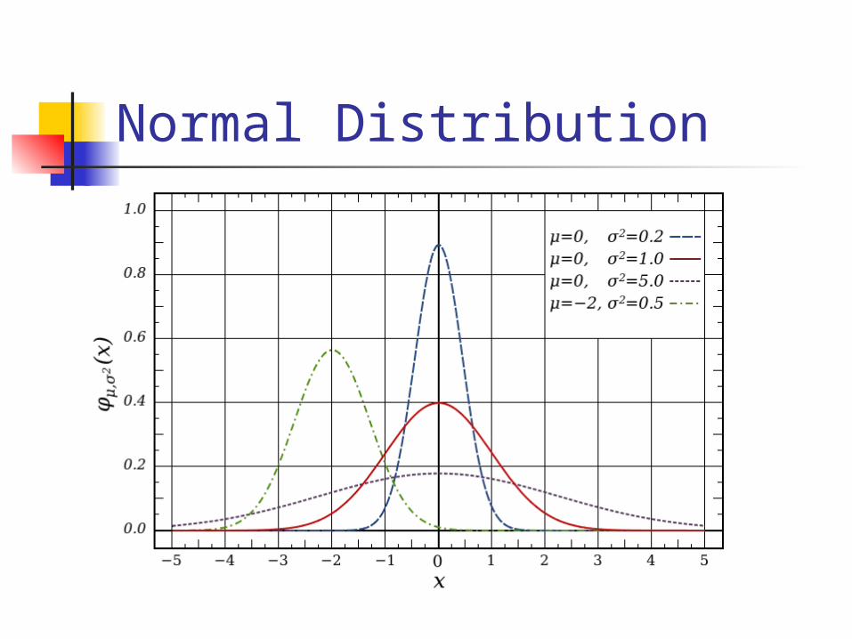
Normal Distribution

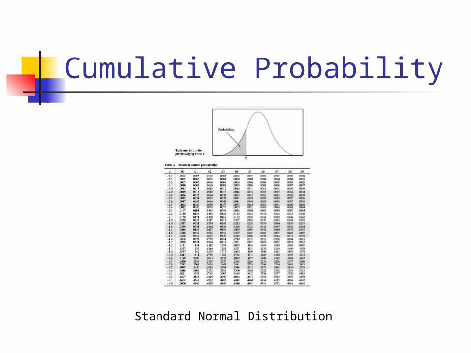
Cumulative Probability

Standard Normal Distribution

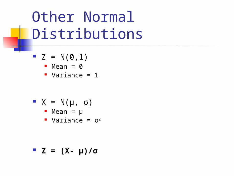
Other Normal Distributions Z = N(0,1)

Mean = 0 Variance = 1

X = N(μ, σ) Mean = μ Variance = σ2

Z = (X- μ)/σ

Problem 8

The diameters of steel disks produced in a plant are normally distributed with a mean of 2.5 cm and standard deviation of 0.02 cm. What is the probability that a disk picked at random has a diameter greater than 2.54 cm?

Problem 9

The height of an adult male is known to be normally distributed with a mean of 69 inches and a standard deviation of 2.5 inches. What is the height of the doorway such that 96 percent of the adult males can pass through it without having to bend?

Problem 10

The longevity of people living in a certain locality has a standard deviation of 14 years. What is the mean longevity if 30% of the people live longer than 75 years? Assume a normal distribution for life spans.

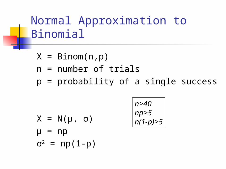
Normal Approximation to Binomial

X = Binom(n,p) n = number of trials p = probability of a single success

X = N(μ, σ) μ = np σ2 = np(1-p)

n>40np>5n(1-p)>5

Problem 11

The unemployment rate in a certain city is

8.5% . A random sample of 100 people from

the labor force is drawn. Find the approximate

probability that the sample contains at least

ten unemployed people.

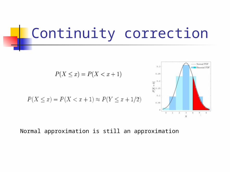
Continuity correction

Normal approximation is still an approximation

Problem 12Companies are interested in the demographics

of those who listen to the radio programs they

sponsor. A radio station has determined that

only 20% of listeners phoning in to a morning

talk program are male. During a particular

week, 200 calls are received by this program.

What is the approximate probability that at least

50 of the callers are male?

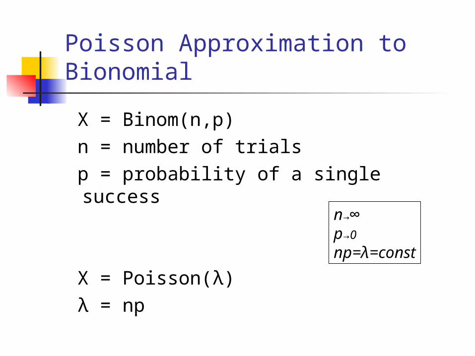
Poisson Approximation to Bionomial

X = Binom(n,p) n = number of trials p = probability of a single success

X = Poisson(λ) λ = np

n→∞p→0np=λ=const

Problem 13A certain genetic characteristic will

express itself in 0.001 of the population.

In a sample of n=3000 subjects, k=7 are

observed to display the characteristic,

whereas only three are expected to

display the characteristic. How likely is it

that a rate this great or greater could

occur by mere chance?

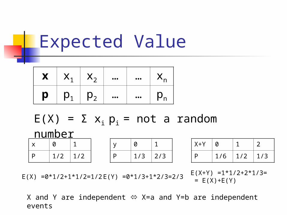
Expected Value

x x1 x2 … … xn

p p1 p2 … … pn

E(X) = Σ xi pi = not a random number

x 0 1

P 1/2 1/2

E(X) =0*1/2+1*1/2=1/2

y 0 1

P 1/3 2/3

E(Y) =0*1/3+1*2/3=2/3

X+Y 0 1 2

P 1/6 1/2 1/3

E(X+Y) =1*1/2+2*1/3= = E(X)+E(Y)

X and Y are independent X=a and Y=b are independent events

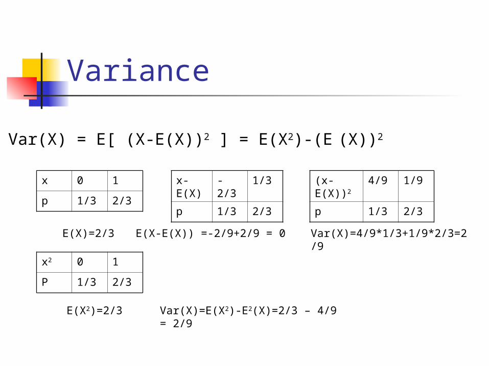
Variance

Var(X) = E[ (X-E(X))2 ] = E(X2)-(E (X))2

x 0 1

p 1/3 2/3

E(X)=2/3

x-E(X)

-2/3 1/3

p 1/3 2/3

E(X-E(X)) =-2/9+2/9 = 0

(x-E(X))2

4/9 1/9

p 1/3 2/3

Var(X)=4/9*1/3+1/9*2/3=2/9

x2 0 1

P 1/3 2/3

E(X2)=2/3 Var(X)=E(X2)-E2(X)=2/3 – 4/9 = 2/9

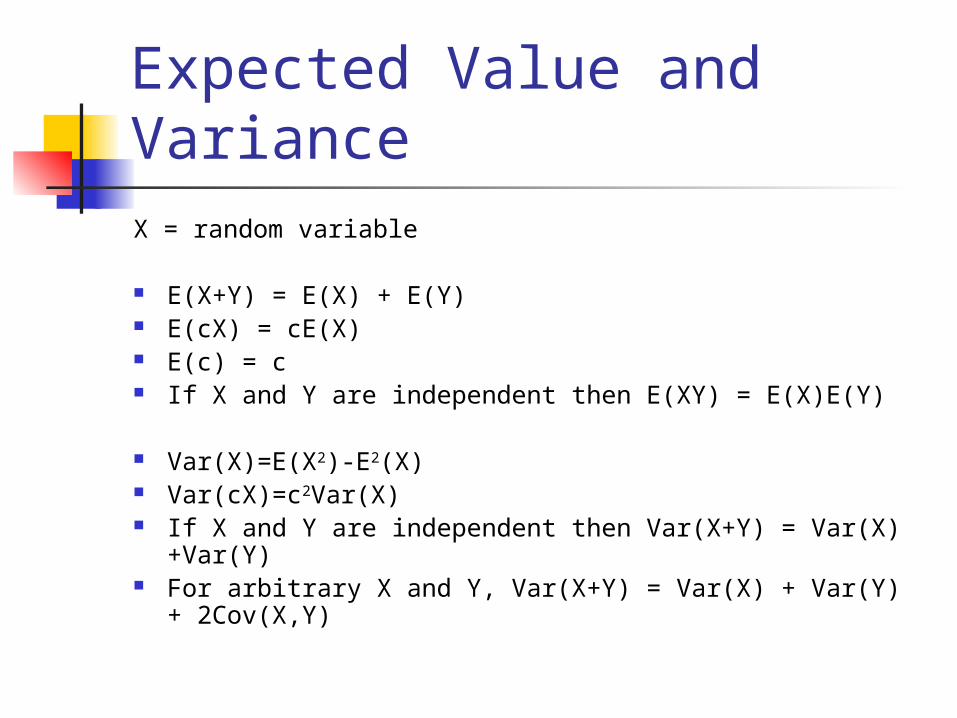
Expected Value and VarianceX = random variable

E(X+Y) = E(X) + E(Y) E(cX) = cE(X) E(c) = c If X and Y are independent then E(XY) = E(X)E(Y)

Var(X)=E(X2)-E2(X) Var(cX)=c2Var(X) If X and Y are independent then Var(X+Y) = Var(X)

+Var(Y) For arbitrary X and Y, Var(X+Y) = Var(X) + Var(Y) +

2Cov(X,Y)

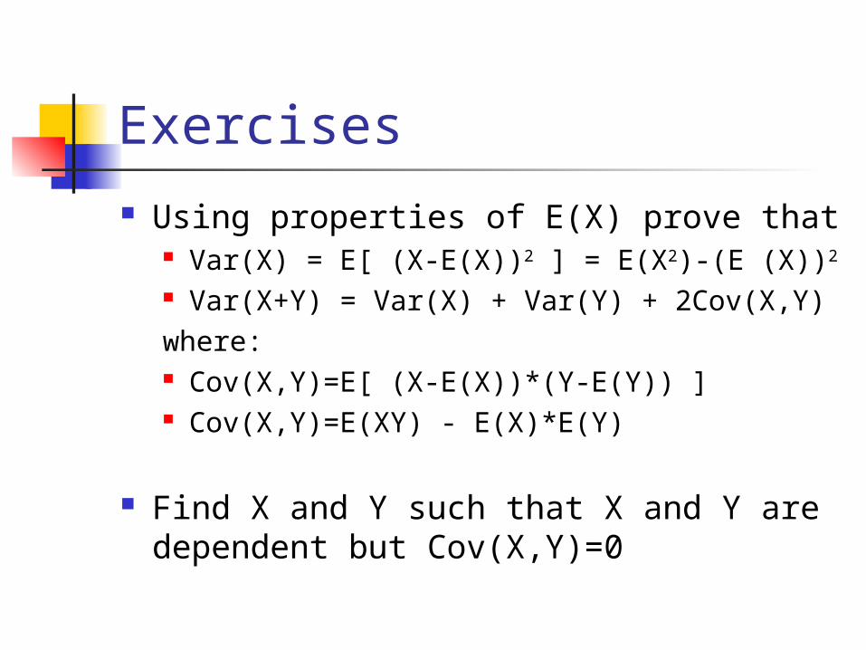
Exercises Using properties of E(X) prove that

Var(X) = E[ (X-E(X))2 ] = E(X2)-(E (X))2

Var(X+Y) = Var(X) + Var(Y) + 2Cov(X,Y) where: Cov(X,Y)=E[ (X-E(X))*(Y-E(Y)) ] Cov(X,Y)=E(XY) - E(X)*E(Y)

Find X and Y such that X and Y are dependent but Cov(X,Y)=0

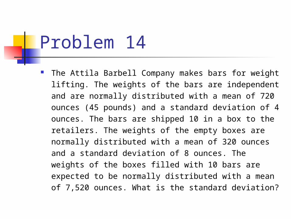
Problem 14 The Attila Barbell Company makes bars for weight

lifting. The weights of the bars are independent and are normally distributed with a mean of 720 ounces (45 pounds) and a standard deviation of 4 ounces. The bars are shipped 10 in a box to the retailers. The weights of the empty boxes are normally distributed with a mean of 320 ounces and a standard deviation of 8 ounces. The weights of the boxes filled with 10 bars are expected to be normally distributed with a mean of 7,520 ounces. What is the standard deviation?

Statistics

Part I: Sampling distribution

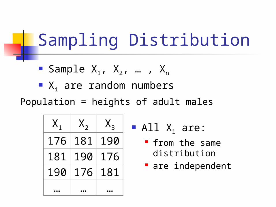
Sampling Distribution

Sample X1, X2, … , Xn

Xi are random numbersPopulation = heights of adult males

X1 X2 X3

176 181 190

181 190 176

190 176 181

… … …

All Xi are: from the same

distribution are independent

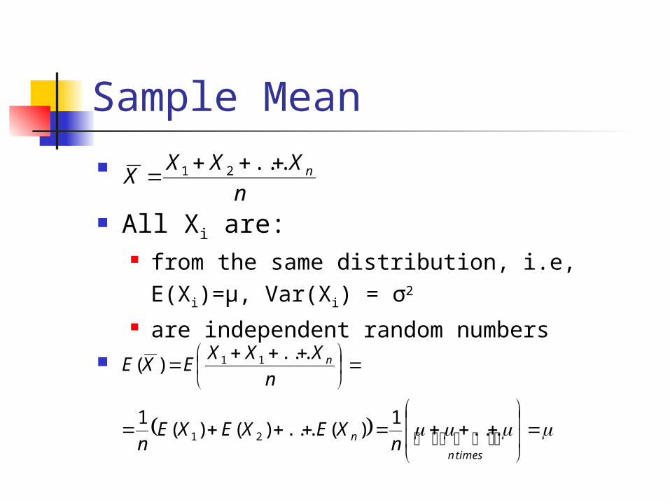
Sample Mean

All Xi are: from the same distribution, i.e,

E(Xi)=μ, Var(Xi) = σ2 are independent random numbers

n

XXXX n

...21

timesn

n

n

nXEXEXE

n

n

XXXEXE

...1

)(...)()(1

...)(

21

11

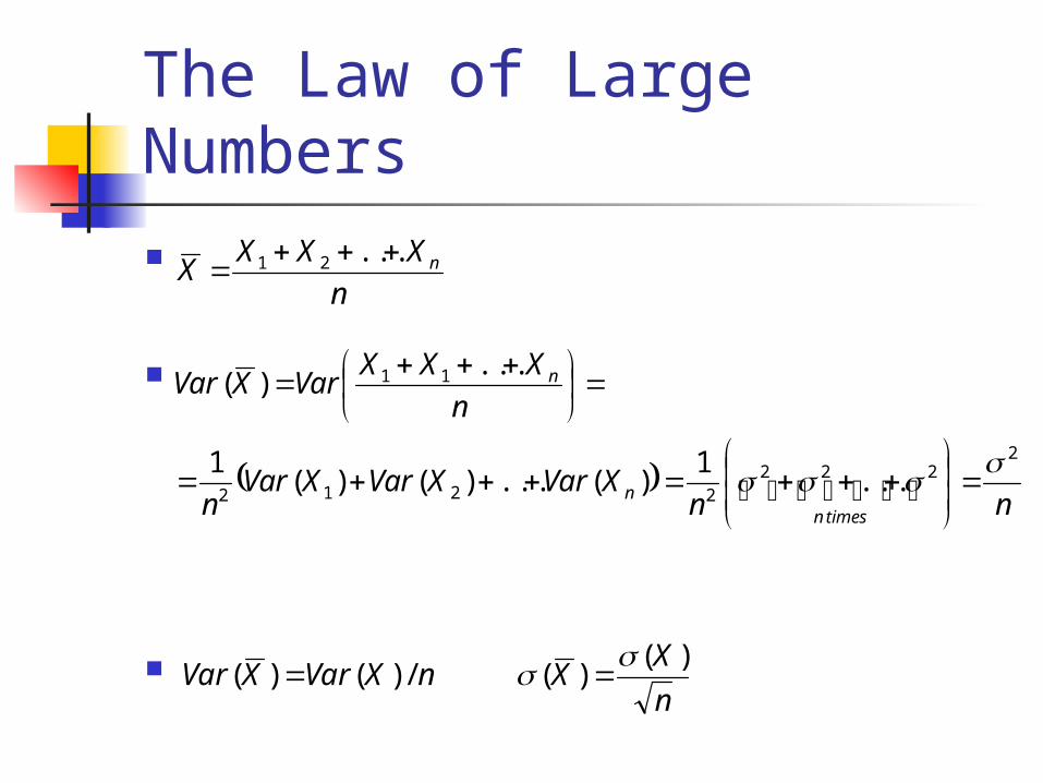
The Law of Large Numbers

n

XXnXVarXVar

)()(/)()(

n

XXXX n

...21

nn

XVarXVarXVarn

n

XXXVarXVar

timesnn

n

2222

2212

11

...1

)(...)()(1

...)(

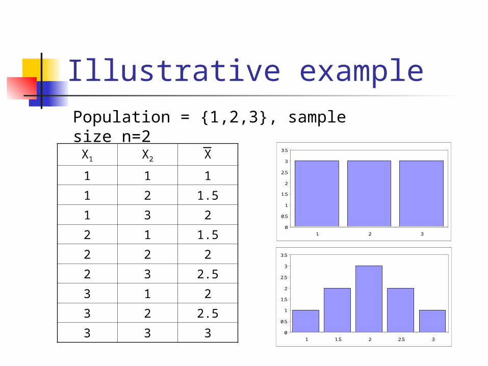
Illustrative example

X1 X2 X

1 1 1

1 2 1.5

1 3 2

2 1 1.5

2 2 2

2 3 2.5

3 1 2

3 2 2.5

3 3 3

Population = {1,2,3}, sample size n=2

0

0.5

1

1.5

2

2.5

3

3.5

1 2 3

0

0.5

1

1.5

2

2.5

3

3.5

1 1.5 2 2.5 3

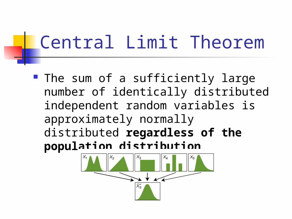
Central Limit Theorem

The sum of a sufficiently large number of identically distributed independent random variables is approximately normally distributed regardless of the population distribution

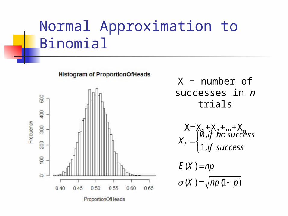
Normal Approximation to Binomial

X = number of successes in n trials

X=X1+X2+…+Xn

successif

successnoifX i ,1

,0

)1()(

)(

pnpX

npXE

Problem 18

There are two games involving flipping a coin. In the first game you win a prize if you can throw between 45% and 55% of heads. In the second game you win if you can throw more than 80% heads. For each game would you rather flip the coin 30 times or 300 times?

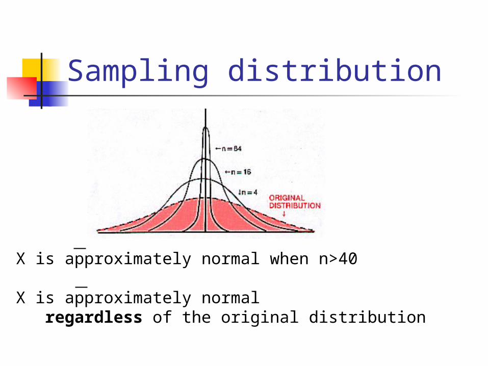
Sampling distribution

X is approximately normal when n>40

X is approximately normal regardless of the original distribution

Problem 15

The average outstanding bill for delinquent customer accounts for a national department store chain is $187.50 with a standard deviation of $54.50. In a simple random sample of 50 delinquent accounts, what is the probability that the mean outstanding bill is over $200?

Problem 16

The average number of daily emergency room admissions at a hospital is 85 with standard deviation of 37. In a simple random sample of 30 days, what is the probability that the mean number of daily emergency admissions is between 75 and 95?

Problem 17

A summer resort rents rowboats to customers but does not allow more than four people to a boat. Each boat is designed to hold no more than 800 pounds. Suppose the distribution of adult males who rent boats, including their clothes and gear, is normal with a mean of 190 pounds and standard deviation of 10 pounds. If the weights of individual passengers are independent, what is the probability that a group of four adult male passengers will exceed the acceptable weight limit of 800 pounds?

Statistics

Part II: Hypothesis testing

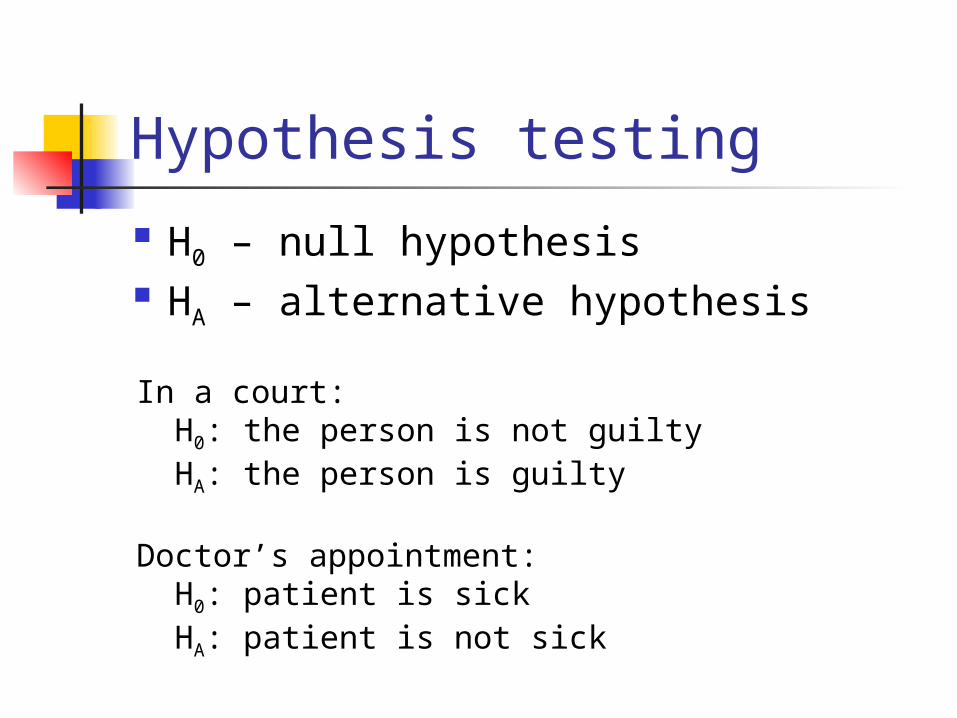
Hypothesis testing

H0 – null hypothesis HA – alternative hypothesis

In a court: H0: the person is not guilty HA: the person is guilty

Doctor’s appointment: H0: patient is sick HA: patient is not sick

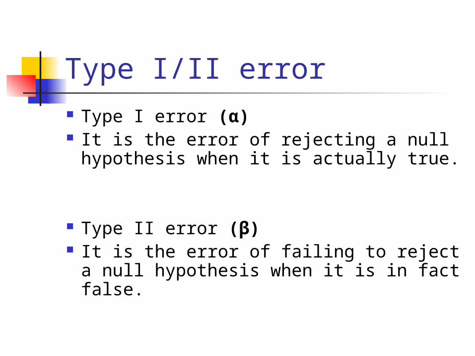
Type I/II error Type I error (α) It is the error of rejecting a null

hypothesis when it is actually true.

Type II error (β) It is the error of failing to reject a null

hypothesis when it is in fact false.

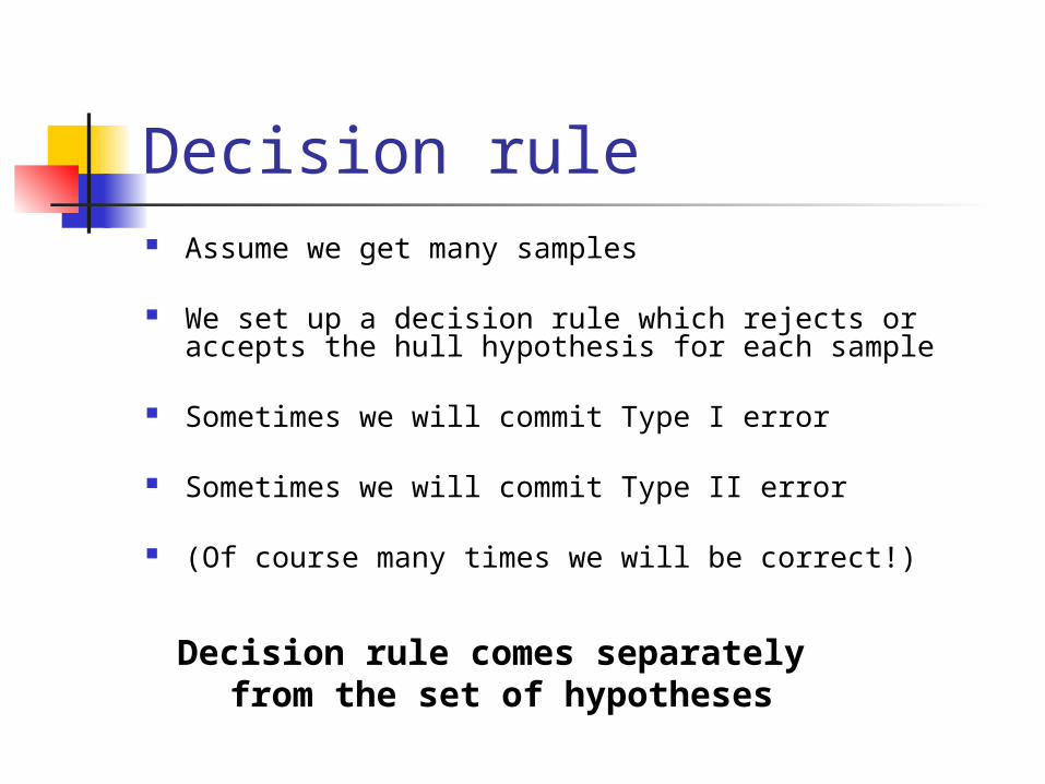
Decision rule Assume we get many samples

We set up a decision rule which rejects or accepts the hull hypothesis for each sample

Sometimes we will commit Type I error

Sometimes we will commit Type II error

(Of course many times we will be correct!)

Decision rule comes separately from the set of hypotheses

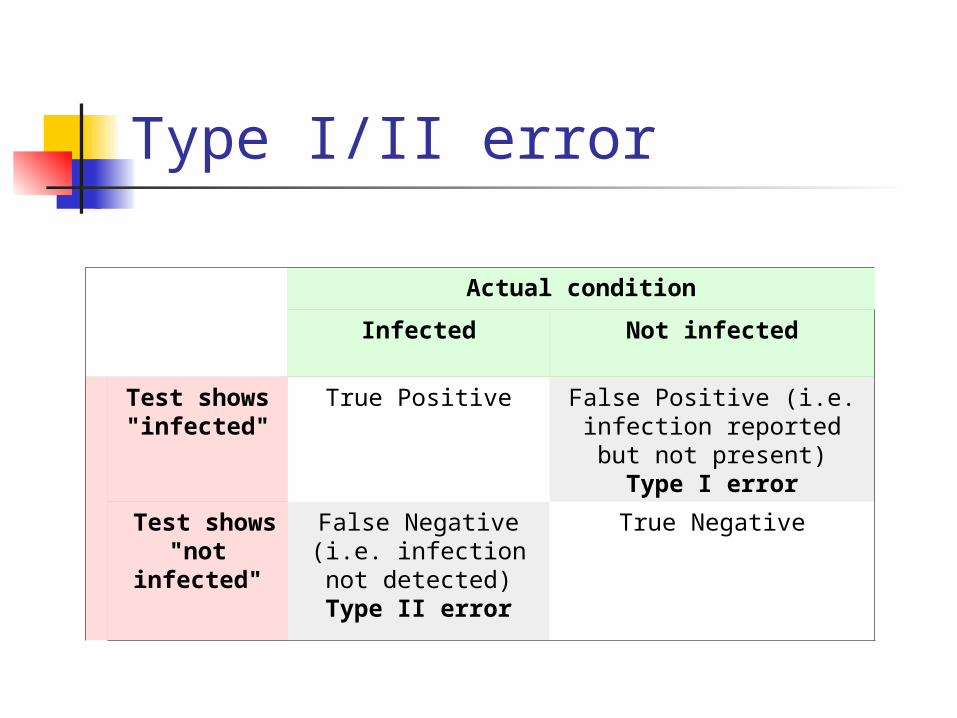
Type I/II error

 Actual condition

Infected Not infected

Test shows "infected"

True Positive False Positive (i.e. infection reported but not present)

Type I error

 Test shows "not infected"

False Negative (i.e. infection not detected)

Type II error

True Negative

Problem 19

A patient claims that he consumes only 2000 calories per day, but a dietician suspects that the actual figure is higher. The dietician plans to check his food intake for 30 days and will reject the patient's claim if the 30-day-mean is more than 2100 calories. If the standard deviation (in calories per day) is 350, what is the probability that the dietician will mistakenly reject a patient's true claim?

Problem 20 City planners wish to test the claim that shoppers

park for an average of only 47 minutes in the downtown area. The planners have decided to tabulate parking durations for 225 shoppers and to reject the claim if the sample mean exceeds 50 minutes. If the claim is wrong and the true mean is 51 minutes, what is the probability that the random sample will lead to a mistaken failure to reject the claim? Assume that the standard deviation in parking durations is 27 minutes.

P-value P-value is the probability of obtaining a

result at least as extreme as the one that was actually observed, given that the null hypothesis is true.

Если бы то, что мы предполагаем в нулевой гипотезе было верно, то какова была бы вероятность видеть то, что мы видим в выборке (это, или еще «хуже»)

Hypothesis testing

P-value is a function of sample α is a function of decision rule

Reject H0 if p-value< α Small p-value indicates that you see

something very unusual if H0 were true

Problem 21

A service station advertises that its mechanics can change a muffler in only 15 minutes. A consumers group doubts this claim and runs a hypothesis test using 49 cars needing new mufflers. In this sample the mean changing time is 16.25 minutes with a standard deviation of 3.5 minutes. Is this a strong evidence against the 15 minute claim?

Estimators An estimator is a function of the

observable sample data that is used to estimate an unknown population parameter

is an estimator for μ s is an estimator for σ is an estimator for p

X

p

Unbiased effective estimators

Let be the unknown parameter Let be an estimator

is unbiased if is effective if

n

)ˆ( nE

0)ˆ(lim n

nVar

n

n

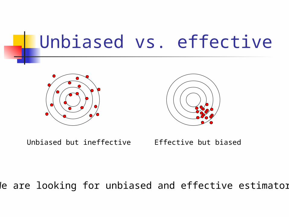
Unbiased vs. effective

Unbiased but ineffective Effective but biased

We are looking for unbiased and effective estimators

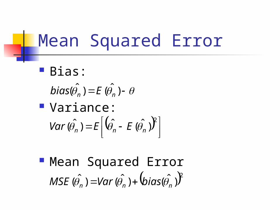
Mean Squared Error

Bias:

Variance:

Mean Squared Error

)ˆ()ˆ( nn Ebias

2)ˆ(ˆ)ˆ( nnn EEVar

2)ˆ()ˆ()ˆ( nnn biasVarMSE

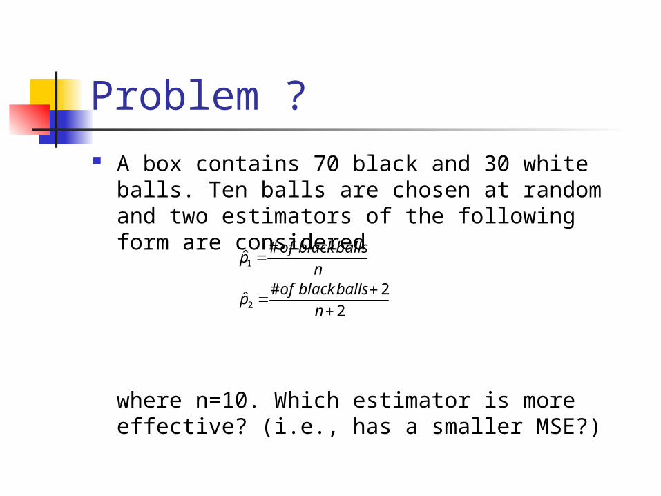
Problem ? A box contains 70 black and 30 white balls.

Ten balls are chosen at random and two estimators of the following form are considered

where n=10. Which estimator is more effective? (i.e., has a smaller MSE?)

2

2#ˆ

#ˆ

2

1

n

ballsblackofp

n

ballsblackofp

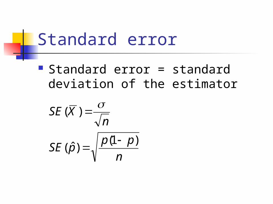
Standard error

Standard error = standard deviation of the estimator

n

pppSE

nXSE

)1()ˆ(

)(

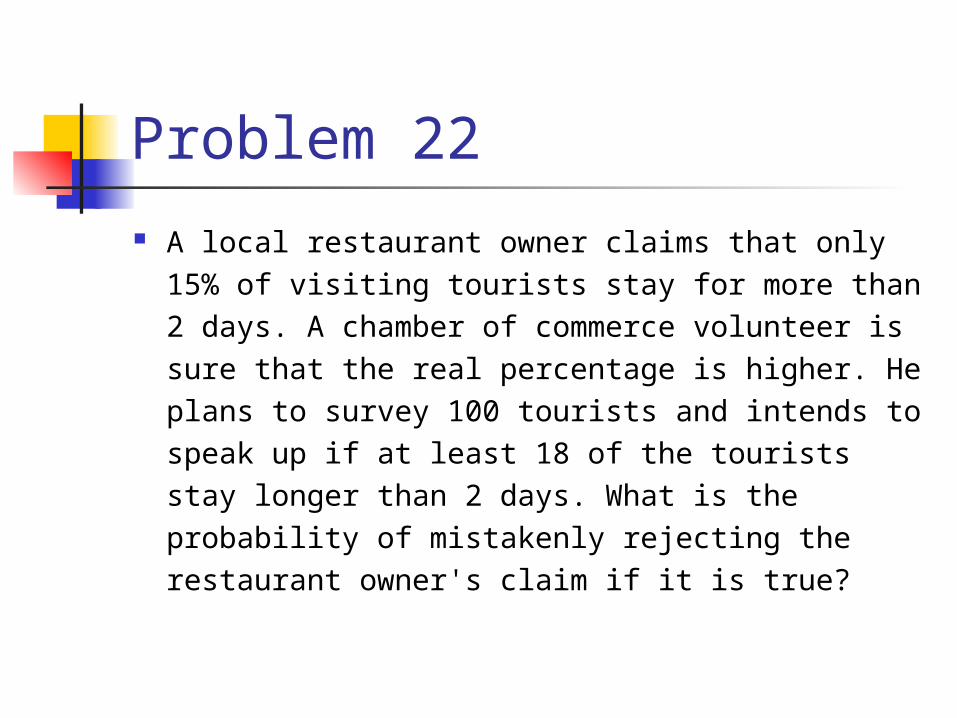
Problem 22

A local restaurant owner claims that only 15% of visiting tourists stay for more than 2 days. A chamber of commerce volunteer is sure that the real percentage is higher. He plans to survey 100 tourists and intends to speak up if at least 18 of the tourists stay longer than 2 days. What is the probability of mistakenly rejecting the restaurant owner's claim if it is true?

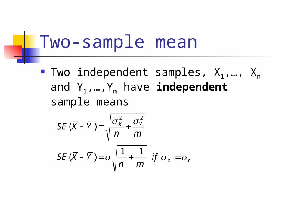
Two-sample mean

Two independent samples, X1,…, Xn and Y1,…,Ym have independent sample means

YX

YX

ifmn

YXSE

mnYXSE

11)(

)(22

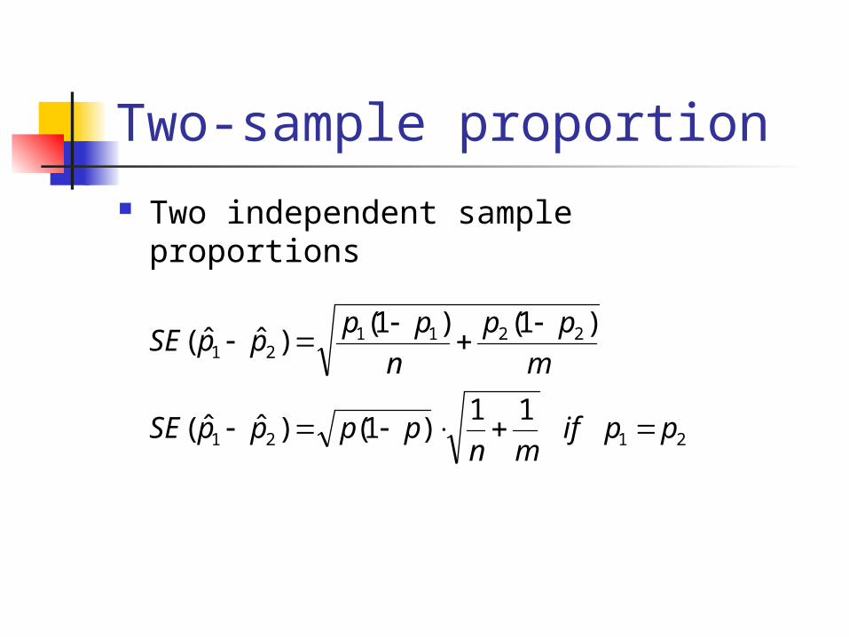
Two-sample proportion Two independent sample proportions

2121

221121

11)1()ˆˆ(

)1()1()ˆˆ(

ppifmn

ppppSE

m

pp

n

ppppSE

Problem 23 A historian believes that the average height of

soldiers in World War II was greater than that of soldiers in World War I. She examines a random sample of records of 100 men in each war and notes standard deviations of 2.5 and 2.3 inches in World War I and World War II, respectively. If the average height from the sample of World War II soldiers is 1 inch greater than that from the sample of World War I soldiers, what conclusion is justified from a two-sample hypothesis test where H0: μ1 = μ2 vs. HA: μ1< μ2?

Confidence intervals Hypothesis testing: A coffee machine is supposed to

deliver 8 ounces of coffee in a cup, but in my sample of 10 cups I get only 7.5 ounces. Is this ok?

Confidence intervals: My sample of 10 cups of coffee contains on average 7.5 ounces of liquid. What is the likely estimate for the mean amount of coffee per cup?

Hypothesis testing and construction of confidence intervals are mutually inverse problems

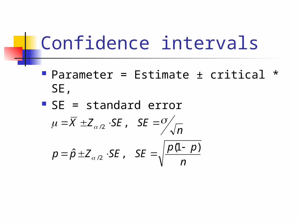
Confidence intervals

Parameter = Estimate ± critical * SE, SE = standard error

n

ppSESEZpp

nSESEZX

)1(,ˆ

,

2/

2/

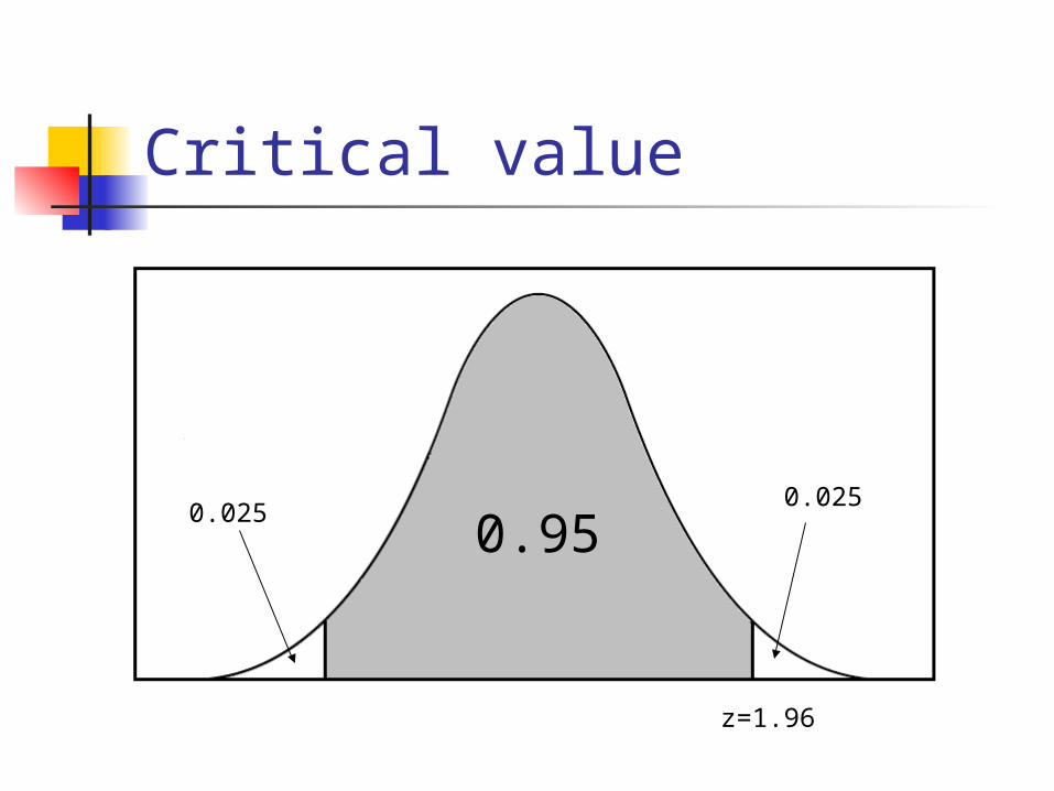
Critical value

0.950.025

0.025

z=1.96

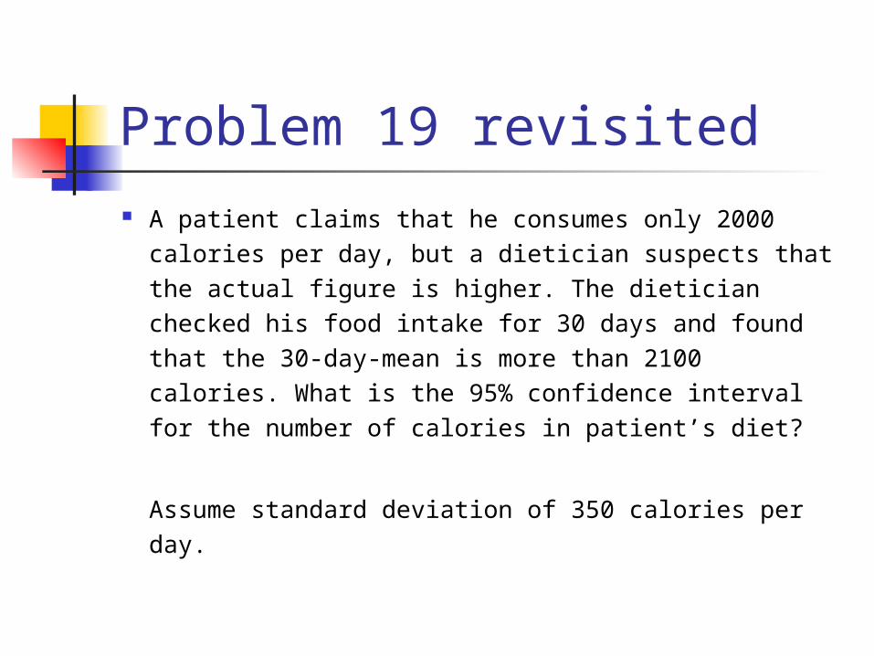
Problem 19 revisited

A patient claims that he consumes only 2000 calories per day, but a dietician suspects that the actual figure is higher. The dietician checked his food intake for 30 days and found that the 30-day-mean is more than 2100 calories. What is the 95% confidence interval for the number of calories in patient’s diet?

Assume standard deviation of 350 calories per day.

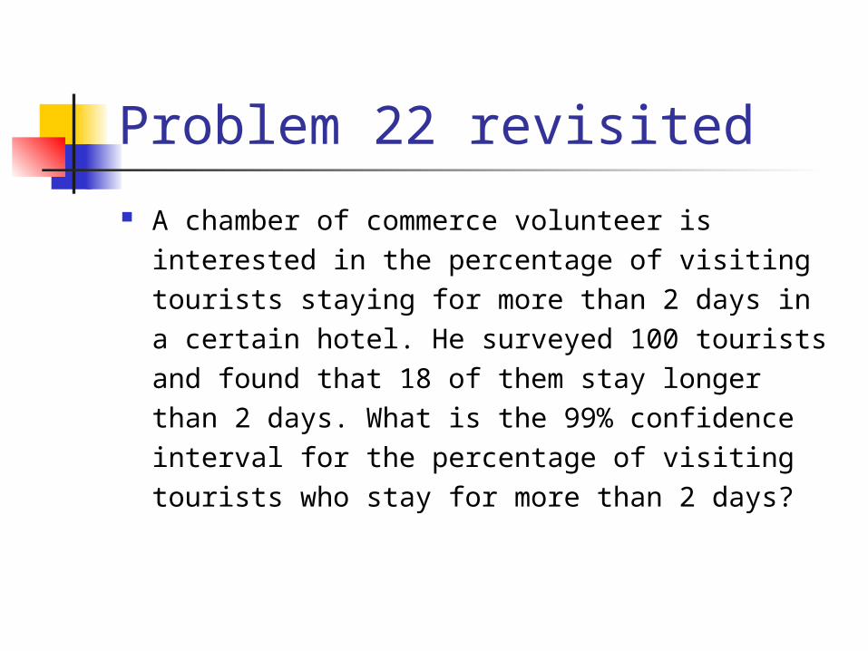
Problem 22 revisited

A chamber of commerce volunteer is interested in the percentage of visiting tourists staying for more than 2 days in a certain hotel. He surveyed 100 tourists and found that 18 of them stay longer than 2 days. What is the 99% confidence interval for the percentage of visiting tourists who stay for more than 2 days?

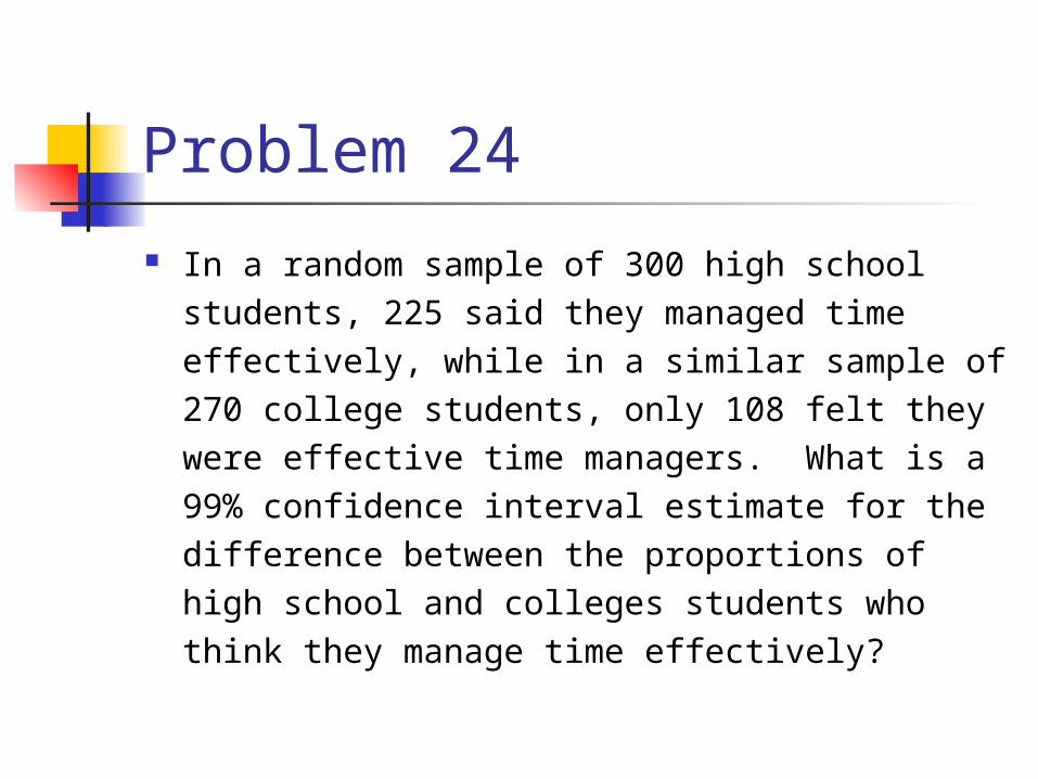
Problem 24

In a random sample of 300 high school students, 225 said they managed time effectively, while in a similar sample of 270 college students, only 108 felt they were effective time managers. What is a 99% confidence interval estimate for the difference between the proportions of high school and colleges students who think they manage time effectively?

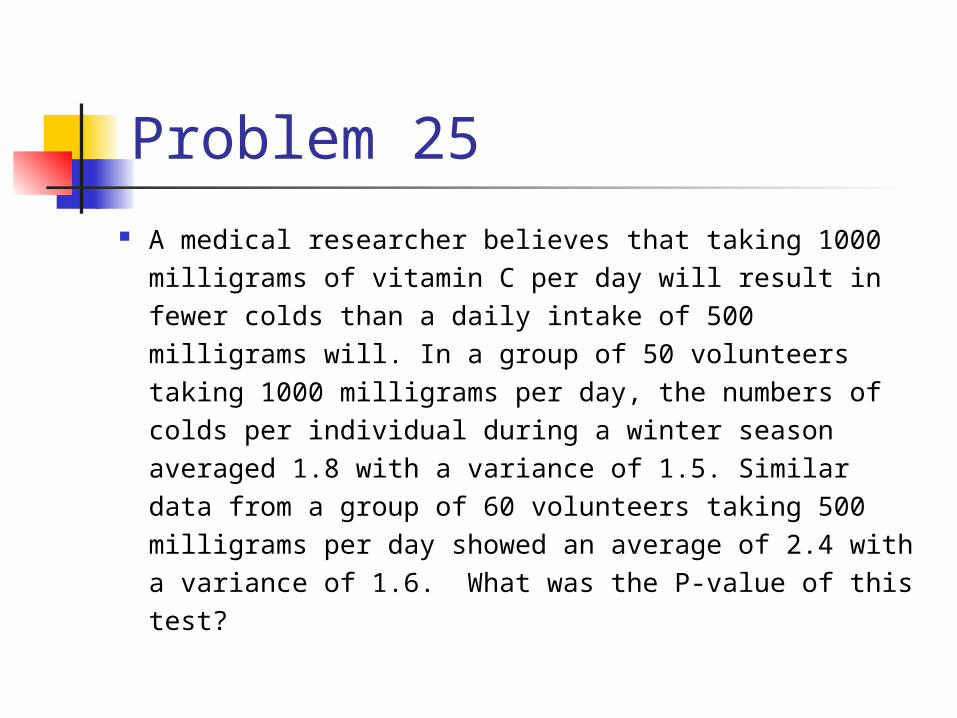
Problem 25

A medical researcher believes that taking 1000 milligrams of vitamin C per day will result in fewer colds than a daily intake of 500 milligrams will. In a group of 50 volunteers taking 1000 milligrams per day, the numbers of colds per individual during a winter season averaged 1.8 with a variance of 1.5. Similar data from a group of 60 volunteers taking 500 milligrams per day showed an average of 2.4 with a variance of 1.6. What was the P-value of this test?

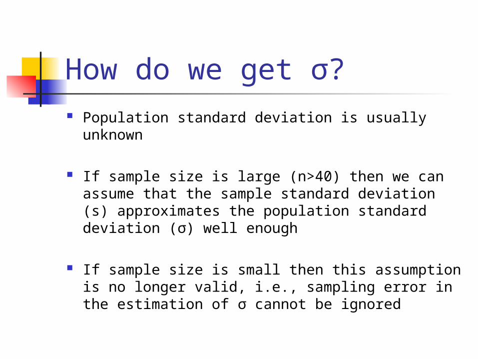
How do we get σ? Population standard deviation is usually

unknown

If sample size is large (n>40) then we can assume that the sample standard deviation (s) approximates the population standard deviation (σ) well enough

If sample size is small then this assumption is no longer valid, i.e., sampling error in the estimation of σ cannot be ignored

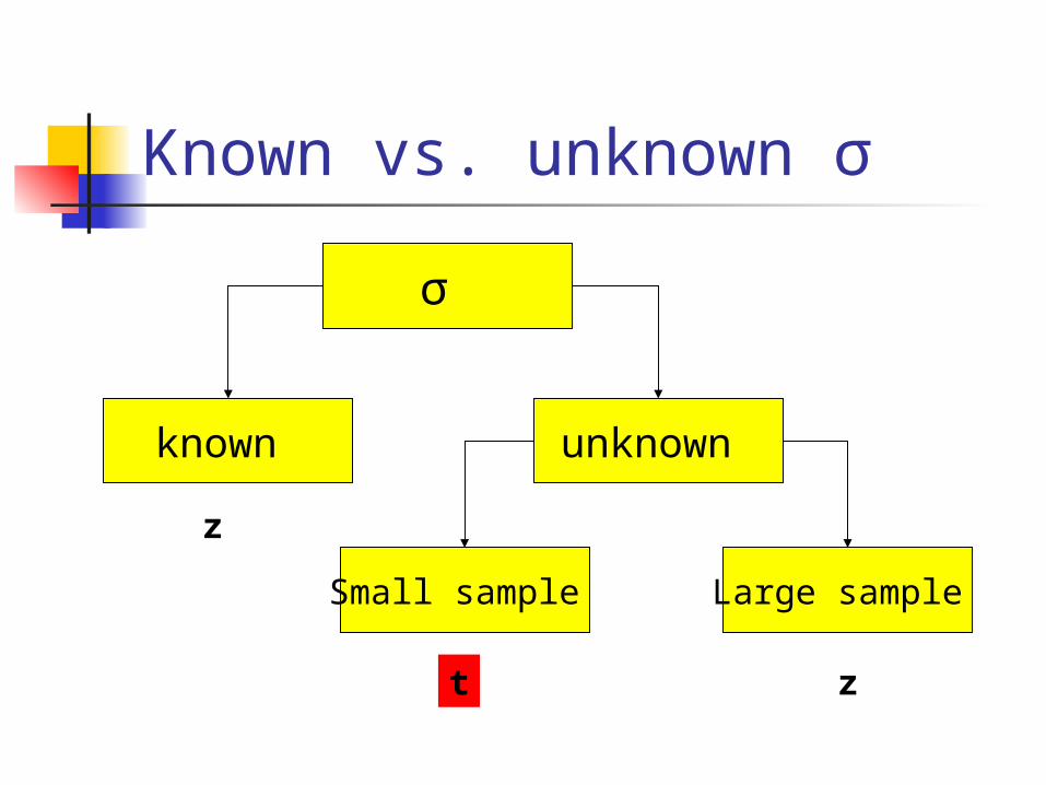
Known vs. unknown σ

σ

known unknown

Small sample Large sample

z

t z

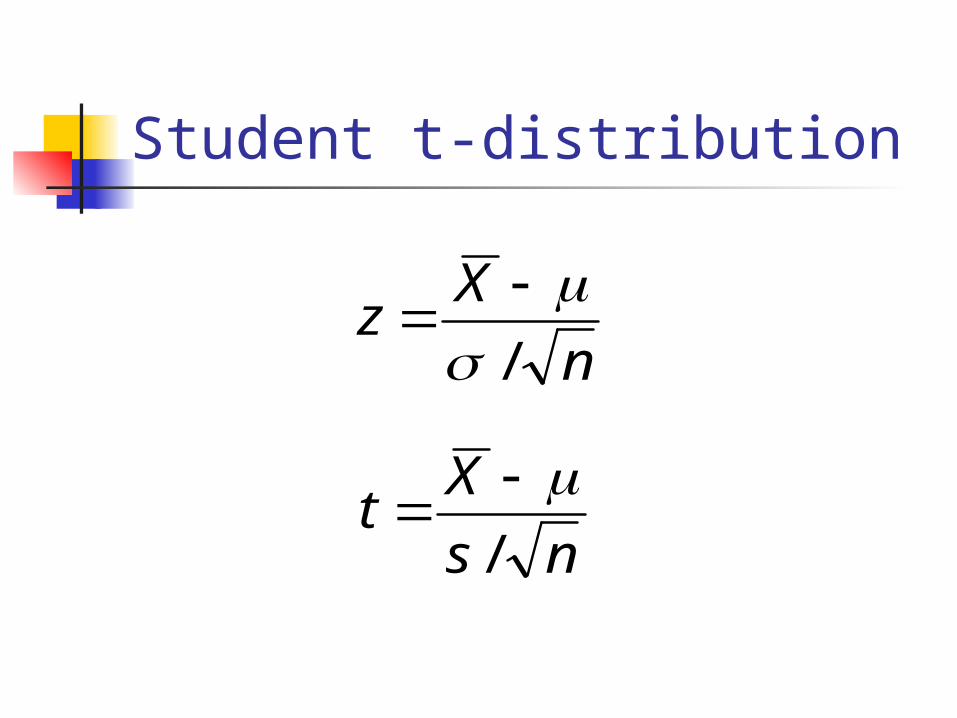
Student t-distribution

n

Xz

/

ns

Xt

/

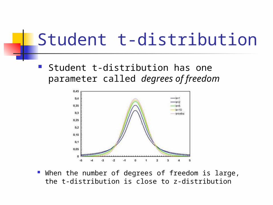
Student t-distribution Student t-distribution has one parameter

called degrees of freedom

When the number of degrees of freedom is large, the t-distribution is close to z-distribution

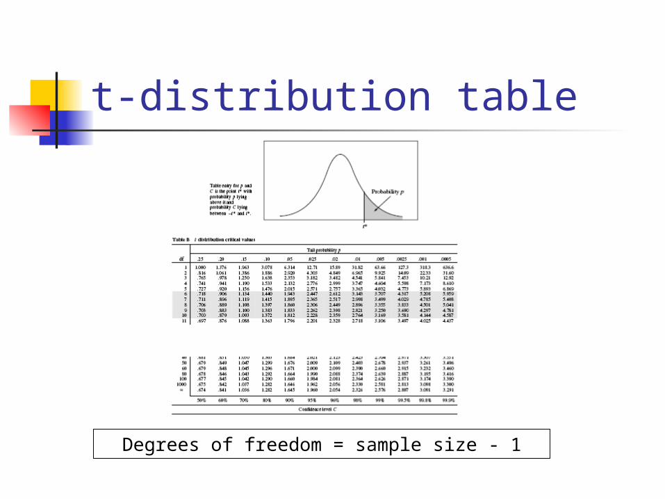
t-distribution table

Degrees of freedom = sample size - 1

Problem 26

An article ("Undergraduate Marijuana use and Anger" by Sue Stoner) in a 1988 issue of the Journal of Psychology (Vol. 122, p. 33) reported that in a sample of 17 marijuana users the mean and standard deviation on an anger expression scale were 42.72 and 6.05, respectively. Test whether this result is significantly greater than the established mean of 41.6 for nonusers. What assumptions are necessary for the above test to be valid?

T-test assumptions Random sampling (like in z-test)

Normal population (unlike z-test, where sample mean is automatically normal regardless of the population when sample size is large)

Degrees of freedom = number of independent observations (actually, residuals)

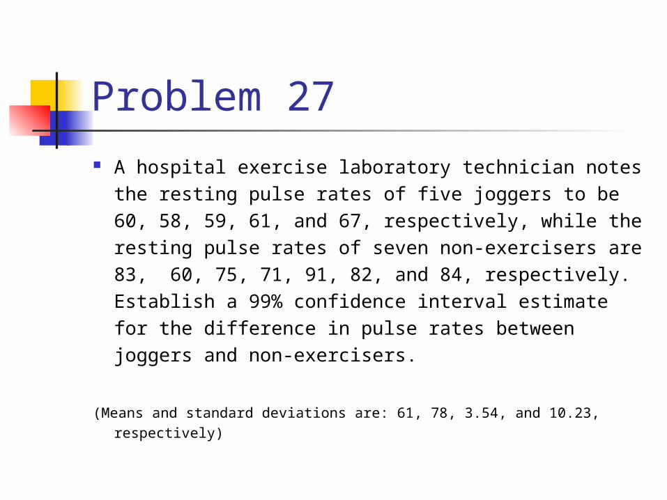
Problem 27

A hospital exercise laboratory technician notes the resting pulse rates of five joggers to be 60, 58, 59, 61, and 67, respectively, while the resting pulse rates of seven non-exercisers are 83, 60, 75, 71, 91, 82, and 84, respectively. Establish a 99% confidence interval estimate for the difference in pulse rates between joggers and non-exercisers.

(Means and standard deviations are: 61, 78, 3.54, and 10.23, respectively)

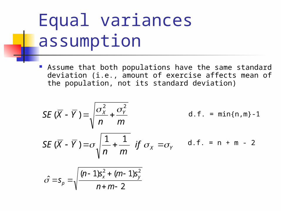
Equal variances assumption Assume that both populations have the same

standard deviation (i.e., amount of exercise affects mean of the population, not its standard deviation)

YX

YX

ifmn

YXSE

mnYXSE

11)(

)(22

d.f. = min{n,m}-1

d.f. = n + m - 2

2

)1()1(ˆ

22

mn

smsns yx

p

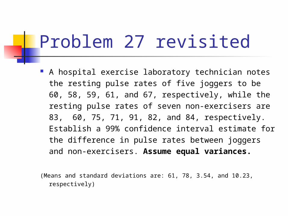
Problem 27 revisited A hospital exercise laboratory technician notes the

resting pulse rates of five joggers to be 60, 58, 59, 61, and 67, respectively, while the resting pulse rates of seven non-exercisers are 83, 60, 75, 71, 91, 82, and 84, respectively. Establish a 99% confidence interval estimate for the difference in pulse rates between joggers and non-exercisers. Assume equal variances.

(Means and standard deviations are: 61, 78, 3.54, and 10.23, respectively)

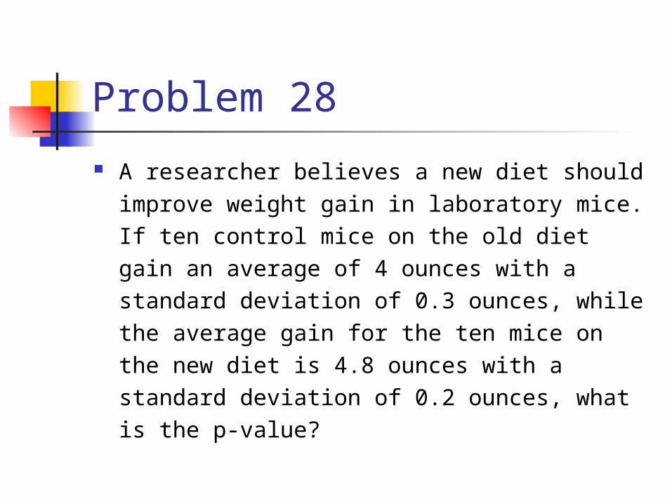
Problem 28

A researcher believes a new diet should improve weight gain in laboratory mice. If ten control mice on the old diet gain an average of 4 ounces with a standard deviation of 0.3 ounces, while the average gain for the ten mice on the new diet is 4.8 ounces with a standard deviation of 0.2 ounces, what is the p-value?

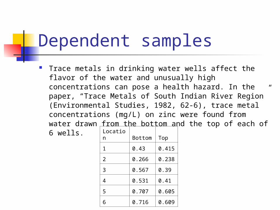
Dependent samples Trace metals in drinking water wells affect the flavor of

the water and unusually high concentrations can pose a health hazard. In the paper, “Trace Metals of South Indian River Region” (Environmental Studies, 1982, 62-6), trace metal concentrations (mg/L) on zinc were found from water drawn from the bottom and the top of each of 6 wells.

Location Bottom Top

1 0.43 0.415

2 0.266 0.238

3 0.567 0.39

4 0.531 0.41

5 0.707 0.605

6 0.716 0.609

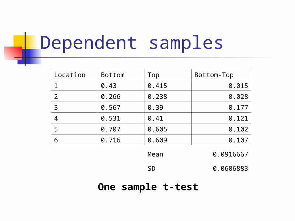
Dependent samples

Location Bottom Top Bottom-Top

1 0.43 0.415 0.015

2 0.266 0.238 0.028

3 0.567 0.39 0.177

4 0.531 0.41 0.121

5 0.707 0.605 0.102

6 0.716 0.609 0.107

Mean 0.0916667

SD 0.0606883

One sample t-test

FAQs Do I have to divide by square root of n?

Yes, if you are looking for P(X>100) No, if you are looking for P(X>100)

Do I have to divide by square root of n in one-proportion or two-proportion tests? No. If you use Standard Error, it already contains the

square root of n

When I compute standard deviation from the sample, do I have to divide it by square root of n? Yes, if your calculations involve sample mean.

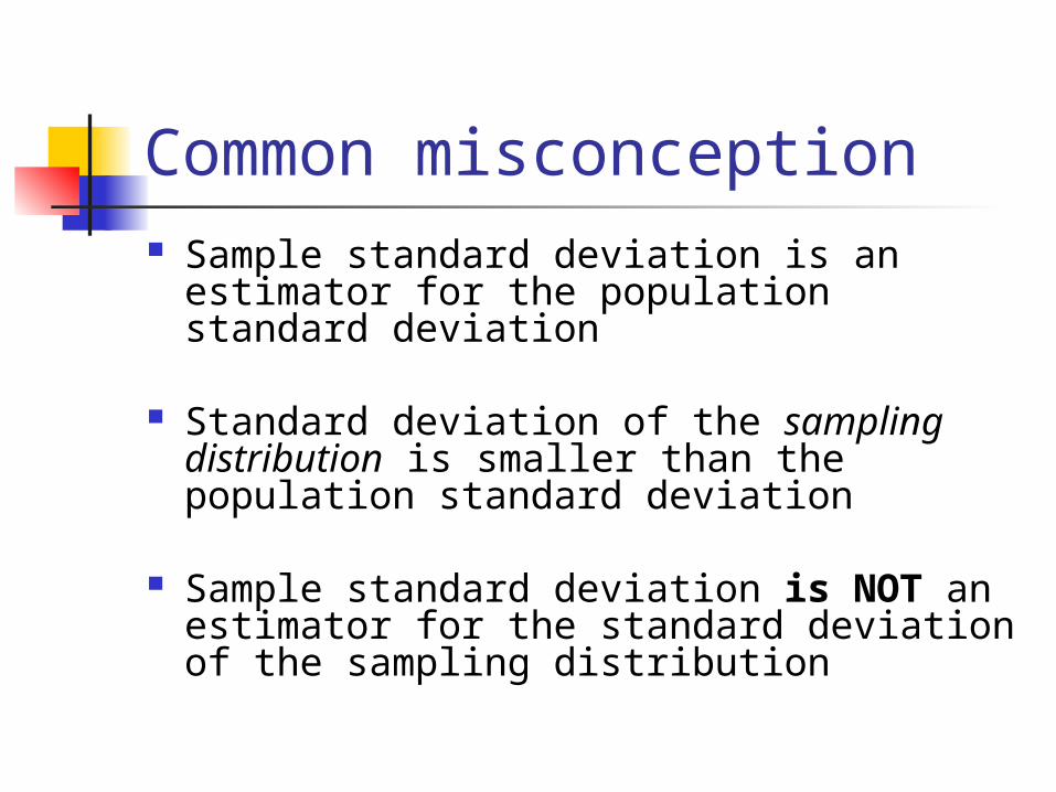
Common misconception Sample standard deviation is an

estimator for the population standard deviation

Standard deviation of the sampling distribution is smaller than the population standard deviation

Sample standard deviation is NOT an estimator for the standard deviation of the sampling distribution

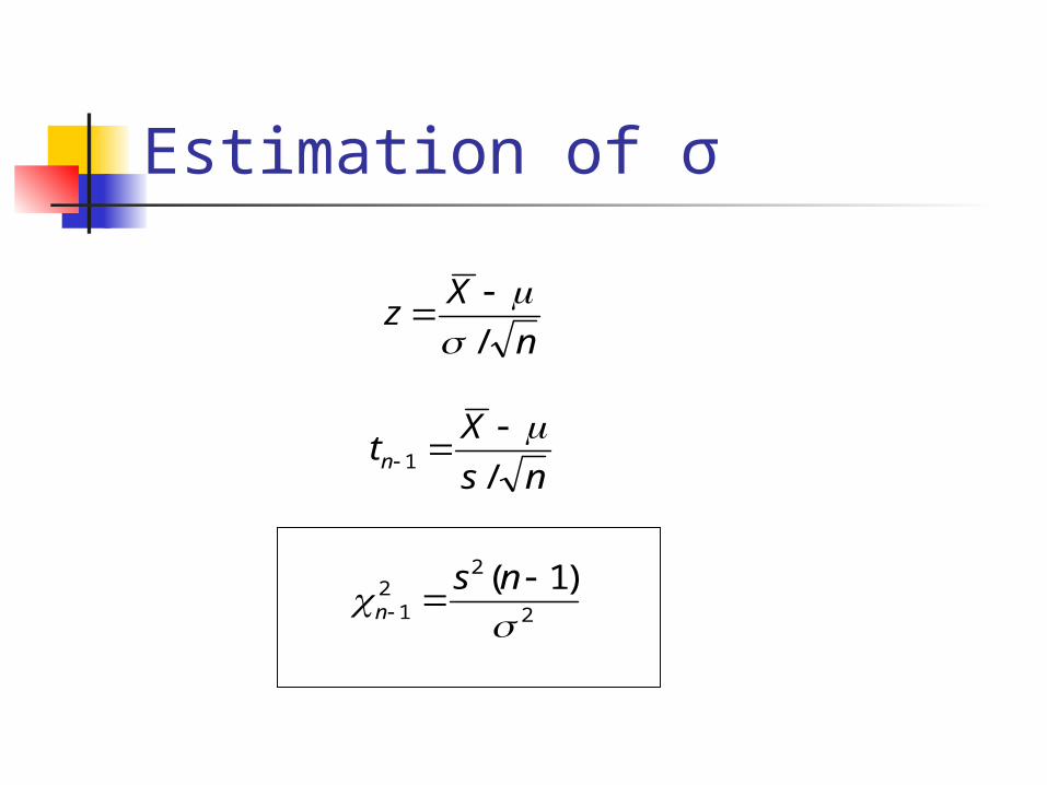
Estimation of σ

n

Xz

/

ns

Xtn

/1

2

22

1

)1(

ns

n

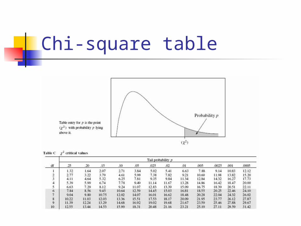
Chi-square table

Problem 29

A supplier of 100 ohm/cm silicon wafers claims that his fabrication process can produce wafers with sufficient consistency so that the standard deviation of resistance for the lot does not exceed 10 ohm/cm. A sample of 10 wafers taken from the lot has a standard deviation of 13.97 ohm/cm. Is the suppliers claim reasonable?

Problem 30

A container of oil is supposed to contain 1000 ml of oil. We want to be sure that the standard deviation of the oil container is less than 20 ml. We randomly select 10 cans of oil with a mean of 997 ml and a standard deviation of 32 ml. Using these sample construct a 95% confidence interval for the true value of sigma. Does the confidence interval suggest that the variation in oil containers is at an acceptable level?

Estimation of sample size What is a minimum sample size needed

to estimate the population mean within 2 units?

What is a minimum sample size needed to estimate the population proportion within 2 percent units?

Problem 31

An electrical firm which manufactures a certain type of bulb wants to estimate its mean life. Assuming that the life of the light bulb is normally distributed and that the standard deviation is known to be 40 hours, how many bulbs should be tested so that we can be 90 percent confident that the estimate of the mean will not differ from the true mean life by more than 10 hours?

Problem 32

A quality control engineer wants to estimate the fraction of defective bulbs in a large lot of light bulbs. From past experience, he feels that the actual fraction of defective bulbs should be somewhere around 0.2 . How large a sample should be taken if he wants to estimate the true fraction within .02 using a 95% confidence interval?

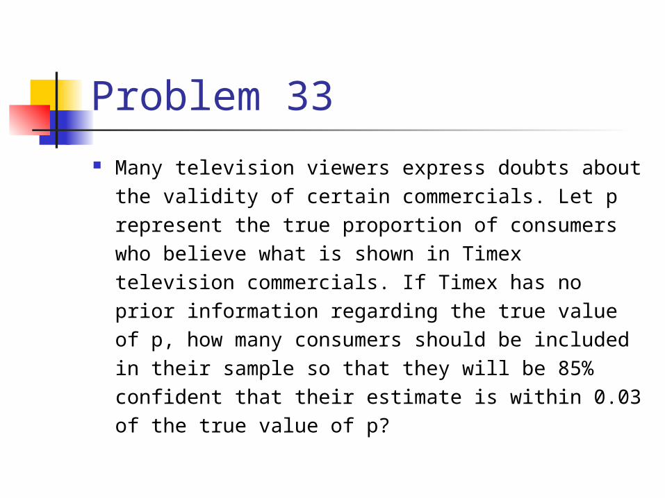
Problem 33

Many television viewers express doubts about the validity of certain commercials. Let p represent the true proportion of consumers who believe what is shown in Timex television commercials. If Timex has no prior information regarding the true value of p, how many consumers should be included in their sample so that they will be 85% confident that their estimate is within 0.03 of the true value of p?

Statistics

Part III: Contingency tables

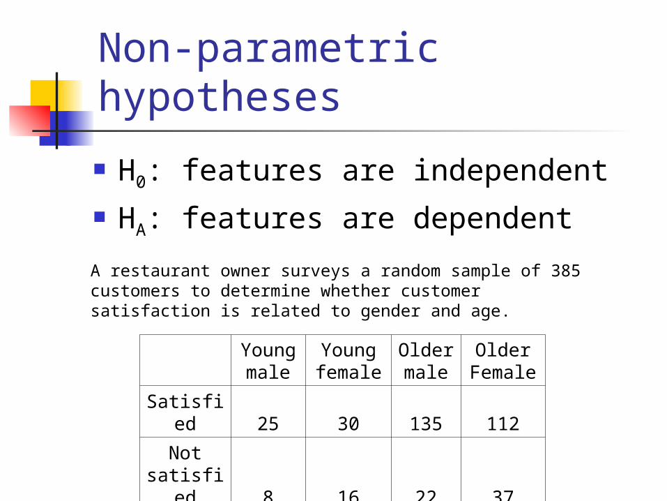
Non-parametric hypotheses

H0: features are independent HA: features are dependent

 Young male

Young female

Older male

Older Female

Satisfied 25 30 135 112

Not satisfied 8 16 22 37

A restaurant owner surveys a random sample of 385 customers to determine whether customer satisfaction is related to gender and age.

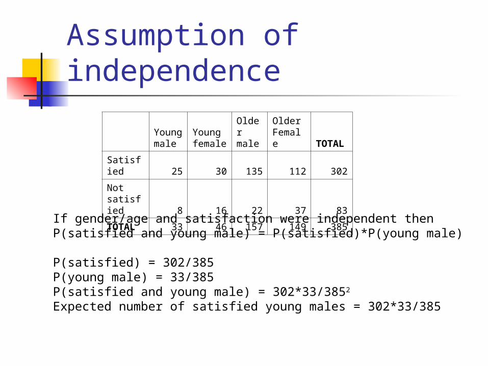
Assumption of independence

 Young male

Young female

Older male

Older Female TOTAL

Satisfied 25 30 135 112 302

Not satisfied 8 16 22 37 83

TOTAL 33 46 157 149 385

If gender/age and satisfaction were independent thenP(satisfied and young male) = P(satisfied)*P(young male)

P(satisfied) = 302/385P(young male) = 33/385P(satisfied and young male) = 302*33/3852

Expected number of satisfied young males = 302*33/385

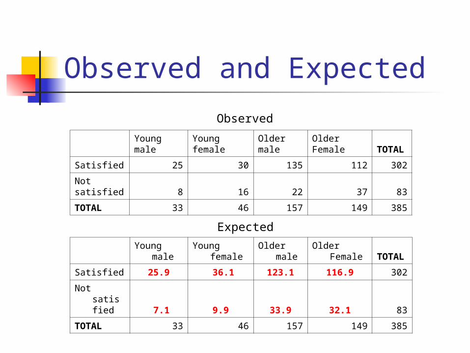
Observed and Expected

 Young

maleYoung

femaleOlder

maleOlder

Female TOTAL

Satisfied 25.9  36.1 123.1 116.9 302

Not satisfied  7.1 9.9 33.9 32.1 83

TOTAL 33 46 157 149 385

 Young male

Young female

Older male

Older Female TOTAL

Satisfied 25 30 135 112 302

Not satisfied 8 16 22 37 83

TOTAL 33 46 157 149 385

Observed

Expected

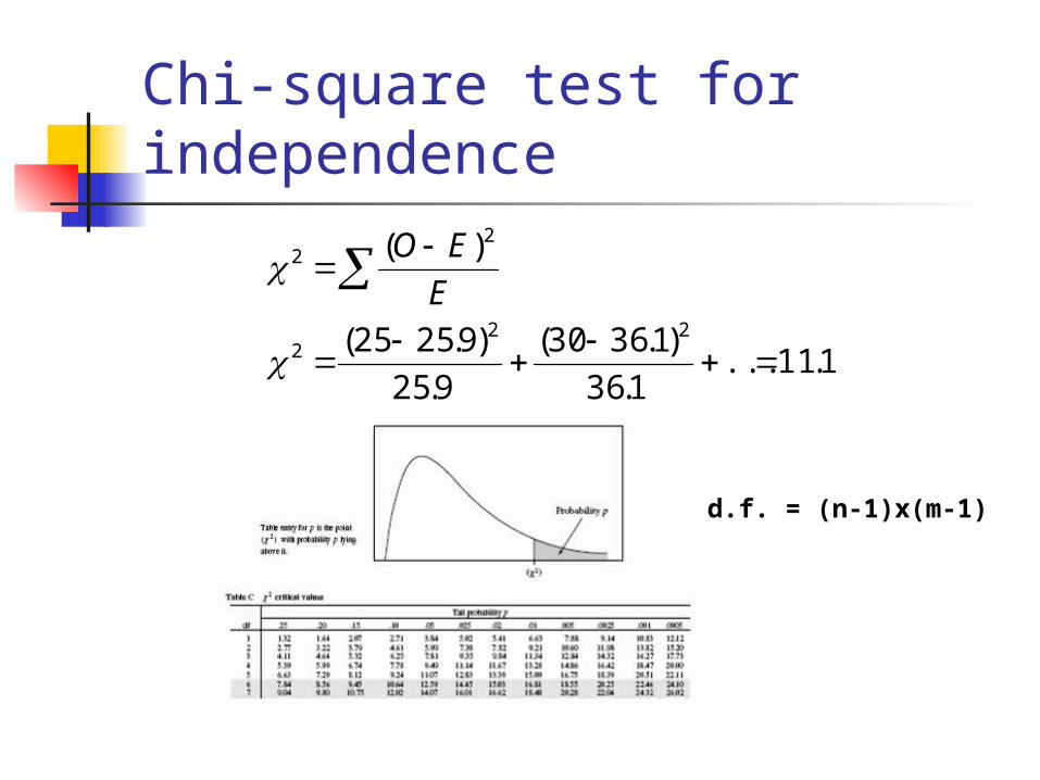
Chi-square test for independence

1.11...1.36

)1.3630(

9.25

)9.2525(

)(

222

22

E

EO

d.f. = (n-1)x(m-1)

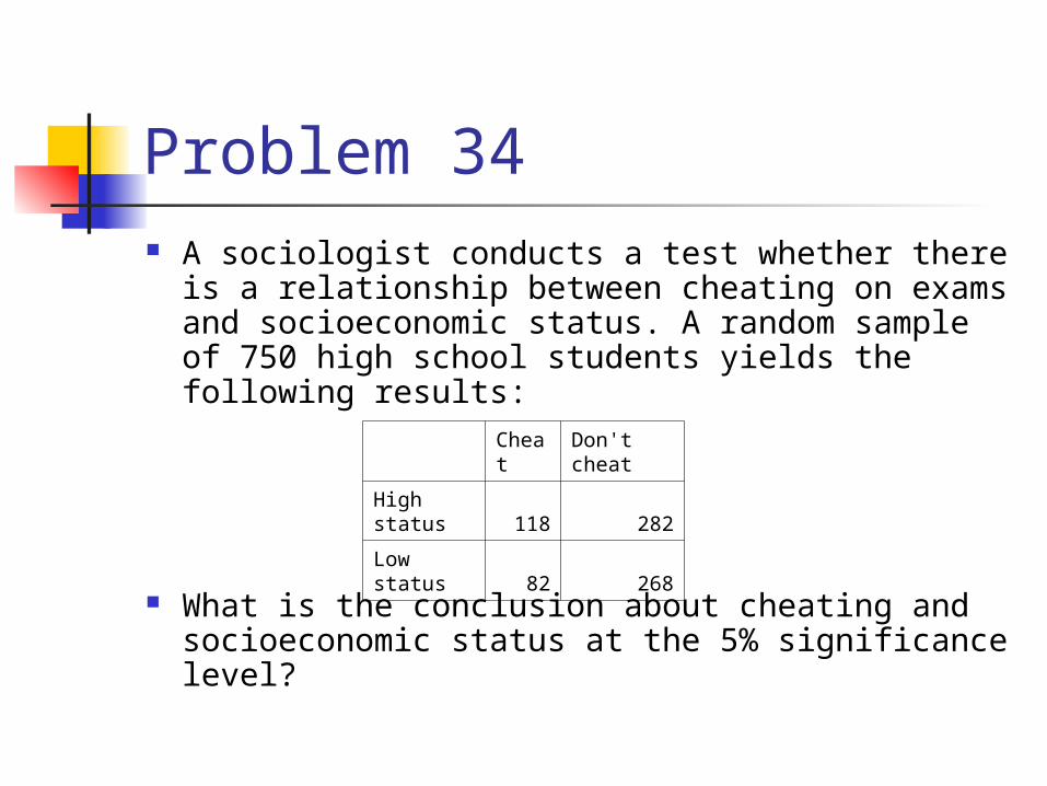
Problem 34 A sociologist conducts a test whether there is a

relationship between cheating on exams and socioeconomic status. A random sample of 750 high school students yields the following results:

What is the conclusion about cheating and socioeconomic status at the 5% significance level?

  CheatDon't cheat

High status 118 282

Low status 82 268

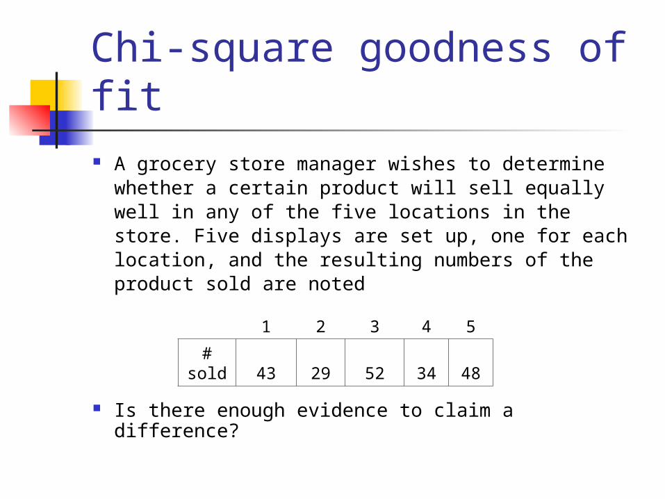
Chi-square goodness of fit A grocery store manager wishes to determine

whether a certain product will sell equally well in any of the five locations in the store. Five displays are set up, one for each location, and the resulting numbers of the product sold are noted

Is there enough evidence to claim a difference?

1 2 3 4 5

# sold 43 29 52 34 48

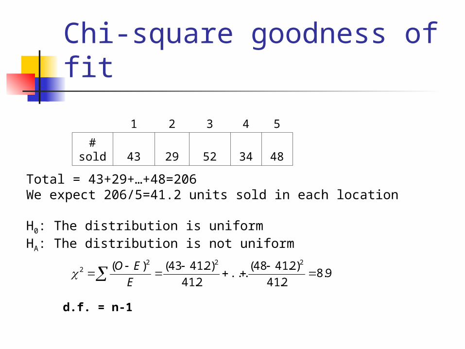
Chi-square goodness of fit

1 2 3 4 5

# sold 43 29 52 34 48

Total = 43+29+…+48=206We expect 206/5=41.2 units sold in each location

H0: The distribution is uniformHA: The distribution is not uniform

9.82.41

)2.4148(...

2.41

)2.4143()( 2222

E

EO

d.f. = n-1

Problem 35

A geneticist claims that four species of fruit flies should appear in the ratio of 1:3:3:9. Suppose that a sample of 4000 fruit flies contained 226, 764, 733, and 2277 flies of each species, respectively. At the 10% significance level, is there sufficient evidence to reject the geneticist’s hypothesis?

Chi-square test: warning Chi-square test is applicable only if the

expected value in each cell is greater than 5 (Compare to Binomial Distribution)

If this doesn’t hold, you might find Fisher exact test more useful

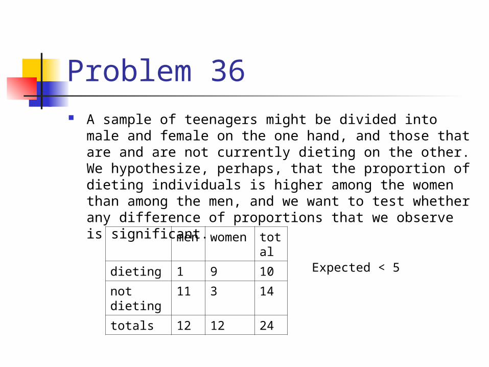
Problem 36 A sample of teenagers might be divided into male and

female on the one hand, and those that are and are not currently dieting on the other. We hypothesize, perhaps, that the proportion of dieting individuals is higher among the women than among the men, and we want to test whether any difference of proportions that we observe is significant.

men women total

dieting 1 9 10

not dieting 11 3 14

totals 12 12 24

Expected < 5

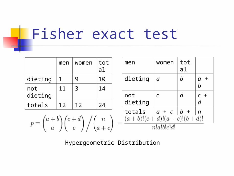
Fisher exact test

men women total

dieting 1 9 10

not dieting 11 3 14

totals 12 12 24

men women total

dieting a b a + b

not dieting c d c + d

totals a + c b + d n

Hypergeometric Distribution

Statistics

Part IV: Regression and ANOVA

The least squares line A simple data set consists of data pairs

(xi, yi), i = 1, ..., n, where xi is an independent variable and yi is a dependent variable

The model function has the formy = a + bx

We wish to find a and b for which the model "best" fits the data.

Residuals The least squares method defines "best"

as when S = Σ ri2 is at minimum.

A residual ri is defined as the difference between the values of the dependent variable and the predicted values from the estimated model

ri =yi - (a + b xi)

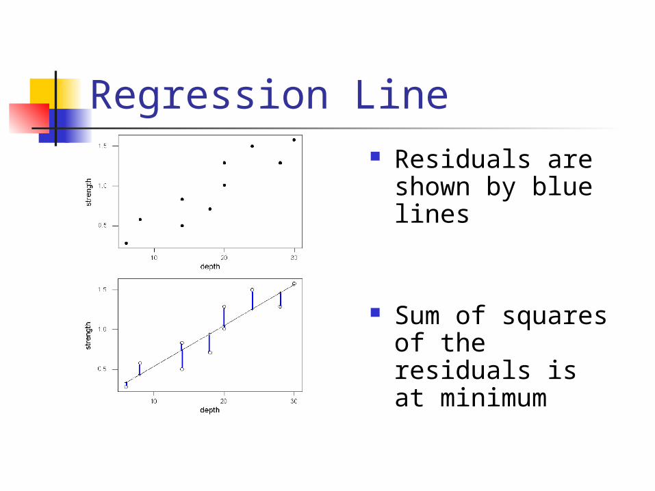
Regression Line Residuals are

shown by blue lines

Sum of squares of the residuals is at minimum

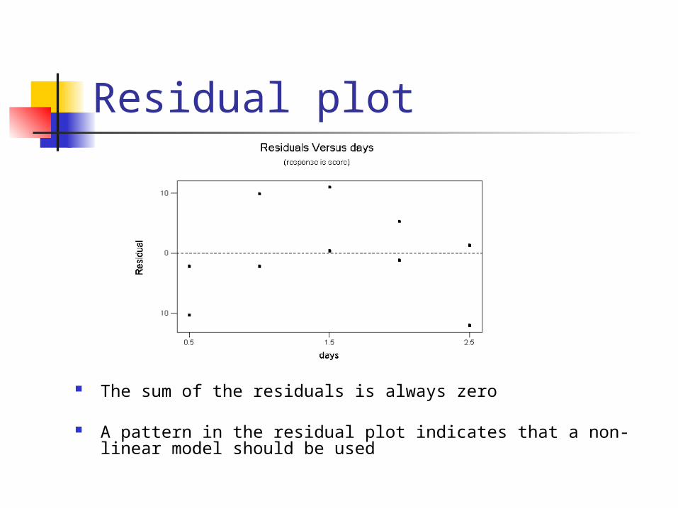
Residual plot

The sum of the residuals is always zero

A pattern in the residual plot indicates that a non-linear model should be used

Influential scores and outliers

In regression, an outlier is a data point with large residual

An influential score is the data point which significantly influences the regression line

If an influential score is removed from the sample, the regression line will change significantly

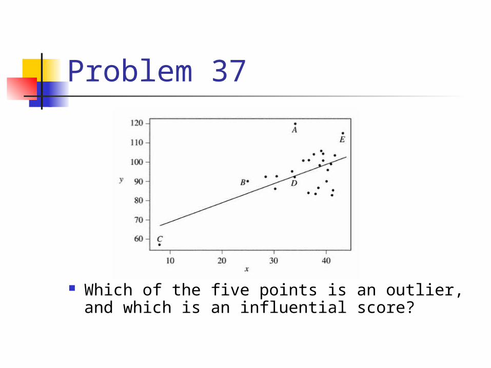
Problem 37

Which of the five points is an outlier, and which is an influential score?

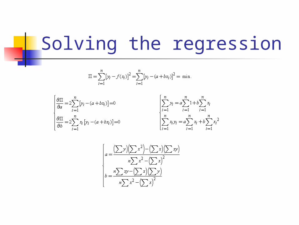
Solving the regression

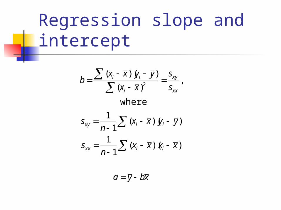
Regression slope and intercept

xbya

xxxxn

s

yyxxn

s

s

s

xx

yyxxb

iixx

iixy

xx

xy

i

ii

))((1

1

))((1

1

where

,)(

))((2

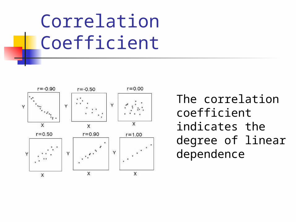
Correlation Coefficient

The correlation coefficient indicates the degree of linear dependence

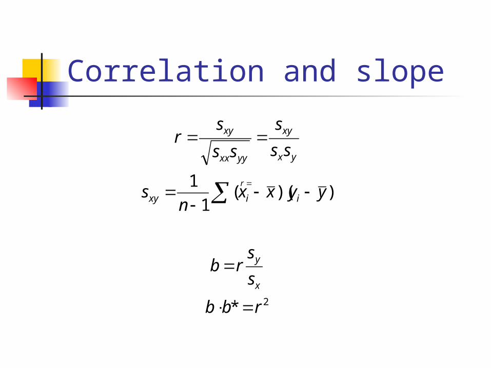
Correlation and slope

r

2*

))((1

1

rbb

s

srb

yyxxn

s

ss

s

ss

sr

x

y

iixy

yx

xy

yyxx

xy

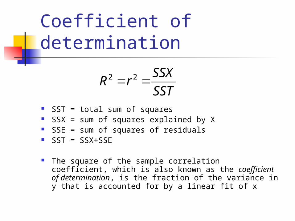
Coefficient of determination

SST = total sum of squares SSX = sum of squares explained by X SSE = sum of squares of residuals SST = SSX+SSE

The square of the sample correlation coefficient, which is also known as the coefficient of determination, is the fraction of the variance in y that is accounted for by a linear fit of x

SST

SSXrR 22

Sums of squares

SSESSX

termctcrossproduYYYY

YYYYYYsn

ii

iiiY

22

222

)ˆ()ˆ(

)ˆˆ()()1(

iY

iY red

blue

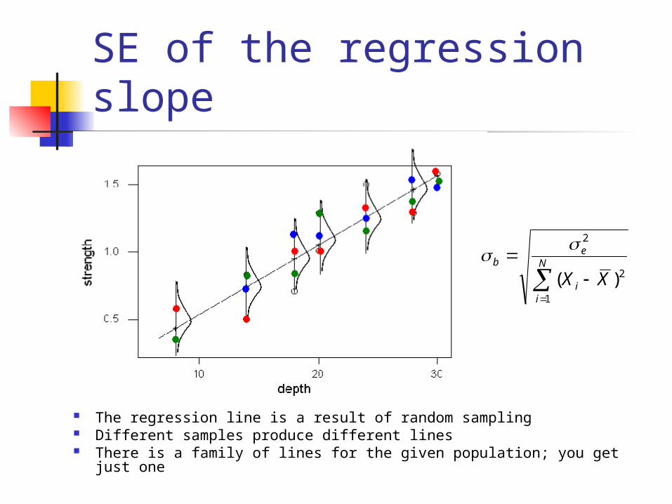
SE of the regression slope

The regression line is a result of random sampling Different samples produce different lines There is a family of lines for the given population; you get just one

N

ii

eb

XX1

2

2

)(

SE of the regression slope

N

ii

eb

XX1

2

2

)(

MSEn

SSEe

2

where σe is the standard deviation of the regression error

N

ii

b

XX

MSE

1

2)(

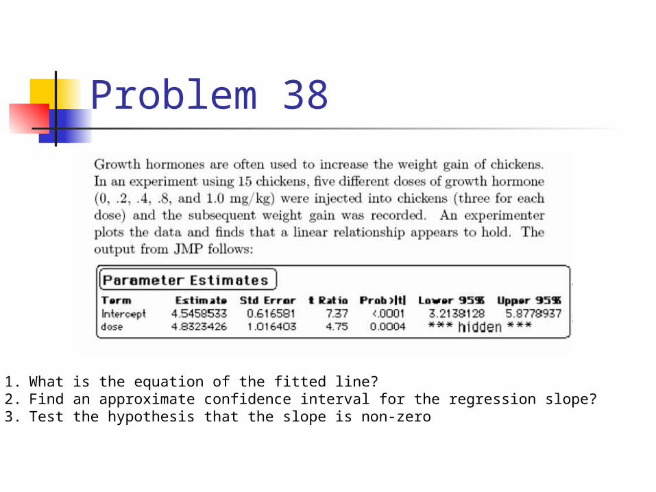
Problem 38

1. What is the equation of the fitted line?2. Find an approximate confidence interval for the regression slope?3. Test the hypothesis that the slope is non-zero

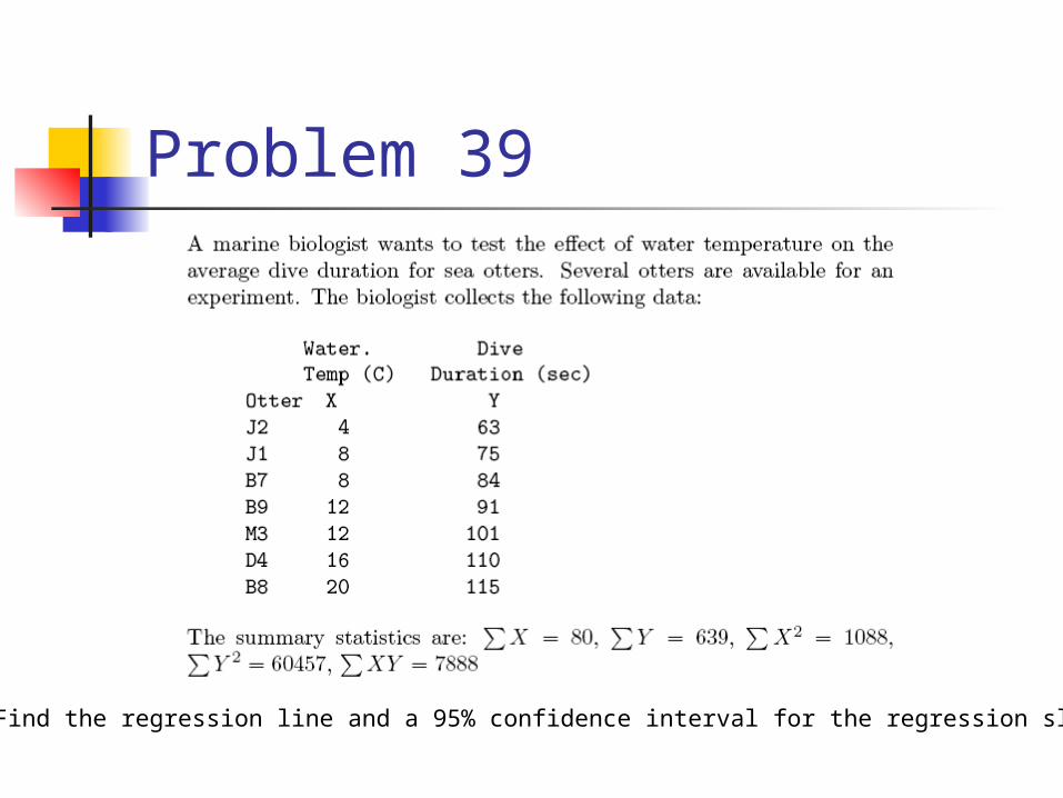
Problem 39

Find the regression line and a 95% confidence interval for the regression slope.

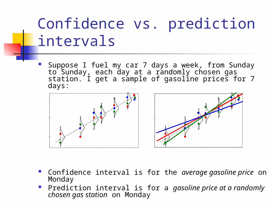
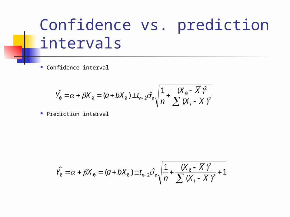
Confidence vs. prediction intervals Suppose I fuel my car 7 days a week, from Sunday to

Sunday, each day at a randomly chosen gas station. I get a sample of gasoline prices for 7 days:

Confidence interval is for the average gasoline price on Monday

Prediction interval is for a gasoline price at a randomly chosen gas station on Monday

Confidence interval

Prediction interval

Confidence vs. prediction intervals

2

20

2000 )(

)(1ˆ)(ˆ

XX

XX

ntbXaXY

ien

1)(

)(1ˆ)(ˆ

2

20

2000

XX

XX

ntbXaXY

ien

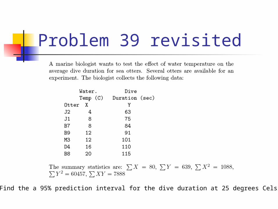
Problem 39 revisited

Find the a 95% prediction interval for the dive duration at 25 degrees Celsius

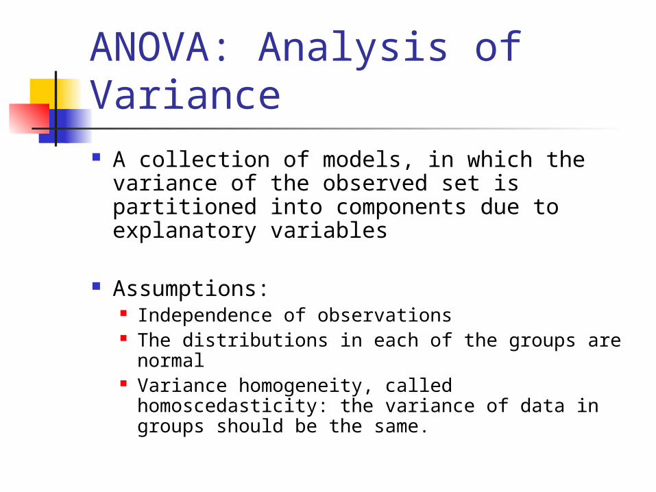
ANOVA: Analysis of Variance A collection of models, in which the variance

of the observed set is partitioned into components due to explanatory variables

Assumptions: Independence of observations The distributions in each of the groups are

normal Variance homogeneity, called homoscedasticity:

the variance of data in groups should be the same.

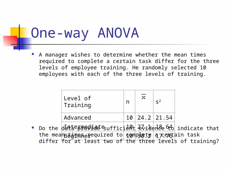
One-way ANOVA A manager wishes to determine whether the mean times

required to complete a certain task differ for the three levels of employee training. He randomly selected 10 employees with each of the three levels of training.

Do the data provide sufficient evidence to indicate that the mean times required to complete a certain task differ for at least two of the three levels of training?

Level of Training n       s2

Advanced 10

24.2 21.54

Intermediate 10

27.1 18.64

Beginner 10

30.2 17.76

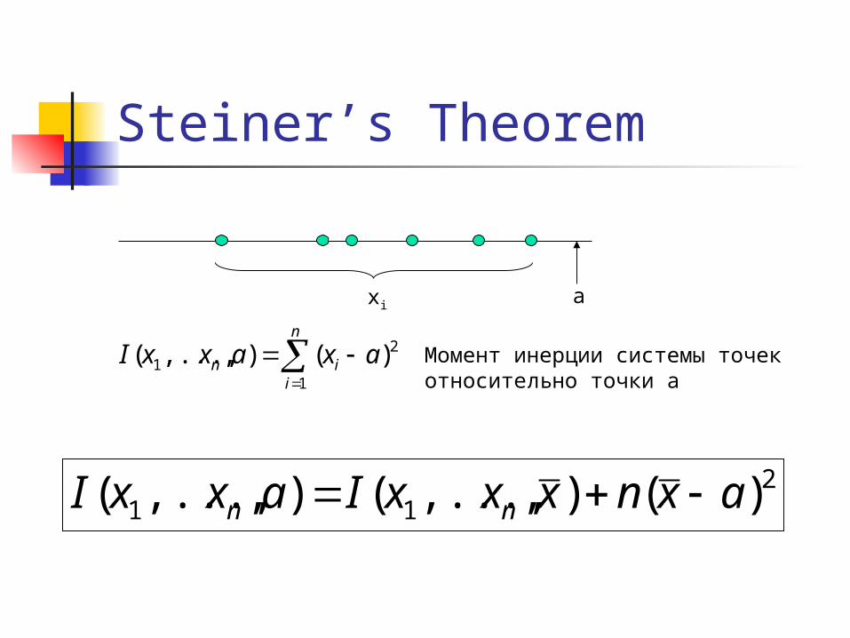
Steiner’s Theorem

n

iin axaxxI

1

21 )(),,...,(

axi

211 )(),,...,(),,...,( axnxxxIaxxI nn

Момент инерции системы точек относительно точки а

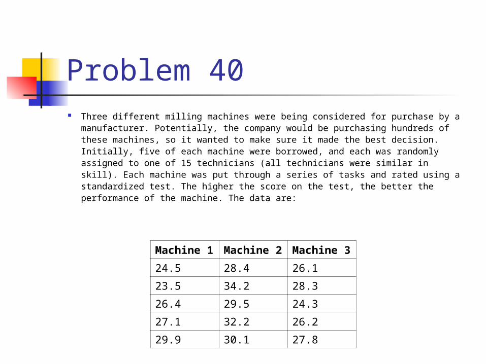
Problem 40 Three different milling machines were being considered for purchase by a

manufacturer. Potentially, the company would be purchasing hundreds of these machines, so it wanted to make sure it made the best decision. Initially, five of each machine were borrowed, and each was randomly assigned to one of 15 technicians (all technicians were similar in skill). Each machine was put through a series of tasks and rated using a standardized test. The higher the score on the test, the better the performance of the machine. The data are:

Machine 1 Machine 2 Machine 3

24.5 28.4 26.1

23.5 34.2 28.3

26.4 29.5 24.3

27.1 32.2 26.2

29.9 30.1 27.8

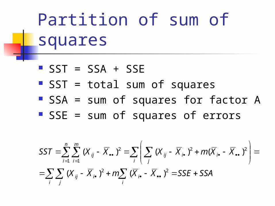
Partition of sum of squares SST = SSA + SSE SST = total sum of squares SSA = sum of squares for factor A SSE = sum of squares of errors

SSASSEXXmXX

XXmXXXXSST

ii

i jiij

i jiiij

n

i

m

iij

22

22

1 1

2

)()(

)()()(

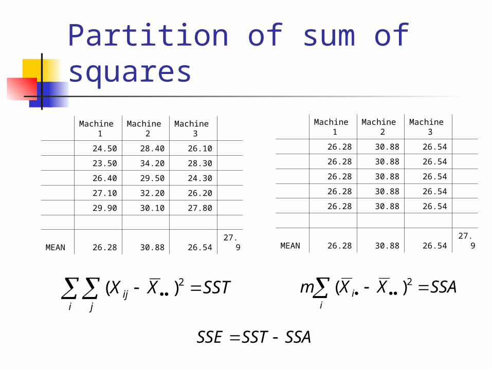
Partition of sum of squares

Machine 1

Machine 2

Machine 3

24.50 28.40 26.10

23.50 34.20 28.30

26.40 29.50 24.30

27.10 32.20 26.20

29.90 30.10 27.80

MEAN 26.28 30.88 26.54 27.9

Machine 1

Machine 2

Machine 3

26.28 30.88 26.54

26.28 30.88 26.54

26.28 30.88 26.54

26.28 30.88 26.54

26.28 30.88 26.54

MEAN 26.28 30.88 26.54 27.9

SSTXXi j

ij 2)(

ii SSAXXm 2)(

SSASSTSSE

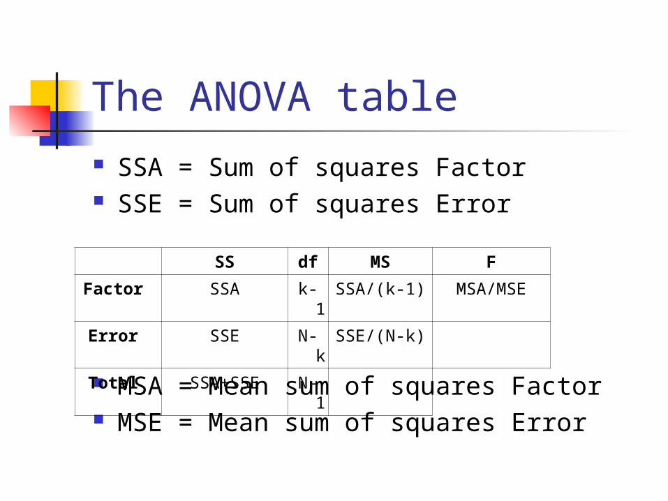
The ANOVA table SSA = Sum of squares Factor SSE = Sum of squares Error

MSA = Mean sum of squares Factor MSE = Mean sum of squares Error

SS df MS F

Factor SSA k-1 SSA/(k-1) MSA/MSE

Error SSE N-k SSE/(N-k) .

Total SSA+SSE N-1 .

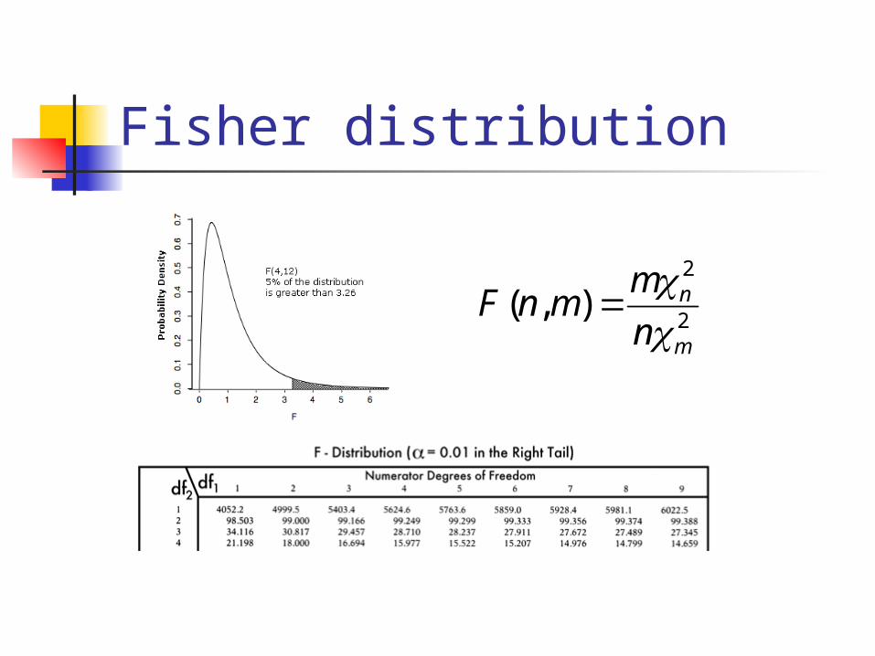
Fisher distribution

2

2

),(m

n

n

mmnF

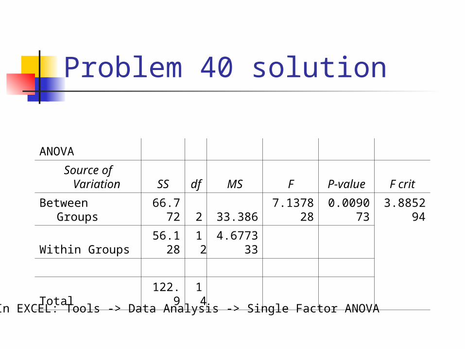
Problem 40 solution

ANOVA

Source of Variation SS df MS F P-value F crit

Between Groups 66.772 2 33.386 7.137828 0.009073 3.885294

Within Groups 56.128 12 4.677333

Total 122.9 14        

In EXCEL: Tools -> Data Analysis -> Single Factor ANOVA

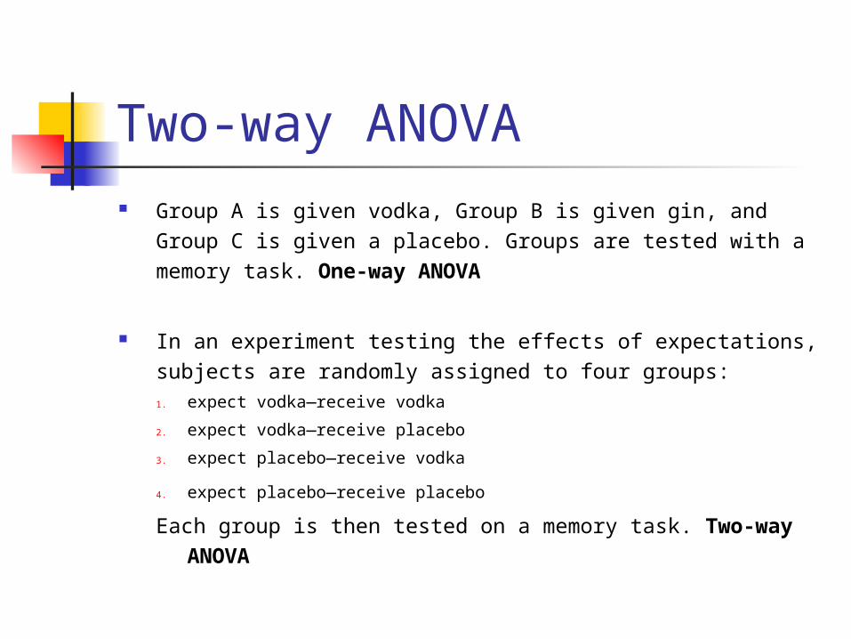
Two-way ANOVA Group A is given vodka, Group B is given gin, and Group

C is given a placebo. Groups are tested with a memory task. One-way ANOVA

In an experiment testing the effects of expectations, subjects are randomly assigned to four groups:1. expect vodka—receive vodka

2. expect vodka—receive placebo

3. expect placebo—receive vodka

4. expect placebo—receive placebo

Each group is then tested on a memory task. Two-way ANOVA

Partition of sum of squares

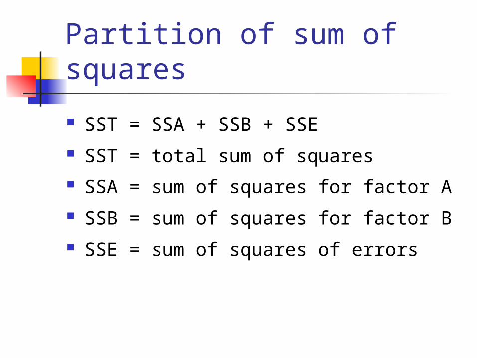
SST = SSA + SSB + SSE SST = total sum of squares SSA = sum of squares for factor A SSB = sum of squares for factor B SSE = sum of squares of errors

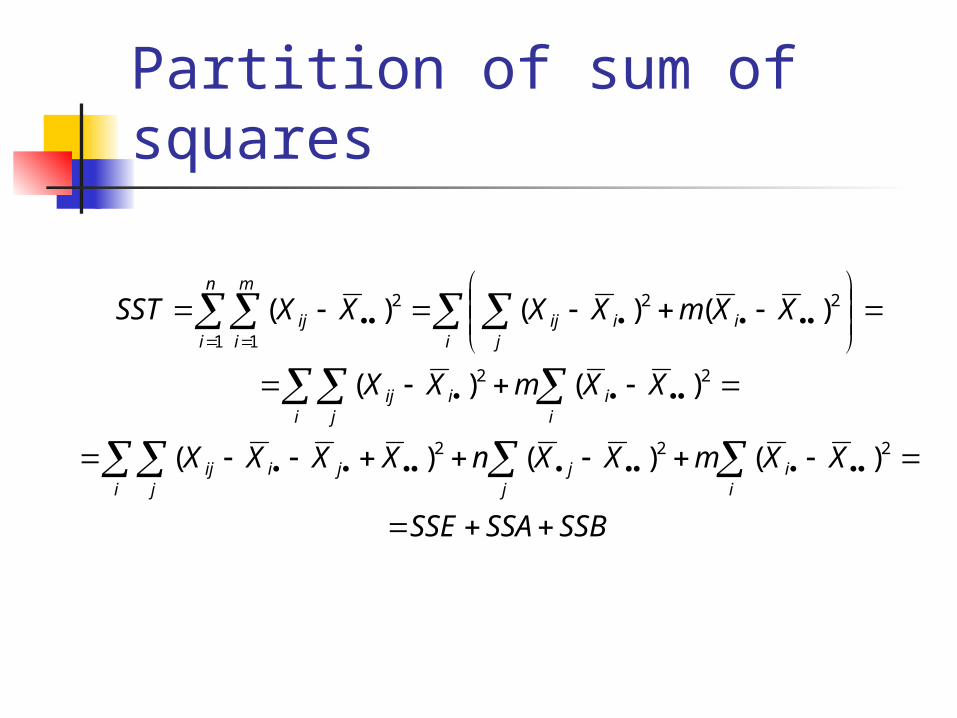
Partition of sum of squares

SSBSSASSE

XXmXXnXXXX

XXmXX

XXmXXXXSST

ii

jj

i jjiij

ii

i jiij

i jiiij

n

i

m

iij

222

22

22

1 1

2

)()()(

)()(

)()()(

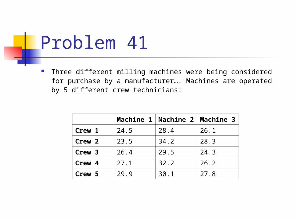
Problem 41 Three different milling machines were being considered for

purchase by a manufacturer…. Machines are operated by 5 different crew technicians:

Machine 1 Machine 2 Machine 3

Crew 1 24.5 28.4 26.1

Crew 2 23.5 34.2 28.3

Crew 3 26.4 29.5 24.3

Crew 4 27.1 32.2 26.2

Crew 5 29.9 30.1 27.8

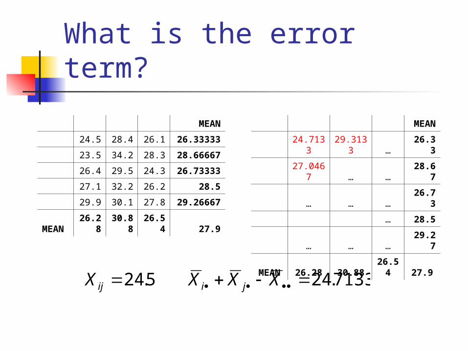
What is the error term?

MEAN

24.5 28.4 26.1 26.33333

23.5 34.2 28.3 28.66667

26.4 29.5 24.3 26.73333

27.1 32.2 26.2 28.5

29.9 30.1 27.8 29.26667

MEAN 26.28 30.88 26.54 27.9

        MEAN

 24.713

329.313

3 … 26.33

 27.046

7 … … 28.67

  … … … 26.73

      … 28.5

  … … … 29.27

MEAN 26.28 30.88 26.54 27.9

7133.245.24 XXXX jiij

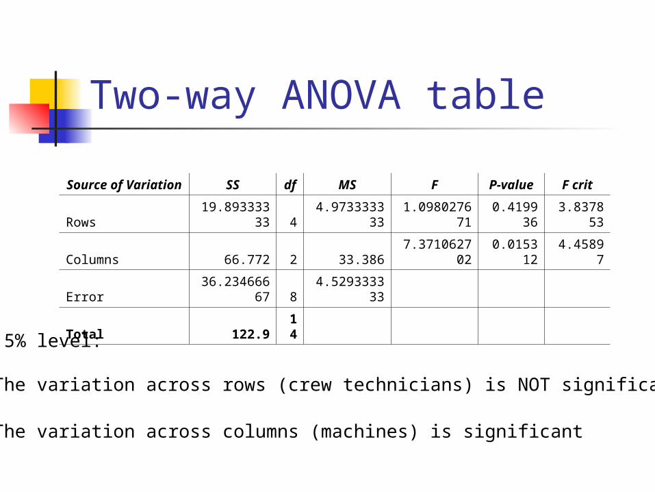
Two-way ANOVA table

Source of Variation SS df MS F P-value F crit

Rows19.8933333

3 44.97333333

31.09802767

10.41993

63.83785

3

Columns 66.772 2 33.3867.37106270

20.01531

2 4.45897

Error36.2346666

7 84.52933333

3

Total 122.9 14At 5% level:

• The variation across rows (crew technicians) is NOT significant

• The variation across columns (machines) is significant

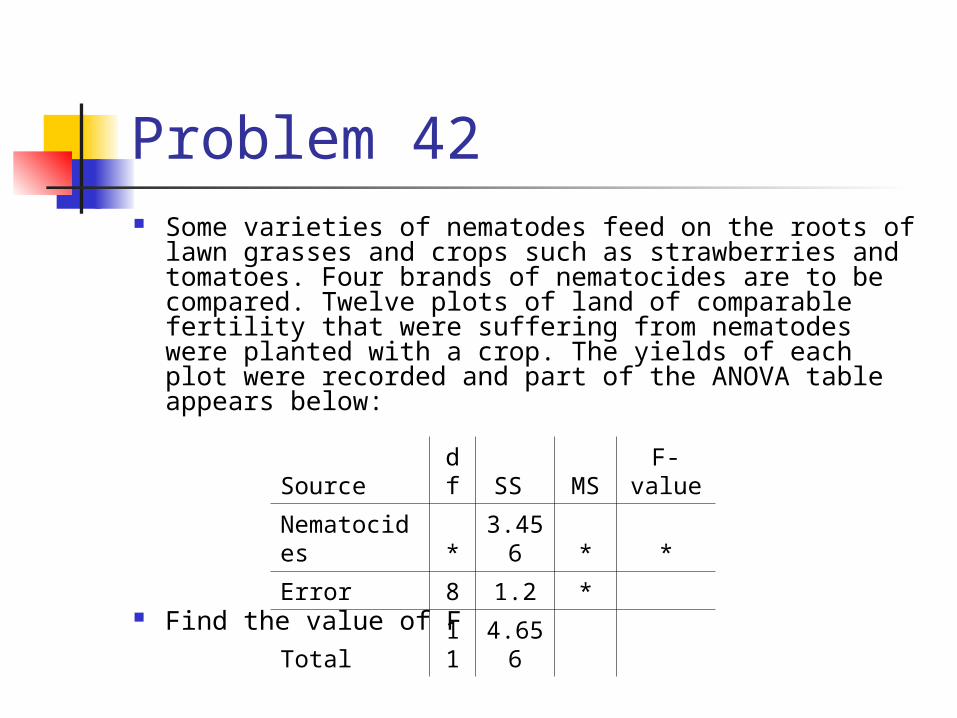
Problem 42 Some varieties of nematodes feed on the roots of

lawn grasses and crops such as strawberries and tomatoes. Four brands of nematocides are to be compared. Twelve plots of land of comparable fertility that were suffering from nematodes were planted with a crop. The yields of each plot were recorded and part of the ANOVA table appears below:

Find the value of F

Source df SS MS F-value

Nematocides * 3.456 * *

Error 8 1.2 *

Total 11 4.656

THE END

Extra Problems

All bags entering a research facility are screened. Ninety-seven percent of the bags that contain forbidden material trigger an alarm. Fifteen percent of the bags that do not contain forbidden material also trigger the alarm. If 1 out of every 1,000 bags entering the building contains forbidden material, what is the probability that a bag that triggers the alarm will actually contain forbidden material?

Extra problems

Pepper plants watered lightly every day for a month show an average growth of 27 cm with the standard deviation of 8.3 cm, while pepper plants watered heavily once a week for a month show an average growth of 29 cm with the standard deviation of 7.9 cm. In a sample of 60 plants, half of which were given each of the water treatments, what is the probability that the difference in average growth between the two halves is between -3 and + 3 cm?