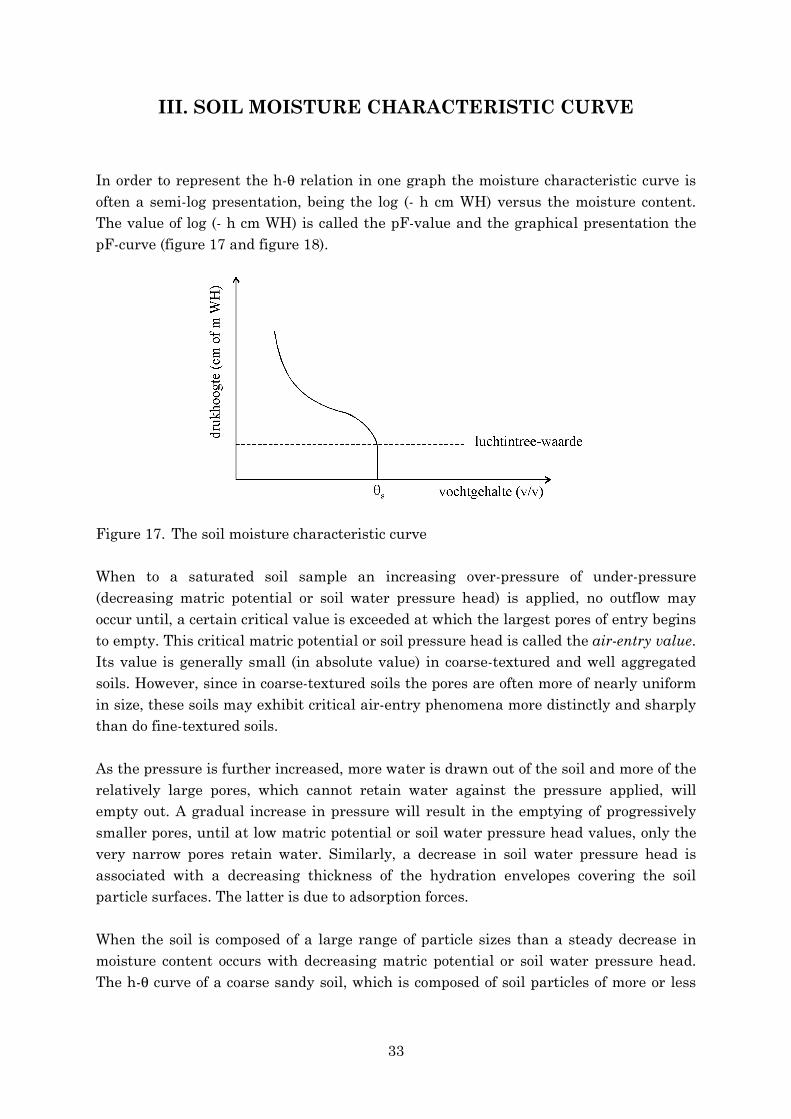
33

III. SOIL MOISTURE CHARACTERISTIC CURVE

In order to represent the h-θ relation in one graph the moisture characteristic curve isoften a semi-log presentation, being the log (- h cm WH) versus the moisture content.The value of log (- h cm WH) is called the pF-value and the graphical presentation thepF-curve (figure 17 and figure 18).

Figure 17. The soil moisture characteristic curve

When to a saturated soil sample an increasing over-pressure of under-pressure(decreasing matric potential or soil water pressure head) is applied, no outflow mayoccur until, a certain critical value is exceeded at which the largest pores of entry beginsto empty. This critical matric potential or soil pressure head is called the air-entry value.Its value is generally small (in absolute value) in coarse-textured and well aggregatedsoils. However, since in coarse-textured soils the pores are often more of nearly uniformin size, these soils may exhibit critical air-entry phenomena more distinctly and sharplythan do fine-textured soils.

As the pressure is further increased, more water is drawn out of the soil and more of therelatively large pores, which cannot retain water against the pressure applied, willempty out. A gradual increase in pressure will result in the emptying of progressivelysmaller pores, until at low matric potential or soil water pressure head values, only thevery narrow pores retain water. Similarly, a decrease in soil water pressure head isassociated with a decreasing thickness of the hydration envelopes covering the soilparticle surfaces. The latter is due to adsorption forces.

When the soil is composed of a large range of particle sizes than a steady decrease inmoisture content occurs with decreasing matric potential or soil water pressure head.The h-θ curve of a coarse sandy soil, which is composed of soil particles of more or less

34

equal size, however shows a plateau because it consists of a large amount of large poresof equivalent diameter which are emptied at a specific soil water pressure head.

Increasing the applied pressure is thus associated with decreasing soil wetness. Theamount of water remaining in the soil at equilibrium is a function of the sizes andvolumes of the water-filled pores and hence it is function of the soil water pressure head.This function is usually measured experimentally and it is represented graphically by acurve known as the soil-moisture retention curve, or the soil moisture characteristic.

Recalling the capillary equation the equivalent diameter (d) of the pores which areemptied at a specific soil water pressure head e.g. - 0,3 m equals:

µm100m10.110.3,0.10

075,0.4gh.2.2r2d 4

3w

=≈=ρ

γ== −

This relation is valid for non-swelling soils and moreover gives only a rough idea sincethe pores are in reality not always spherical cavities interconnected by straightcapillaries.

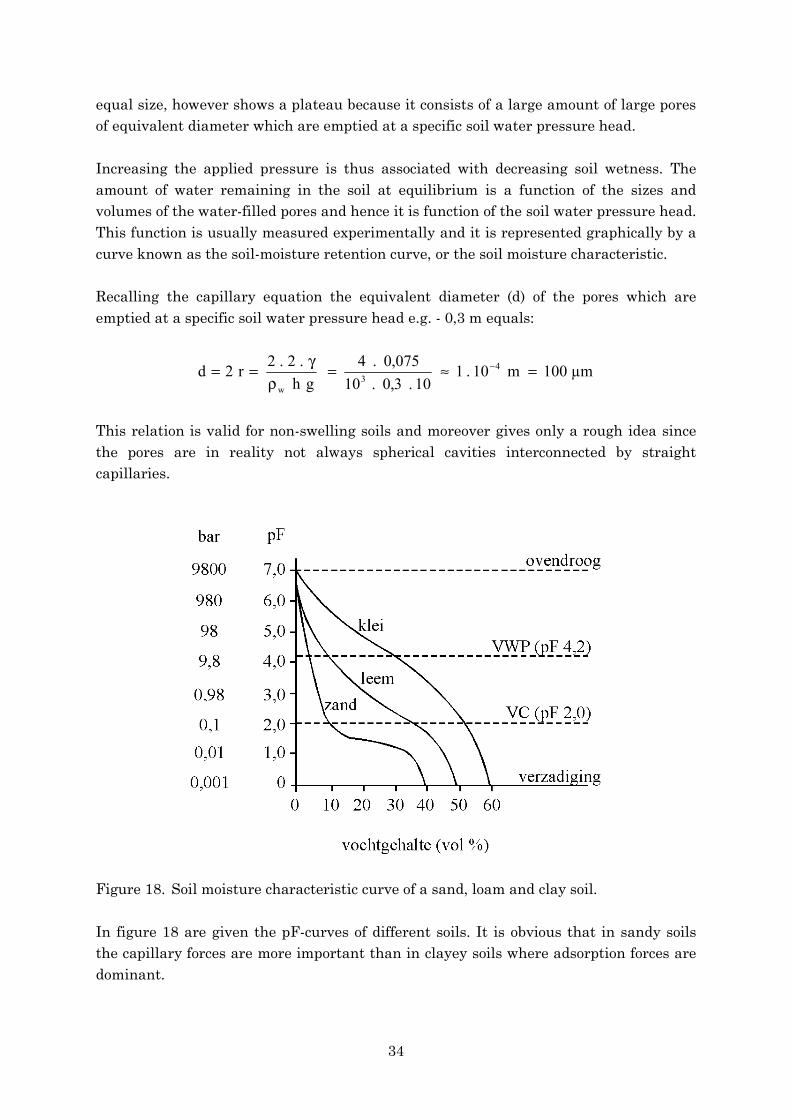
Figure 18. Soil moisture characteristic curve of a sand, loam and clay soil.

In figure 18 are given the pF-curves of different soils. It is obvious that in sandy soilsthe capillary forces are more important than in clayey soils where adsorption forces aredominant.

35

Apart from the particle size distribution (texture), also the soil structure (pore geometry)affects the shape of the soil moisture characteristic curve, particularly in the wet range(high soil water pressure head range). The amount of water retained at relatively highmatric potential (say between 0 and – 1 bar) depends primarily upon the capillary effectand the pore size distribution, and hence is strongly affected by the structure of the soil.On the other hand, water retention in the low matric potential range is due increasinglyto adsorption and is thus influenced less by the structure and more by the texture andspecific surface of the soil material. The water content at a matric potential of – 15 bar(often taken to be the lower limit of soil moisture availability to plants) is fairly wellcorrelated with the surface area of a soil and would represent, roughly about 10molecular layers of water if it ware distributed uniformly over the particle surfaces.

It should be obvious from the foregoing that the soil moisture characteristic curve isstrongly affected by soil texture. The greater the clay content, in general, the greater thewater retention at any particular matric potential, and the more gradual the slope of thecurve. In a sandy soil, moist of the pores are relatively large, and once the large poresare emptied at a given matric potential, only a small amount of water remains. In aclayey soil, the pore size distribution is more uniform, and more of the water isadsorbed, so that decreasing the matric potential causes a more gradual decrease inwater content (Figure 18).

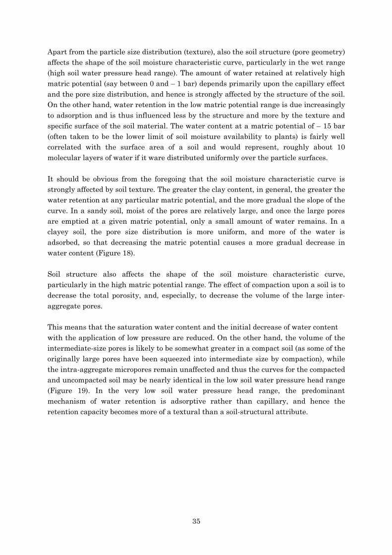
Soil structure also affects the shape of the soil moisture characteristic curve,particularly in the high matric potential range. The effect of compaction upon a soil is todecrease the total porosity, and, especially, to decrease the volume of the large inter-aggregate pores.

This means that the saturation water content and the initial decrease of water contentwith the application of low pressure are reduced. On the other hand, the volume of theintermediate-size pores is likely to be somewhat greater in a compact soil (as some of theoriginally large pores have been squeezed into intermediate size by compaction), whilethe intra-aggregate micropores remain unaffected and thus the curves for the compactedand uncompacted soil may be nearly identical in the low soil water pressure head range(Figure 19). In the very low soil water pressure head range, the predominantmechanism of water retention is adsorptive rather than capillary, and hence theretention capacity becomes more of a textural than a soil-structural attribute.

36

Figure 19. The effect of soil structure on soil water retention.

Therefore it is important to determine the soil moisture characteristic curve onundisturbed samples. The inverse of the slope of the curve, which is the change of watercontent per unit change of matric potential, is generally termed the differential (orspecific) water capacity "C (θ)":

dhd)(C θ=θ

This is an important property in relation to soil moisture storage and availability toplants as water transport in general. The actual value of C (θ) depends upon the wetnessrange, the texture and the hysteresis effect.

The estimation of the relation between the matric potential versus the moisture contentbased on soil properties is not always successful (see chapter IV). The adsorption andpore geometry effects are often too complex to be described by a simple model.

3.1. Determination of the soil moisture characteristic curve.

The determination of the soil moisture characteristic curves as presented in Figure 18,is carried out in the laboratory through a systematic desorption of water starting from asaturated soil sample. As mentioned earlier the determination should be carried out onundisturbed soil samples, certainly at high soil water pressure heads (0 till -1/3 atm.).At lower soil water pressure heads the influence of soil structure on the further shape ofthe curve (ψm(h) - θ relation) is negligible.

37

The methods consists in the determination of the water content of the soil sample at themoment that hydraulic equilibrium is reached for a certain applied matric potential. Ittakes mostly some days before equilibrium is reached depending on the particle sizedistribution, size of the sample and the applied pressure.

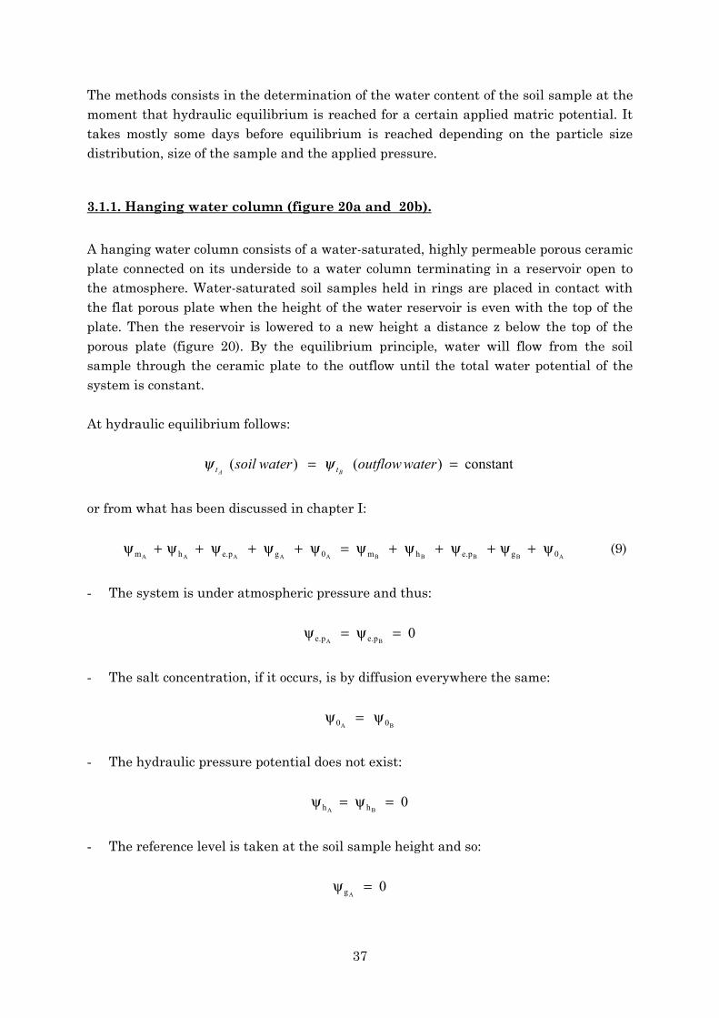
3.1.1. Hanging water column (figure 20a and 20b).

A hanging water column consists of a water-saturated, highly permeable porous ceramicplate connected on its underside to a water column terminating in a reservoir open tothe atmosphere. Water-saturated soil samples held in rings are placed in contact withthe flat porous plate when the height of the water reservoir is even with the top of theplate. Then the reservoir is lowered to a new height a distance z below the top of theporous plate (figure 20). By the equilibrium principle, water will flow from the soilsample through the ceramic plate to the outflow until the total water potential of thesystem is constant.

At hydraulic equilibrium follows:

constant)()( == wateroutflowwatersoilBA tt ψψ

or from what has been discussed in chapter I:

ABBBBAAAAA 0gp.ehm0gp.ehm ψ+ψ+ψ+ψ+ψ=ψ+ψ+ψ+ψ+ψ (9)

- The system is under atmospheric pressure and thus:

0BA p.ep.e =ψ=ψ

- The salt concentration, if it occurs, is by diffusion everywhere the same:

BA 00 ψ=ψ

- The hydraulic pressure potential does not exist:

0BA hh =ψ=ψ

- The reference level is taken at the soil sample height and so:

0Ag

=ψ

38

- At the outflow : 0Bm

=ψ , so that eq. (9) becomes:

hg1

g1of

BABA gmgm −=ψ=ψψ=ψ

At equilibrium the moisture content (θ) is determined and one obtains consequently onepoint of the soil moisture characteristic curve (h1 - θ1).

As the tube is adjustable, different under-pressures or matric potentials can be applied,whereby the air entry value of the porous ceramic plate may not be exceeded. The lowestmatric potential that can be applied by this method is similar to that for a tensiometerbeing ≈ - 8 m WH.

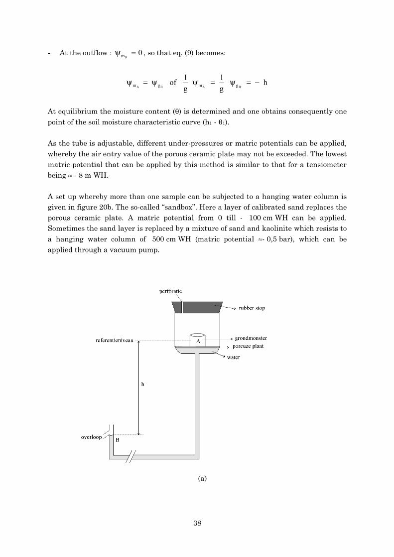
A set up whereby more than one sample can be subjected to a hanging water column isgiven in figure 20b. The so-called “sandbox”. Here a layer of calibrated sand replaces theporous ceramic plate. A matric potential from 0 till - 100 cm WH can be applied.Sometimes the sand layer is replaced by a mixture of sand and kaolinite which resists toa hanging water column of 500 cm WH (matric potential ≈- 0,5 bar), which can beapplied through a vacuum pump.

(a)

39

(b)

Figure 20. Desaturation of saturated soil samples to a desired energy state with ahanging water column.

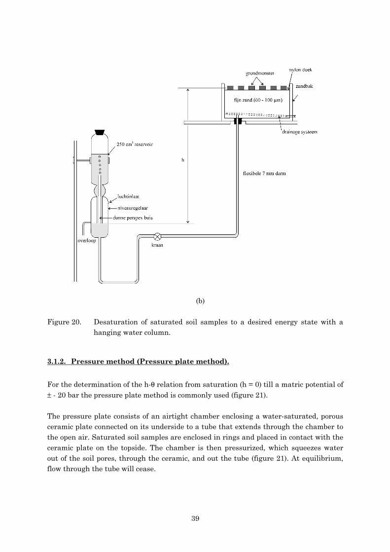
3.1.2. Pressure method (Pressure plate method).

For the determination of the h-θ relation from saturation (h = 0) till a matric potential of± - 20 bar the pressure plate method is commonly used (figure 21).

The pressure plate consists of an airtight chamber enclosing a water-saturated, porousceramic plate connected on its underside to a tube that extends through the chamber tothe open air. Saturated soil samples are enclosed in rings and placed in contact with theceramic plate on the topside. The chamber is then pressurized, which squeezes waterout of the soil pores, through the ceramic, and out the tube (figure 21). At equilibrium,flow through the tube will cease.

40

Figure 21. Desaturation of saturated soil samples to a desired energy state with apressure plate.

At hydraulic equilibrium:

constant==BA tt ψψ

- Salt, if present, diffusion occurs through the porous plate and:

BA 00 ψ=ψ

- No hydrostatic pressure is present or: 0BA hh =ψ=ψ

- In B we have free water ( 0Bm

=ψ ) under atmospheric pressure ( 0Bp.e

=ψ ).

- The differences in gravitational potential between A en B may be neglected so that:

BA gg ψ=ψ

(eventually = 0 if the reference level is taken at the level of the sample).

So the equation (9) becomes:

AAAA pempem or .... 0 ψψψψ −==+

41

When equilibrium is reached, the chamber may be depressurized and the water contentof the samples measured and one point of the h-θ relation is obtained. An assumption ismade in this method whereby the matric potential of the sample does not change as theair pressure is lowered to atmospheric.

This method may be used up to air gauge pressures of about 15 bars (pF = 4,2, beingpermanent wilting point, see 3.4) if special fine-pore ceramic plates are used. Since thesedevices have a very high flow resistance, it may require a substantial amount of time toremove the last small amount of water from the soil. Thus, the time of equilibrium isdifficult to estimate.

3.1.3. Vapor pressure equilibrium.

For matric potentials lower than – 15-bar vapor pressure equilibration of salt solutionsare used. By adding pre-calibrated amounts of certain salts, the energy level of areservoir of pure water may be lowered to any specified level. If this reservoir is broughtinto contact with a moist soil sample, water will flow through the vapor phase from thesample to the reservoir. If the sample and the reservoir are placed adjacent to eachother in a closed chamber at constant temperature, water will be exchanged through thevapor phase by evaporation from the soil sample and condensation in the reservoir untilequilibrium is reached. Since the reservoir is a pool of salt solution, at equilibrium thetotal potential will be ψt = ψso of the solution. In the soil ψt = ψm + ψo since the air-waterinterface acts as a solute membrane. Thus ψm = ψso - ψo, the difference between thesolute potentials of the reservoir and the soil. In practice, the soil will usually not besaline enough for its solute potential to be significant compared to ψo in the range wherethese measurements are made. Knowing that the relative humidity is related to the poolof salt solution one obtains that:

)(ln0

0 potentialwaterPP

MTR

wm ψψψ ==+ (10)

at t = 20°C, and with:R = 8,3 J mol-1 K-1

T = 273 + 20 = 293 K;M = 18 10-3 kg mol-1

P = vapor pressure of soil waterPo = saturated vapor pressure (vapor pressure of pure free water)

Equation 10 becomes:

0

5

030 log303,2.10.3,1ln

10.18293.3,8

PP

PP

m ≈≈+ −ψψ

42

)kgJ(PPlog10.3 1

0

50m

−≈ψ+ψ

)Pa(PPlog10.3)(0

80mw ≈ψ+ψρ

)m(PPlog10.3)(

g1

0

40m ≈ψ+ψ

or

hcmHRcmPP == )(

100log10.3)(log10.3 6

0

6

RH, being the relative humidity and equals 100 (P/P0). The relative vapor pressure P/P0

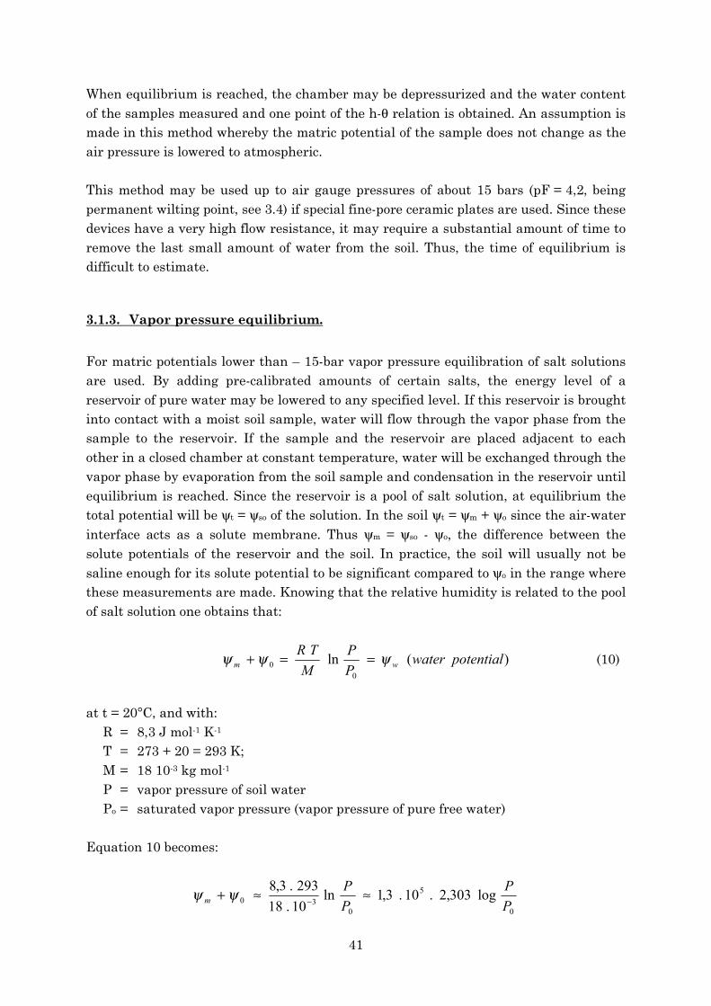
seems to be a measure of the sum of the matric and osmotic potential of the soil water. Itis now possible to describe the shape of the relation between the relative vapor pressureor relative humidity in function of pF-values (figure 22). From the equation

oom P

PMRT ln=+ ψψ

follows for a non-saline soil (ψo = 0)

om P

PMRT ln=ψ

or

)(log10.31 6 cmPPh

g om ==ψ

So finally one obtains:

)log10.3(log)(log 6

oPPhpF =−=

)100(loglog5,6HR

pF +=

)log2(log5,6 HRpF −+= (11)

43

Figure 22. Relation between relative humidity and pF-values.

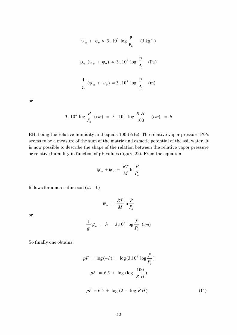
Using this relation, part of the moisture characteristic can be established. The methodconsists of putting in a closed environment, containing a salt saturated solution, a soilsample (figure 23). Water transport will take place through the vapor phase untilequilibrium will be reached between the ψt of the soil water and the ψt of the water inthe vapor phase. Equilibrium is reached when a constant weight of the soil sample isreached. At that moment the moisture content is determined.

From figure 22 it is clear that within the range of 10% to 75% R.H. the relation is almostlinear and very steep which shows that a change in R.H. has only a relative small effecton the pF-value (range of pF = 5,5 till pF = 6,5). On the other hand in the low pF-range(important for plant growth), a small change in R.H. results in a relative large change inpF-values. Since changes in temperature strongly influence the shape of the curve inthat range this technique is only applicable to establish the h-θ relation in the range >pF ± 5. To obtain a certain vapor pressure a specific salt saturated solution is used.

Figure 23. Set up to obtain a certain pF-value by means of vapour pressureequilibrium.

44

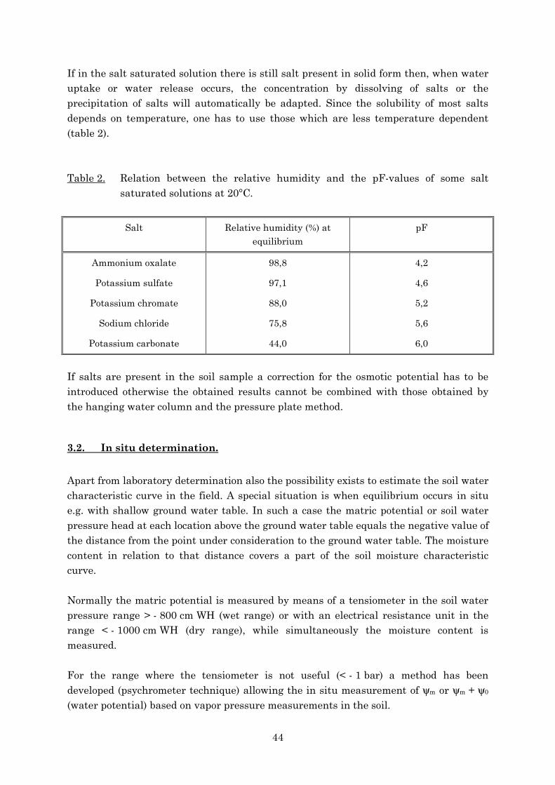
If in the salt saturated solution there is still salt present in solid form then, when wateruptake or water release occurs, the concentration by dissolving of salts or theprecipitation of salts will automatically be adapted. Since the solubility of most saltsdepends on temperature, one has to use those which are less temperature dependent(table 2).

Table 2. Relation between the relative humidity and the pF-values of some saltsaturated solutions at 20°C.

Salt Relative humidity (%) atequilibrium

pF

Ammonium oxalate

Potassium sulfate

Potassium chromate

Sodium chloride

Potassium carbonate

98,8

97,1

88,0

75,8

44,0

4,2

4,6

5,2

5,6

6,0

If salts are present in the soil sample a correction for the osmotic potential has to beintroduced otherwise the obtained results cannot be combined with those obtained bythe hanging water column and the pressure plate method.

3.2. In situ determination.

Apart from laboratory determination also the possibility exists to estimate the soil watercharacteristic curve in the field. A special situation is when equilibrium occurs in situe.g. with shallow ground water table. In such a case the matric potential or soil waterpressure head at each location above the ground water table equals the negative value ofthe distance from the point under consideration to the ground water table. The moisturecontent in relation to that distance covers a part of the soil moisture characteristiccurve.

Normally the matric potential is measured by means of a tensiometer in the soil waterpressure range > - 800 cm WH (wet range) or with an electrical resistance unit in therange < - 1000 cm WH (dry range), while simultaneously the moisture content ismeasured.

For the range where the tensiometer is not useful (< - 1 bar) a method has beendeveloped (psychrometer technique) allowing the in situ measurement of ψm or ψm + ψ0

(water potential) based on vapor pressure measurements in the soil.

45

At equilibrium, the potential of soil moisture is equal to the potential of the water vaporin the ambient air. If thermal equilibrium is assured and the gravitational effect isneglected, the vapor potential can be taken to be equal to the sum of the matric andosmotic potentials, since air acts as an ideal semi-permeable membrane in allowing onlywater molecules to pass.

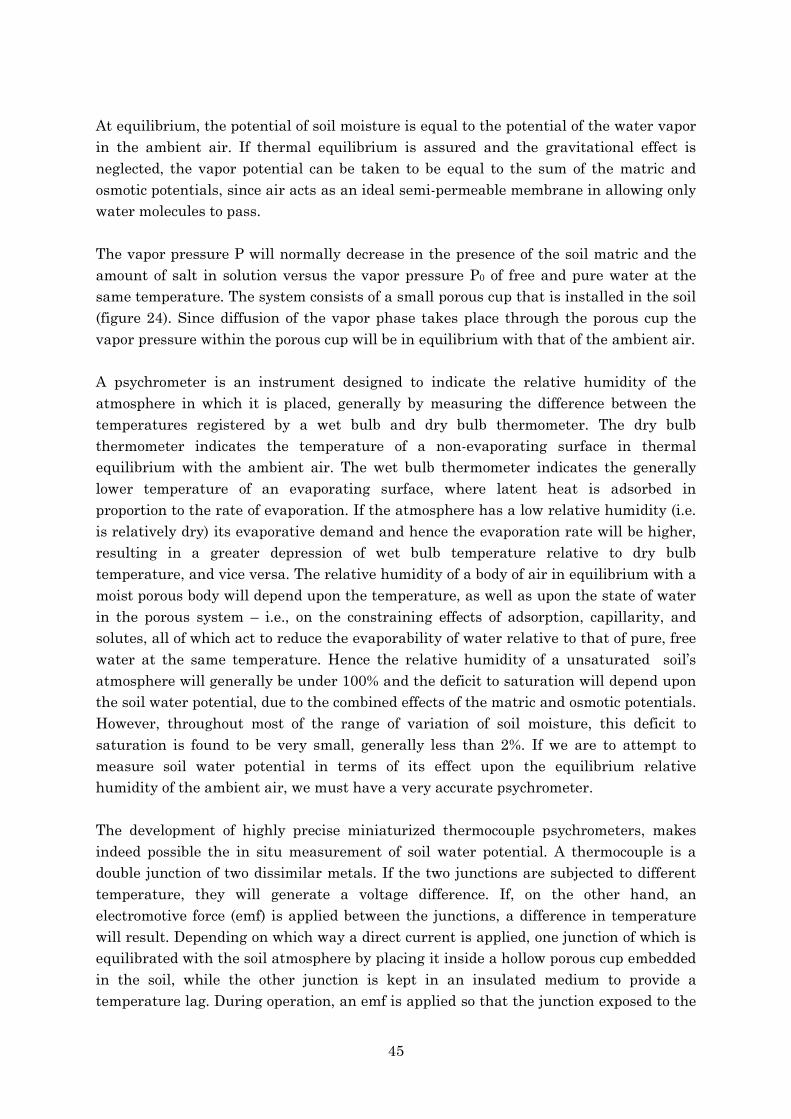
The vapor pressure P will normally decrease in the presence of the soil matric and theamount of salt in solution versus the vapor pressure P0 of free and pure water at thesame temperature. The system consists of a small porous cup that is installed in the soil(figure 24). Since diffusion of the vapor phase takes place through the porous cup thevapor pressure within the porous cup will be in equilibrium with that of the ambient air.

A psychrometer is an instrument designed to indicate the relative humidity of theatmosphere in which it is placed, generally by measuring the difference between thetemperatures registered by a wet bulb and dry bulb thermometer. The dry bulbthermometer indicates the temperature of a non-evaporating surface in thermalequilibrium with the ambient air. The wet bulb thermometer indicates the generallylower temperature of an evaporating surface, where latent heat is adsorbed inproportion to the rate of evaporation. If the atmosphere has a low relative humidity (i.e.is relatively dry) its evaporative demand and hence the evaporation rate will be higher,resulting in a greater depression of wet bulb temperature relative to dry bulbtemperature, and vice versa. The relative humidity of a body of air in equilibrium with amoist porous body will depend upon the temperature, as well as upon the state of waterin the porous system – i.e., on the constraining effects of adsorption, capillarity, andsolutes, all of which act to reduce the evaporability of water relative to that of pure, freewater at the same temperature. Hence the relative humidity of a unsaturated soil’satmosphere will generally be under 100% and the deficit to saturation will depend uponthe soil water potential, due to the combined effects of the matric and osmotic potentials.However, throughout most of the range of variation of soil moisture, this deficit tosaturation is found to be very small, generally less than 2%. If we are to attempt tomeasure soil water potential in terms of its effect upon the equilibrium relativehumidity of the ambient air, we must have a very accurate psychrometer.

The development of highly precise miniaturized thermocouple psychrometers, makesindeed possible the in situ measurement of soil water potential. A thermocouple is adouble junction of two dissimilar metals. If the two junctions are subjected to differenttemperature, they will generate a voltage difference. If, on the other hand, anelectromotive force (emf) is applied between the junctions, a difference in temperaturewill result. Depending on which way a direct current is applied, one junction of which isequilibrated with the soil atmosphere by placing it inside a hollow porous cup embeddedin the soil, while the other junction is kept in an insulated medium to provide atemperature lag. During operation, an emf is applied so that the junction exposed to the

46

soil atmosphere is cooled to a temperature below the dew point of that atmosphere, atwhich point a droplet of water condenses on the junction, allowing it to become, in effect,a wet bulb thermometer. This is a consequence of the so-called Peltier effect. The coolingis the stopped, and as the water from the droplet reevaporates the junction attains a wetbulb temperature which remains nearly constant until the junction dries out, afterwhich it returns to the ambient soil temperature. While evaporation takes place, thedifference in temperature between the wet bulb and the insulated junction serving asdry bulb generates an emf, which is indicative of the soil water potential.

The relative humidity (i.e. the vapor pressure depression relative to that of pure, freewater) is related to the soil water potential according to

)potentiaalwater(PPln

MTR

w0

0m ψ==ψ+ψ (12)

where P is the vapor pressure of soil water, Po the vapor pressure of pure free water atthe same temperature and air pressure, and R the gas constant for water vapor.

The measurement of vapor pressure or relative humidity is obviously highly sensitive totemperature changes. Hence the need for very accurate temperature control andmonitoring. Under field conditions, the accuracy claimed is of the order of about 0.5 barof soil water potential. The instrument is thus not practical at high soil water potential,but can be quite useful considerably beyond the suction range of the tensiometer. It isused mostly in research and manufactured commercially.

To measure the relative humidity a thermocouple of chromel/constantan is usedwhereby the cold junction is suspended in the porous cup while the other one is fixed inteflon to be used as reference and kept at constant temperature.

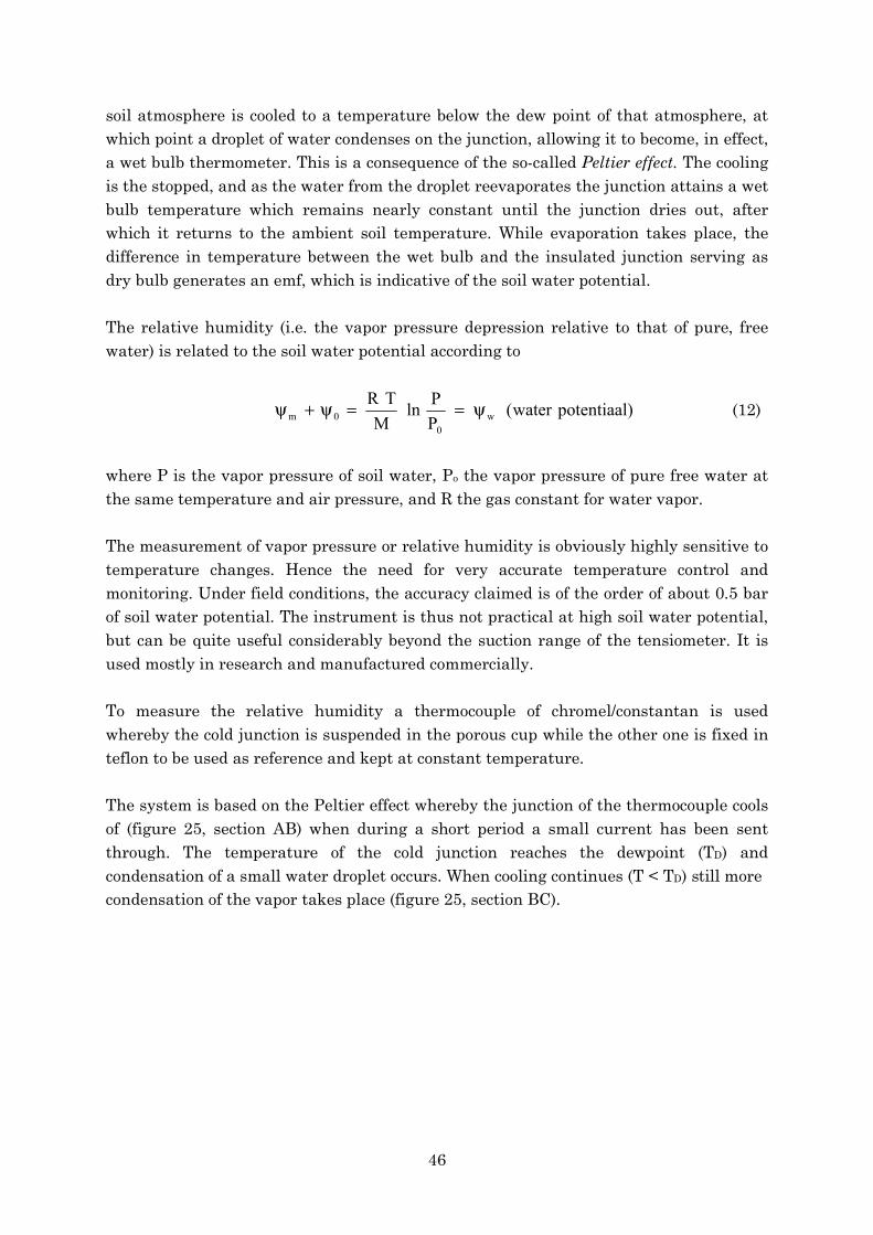
The system is based on the Peltier effect whereby the junction of the thermocouple coolsof (figure 25, section AB) when during a short period a small current has been sentthrough. The temperature of the cold junction reaches the dewpoint (TD) andcondensation of a small water droplet occurs. When cooling continues (T < TD) still morecondensation of the vapor takes place (figure 25, section BC).

47

Figure 24. Cross section of a thermocouple psychrometer contained in an air-filledceramic and used to measure the ψm + ψ0 of the soil water in situ.

Figure 25. Saturated vapor pressure versus temperature.

After the current is stopped the temperature of the cold junction will increase a little bituntil an equilibrium temperature Te and the water condensed evaporates. The velocityof evaporation is influenced by the relative humidity of the ambient air. The resultingtension (emf) difference as a consequence of temperature difference between the wet anddry junction is measured and is a measure of the relative humidity and consequently of

48

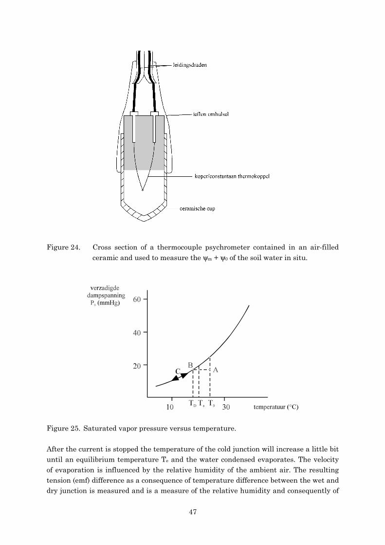
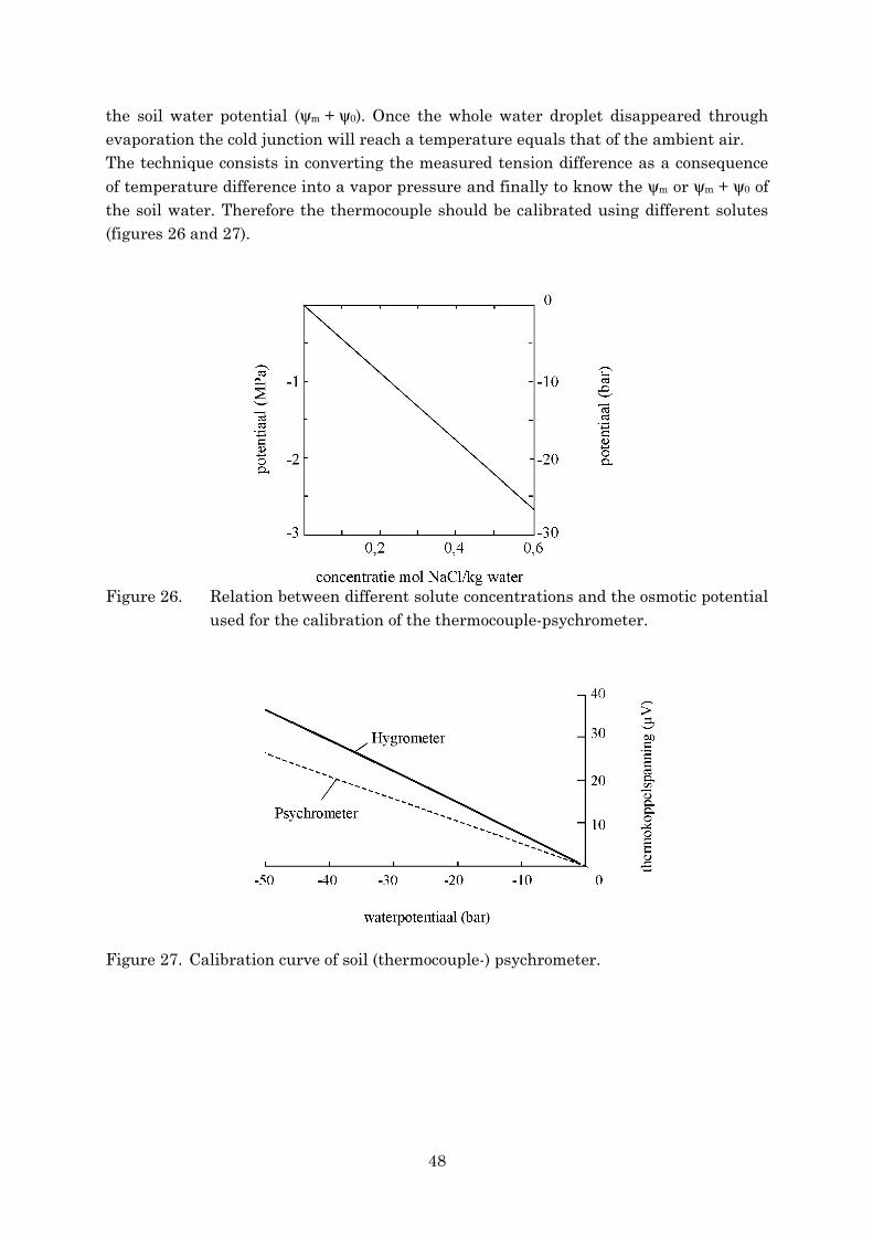
the soil water potential (ψm + ψ0). Once the whole water droplet disappeared throughevaporation the cold junction will reach a temperature equals that of the ambient air.The technique consists in converting the measured tension difference as a consequenceof temperature difference into a vapor pressure and finally to know the ψm or ψm + ψ0 ofthe soil water. Therefore the thermocouple should be calibrated using different solutes(figures 26 and 27).

Figure 26. Relation between different solute concentrations and the osmotic potentialused for the calibration of the thermocouple-psychrometer.

Figure 27. Calibration curve of soil (thermocouple-) psychrometer.

49

3.3. Hysteresis effect.

The relation between matric potential and soil moisture content can be obtained in twoways:- in desorption, by taking an initially saturated sample and applying increasing

pressure to gradually dry the soil while taking successive measurements of moisturecontent versus soil water pressure head or matric potential

- in sorption, by gradually wetting up an initially dry soil sample while reducing thepressure.

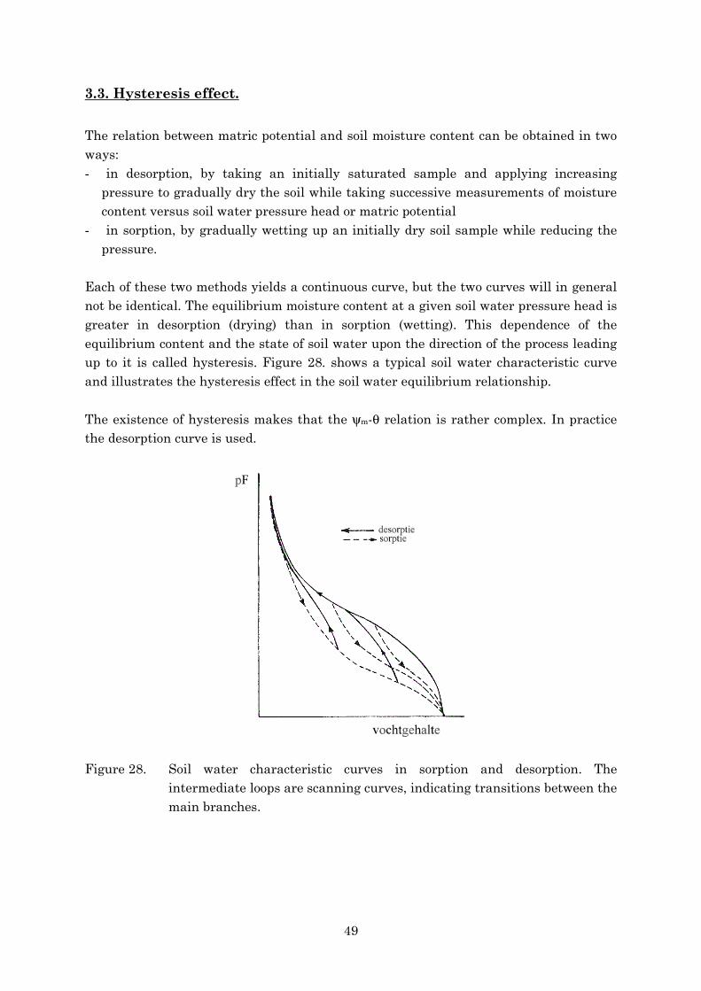
Each of these two methods yields a continuous curve, but the two curves will in generalnot be identical. The equilibrium moisture content at a given soil water pressure head isgreater in desorption (drying) than in sorption (wetting). This dependence of theequilibrium content and the state of soil water upon the direction of the process leadingup to it is called hysteresis. Figure 28. shows a typical soil water characteristic curveand illustrates the hysteresis effect in the soil water equilibrium relationship.

The existence of hysteresis makes that the ψm-θ relation is rather complex. In practicethe desorption curve is used.

Figure 28. Soil water characteristic curves in sorption and desorption. Theintermediate loops are scanning curves, indicating transitions between themain branches.

50

The hysteresis effect may be attributed to several causes:

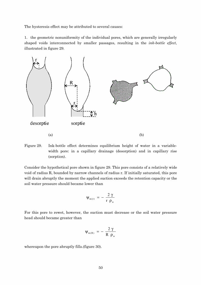
1. the geometric nonuniformity of the individual pores, which are generally irregularlyshaped voids interconnected by smaller passages, resulting in the ink-bottle effect,illustrated in figure 29.

(a) (b)

Figure 29. Ink-bottle effect determines equilibrium height of water in a variable-width pore: in a capillary drainage (desorption) and in capillary rise(sorption).

Consider the hypothetical pore shown in figure 29. This pore consists of a relatively widevoid of radius R, bounded by narrow channels of radius r. If initially saturated, this porewill drain abruptly the moment the applied suction exceeds the retention capacity or thesoil water pressure should became lower than

w)r(m r

2ργ−=ψ

For this pore to rewet, however, the suction must decrease or the soil water pressurehead should became greater than

w)R(m R

2ργ−=ψ

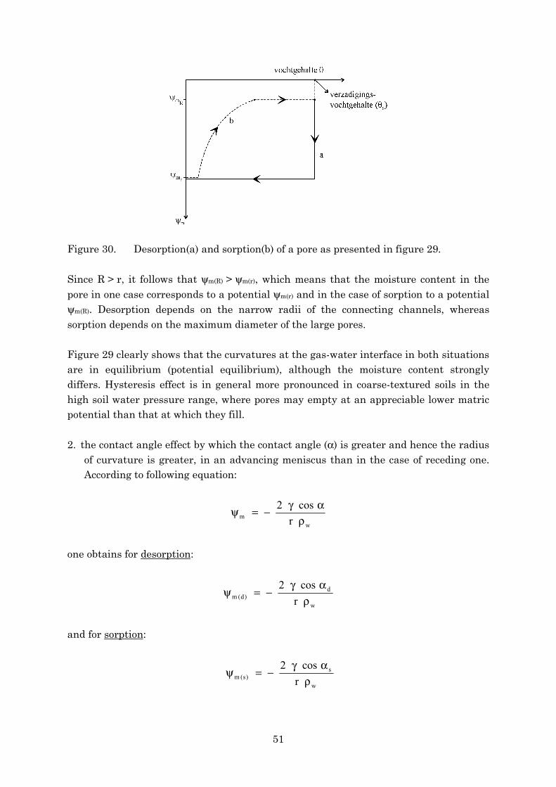
whereupon the pore abruptly fills.(figure 30).

51

Figure 30. Desorption(a) and sorption(b) of a pore as presented in figure 29.

Since R > r, it follows that ψm(R) > ψm(r), which means that the moisture content in thepore in one case corresponds to a potential ψm(r) and in the case of sorption to a potentialψm(R). Desorption depends on the narrow radii of the connecting channels, whereassorption depends on the maximum diameter of the large pores.

Figure 29 clearly shows that the curvatures at the gas-water interface in both situationsare in equilibrium (potential equilibrium), although the moisture content stronglydiffers. Hysteresis effect is in general more pronounced in coarse-textured soils in thehigh soil water pressure range, where pores may empty at an appreciable lower matricpotential than that at which they fill.

2. the contact angle effect by which the contact angle (α) is greater and hence the radiusof curvature is greater, in an advancing meniscus than in the case of receding one.According to following equation:

wm r

cos2ρ

αγ−=ψ

one obtains for desorption:

w

d)d(m r

cos2ρ

αγ−=ψ

and for sorption:

w

s)s(m r

cos2ρ

αγ−=ψ

52

The contact angle is always greater at sorption(α > 0°, cos αs < 1) than at desorption (α =0°, cos αd = 1), due to impurities at the surface of soil particles or the roughness of thesurface so it follows that:

)s(m)d(m ψ⟨ψ

The matric potential ψm(d), whereby the pore with radius r is emptied, is always smallerthan ψm(s), whereby the same pore is filled with water.

3. entrapped air, which further decreases the water content of newly wetted soil.Failure to attain true equilibrium can accentuate the hysteresis effect.

4. swelling and shrinkage phenomena, which result in differential changes of soilstructure, depending on the wetting and drying history of the sample. The gradualsolution of air, or the release of dissolved air from soil water, can also have adifferential effect upon the soil water pressure head – moisture content relationship(pF- curve) in wetting and drying systems.

In the past, hysteresis was generally disregarded in the theory and practice of soilphysics. This may be justifiable in the treatment of processes entailing monotonicwetting (e.g. infiltration) or drying (e.g. evaporation). But the hysteresis effect may beimportant in cases of composite processes in which wetting and drying occursimultaneously or sequentially in various parts of the soil profile (e.g. redistribution). Itis possible to have two soil layers of identical texture and structure at equilibrium witheach other (i.e. at identical energy states) and yet they may differ in wetness or watercontent if their wetting histories have been different. Furthermore, hysteresis can affectthe dynamic, as well as the static, properties of the soil (i.e. hydraulic conductivity andflow phenomena).

The two complete characteristic curves, from saturation to dryness and vice versa, arecalled the main branches of the hysteretic soil moisture characteristic. When a partiallywetted soil commences to drain, or when a partially desorbed soil is rewetted, therelation of soil water pressure head to moisture content follow some intermediate curveas it moves from one branch to the other. Such intermediate spurs are called scanningcurves. Cyclic changes often entail wetting and drying scanning curves, which may formloops between the main branches (figure 28). The h-θ relationship can thus become verycomplicated. Because of its complexity, the hysteresis phenomenon is too often ignored,and the soil water characteristic curve, which is generally reported, is the desorptioncurve, also known as the soil water release curve. The sorption curve, which is equallyimportant but more difficult to determine, is seldom even attempted.

53

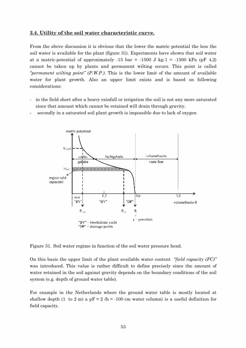
3.4. Utility of the soil water characteristic curve.

From the above discussion it is obvious that the lower the matric potential the less thesoil water is available for the plant (figure 31). Experiments have shown that soil waterat a matric-potential of approximately -15 bar = -1500 J kg-1 = -1500 kPa (pF 4,2)cannot be taken up by plants and permanent wilting occurs. This point is called“permanent wilting point” (P.W.P.). This is the lower limit of the amount of availablewater for plant growth. Also an upper limit exists and is based on followingconsiderations:

- in the field short after a heavy rainfall or irrigation the soil is not any more saturatedsince that amount which cannot be retained will drain through gravity.

- secondly in a saturated soil plant growth is impossible due to lack of oxygen

Figure 31. Soil water regime in function of the soil water pressure head.

On this basis the upper limit of the plant available water content “field capacity (FC)”was introduced. This value is rather difficult to define precisely since the amount ofwater retained in the soil against gravity depends on the boundary conditions of the soilsystem (e.g. depth of ground water table).

For example in the Netherlands where the ground water table is mostly located atshallow depth (1 to 2 m) a pF = 2 (h = -100 cm water column) is a useful definition forfield capacity.

54

For loamy soils in Belgium, where the ground water table is located at great depths, itwas found that the moisture content at -1/3 bar (pF ≈ 2,54) is a useful definition for fieldcapacity, while in sandy soils the moisture content at -0,1 bar (≈ pF 2) reflects thereality.

When a shallow ground water table is present the matric potential at equilibriumfollowing desorption and corresponding to the definition of field capacity is equal to thenegative value of of the distance from the point under consideration to the depth of theground water table.

This discussion shows that field capacity is only a useful definition for a specificsituation in the field. It is generally defined as the amount of water, which remained inthe soil 2 or 3 days after a heavy rain and whereby evaporation was avoided. Thepresumed water content at which internal drainage allegedly ceases, termed the fieldcapacity, had for a long time been accepted almost universally as an actual physicalproperty, characteristic of a constant for each soil. However the term field capacityconcept may have done more harm than good since when and how can one determinethat the redistribution has virtually ceased, or that its rate has become negligible orpractically zero.

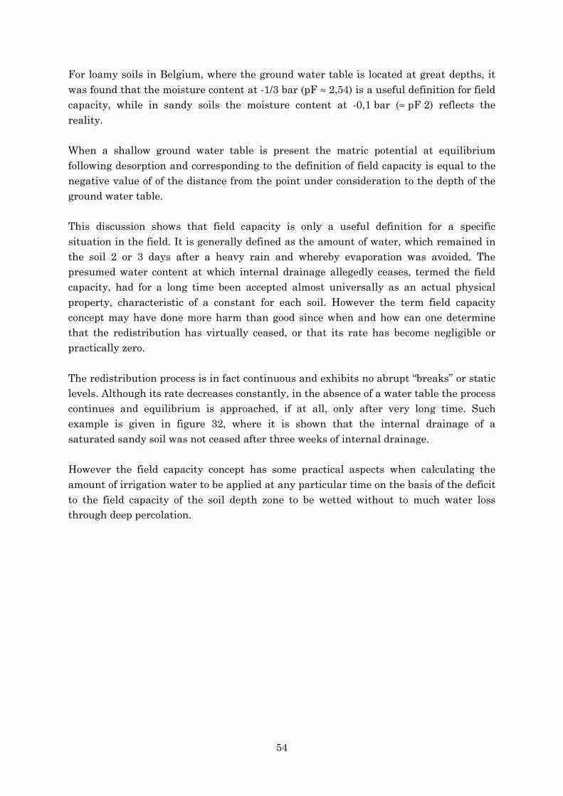
The redistribution process is in fact continuous and exhibits no abrupt “breaks” or staticlevels. Although its rate decreases constantly, in the absence of a water table the processcontinues and equilibrium is approached, if at all, only after very long time. Suchexample is given in figure 32, where it is shown that the internal drainage of asaturated sandy soil was not ceased after three weeks of internal drainage.

However the field capacity concept has some practical aspects when calculating theamount of irrigation water to be applied at any particular time on the basis of the deficitto the field capacity of the soil depth zone to be wetted without to much water lossthrough deep percolation.

55

Figure 32. Change of moisture content in function of time during an internaldrainage in a sandy soil and whereby evaporation was avoided.

The moisture content/matric potential of a soil has to be estimated in the field.Therefore a plot, where tensiometers are installed at different depths, is saturated,followed by an internal drainage, whereby evaporation has to be avoided. During theinternal drainage the soil water pressure head is measured at regular times. After somedays the rate of decrease is strongly reduced and a “quasi” equilibrium is reached andthe matric potential at that time is taken as the matric potential at field capacity.Simultaneous soil sampling will allow the estimation of the corresponding moisturecontent.

Where the moisture content at P.W.P. is determined by the composition of the soil(texture and organic matter) the moisture content at F.C. is function of its composition,soil structure and field situation as well.

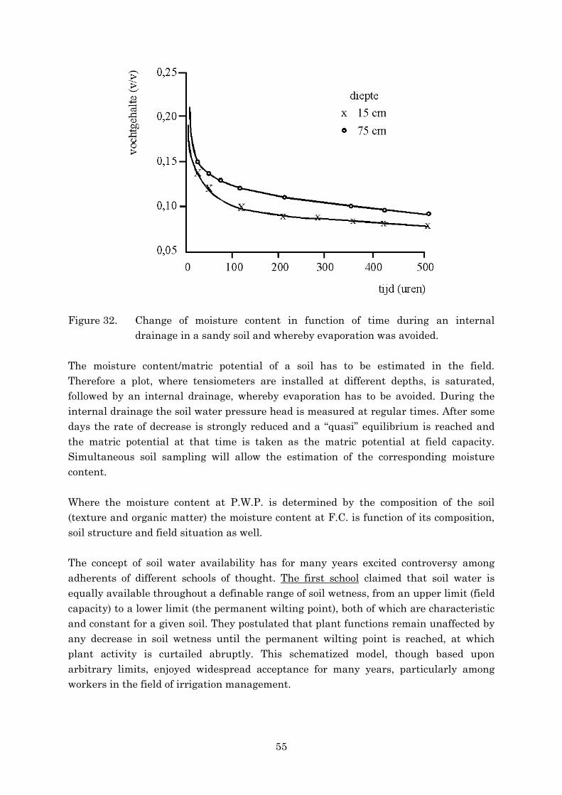
The concept of soil water availability has for many years excited controversy amongadherents of different schools of thought. The first school claimed that soil water isequally available throughout a definable range of soil wetness, from an upper limit (fieldcapacity) to a lower limit (the permanent wilting point), both of which are characteristicand constant for a given soil. They postulated that plant functions remain unaffected byany decrease in soil wetness until the permanent wilting point is reached, at whichplant activity is curtailed abruptly. This schematized model, though based uponarbitrary limits, enjoyed widespread acceptance for many years, particularly amongworkers in the field of irrigation management.

56

A second school however produced evidence indicating that soil water availability toplants actually decreases with decreasing soil wetness, and that a plant may sufferwater stress and reduction of growth considerably before the wilting point is reached.

A third school seeking to compromise between the opposing views, attempted to dividethe so-called available ranges, and searched for a critical point somewhere between fieldcapacity and wilting point as an additional criterion of soil water availability.

These different hypotheses are represented graphically in figure 33.

Figure 33. Three classical hypotheses regarding the availability of soil water toplantsa. equal availability from field capacity to wilting pointb. equal availability from field capacity to a critical moisture content

beyond which availability decreasesc. availability decreases gradually as soil moisture content decreases

None of these school was able up to now to base its hypotheses upon a comprehensiveframework that could take into account the array of factors likely to influence the waterregime of the soil-water-atmosphere system as a whole.

Since it was recognized that soil wetness per se is not a satisfactory criterion foravailability, attempts were made to correlate the water status of plants with the energystate of soil water, i.e. with the soil water potential. The soil water constants weretherefore defined in terms of potential values, which could be applied universally, ratherthan in terms of soil wetness.

The availability of soil water is not only determined by the matric potential but alsoinfluenced by the osmotic potential of the soil water. Assume a soil with a ψm = -300 cm WH and a ψ0 = -14500 cm WH – due to the presence of salts – than the sum ofboth potentials, also called the water potential ψw , is so low that wilting will occur. Dueto the presence of solutes the "ψw-θ"-curve (pψw-curve, in analogy with the pF-curve) is

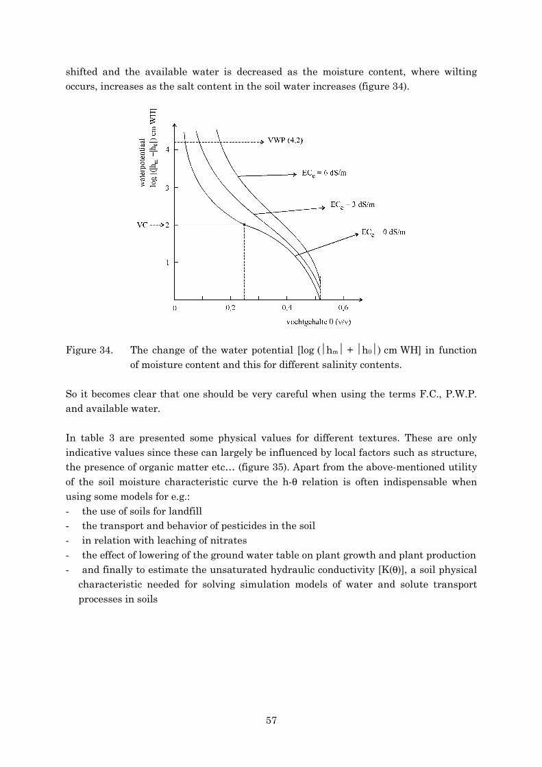
57

shifted and the available water is decreased as the moisture content, where wiltingoccurs, increases as the salt content in the soil water increases (figure 34).

Figure 34. The change of the water potential [log (hm + h0) cm WH] in functionof moisture content and this for different salinity contents.

So it becomes clear that one should be very careful when using the terms F.C., P.W.P.and available water.

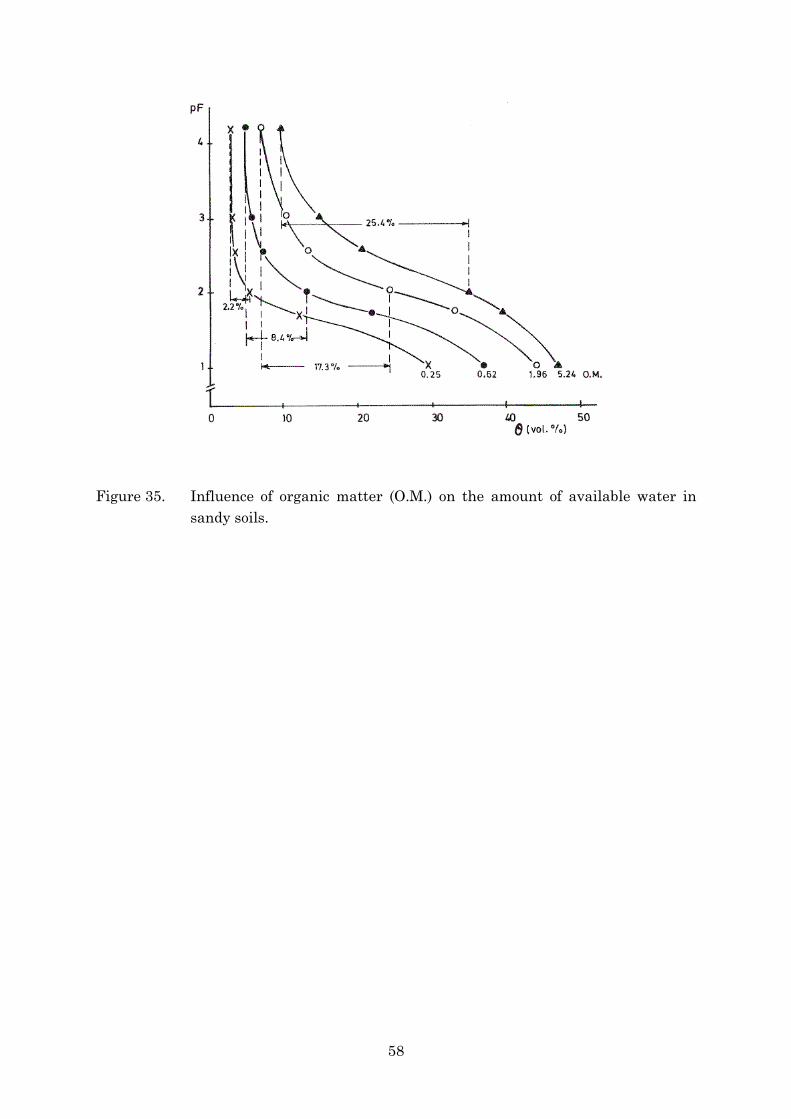
In table 3 are presented some physical values for different textures. These are onlyindicative values since these can largely be influenced by local factors such as structure,the presence of organic matter etc… (figure 35). Apart from the above-mentioned utilityof the soil moisture characteristic curve the h-θ relation is often indispensable whenusing some models for e.g.:- the use of soils for landfill- the transport and behavior of pesticides in the soil- in relation with leaching of nitrates- the effect of lowering of the ground water table on plant growth and plant production- and finally to estimate the unsaturated hydraulic conductivity [K(θ)], a soil physical

characteristic needed for solving simulation models of water and solute transportprocesses in soils

58

Figure 35. Influence of organic matter (O.M.) on the amount of available water insandy soils.

59

59

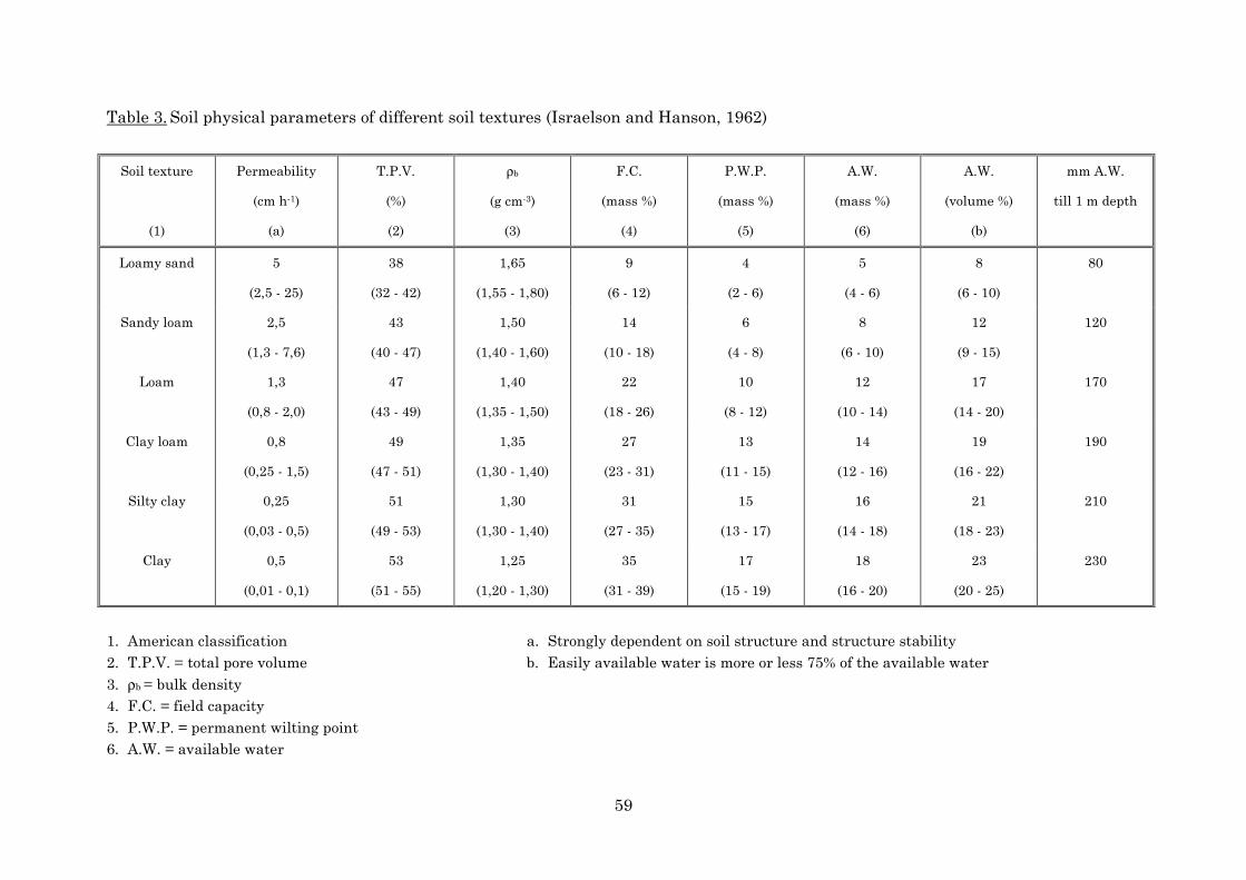
Table 3. Soil physical parameters of different soil textures (Israelson and Hanson, 1962)

Soil texture

(1)

Permeability

(cm h-1)

(a)

T.P.V.

(%)

(2)

ρb

(g cm-3)

(3)

F.C.

(mass %)

(4)

P.W.P.

(mass %)

(5)

A.W.

(mass %)

(6)

A.W.

(volume %)

(b)

mm A.W.

till 1 m depth

Loamy sand 5

(2,5 - 25)

38

(32 - 42)

1,65

(1,55 - 1,80)

9

(6 - 12)

4

(2 - 6)

5

(4 - 6)

8

(6 - 10)

80

Sandy loam 2,5

(1,3 - 7,6)

43

(40 - 47)

1,50

(1,40 - 1,60)

14

(10 - 18)

6

(4 - 8)

8

(6 - 10)

12

(9 - 15)

120

Loam 1,3

(0,8 - 2,0)

47

(43 - 49)

1,40

(1,35 - 1,50)

22

(18 - 26)

10

(8 - 12)

12

(10 - 14)

17

(14 - 20)

170

Clay loam 0,8

(0,25 - 1,5)

49

(47 - 51)

1,35

(1,30 - 1,40)

27

(23 - 31)

13

(11 - 15)

14

(12 - 16)

19

(16 - 22)

190

Silty clay 0,25

(0,03 - 0,5)

51

(49 - 53)

1,30

(1,30 - 1,40)

31

(27 - 35)

15

(13 - 17)

16

(14 - 18)

21

(18 - 23)

210

Clay 0,5

(0,01 - 0,1)

53

(51 - 55)

1,25

(1,20 - 1,30)

35

(31 - 39)

17

(15 - 19)

18

(16 - 20)

23

(20 - 25)

230

1. American classification a. Strongly dependent on soil structure and structure stability2. T.P.V. = total pore volume b. Easily available water is more or less 75% of the available water3. ρb = bulk density4. F.C. = field capacity5. P.W.P. = permanent wilting point6. A.W. = available water

33