III Smith VNA Improved2 - uniroma1.itarpg-serv.ing2.uniroma1.it/.../III_Smith_VNA_Improved.pdf · 6...

1

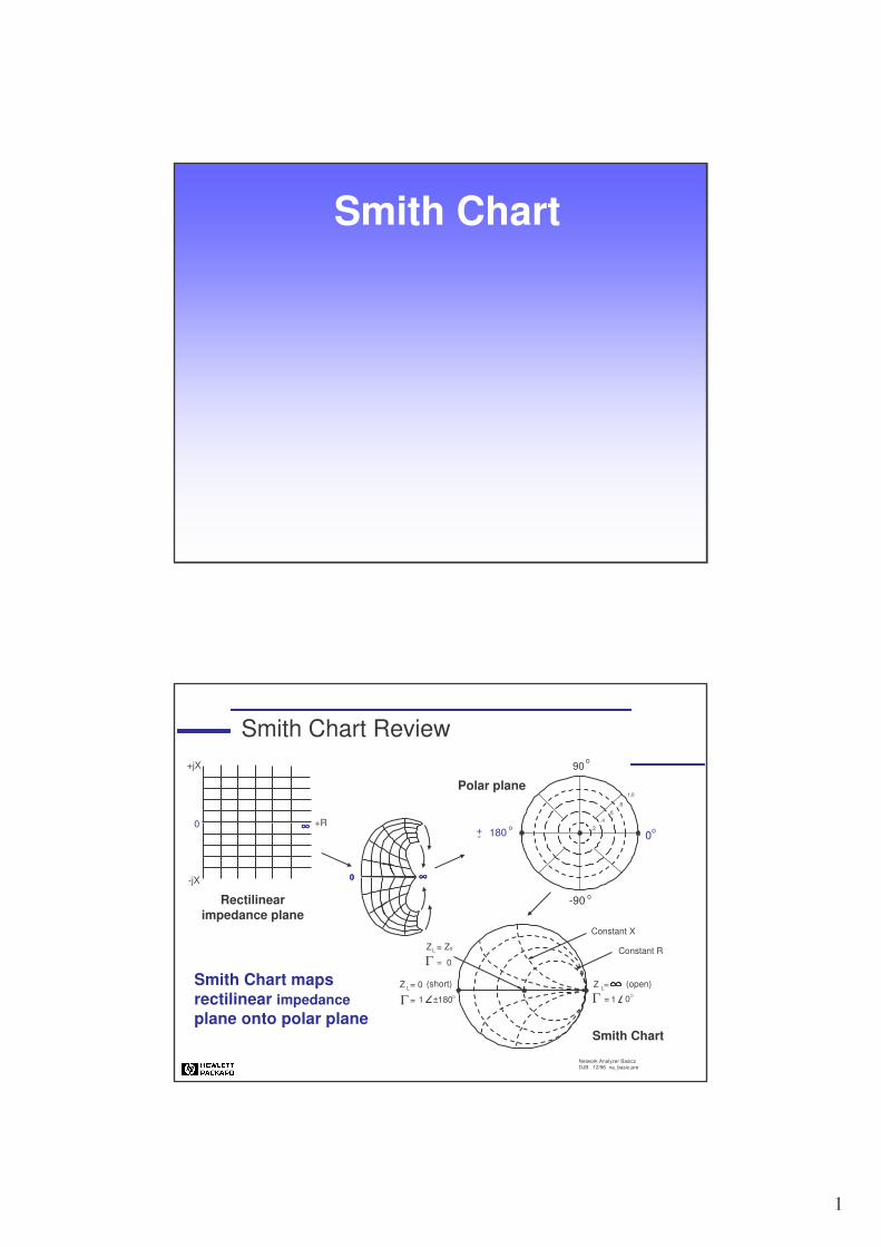
Smith Chart

Network Analyzer BasicsDJB 12/96 na_basic.pre

Smith Chart Review.

-90 o

0o180 o+-.2

.4

.6

.8

1.0

90o

∞∞∞∞0000

0 +R

+jX

-jX

∞∞∞∞

Smith Chart maps rectilinear impedanceplane onto polar plane

Rectilinear impedance plane

Polar plane

Z = ZoL

= 0Γ

Constant X

Constant R

Z = L

= 0 O1Γ

Smith Chart

(open)

ΓLZ = 0

= ±180 O1

(short)

2

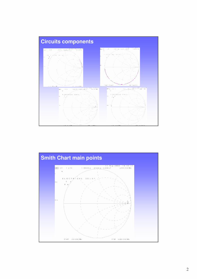
Circuits components

Smith Chart main points

3

From S parameters to impedance

IF BW and averaging

Heterodyne detection scheme

IF BW reduction

Averaging

Dynamic Range (definition)

4

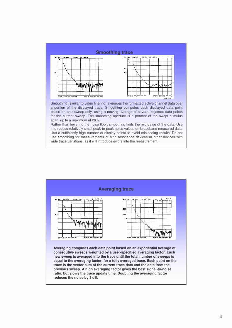
Smoothing trace

Smoothing (similar to video filtering) averages the formatted active channel data over a portion of the displayed trace. Smoothing computes each displayed data point based on one sweep only, using a moving average of several adjacent data points for the current sweep. The smoothing aperture is a percent of the swept stimulus span, up to a maximum of 20%.Rather than lowering the noise floor, smoothing finds the mid-value of the data. Use it to reduce relatively small peak-to-peak noise values on broadband measured data. Use a sufficiently high number of display points to avoid misleading results. Do not use smoothing for measurements of high resonance devices or other devices with wide trace variations, as it will introduce errors into the measurement.

Averaging trace

Averaging computes each data point based on an exponential average of consecutive sweeps weighted by a user-specified averaging factor. Each new sweep is averaged into the trace until the total number of sweeps is equal to the averaging factor, for a fully averaged trace. Each point on the trace is the vector sum of the current trace data and the data from the previous sweep. A high averaging factor gives the best signal-to-noise ratio, but slows the trace update time. Doubling the averaging factor reduces the noise by 3 dB.

5

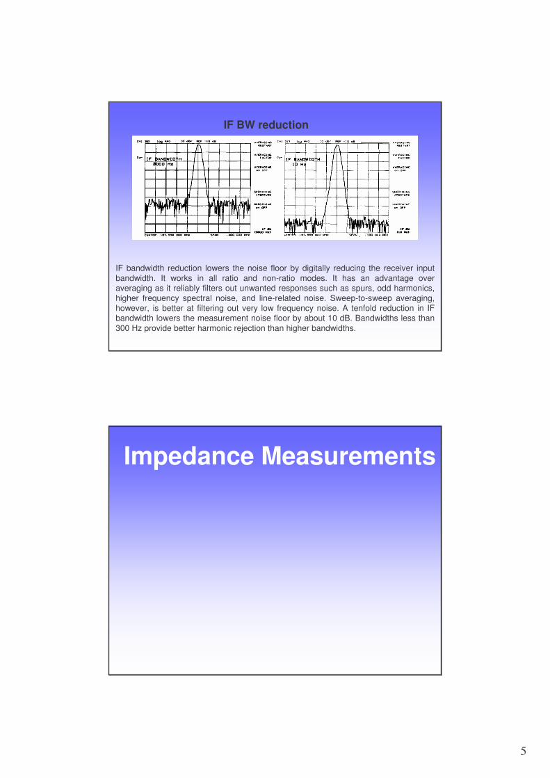
IF BW reduction

IF bandwidth reduction lowers the noise floor by digitally reducing the receiver input bandwidth. It works in all ratio and non-ratio modes. It has an advantage over averaging as it reliably filters out unwanted responses such as spurs, odd harmonics, higher frequency spectral noise, and line-related noise. Sweep-to-sweep averaging, however, is better at filtering out very low frequency noise. A tenfold reduction in IF bandwidth lowers the measurement noise floor by about 10 dB. Bandwidths less than 300 Hz provide better harmonic rejection than higher bandwidths.

Impedance Measurements

6

H Kobe Instrument DivisionBack to Basics - LCRZ Module

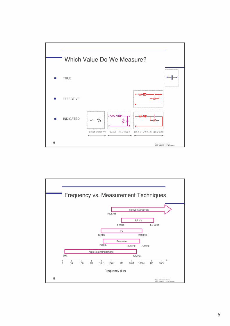
Which Value Do We Measure?

TRUE

EFFECTIVE

INDICATED +/-

Instrument Test fixture Real world device

%


Frequency vs. Measurement Techniques

Network Analysis

100KHz

1 10 100 1K 10K 100K 1M 10M 100M 1G 10G

Frequency (Hz)

Auto Balancing Bridge5HZ 40MHz

22KHz 70MHz

Resonant

I-V10KHz 110MHz

30MHz

RF I-V

1 MHz 1.8 GHz

7


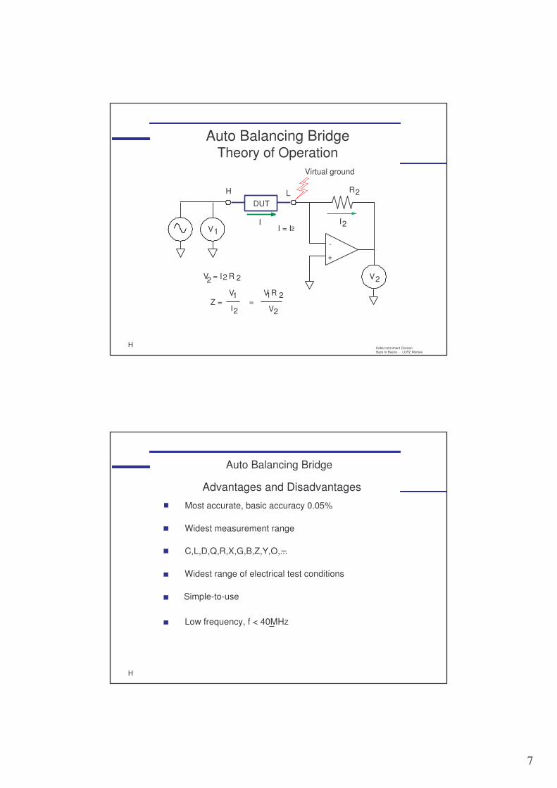
Auto Balancing BridgeTheory of Operation

V

-

+

2

V1

DUT

V = I R2 2 2

Z = V

I

1

2=

V R

V

21

2

H L R2

I2

Virtual ground

II = I2

H

Auto Balancing Bridge

Most accurate, basic accuracy 0.05%

Widest measurement range

Widest range of electrical test conditions

Simple-to-use

Advantages and Disadvantages

Low frequency, f < 40MHz

C,L,D,Q,R,X,G,B,Z,Y,O,...

8


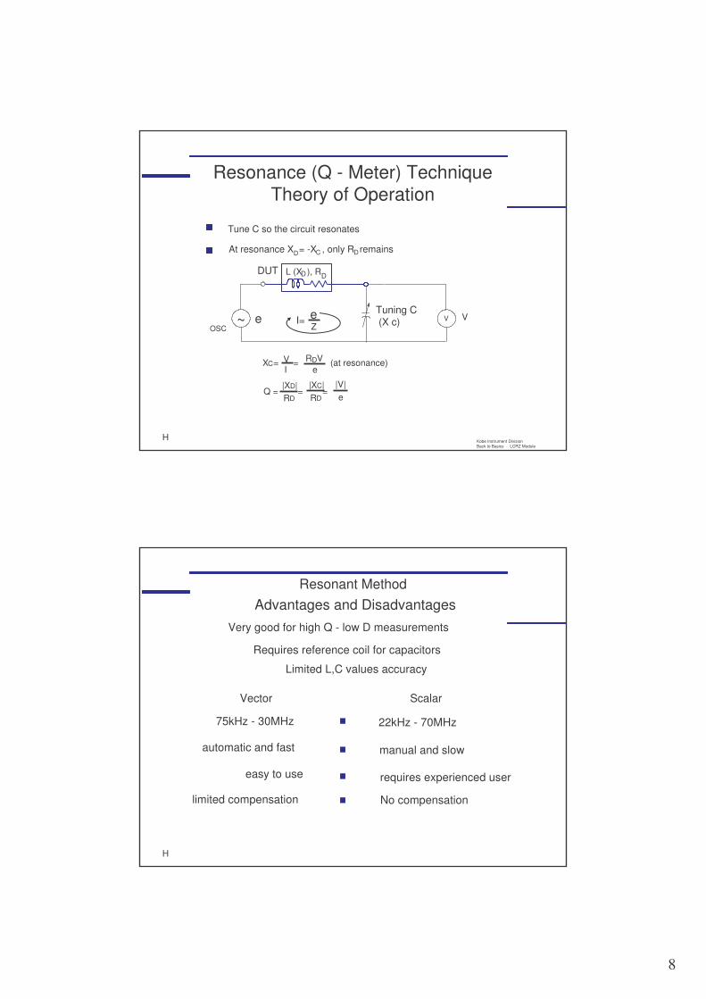
Resonance (Q - Meter) TechniqueTheory of Operation

Tune C so the circuit resonates

At resonance X = -X , only R remainsD C D

V~OSC

Tuning C(X c) V

L (X ), RD DDUT

e I= eZ

X = = (at resonance)C VI

R VeD

Q = = =|V|e

|X |RD

D |X |RD

C

H

Resonant MethodAdvantages and Disadvantages

requires experienced user

Vector Scalar

automatic and fast manual and slow

easy to use

No compensationlimited compensation

75kHz - 30MHz 22kHz - 70MHz

Very good for high Q - low D measurements

Requires reference coil for capacitors

Limited L,C values accuracy

9


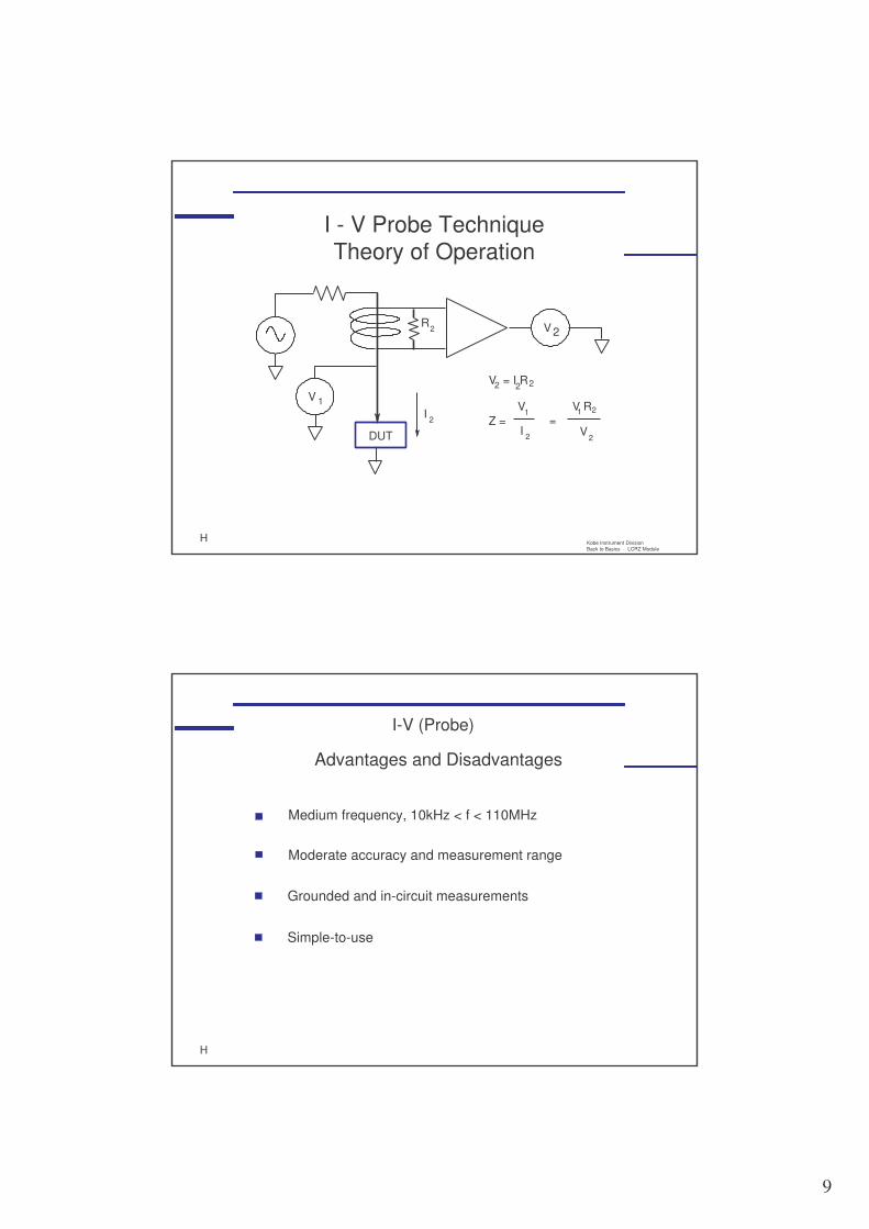
I - V Probe TechniqueTheory of Operation

V2

V 1

DUT

V = I R2 2 2

Z = V

I

1

2

= V R

V

21

2

I 2

R2

H

I-V (Probe)

Medium frequency, 10kHz < f < 110MHz

Moderate accuracy and measurement range


Grounded and in-circuit measurements

Simple-to-use

10


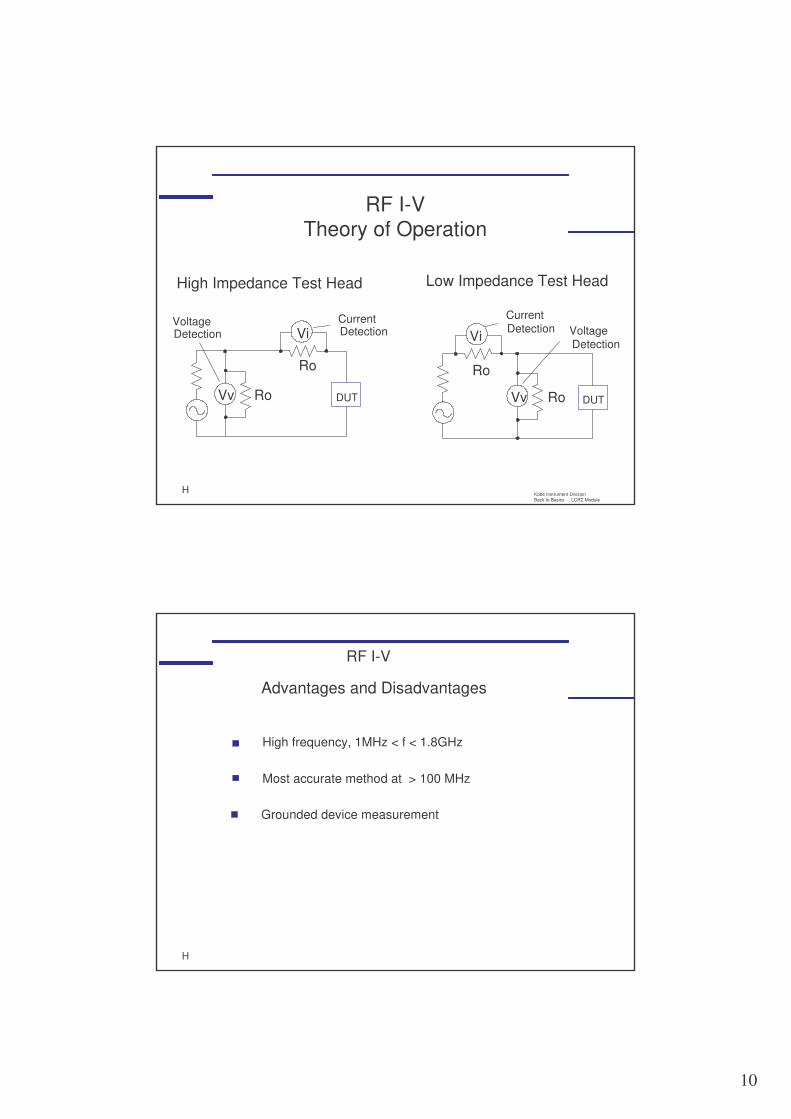
RF I-VTheory of Operation

Vi

Vv

Ro

Ro

Vi

Vv

Ro

Ro DUT DUT

Voltage CurrentVoltageDetection Detection

CurrentDetection

Detection

High Impedance Test Head Low Impedance Test Head

H

RF I-V

High frequency, 1MHz < f < 1.8GHz

Most accurate method at > 100 MHz

Grounded device measurement


11


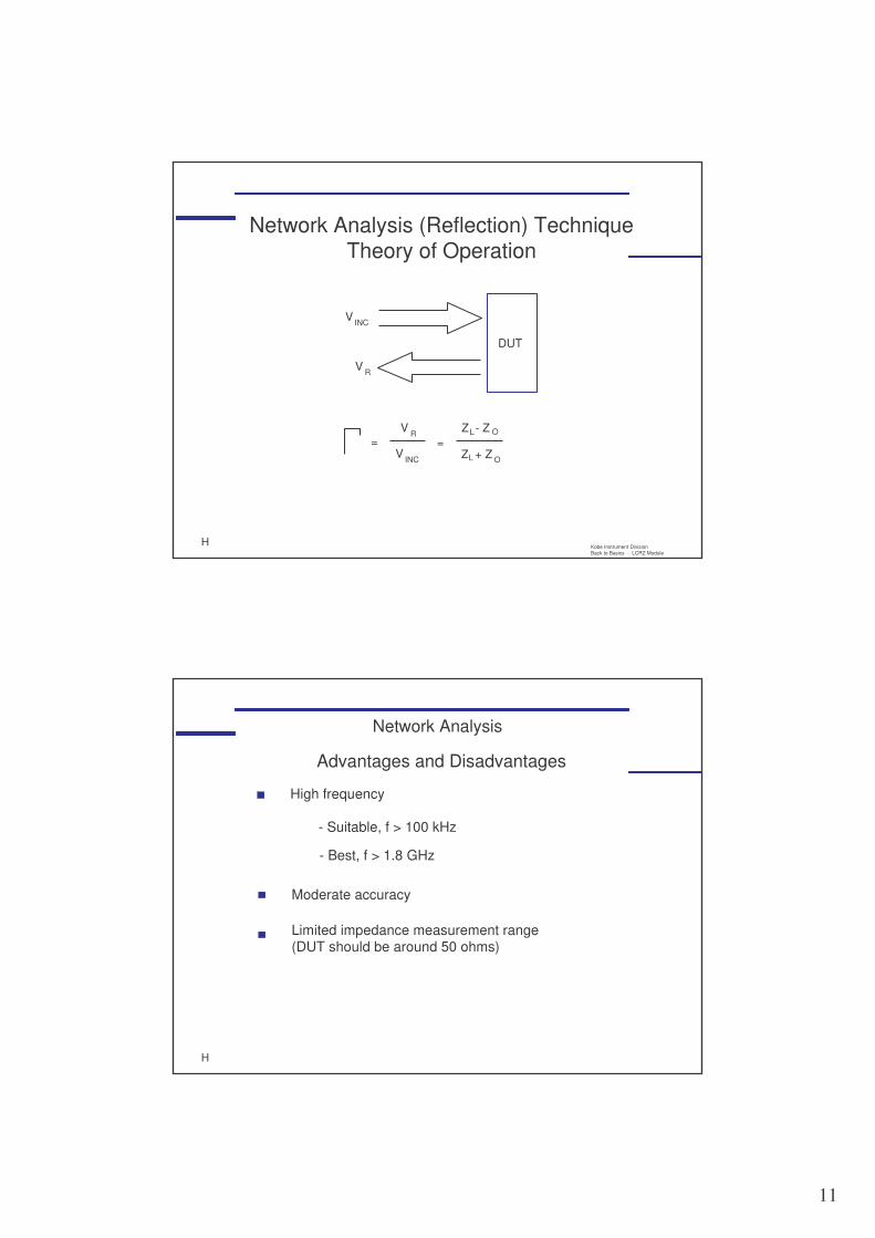
Network Analysis (Reflection) TechniqueTheory of Operation

DUT

V

V INC

R

V

V INC

R Z - ZL O

Z + ZL O

==

H

Network Analysis

High frequency

- Suitable, f > 100 kHz

Moderate accuracy

Limited impedance measurement range(DUT should be around 50 ohms)


- Best, f > 1.8 GHz

12

H Kobe Instrument DivisionBack to Basics - LCRZ ModuleH

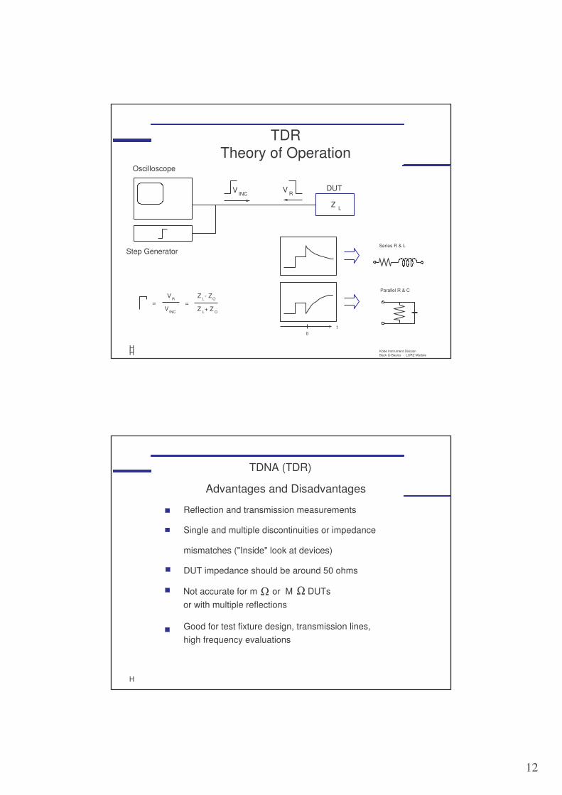
TDRTheory of Operation

V

V INC

RZ - ZL O

Z + ZL O

==

Z L

DUT

Oscilloscope

Step Generator

VV INC R

Series R & L

Parallel R & C

0t

H

TDNA (TDR)

Reflection and transmission measurements

Single and multiple discontinuities or impedance


DUT impedance should be around 50 ohms

mismatches ("Inside" look at devices)

Good for test fixture design, transmission lines,high frequency evaluations

ΩNot accurate for m or M DUTsor with multiple reflections

Ω

13

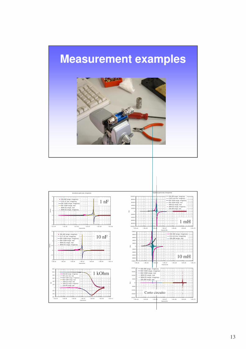
Measurement examples

Ammettenza (parte reale, immaginaria)

-2

-1

0

1

2

3

4

1.0E+04 1.0E+05 1.0E+06 1.0E+07 1.0E+08 1.0E+09frequenza (Hz)

Sie

men

s

30k-6M range, imaginary0.92 nF line, imaginary5M-100M range, imaginary5M-100M range, real80M-2G range, real80M-2G range, imaginary

-5

-2.5

0

2.5

5

7.5

10

1.0E+04 1.0E+05 1.0E+06 1.0E+07 1.0E+08 1.0E+09 1.0E+10frequenza (Hz)

Sie

men

s

30k-6M range, imaginary9.27 nF line, imaginary5M-100M range, imaginary5M-100M range, real80M-2G range, real80M-2G range, imaginary

-600

-400

-200

0

200

400

600

800

1000

1200


Oh

m

30k-6M range, imaginary991 ohm line, real5M-100M range, imaginary5M-100M range, real80M-2G range, real80M-2G range, imaginary30k-6M range, real

Impedenza (parte reale, immaginaria)

-100000

-80000

-60000

-40000

-20000

0

20000

40000

60000

80000

100000


Ohm

30k-6M range, imaginary0.972 mH line, imaginary5M-100M range, imaginary5M-100M range, real80M-2G range, real80M-2G range, imaginary30k-6M range, real

-100000

-80000

-60000

-40000

-20000

0

20000

40000

60000

80000

100000


Ohm

30k-6M range, imaginary8.6 mH line, imaginary30k-6M range, real

-20000

-15000

-10000

-5000

0

5000

10000

15000

20000


Ohm

30k-6M range, imaginary5M-100M range, imaginary5M-100M range, real80M-2G range, real80M-2G range, imaginary30k-6M range, real

1 nF

10 nF

10 mH

1 mH

Corto circuito

1 kOhm

14

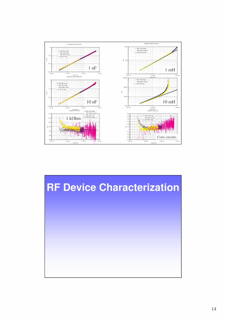
Ammettenza (parte immaginaria)

0.0001

0.001

0.01

0.1

1.0E+04 1.0E+05 1.0E+06 1.0E+07frequenza (Hz)

Sie

men

s

30k-6M range30k-1M range30k-600k range0.92 nF line

Ammettenza (parte immaginaria)

0.001

0.01

0.1

1


Sie

men

s

30k-6M range30k-1M range30k-600k range9.27 nF line

Impedenza (parte reale)

980

985

990

995

1000

1005

1010


Ohm

30k-1M range30k-600k range991 Ohm line30k-6M range

Impedenza (parte immaginaria)

100

1000

10000

1.0E+04 1.0E+05 1.0E+06frequenza (Hz)

Oh

m

30k-1M range30k-600k range0.972 mH line

1000

10000

100000

1000000

1.0E+04 1.0E+05 1.0E+06frequenza (Hz)

Ohm

30k-1M range30k-600k range8.6 mH line

Impedenza (parte reale)

-0.04

-0.03

-0.02

-0.01

0

0.01

0.02

0.03

0.04

0.05

0.06


Oh

m

30k-1M range30k-600k range30k-6M range

1 nF

10 nF 10 mH

1 mH

Corto circuito

1 kOhm

RF Device Characterization

15

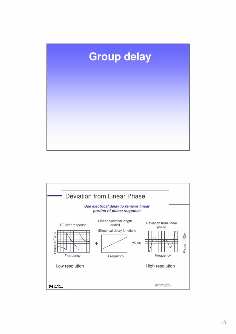
Group delay


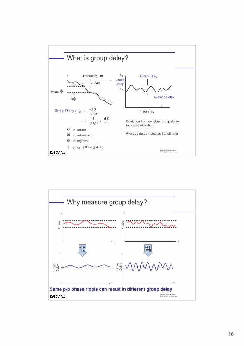
Deviation from Linear PhaseUse electrical delay to remove linear

portion of phase response

Linear electrical length added

+ yields

Frequency

(Electrical delay function)

Frequency

RF filter response Deviation from linear phase

Pha

se 1

/D

ivo

Pha

se 4

5 /D

ivo

Frequency

Low resolution High resolution

16


What is group delay?

Deviation from constant group delay indicates distortion

Average delay indicates transit time

Frequency

Group DelayGroupDelay

Average Delay

Phaset o

t g

Group Delay (t )g

=−1360 o

= −d φd ω

d φd f

in radians

in radians/sec

in degrees

in Hzf

φωφ

2=( )fω π

φ

∆φ

Frequency

*

∆ω

ω


Why measure group delay?

Same p-p phase ripple can result in different group delay

Pha

se

Pha

se

Gro

up

Del

ay

Gro

up

Del

ay

−−−−d φφφφd ωωωω

−−−−d φφφφd ωωωω

f

f

f

f

III Smith VNA Improved2 - uniroma1.itarpg-serv.ing2.uniroma1.it/.../III_Smith_VNA_Improved.pdf · 6...

Documents

Transcript of III Smith VNA Improved2 - uniroma1.itarpg-serv.ing2.uniroma1.it/.../III_Smith_VNA_Improved.pdf · 6...