Heisenberg uniqueness pairs and the Klein-Gordon equation
21
Annals of Mathematics 173 (2011), 1507–1527 doi: 10.4007/annals.2011.173.3.6 Heisenberg uniqueness pairs and the Klein-Gordon equation By Haakan Hedenmalm and Alfonso Montes-Rodr´ ıguez Abstract A Heisenberg uniqueness pair (HUP) is a pair (Γ, Λ), where Γ is a curve in the plane and Λ is a set in the plane, with the following property: any finite Borel measure μ in the plane supported on Γ, which is absolutely continuous with respect to arc length, and whose Fourier transform b μ van- ishes on Λ, must automatically be the zero measure. We prove that when Γ is the hyperbola x1x2 = 1 and Λ is the lattice-cross Λ=(αZ ×{0}) ∪ ({0}× βZ), where α, β are positive reals, then (Γ, Λ) is an HUP if and only if αβ ≤ 1; in this situation, the Fourier transform b μ of the measure solves the one- dimensional Klein-Gordon equation. Phrased differently, we show that e πiαnt , e πiβn/t , n ∈ Z, span a weak-star dense subspace in L ∞ (R) if and only if αβ ≤ 1. In order to prove this theorem, some elements of linear fractional theory and ergodic theory are needed, such as the Birkhoff Ergodic Theorem. An idea parallel to the one exploited by Makarov and Poltoratski (in the context of model subspaces) is also needed. As a consequence, we solve a problem on the density of algebras generated by two inner functions raised by Matheson and Stessin. 1. Introduction Heisenberg uniqueness pairs. Let μ be a finite complex-valued Borel mea- sure in the plane R 2 . Associate to it the Fourier transform b μ(ξ )= Z R 2 e πihx,ξi dμ(x), where x =(x 1 ,x 2 ) and ξ =(ξ 1 ,ξ 2 ), with inner product hx, ξ i = x 1 ξ 1 + x 2 ξ 2 . The research of the first named author was partially supported by the G¨ oran Gustafsson Foundation (KVA) and by Vetenskapsr˚ adet (VR). The research of the second named author was partially supported by Plan Nacional I+D+I grant no. MTM2009-09501 and by Junta de Andaluc´ ıa grants nos. FQM-260 and FQM06-02225. El trabajo de Alfonso Montes-Rodr´ ıguez est´ a dedicado a su hijo Alfonso Montes Reina que falleci´o el 1 de junio de 2009. 1507
Transcript of Heisenberg uniqueness pairs and the Klein-Gordon equation
Annals of Mathematics 173 (2011), 1507–1527doi: 10.4007/annals.2011.173.3.6
Heisenberg uniqueness pairs andthe Klein-Gordon equation
By Haakan Hedenmalm and Alfonso Montes-Rodrıguez
Abstract
A Heisenberg uniqueness pair (HUP) is a pair (Γ,Λ), where Γ is a curve
in the plane and Λ is a set in the plane, with the following property: any
finite Borel measure µ in the plane supported on Γ, which is absolutely
continuous with respect to arc length, and whose Fourier transform µ van-
ishes on Λ, must automatically be the zero measure. We prove that when
Γ is the hyperbola x1x2 = 1 and Λ is the lattice-cross
Λ = (αZ× {0}) ∪ ({0} × βZ),
where α, β are positive reals, then (Γ,Λ) is an HUP if and only if αβ ≤ 1;
in this situation, the Fourier transform µ of the measure solves the one-
dimensional Klein-Gordon equation. Phrased differently, we show that
eπiαnt, eπiβn/t, n ∈ Z,
span a weak-star dense subspace in L∞(R) if and only if αβ ≤ 1. In order
to prove this theorem, some elements of linear fractional theory and ergodic
theory are needed, such as the Birkhoff Ergodic Theorem. An idea parallel
to the one exploited by Makarov and Poltoratski (in the context of model
subspaces) is also needed. As a consequence, we solve a problem on the
density of algebras generated by two inner functions raised by Matheson
and Stessin.
1. Introduction
Heisenberg uniqueness pairs. Let µ be a finite complex-valued Borel mea-
sure in the plane R2. Associate to it the Fourier transform
µ(ξ) =
∫R2
eπi〈x,ξ〉dµ(x),
where x = (x1, x2) and ξ = (ξ1, ξ2), with inner product
〈x, ξ〉 = x1ξ1 + x2ξ2.
The research of the first named author was partially supported by the Goran Gustafsson
Foundation (KVA) and by Vetenskapsradet (VR). The research of the second named author
was partially supported by Plan Nacional I+D+I grant no. MTM2009-09501 and by Junta
de Andalucıa grants nos. FQM-260 and FQM06-02225.
El trabajo de Alfonso Montes-Rodrıguez esta dedicado a su hijo Alfonso Montes Reina
que fallecio el 1 de junio de 2009.
1507
1508 HAAKAN HEDENMALM and ALFONSO MONTES-RODRIGUEZ
The Heisenberg uncertainty principle states that µ and µ cannot both be too
concentrated to a point (see [6] for the original paper of Heisenberg, and [5]
for a more general treatment); in particular, they cannot both have compact
support (unless µ = 0). Here, we shall study a variation on that theme. Let Γ
be a smooth curve in R2, or, more generally, a finite disjoint union of smooth
curves. Suppose that suppµ ⊂ Γ and that µ is absolutely continuous with
respect to arc length measure on Γ. Which sets Λ ⊂ R2 have the property that
µ|Λ = 0 =⇒ µ = 0?
If this is the case, we say that (Γ,Λ) is a Heisenberg uniqueness pair. A dual
formulation is that (Γ,Λ) is a Heisenberg uniqueness pair if and only if the
functionseξ(x) = eπi〈x,ξ〉, ξ ∈ Λ
span a weak-star dense subspace in L∞(Γ). This concept of Heisenberg unique-
ness pairs has many features in common with the notion of (weakly) mutually
annihilating pairs of Borel measurable sets having positive area measure, which
appears, for instance, in the book by Havin and Joricke [5].
The properties of the Fourier transform with respect to translation and
multiplication by complex exponentials show that for all points x∗, ξ∗ ∈ R2,
we have
(inv-1) (Γ + {x∗},Λ + {ξ∗}) is an HUP ⇐⇒ (Γ,Λ) is an HUP,
where HUP is short for “Heisenberg uniqueness pair”. Likewise, it is also
straightforward to see that if T : R2 → R2 is an invertible linear transformation
with adjoint T ∗, then
(inv-2) (T−1(Γ), T ∗(Λ)) is an HUP ⇐⇒ (Γ,Λ) is an HUP.
Algebraic curves and partial differential equations. Algebraic curves Γ are
of particular interest because of their connection to partial differential equa-
tions. That connection follows from the observation that for polynomials p of
two variables,
p
Ç∂1
πi,∂2
πi
åµ(ξ) =
∫R2
eπi〈x,ξ〉 p(x1, x2) dµ(x),
so that if p is real-valued and Γ is the locus of the equation
p(x1, x2) = 0,
thenp(x1, x2) dµ(x1, x2) = 0
identically. Therefore µ solves the partial differential equation (PDE)
(1.1) p
Ç∂1
πi,∂2
πi
åµ(ξ) = 0
in the plane. In fact, equation (1.1) encodes the requirement that suppµ ⊂ Γ.
HEISENBERG UNIQUENESS PAIRS AND THE KLEIN-GORDON EQUATION 1509
Conic sections. We shall consider the case when Γ is a conic section, that
is, the locus of a quadratic equation
ax21 + bx2
2 + cx1x2 + dx1 + ex2 + f = 0,
where a, b, c, d, e, f are real constants. As we only consider the case when Γ
is a curve, this leaves us with the following cases: a straight line, two parallel
straight lines, a cross, an ellipse, a parabola, or a hyperbola.
The line. Let us look at the line first, as a model example. By the in-
variance properties (inv-1) and (inv-2), we may assume that Γ = R× {0}, the
x1-axis. In this case, µ(ξ) depends only on ξ1, and it is easy to see that (Γ,Λ)
is a Heisenberg uniqueness pair if and only if π1(Λ), the orthogonal projection
of Λ to the ξ1-axis, is dense.
Two parallel lines. If Γ is the union of two parallel lines, we may without
loss of generality assume that
Γ = R× {0, 1}.
In this case, we see from the example of the line that in order for (Γ,Λ) to
be a Heisenberg uniqueness pair, it is necessary that π1(Λ) be dense. But
something more is needed. An absolutely continuous measure µ (with respect
to arc length) on Γ may be written in the form
dµ(x) = f(x1)dx1dδ0(x2) + g(x1)dx1dδ1(x2),
where f, g ∈ L1(R) (δy denotes the unit point mass at the point y), so that
µ(ξ) = f(ξ1) + eπiξ2 g(ξ1).
Next, we split
π1(Λ) = πa1(Λ) ∪ πb1(Λ),
where the two sets are disjoint: t ∈ πa1(Λ) if there are two lifted points ξ =
(ξ1, ξ2) and η = (η1, η2) in Λ, with ξ1 = η1 = t and ξ2 − η2 /∈ 2Z, whereas
t ∈ πb1(Λ) if the latter does not happen. We quickly find that
(1.2) f(t) = g(t) = 0, t ∈ πa1(Λ).
On the other hand, for t ∈ πb1(Λ), the expression eπiξ2 is a well-defined function
of ξ1 = t, where ξ2 stands for any of the points with (ξ1, ξ2) ∈ Λ; we write
χ(t) for this unimodular function. If E is a closed subset of R and t0 ∈ E, we
say that a function ϕ : E → C is locally the Fourier transform of an L1(R)
function around t0 provided that there exists a small open interval I around
t0 and a function ψ which is the Fourier transform of an L1(R) function, such
that ψ = ϕ on E ∩ I. Let πc1(Λ) consist of those points t0 ∈ πb1(Λ) where
χ : πb1(Λ)→ C is locally the Fourier transform of an L1(R) function around t0.
1510 HAAKAN HEDENMALM and ALFONSO MONTES-RODRIGUEZ
Theorem 1.1. (Γ,Λ) is a Heisenberg uniqueness pair if and only if πa1(Λ)
∪ (πb1(Λ) \ πc1(Λ)) is dense in R.
Proof. We observe that
(1.3) f(t) = −χ(t)g(t), t ∈ πb1(Λ).
If t ∈ πb1(Λ) \ πc1(Λ), this is only possible if g(t) = 0, so that
(1.4) f(t) = g(t) = 0, t ∈ πb1(Λ) \ πc1(Λ).
A combination of (1.2) and (1.4) shows that f = g = 0 (so that µ = 0) if the
set πa1(Λ) ∪ (πb1(Λ) \ πc1(Λ)) is dense in R.
As for the other direction, suppose that π1(Λ) is dense in R, while πa1(Λ)∪(πb1(Λ) \ πc1(Λ)) fails to be dense in R. We then pick a point t0 ∈ R such that
an open interval J around it has empty intersection with
πa1(Λ) ∪ (πb1(Λ) \ πc1(Λ)).
But then πc1(Λ) ∩ J is dense in J , and χ is locally the Fourier transform of an
L1(R) function around t0. We thus find a function χ1 which coincides with χ
on some open interval I ⊂ J with t0 ∈ I, while χ1 is the Fourier transform
of an L1(R) function. Next, we pick g ∈ L1(R) with g(t0) 6= 0, such that
supp g b I, and define f ∈ L1(R) via f = −χ1g, so that (1.3) holds. This gives
us a nontrivial measure µ with the required properties, and so (Γ,Λ) cannot
be a Heisenberg uniqueness pair. �
The cross. If Γ is a cross, the PDE (1.1) expresses the wave equation. By
the invariance properties (inv-1) and (inv-2), we may restrict our attention to
the case when
Γ = (R× {0}) ∪ ({0} × R)
is the union of the two axes. Here, it appears that the characterization of
uniqueness pairs (Γ,Λ) may get quite complicated. Obviously, it is a necessary
condition that π1(Λ) and π2(Λ) be dense (π2(Λ) is the orthogonal projection to
the ξ2-axis). This is far from sufficient, because if Λ is contained in a smooth
graph, we may run into trouble. For instance, if Λ is contained in the diagonal
ξ1 = ξ2, then we may choose
dµ(x1, x2) = f(x1) dx1dδ0(x2)− f(x2) dx2dδ0(x1),
where f ∈ L1(R), which is supported on Γ and nontrivial generically, while
µ(ξ1, ξ2) = 0 for ξ1 = ξ2.
The ellipse. If Γ is an ellipse, the invariances (inv-1) and (inv-2) allow us
to focus on the circle
Γ = {x = (x1, x2) ∈ R2 : x21 + x2
2 = 1}.
HEISENBERG UNIQUENESS PAIRS AND THE KLEIN-GORDON EQUATION 1511
The corresponding PDE (1.1) is the Helmholtz equation (the eigenvalue equa-
tion for the Laplacian). Here, the fact that Γ is compact entails that µ(ξ)
extends to an entire function of exponential type in C2. It would seem that
reasonable criteria on Λ may be found that are at least close to being necessary
and sufficient for (Γ,Λ) to be a Heisenberg uniqueness pair.
The parabola. If Γ is a parabola, the invariances (inv-1) and (inv-2) allow
us to focus on the parabola
Γ = {x = (x1, x2) ∈ R2 : x2 = x21}.
The corresponding PDE (1.1) is the one-dimensional Schrodinger equation
without potential. Here, the problem of characterizing the Heisenberg unique-
ness pairs (Γ,Λ) appears quite challenging.
The hyperbola. We shall focus most of our attention to the case when Γ
is a hyperbola. The corresponding PDE (1.1) is the one-dimensional Klein-
Gordon equation. We will see that the situation with Heisenberg uniqueness
pairs is dramatically different from that of the cross. By the invariances (inv-1)
and (inv-2), we may assume that the hyperbola is given by
x1x2 = 1.
Theorem 1.2. Suppose Γ is the hyperbola x1x2 = 1 and that Λ is the
lattice-cross
Λ = (αZ× {0}) ∪ ({0} × βZ),
where α, β are positive reals. Then (Γ,Λ) is a Heisenberg uniqueness pair if
and only if αβ ≤ 1.
The remainder of this work is devoted to proving this assertion. But
before we turn to the proof, let us consider a generalization which is more or
less immediate.
Corollary 1.3. Suppose Γε is the hyperbola x1x2 = ε, where ε 6= 0 is
real, and that Λ is the lattice-cross
Λ = (αZ× {0}) ∪ ({0} × βZ),
where α, β are positive reals. Then (Γε,Λ) is a Heisenberg uniqueness pair if
and only if αβ ≤ 1/|ε|.
The eccentricity of the hyperbola Γε is√
2 independently of ε. The con-
dition of the corollary (αβ ≤ 1/|ε|) gets weaker as |ε| decreases. However, in
the limit situation ε = 0 — the cross — the situation changes dramatically: if
Λ is contained in the dual cross (R × {0}) ∪ ({0} × R), then Λ must actually
be dense in the cross for (Γ0,Λ) to be a Heisenberg uniqueness pair.
1512 HAAKAN HEDENMALM and ALFONSO MONTES-RODRIGUEZ
Remark 1.4. Consider for a moment the sets
Λ′ = ([θ,+∞[×]−∞, 0]) ∪ (]−∞, 0]× [0,+∞[)
and
Λ′′ =¶
(ξ1, ξ2) ∈ R2 : a1ξ1 + a2ξ2 = 0©,
where θ, a1, a2 are all real parameters, subject to θ > 0 and a1a2 > 0. The set
Λ′ is arguably more massive than the lattice-cross Λ of Corollary 1.3. Never-
theless, if Γε is as in Corollary 1.3, with ε positive, it can be shown that (Γε,Λ′)
fails to be a Heisenberg uniqueness pair, no matter what positive values ε and θ
assume. Analogously, (Γε,Λ′′) also fails to be a Heisenberg uniqueness pair, for
all ε > 0 and a1a2 > 0 (however, it can be shown that (Γε,Λ′∪Λ′′) is a Heisen-
berg uniqueness pair). This suggests that it is crucial that the points of the
lattice-cross Λ of Corollary 1.3 are located along the characteristic directions
for the Klein-Gordon equation (the two axes).
We need a result of algebraic nature.
Lemma 1.5. Let z1, z2 ∈ C be two points such that
z1 − z2 = am ∈ aZ, 1
z1− 1
z2= bn ∈ bZ,
for some positive reals a, b. Then, unless z1 = z2,
z1 =am
2
Ç1±
1− 4
abmn
å, z2 = z1 − am.
The proof is a simple exercise, and therefore omitted.
Remark 1.6. Let us consider the singular measure µ = δu − δv, where
u = (u1, 1/u1) ∈ Γ, v = (v1, 1/v1) ∈ Γ.
Then
µ(ξ) = eπi(ξ1u1+ξ2/u1) − eπi(ξ1v1+ξ2/v1),
so that
µ(ξ1, 0) = eπiξ1u1 − eπiξ1v1 , µ(0, ξ2) = eπiξ2/u1 − eπiξ2/v1 .
Suppose we try to achieve that
(1.5) µ(αj, 0) = µ(0, βk) = 0, j, k ∈ Z,
for some positive reals α, β. We see that this amounts to
eπiαu1 = eπiαv1 , eπiβ/u1 = eπiβ/v1 ,
which we rewrite in the form
u1 − v1 ∈2
αZ,
1
u1− 1
v1∈ 2
βZ.
HEISENBERG UNIQUENESS PAIRS AND THE KLEIN-GORDON EQUATION 1513
In view of Lemma 1.5, there are plenty of such points u1, v1 ∈ R with u1 6= v1,
for any given α, β. This shows that the requirement that the measure µ be
absolutely continuous with respect to arc length measure on Γ is essential;
without it, Theorem 1.2 would simply not be true.
2. Dynamics of a Gauss-type map
A Gauss-type map. In order to prove our main theorem (Theorem 1.2),
we will need to study the invariant measures of a particular map. We shall
consider a map on the interval ]−1, 1], which we think of as R/2Z (topologically
as well). The map in question is defined by U(0) = 0 and
U(x) =
®− 1
x
´2
, x 6= 0,
where for real t, the expression {t}2 ∈]− 1, 1] is the unique number such that
t − {t}2 ∈ 2Z. The function U is locally strictly increasing and continuous,
except for being interrupted by jumps. The map U :] − 1, 1] →] − 1, 1] is
associated with continued fractions with even partial quotients (see [10], [11],
[7], [3]). We see that, for j = ±1,±2,±3, . . . ,
U(x) = −1
x+ 2j,
1
2j + 1< x ≤ 1
2j − 1,
and hence U maps the interval ] 12j+1 ,
12j−1 ] onto ]−1, 1] in a one-to-one fashion.
The derivative of U is locally
U ′(x) =1
x2, x ∈]− 1, 1] \ 1
2Z + 1.
The point 1 is a fixed point for U , and U ′(1−) = U ′(−1+) = 1, which makes
1 a weakly repelling fixed point. This means that when we iterate U , once we
are close to 1 (which is the same point as −1 in R/2Z), the successive iterates
will remain near 1 for a long time. If x ∈] − 1, 1] is rational, then after a
finite number of steps, the U -iterate of x is either 0 or 1 (see, for instance [7]).
This illuminates why irrational numbers tend to spend a large portion of their
U -orbits near 1.
Invariant measures. If ϕ is a continuous function on R/2Z and ν is a finite
complex Borel measure on ]− 1, 1], then the integral
(2.1)
∫]−1,1]
ϕ(x) dν(x)
is well-defined. However, the integral (2.1) makes sense under weaker assump-
tions on ϕ. Suppose E is an open subset of ]− 1, 1] such that the complement
]−1, 1]\E is countable and that ϕ is bounded on ]−1, 1] and continuous on E.
Then (2.1) makes sense for ϕ and we call the function ϕ pseudo-continuous.
1514 HAAKAN HEDENMALM and ALFONSO MONTES-RODRIGUEZ
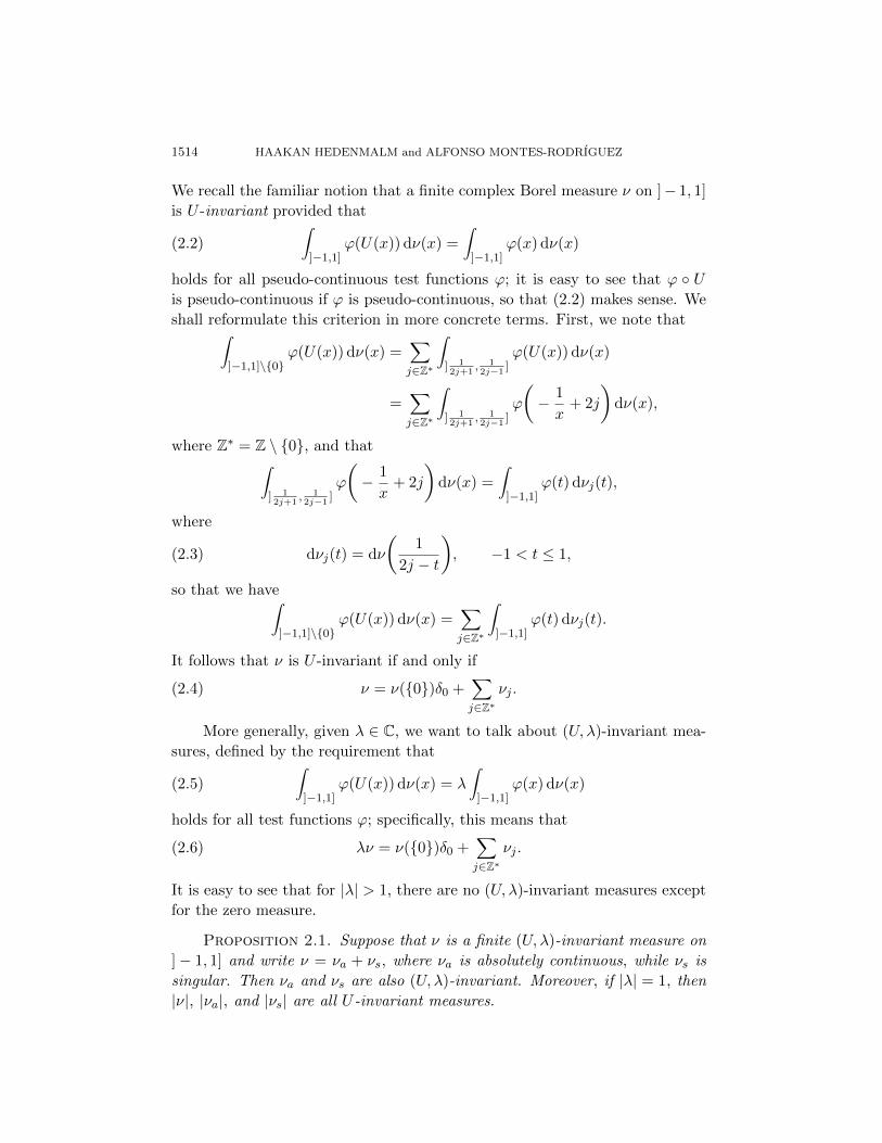
We recall the familiar notion that a finite complex Borel measure ν on ]− 1, 1]
is U -invariant provided that
(2.2)
∫]−1,1]
ϕ(U(x)) dν(x) =
∫]−1,1]
ϕ(x) dν(x)
holds for all pseudo-continuous test functions ϕ; it is easy to see that ϕ ◦ Uis pseudo-continuous if ϕ is pseudo-continuous, so that (2.2) makes sense. We
shall reformulate this criterion in more concrete terms. First, we note that∫]−1,1]\{0}
ϕ(U(x)) dν(x) =∑j∈Z∗
∫] 12j+1
, 12j−1
]ϕ(U(x)) dν(x)
=∑j∈Z∗
∫] 12j+1
, 12j−1
]ϕ
Ç− 1
x+ 2j
ådν(x),
where Z∗ = Z \ {0}, and that∫] 12j+1
, 12j−1
]ϕ
Ç− 1
x+ 2j
ådν(x) =
∫]−1,1]
ϕ(t) dνj(t),
where
(2.3) dνj(t) = dν
Ç1
2j − t
å, −1 < t ≤ 1,
so that we have∫]−1,1]\{0}
ϕ(U(x)) dν(x) =∑j∈Z∗
∫]−1,1]
ϕ(t) dνj(t).
It follows that ν is U -invariant if and only if
(2.4) ν = ν({0})δ0 +∑j∈Z∗
νj .
More generally, given λ ∈ C, we want to talk about (U, λ)-invariant mea-
sures, defined by the requirement that
(2.5)
∫]−1,1]
ϕ(U(x)) dν(x) = λ
∫]−1,1]
ϕ(x) dν(x)
holds for all test functions ϕ; specifically, this means that
(2.6) λν = ν({0})δ0 +∑j∈Z∗
νj .
It is easy to see that for |λ| > 1, there are no (U, λ)-invariant measures except
for the zero measure.
Proposition 2.1. Suppose that ν is a finite (U, λ)-invariant measure on
]− 1, 1] and write ν = νa + νs, where νa is absolutely continuous, while νs is
singular. Then νa and νs are also (U, λ)-invariant. Moreover, if |λ| = 1, then
|ν|, |νa|, and |νs| are all U -invariant measures.
HEISENBERG UNIQUENESS PAIRS AND THE KLEIN-GORDON EQUATION 1515
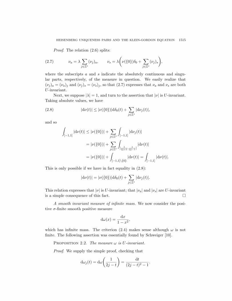
Proof. The relation (2.6) splits:
(2.7) νa = λ∑j∈Z∗
(νj)a, νs = λ
Çν({0})δ0 +
∑j∈Z∗
(νj)s
å,
where the subscripts a and s indicate the absolutely continuous and singu-
lar parts, respectively, of the measure in question. We easily realize that
(νj)a = (νa)j and (νj)s = (νs)j , so that (2.7) expresses that νa and νs are both
U -invariant.
Next, we suppose |λ| = 1, and turn to the assertion that |ν| is U -invariant.
Taking absolute values, we have
(2.8) |dν(t)| ≤ |ν({0})|dδ0(t) +∑j∈Z∗|dνj(t)|,
and so ∫]−1,1]
|dν(t)| ≤ |ν({0})|+∑j∈Z∗
∫]−1,1]
|dνj(t)|
= |ν({0})|+∑j∈Z∗
∫] 12j+1
, 12j−1
]|dν(t)|
= |ν({0})|+∫
]−1,1]\{0}|dν(t)| =
∫]−1,1]
|dν(t)|.
This is only possible if we have in fact equality in (2.8):
|dν(t)| = |ν({0})|dδ0(t) +∑j∈Z∗|dνj(t)|.
This relation expresses that |ν| is U -invariant; that |νa| and |νs| are U -invariant
is a simple consequence of this fact. �
A smooth invariant measure of infinite mass. We now consider the posi-
tive σ-finite smooth positive measure
dω(x) =dx
1− x2,
which has infinite mass. The criterion (2.4) makes sense although ω is not
finite. The following assertion was essentially found by Schweiger [10].
Proposition 2.2. The measure ω is U -invariant.
Proof. We supply the simple proof, checking that
dωj(t) = dω
Ç1
2j − t
å=
dt
(2j − t)2 − 1.
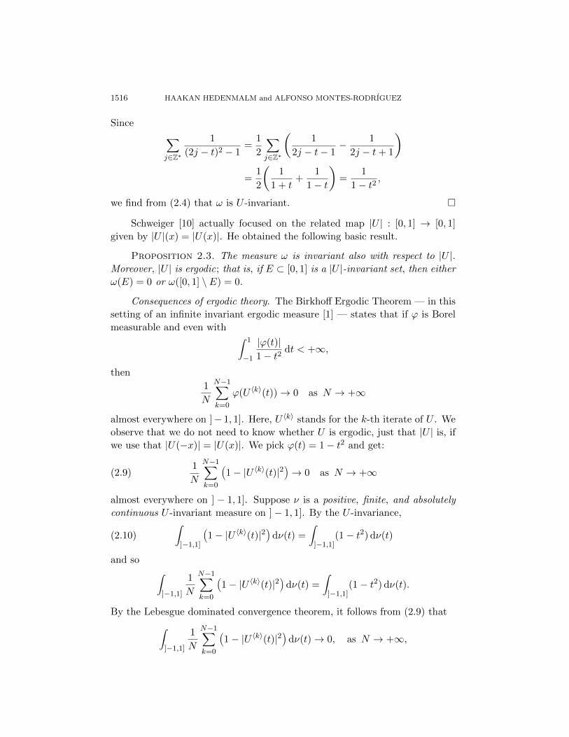
1516 HAAKAN HEDENMALM and ALFONSO MONTES-RODRIGUEZ
Since ∑j∈Z∗
1
(2j − t)2 − 1=
1
2
∑j∈Z∗
Ç1
2j − t− 1− 1
2j − t+ 1
å=
1
2
Ç1
1 + t+
1
1− t
å=
1
1− t2,
we find from (2.4) that ω is U -invariant. �
Schweiger [10] actually focused on the related map |U | : [0, 1] → [0, 1]
given by |U |(x) = |U(x)|. He obtained the following basic result.
Proposition 2.3. The measure ω is invariant also with respect to |U |.Moreover, |U | is ergodic; that is, if E ⊂ [0, 1] is a |U |-invariant set, then either
ω(E) = 0 or ω([0, 1] \ E) = 0.
Consequences of ergodic theory. The Birkhoff Ergodic Theorem — in this
setting of an infinite invariant ergodic measure [1] — states that if ϕ is Borel
measurable and even with ∫ 1
−1
|ϕ(t)|1− t2
dt < +∞,
then
1
N
N−1∑k=0
ϕ(U 〈k〉(t))→ 0 as N → +∞
almost everywhere on ]− 1, 1]. Here, U 〈k〉 stands for the k-th iterate of U . We
observe that we do not need to know whether U is ergodic, just that |U | is, if
we use that |U(−x)| = |U(x)|. We pick ϕ(t) = 1− t2 and get:
(2.9)1
N
N−1∑k=0
Ä1− |U 〈k〉(t)|2
ä→ 0 as N → +∞
almost everywhere on ] − 1, 1]. Suppose ν is a positive, finite, and absolutely
continuous U -invariant measure on ]− 1, 1]. By the U -invariance,
(2.10)
∫]−1,1]
Ä1− |U 〈k〉(t)|2
ädν(t) =
∫]−1,1]
(1− t2) dν(t)
and so ∫]−1,1]
1
N
N−1∑k=0
Ä1− |U 〈k〉(t)|2
ädν(t) =
∫]−1,1]
(1− t2) dν(t).
By the Lebesgue dominated convergence theorem, it follows from (2.9) that∫]−1,1]
1
N
N−1∑k=0
Ä1− |U 〈k〉(t)|2
ädν(t)→ 0, as N → +∞,
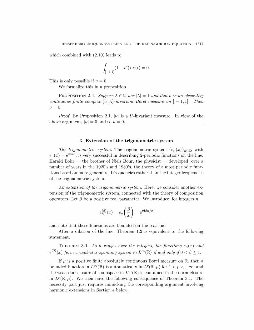
HEISENBERG UNIQUENESS PAIRS AND THE KLEIN-GORDON EQUATION 1517
which combined with (2.10) leads to∫]−1,1]
(1− t2) dν(t) = 0.
This is only possible if ν = 0.
We formalize this in a proposition.
Proposition 2.4. Suppose λ ∈ C has |λ| = 1 and that ν is an absolutely
continuous finite complex (U, λ)-invariant Borel measure on ] − 1, 1]. Then
ν = 0.
Proof. By Proposition 2.1, |ν| is a U -invariant measure. In view of the
above argument, |ν| = 0 and so ν = 0. �
3. Extension of the trigonometric system
The trigonometric system. The trigonometric system {en(x)}n∈Z, with
en(x) = eπinx, is very successful in describing 2-periodic functions on the line.
Harald Bohr — the brother of Niels Bohr, the physicist — developed, over a
number of years in the 1920’s and 1930’s, the theory of almost periodic func-
tions based on more general real frequencies rather than the integer frequencies
of the trigonometric system.
An extension of the trigonometric system. Here, we consider another ex-
tension of the trigonometric system, connected with the theory of composition
operators. Let β be a positive real parameter. We introduce, for integers n,
e〈β〉n (x) = en
Çβ
x
å= eπiβn/x
and note that these functions are bounded on the real line.
After a dilation of the line, Theorem 1.2 is equivalent to the following
statement.
Theorem 3.1. As n ranges over the integers, the functions en(x) and
e〈β〉n (x) form a weak-star-spanning system in L∞(R) if and only if 0 < β ≤ 1.
If µ is a positive finite absolutely continuous Borel measure on R, then a
bounded function in L∞(R) is automatically in Lp(R, µ) for 1 < p < +∞, and
the weak-star closure of a subspace in L∞(R) is contained in the norm closure
in Lp(R, µ). We then have the following consequence of Theorem 3.1. The
necessity part just requires mimicking the corresponding argument involving
harmonic extensions in Section 4 below.
1518 HAAKAN HEDENMALM and ALFONSO MONTES-RODRIGUEZ
Corollary 3.2. Suppose 1 < p < +∞ and that dµ(x) = M(x)dx, where
M(x) ≥ 0 is Borel measurable, with
0 <
∫ +∞
−∞M(x) dx < +∞.
Then, as n ranges over the integers, the functions en(x) and e〈β〉n (x) form a
spanning system in Lp(R, µ) provided that 0 < β ≤ 1. If, in addition,∫ +∞
−∞
dx
(1 + x2)p/(p−1)M(x)1/(p−1)< +∞,
the condition 0 < β ≤ 1 is also necessary in order to have a spanning system.
4. Necessity of the condition 0 < β ≤ 1
Harmonic extension. We extend the functions en harmonically and bound-
edly to the upper half-plane C+ = {z ∈ C : Im z > 0}:
en(z) = eπinz, Im z ≥ 0, n ≥ 0,
while
en(z) = eπinz, Im z ≥ 0, n < 0.
Likewise, the harmonic extension of e〈β〉n is
e〈β〉n (z) = eπiβn/z, Im z ≥ 0, n ≥ 0,
and
e〈β〉n (z) = eπiβn/z, Im z ≥ 0, n < 0.
Point separation. A general L∞(R) function is extended harmonically and
boundedly to C+ via the Poisson kernel; for each z0 = x0 +iy0 ∈ C+, the point
evaluation functional f 7→ f(z0) is given by
f(z0) =1
π
∫ +∞
−∞P (t, z0) f(t) dt, P (t, z0) =
y0
(x0 − t)2 + y20
,
where t 7→ P (t, z0) is in L1(R). The functional is therefore weak-star contin-
uous on L∞(R). As we harmonically extend all the functions in L∞(R), we
get the space of all bounded harmonic functions in C+. The bounded har-
monic functions in C+ separate the points of C+, so if we can find two points
z1, z2 ∈ C+ with z1 6= z2, such that
(4.1) en(z1) = en(z2), e〈β〉n (z1) = e〈β〉n (z2),
for all n ∈ Z, then the linear span of en, e〈β〉n cannot be weak-star dense in
L∞(R). The condition (4.1) boils down to
z1 − z2 ∈ 2Z,1
z1− 1
z2∈ 2
βZ,
HEISENBERG UNIQUENESS PAIRS AND THE KLEIN-GORDON EQUATION 1519
where we may apply Lemma 1.5, with m = n = 1, a = 2, and b = 2/β.
Assuming that 1 < β < +∞, we get that
z1 = 1 + i√β − 1, z2 = −1 + i
√β − 1,
are points in C+ satisfying (4.1). It follows that the requirement 0 < β ≤ 1 is
necessary in Theorem 3.1.
5. Periodic and inverted-periodic functions
Periodic and inverted-periodic functions. The weak-star closure in L∞(R)
of the linear span of the functions en(x) = eπinx, n ∈ Z, equals L∞2 (R), the
subspace of 2-periodic functions. Similarly, the weak-star closure of the linear
span of the functions e〈β〉(x) = en(β/x), n ∈ Z, equals the subspace L∞〈β〉(R)
of all functions f ∈ L∞(R) with x 7→ f(β/x) being 2-periodic. Let us tacitly
extend all functions in L∞(R) harmonically to C+ using the Poisson kernel.
The intersection space. Let us, for a moment, consider the intersection
L∞2 (R) ∩ L∞〈β〉(R).
We introduce G(β) as the group of Mobius transformations preserving C+ gen-
erated by the translation z 7→ z + 2 and the mapping z 7→ βz/(β − 2z); then
the elements of L∞2 (R) ∩ L∞〈β〉(R) are precisely the functions in L∞(R) that
are invariant under f 7→ f ◦ γ, for γ ∈ G(β). This situation is investigated
in Section 11.4 of Beardon’s book [2]. For 0 < β ≤ 1, the group G(β) is dis-
crete and free (see, e.g., Gilman and Maskit [4]), and the fundamental domain
(hyperbolic polygon) associated with C+/G(β) is given by
(5.1) D(β) =
®z ∈ C+ : |Re z| < 1,
∣∣∣∣∣z − β
2
∣∣∣∣∣ > β
2,
∣∣∣∣∣z +β
2
∣∣∣∣∣ > β
2
´.
The domain D(β) has a cusp at infinity and at the origin. In addition, it has
cusp(s) at ±1 for β = 1. For 0 < β < 1, the fundamental domain has two
boundary line segments ]− 1,−β[ and ]β, 1[, which is enough for C+/G(β) to
carry plenty of bounded harmonic (holomorphic as well) functions. A cusp is
a removable singularity for a bounded harmonic function on C+/G(β) (it is
just an isolated removed point on the Riemann surface), which means that only
constants are bounded and harmonic on C+/G(β) for β = 1. For 1 < β < +∞,
the group G(β) is discrete if and only if
(5.2) β =1
cos2(pπ/(2q))
for some coprime positive integers p, q with p < q and p ∈ {1, 2}. In case p = 1,
the fundamental domain is still given by (5.1), while for p = 2 it is smaller,
but retains two of the cusps. Anyway, under (5.2), only cusps (two or three)
occur in C+/G(β) and all bounded harmonic functions are constant. In the
1520 HAAKAN HEDENMALM and ALFONSO MONTES-RODRIGUEZ
remaining case, when (5.2) fails, the group G(β) is nondiscrete, and then every
harmonic function which is invariant under G(β) is necessarily constant.
We gather some of the above observations in a proposition.
Proposition 5.1. L∞2 (R)∩L∞〈β〉(R) = {constants} if and only if 1 ≤ β <+∞. Moreover, for 0 < β < 1, L∞2 (R) ∩ L∞〈β〉(R) is infinite-dimensional.
The sum space. Next, we turn to the study of the sum space. In order to
obtain Theorem 3.1, we show that
L∞2 (R) + L∞〈β〉(R)
is weak-star dense in L∞(R) if and only if 0 < β ≤ 1. In Section 4, we saw
that the sum fails to be weak-star dense for 1 < β < +∞. In the sequel, we
therefore assume that 0 < β ≤ 1. We now make a basic observation. Functions
in L∞2 (R) may be prescribed freely on ] − 1, 1], but then they are uniquely
determined everywhere else, due to periodicity. Likewise, functions in L∞〈β〉(R)
are free on R\]−β, β] and extend by “periodicity” everywhere else. This allows
us to define operators S, Tβ as follows. The first operator
S : L∞(]− 1, 1])→ L∞(R\]− 1, 1])
is obtained by extending the function to be 2-periodic on R and then restricting
the extended function to R\]− 1, 1]. The second operator
Tβ : L∞(R\]− β, β])→ L∞(]− β, β])
is the analogous extension associated with the “periodicity” in L∞〈β〉(R); in
symbols, we may express it as
Tβ[f ] = (S[f ◦ Iβ]) ◦ Iβ,
where Iβ(x) = −β/x.
Next, we agree on a useful convention. For a Lebesgue measurable subset
X of the real line of positive linear measure, we identify L∞(X) with a weak-
star closed subspace of L∞(R) by extending the functions to vanish on the
complement R \X.
Lemma 5.2. If I is the identity operator and if the operator
I−TβS : L∞(]− 1, 1])→ L∞(]− 1, 1])
has weak-star dense range, then the sum space L∞2 (R) + L∞〈β〉(R) is weak-star
dense in L∞(R).
Proof. We writeR for the range of the operator I−TβS. Pick an arbitrary
F2 ∈ L∞(R\] − 1, 1]), and ask of F1 ∈ L∞(] − 1, 1]) that F1 = Tβ[F2] + R,
where R ∈ R. The set of all sums F = F1 + F2 ∈ L∞(R) obtained in this
HEISENBERG UNIQUENESS PAIRS AND THE KLEIN-GORDON EQUATION 1521
fashion is denoted by F . The following straightforward argument shows that
F is weak-star dense in L∞(R), provided that R is. Suppose K ∈ L1(R) has
〈F,K〉R = 0
for all F ∈ F . We decompose K = K1 +K2 ∈ L1(R), where
K1 ∈ L1(]− 1, 1]) and K2 ∈ L1(R\]− 1, 1]).
Then
0 = 〈F,K〉R = 〈F1,K1〉R + 〈F2,K2〉R = 〈Tβ[F2],K1〉R + 〈R,K1〉R + 〈F2,K2〉R.
We rewrite this in the form
〈R,K1〉R = −〈F2,K2〉R − 〈Tβ[F2],K1〉R.
Only the left-hand side depends on R ∈ R; by linearity, the only way this is
possible is if 〈R,K1〉R = 0 for all R ∈ R. But as R is dense, we get that
K1 = 0. The remaining relationship now reads
〈F2,K2〉R = 0.
As F2 was arbitrary, we conclude that K2 = 0 as well.
To finish the proof, we show that
F ⊂ L∞2 (R) + L∞〈β〉(R).
For F = F1 +F2 ∈ F as above, the fact that F1−Tβ[F2] = R ∈ R means that
there exists a g ∈ L∞(]− 1, 1]) such that
(5.3) g −TβS[g] = (I−TβS)[g] = F1 −Tβ[F2].
Also, let h ∈ L∞(R\]− 1, 1]) be given by
(5.4) h = F2 − S[g].
Then, by (5.4),
(5.5) F2 = h+ S[g],
so that
Tβ[F2] = Tβ[h] + TβS[g].
If we combine this with (5.3), we get
(5.6) F1 = Tβ[F2] + g −TβS[g] = Tβ[h] + TβS[g] + g −TβS[g] = g + Tβ[h].
It follows from (5.5) and (5.6) that
F = F1 + F2 = (g + Tβ[h]) + (h+ S[g])
= (g + S[g]) + (h+ Tβ[h]) ∈ L∞2 (R) + L∞〈β〉(R).
The proof is complete. �
1522 HAAKAN HEDENMALM and ALFONSO MONTES-RODRIGUEZ
The operator TβS. For x ∈ R, let {x}2 denote the number with −1 <
{x}2 ≤ 1 and x− {x} ∈ 2Z. Then, since for ϕ ∈ L∞(]− 1, 1]),
S[ϕ](x) = ϕ({x}2) 1R\]−1,1](x), x ∈ R,
where 1E denotes the characteristic function of the set E ⊂ R, we find that for
ψ ∈ L∞(R\]− β, β]),
Tβ[ψ](x) = ψ
Çβ
{β/x}2
å1]−β,β](x), x ∈ R.
It follows that
(5.7) TβS[ϕ](x) = ϕ
Ç®β
{β/x}2
´2
å1Eβ (x), x ∈ R,
where
Eβ =
®x ∈]− β, β] \ {0} :
β
{β/x}2∈ R\]− 1, 1]
´.
6. Analysis of a related composition operator
The Gauss-type map. Let Uβ be the mapping
Uβ(x) = {−β/x}2, x 6= 0,
with Uβ(0) = 0. We consider the associated compressed composition operator
Cβ : L∞(]− 1, 1])→ L∞(]− 1, 1])
given by
Cβ[f ](x) = f(Uβ(x)) 1]−β,β](x).
We quickly realize from (5.7) that
TβS = C2β
and turn to analyzing Cβ. The identity
I−TβS = I−C2β = (I+Cβ)(I−Cβ)
shows that if I+Cβ and I−Cβ both have weak-star dense range, then I−C2β
has weak-star dense range as well. By elementary Functional Analysis, the
operators I+Cβ and I−Cβ both have weak-star dense range if and only if
for λ = ±1, the (predual) adjoint
λ I−C∗β : L1(]− 1, 1])→ L1(]− 1, 1])
has null kernel, that is, if the points ±1 both fail to be eigenvalues of C∗β. The
following result shows that this is the case for 0 < β ≤ 1, making I−TβS have
weak-star dense range, and thus, in view of Lemma 5.2,
L∞2 (R) + L∞〈β〉(R)
HEISENBERG UNIQUENESS PAIRS AND THE KLEIN-GORDON EQUATION 1523
is weak-star dense in L∞(R). Given that we have verified the necessity of the
condition 0 < β ≤ 1 in the context of Theorem 3.1, the rest of the assertion of
Theorem 3.1 follows.
Proposition 6.1. For 0 < β ≤ 1, the point spectrum σp(C∗β) of C∗β :
L1(]− 1, 1])→ L1(]− 1, 1]) is contained in the open unit disk D. In particular,
±1 are not eigenvalues of C∗β .
Proof. It is clear that
σp(C∗β) ⊂ σ(C∗β) ⊂ D,
where D is the closed unit disk, so we just need to show that a λ ∈ C with
|λ| = 1 cannot be an eigenvalue.
The treatment of the cases β = 1 and 0 < β < 1 will be different.
The case β = 1. For β = 1, Uβ = U1 = U (the map we studied in §2) and
C1 is
C1[f ](x) = f(U(x)) 1]−1,1](x).
The defining relation for the (predual) adjoint C∗1 : L1(]− 1, 1])→ L1(]− 1, 1])
is∫]−1,1]
f(x)C∗1[g](x) dx = 〈C∗1[g], f〉R = 〈g,C1[f ]〉R =
∫]−1,1]
f(U(x)) g(x) dx.
If g is a nontrivial eigenfunction for C∗1 with eigenvalue λ, then C∗1[g] = λg
and so
λ
∫]−1,1]
f(x) g(x) dx =
∫]−1,1]
f(U(x)) g(x) dx;
this expresses that the absolutely continuous finite measure dν(x) = g(x)dx
is a (U, λ)-invariant measure. By Proposition 2.4, there are no finite (U, λ)-
invariant measures except the null measure, for |λ| = 1. Consequently, λ ∈ Cis not an eigenvalue of C∗1 for |λ| = 1.
The case 0 < β < 1. The same analysis reduces the problem to studying
the absolutely continuous finite measures ν on ]− 1, 1] with
(6.1) λ
∫]−1,1]
f(t) dν(t) =
∫]−1,1]
Cβ[f ](t) dν(t) =
∫]−β,β]
f(Uβ(t)) dν(t)
for all f ∈ L∞(] − 1, 1]), where λ ∈ C is fixed with |λ| = 1. In more concrete
terms, this amounts to
λ dν(t) =∑j∈Z∗
dνj(t), t ∈]− 1, 1],
where
dνj(t) = dν
Çβ
2j − t
å, t ∈]− 1, 1].
1524 HAAKAN HEDENMALM and ALFONSO MONTES-RODRIGUEZ
Taking absolute values, we have, for |λ| = 1,
|dν(t)| ≤∑j∈Z∗|dνj(t)|, t ∈]− 1, 1].
Integrating over ]− 1, 1], we find that∫]−1,1]
|dν(t)| ≤∑j∈Z∗
∫]−1,1]
|dνj(t)| =∫
[−β,β]|dν(t)|, t ∈]− 1, 1],
which is only possible if we have the equality
|dν(t)| =∑j∈Z∗|dνj(t)|, t ∈]− 1, 1],
as well as
dν(t) = 0, t ∈]− 1, 1] \ [−β, β].
If we iterate the relation (6.1), we get
(6.2) λn∫
]−1,1]f(t) dν(t) =
∫]−1,1]
Cnβ[f ](t) dν(t) =
∫Eβ(n)
f(U〈n〉β (t)) dν(t),
where set Eβ(n) is given by
Eβ(n) =¶t ∈]− 1, 1] : U
〈k〉β (t) ∈ [−β, β] for k = 0, . . . , n− 1
©.
A repetition of the above argument involving U〈n〉β in place of Uβ shows that
if |λ| = 1, then
dν(t) = 0, t ∈]− 1, 1] \ Eβ(n).
As n→ +∞, the set Eβ(n) shrinks down to
Eβ(∞) =¶t ∈]− 1, 1] : U
〈k〉β (t) ∈ [−β, β] for k = 0, 1, 2, 3, . . .
©.
This final set Eβ(∞) is Uβ-invariant, and it is not hard to show that it must
have zero length. But the measure ν vanishes everywhere else, and being
absolutely continuous, it must be the zero measure. In particular, λ ∈ C with
|λ| = 1 cannot be eigenvalues of C∗β. The proof is complete. �
A remark on model subspaces. Given an inner function Θ in the upper half-
plane C+, one considers the model subspaces KΘ(C+) = H2(C+)ΘH2(C+).
Uniqueness sets for model subspaces have been studied recently by Makarov
and Poltoratski [8], and the injectivity of the Toeplitz operator with symbol
ΘBΛ is equivalent to Λ ⊂ C+ being a uniqueness set. In our setting, we use
mainly that the operators λ I−C∗β are injective for λ = ±1, so that appar-
ently, these operators are analogous to the Toeplitz operators from the model
subspace case.
HEISENBERG UNIQUENESS PAIRS AND THE KLEIN-GORDON EQUATION 1525
7. Applications and open problems
An application to BMO. Let BMOA(C+) be the (weak-star closed) sub-
space of the space BMO(R) consisting of functions whose Poisson extensions
to C+ are holomorphic in C+. We recall that BMO(R) denotes the space of
functions with bounded mean oscillation. The Cauchy-Szego (analytic) pro-
jection
P : L∞(R)→ BMOA(C+)
is bounded and surjective. Here, we think of BMOA(C+) as the dual ofH1(C+)
with respect to the sesquilinear form of L2(R); in particular, BMOA(C+) is
a space of functions modulo the constants. We observe that if X is a linear
subspace of L∞(R) which is weak-star dense, then P(X ) is is weak-star dense
in BMOA(C+). Moreover, let BMOA2(C+) be the subspace of BMOA(C+) of
functions invariant under z 7→ z+ 2, and let BMOA〈β〉(C+) be the subspace of
BMOA(C+) of functions invariant under z 7→ βz/(β − 2z). We quickly check
that P maps L∞2 (R)→ BMOA2(C+) and L∞〈β〉(R)→ BMOA〈β〉(C+).
In view of our main theorem (Theorem 3.1), we have the following.
Corollary 7.1. The sum BMOA2(C+) + BMOA〈β〉(C+) is weak-star
dense in BMOA(C+) if and only if 0 < β ≤ 1. In other words, the functions
en(x) = eπinx, e〈β〉−n(x) = e−πβin/x, n = 0, 1, 2, 3, . . .
span a weak-star dense subspace of BMOA(C+) if and only if 0 < β ≤ 1.
By the Mobius invariance of BMO, we may transfer this result to the
setting of the unit disk and answer Problem 2 of Matheson and Stessin [9] in
the affirmative.
Four open problems. (a) Suppose that in the context of Theorem 1.2 we
consider a lattice-cross
Λ = ((αZ + {θ})× {0}) ∪ ({0} × βZ),
where θ ∈ R is fixed. It seems that Theorem 1.2 should remain true with this
new Λ, with only moderate modifications in the proof. But what happens if
the lattice-cross is less regular, that is, if the two spacings α and β are allowed
to fluctuate a bit along the cross?
(b) In the context of Corollary 3.2, as n ranges over the integers, do
the functions en(x) and e〈β〉n (x) form a spanning system in Lp(R, µ) for all
0 < β < +∞ provided that∫ +∞
−∞
dx
(1 + x2)p/(p−1)M(x)1/(p−1)= +∞?
1526 HAAKAN HEDENMALM and ALFONSO MONTES-RODRIGUEZ
(c) Let H∞2 (C+) denote the (weak-star closed) subspace of L∞2 (R) con-
sisting of those functions whose Poisson extensions to the upper half-plane C+
are analytic. Analogously, let H∞〈β〉(C+) be the (weak-star closed) subspace of
L∞〈β〉(R) consisting of those functions whose Poisson extensions to the upper
half-plane C+ are analytic. Is the sum
H∞2 (C+) +H∞〈β〉(C+)
weak-star dense in H∞(C+) for 0 < β ≤ 1? This does not seem to follow from
our Theorem 3.1, and, if answered in the affirmative (for 0 < β < 1), it would
solve Problem 1 of [9].
(d) In the context of Corollary 1.3, let the finite Borel measure µ be sup-
ported on the hyperbola x1x2 = ε and let Λ be the lattice-cross given by the
positive parameters α, β. If µ is absolutely continuous with respect to arc
length measure on the hyperbola, an argument involving curvature considera-
tions shows that
µ(ξ)→ 0 as |ξ| → +∞.
In a sense, this expresses the absence of point masses in µ. Moreover, µ solves
the Klein-Gordon equation ∂1∂2µ+επ2µ = 0. It would be desirable to remove,
to the extent possible, the Fourier analysis ingredient in Corollary 1.3. Let
u be a bounded continuous complex-valued function on R2 with u(ξ) → 0 as
|ξ| → +∞. Suppose, in addition, that ∂1∂2u+ επ2u = 0 holds in the sense of
distribution theory. The problem: is the lattice-cross Λ, with αβ ≤ 1/|ε|, a
uniqueness set for u (that is, u|Λ = 0 =⇒ u = 0)?
Acknowledgements. We thank Dani Blasi Babot, Francesco Cellarosi,
Joaquim Ortega-Cerda, Eero Saksman, Masha Saprykina, Serguei Shimorin,
and Yakov Sinai for helpful comments and references.
References
[1] J. Aaronson, An Introduction to Infinite Ergodic Theory, Math. Surveys
Monogr. 50, Amer. Math. Soc., Providence, RI, 1997. MR 1450400. Zbl 0882.
28013.
[2] A. F. Beardon, The Geometry of Discrete Groups, Grad. Texts in Math. 91,
Springer-Verlag, New York, 1983. MR 0698777. Zbl 0528.30001.
[3] F. Cellarosi, Renewal-type limit theorem for continued fractions with even
partial quotients, Ergodic Theory Dynam. Systems 29 (2009), 1451–1478.
MR 2545013. Zbl 1193.37013. doi: 10.1017/S0143385708000825.
[4] J. Gilman and B. Maskit, An algorithm for 2-generator Fuchsian groups,
Michigan Math. J. 38 (1991), 13–32. MR 1091506. Zbl 0724.20033. doi:
10.1307/mmj/1029004258.
HEISENBERG UNIQUENESS PAIRS AND THE KLEIN-GORDON EQUATION 1527
[5] V. Havin and B. Joricke, The Uncertainty Principle in Harmonic Analy-
sis, Ergeb. Math. Grenzgeb. 28, Springer-Verlag, New York, 1994. MR 1303780.
Zbl 0827.42001.
[6] W. Heisenberg, Uber den anschaulichen Inhalt der quantentheoretischen Kine-
matik und Mechanik, Z. Physik 43 (1927), 172–198. JFM 53.0853.05.
[7] C. Kraaikamp and A. Lopes, The theta group and the continued fraction
expansion with even partial quotients, Geom. Dedicata 59 (1996), 293–333.
MR 1371228. Zbl 0841.58049. doi: 10.1007/BF00181695.
[8] N. Makarov and A. Poltoratski, Meromorphic inner functions, Toeplitz ker-
nels and the uncertainty principle, in Perspectives in Analysis, Math. Phys. Stud.
27, Springer-Verlag, New York, 2005, pp. 185–252. MR 2215727. Zbl 1118.47020.
doi: 10.1007/3-540-30434-7_10.
[9] A. L. Matheson and M. I. Stessin, Cauchy transforms of characteris-
tic functions and algebras generated by inner functions, Proc. Amer. Math.
Soc. 133 (2005), 3361–3370. MR 2161161. Zbl 1087.46019. doi: 10.1090/
S0002-9939-05-07913-X.
[10] F. Schweiger, Continued fractions with odd and even partial quotients, Ar-
beitsberichte Math. Institut Universtat Salzburg 4 (1982), 59–70.
[11] , On the approximation by continued fractions with odd and even partial
quotients, Arbeitsberichte Math. Institut Universtat Salzburg 1-2 (1984), 105–114.
(Received: September 25, 2008)
(Revised: January 12, 2009)
Royal Institute of Technology, Stockholm, Sweden
E-mail : [email protected]
http://www.math.kth.se/∼haakanh
University of Sevilla, Sevilla,Spain
E-mail : [email protected]