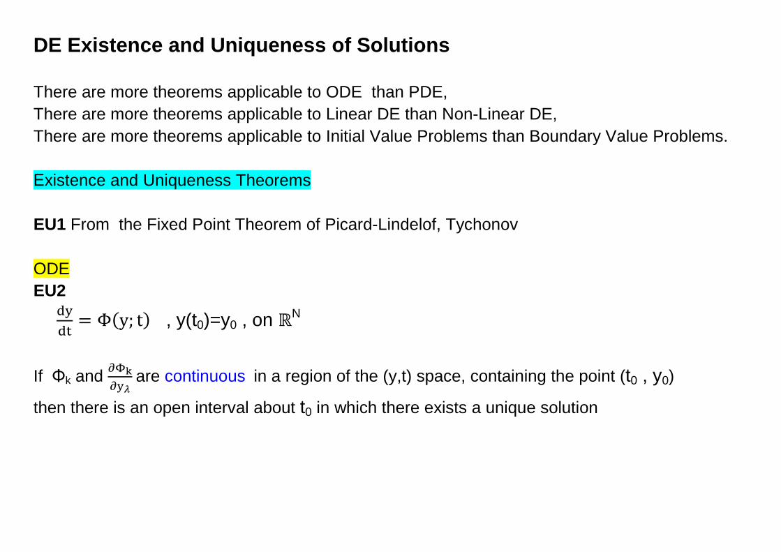
DE Existence and Uniqueness of Solutions There are more theorems applicable to ODE than PDE, There are more theorems applicable to Linear DE than Non-Linear DE, There are more theorems applicable to Initial Value Problems than Boundary Value Problems. Εxistence and Uniqueness Theorems EU1 From the Fixed Point Theorem of Picard-Lindelof, Tychonov ODE EU2

dydt

= Φ(y; t) , y(t0)=y0 , on ℝN

If Φk and ∂Φk

∂y𝜆 are continuous in a region of the (y,t) space, containing the point (t0 , y0)

then there is an open interval about t0 in which there exists a unique solution

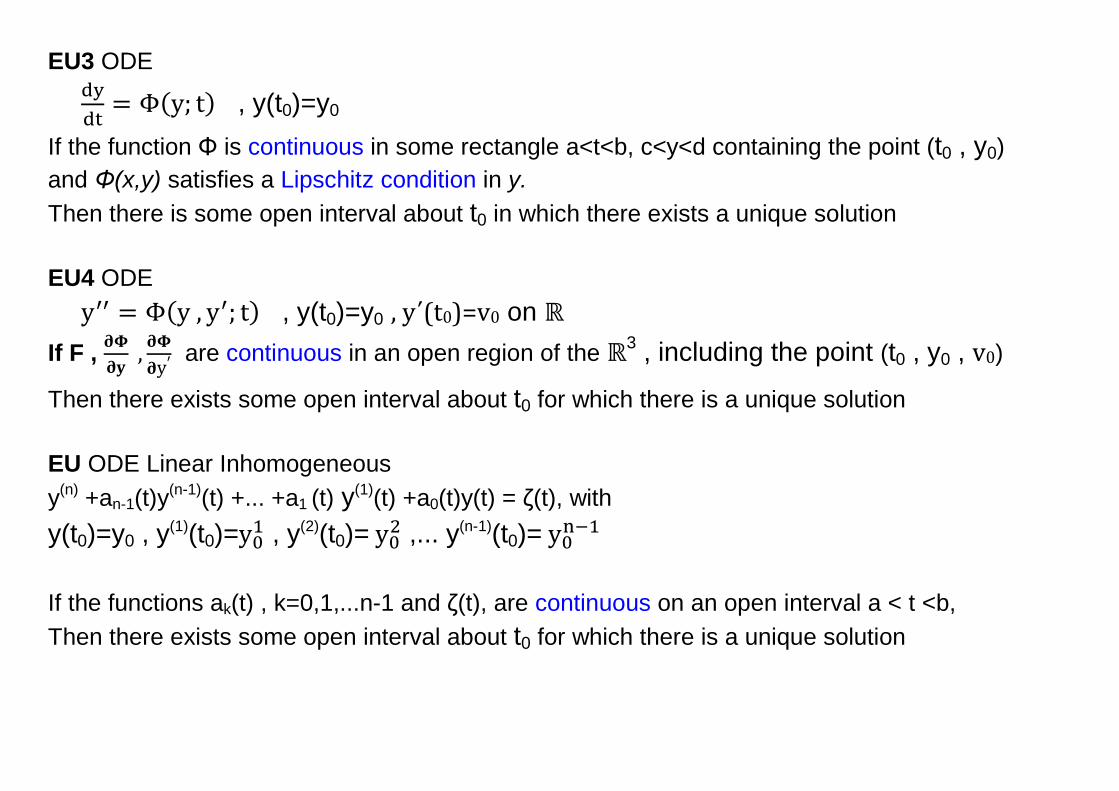
EU3 ODE

dydt

= Φ(y; t) , y(t0)=y0

If the function Φ is continuous in some rectangle a<t<b, c<y<d containing the point (t0 , y0) and Φ(x,y) satisfies a Lipschitz condition in y. Then there is some open interval about t0 in which there exists a unique solution EU4 ODE y′′ = Φ(y , y′; t) , y(t0)=y0 , y΄(t0)=v0 on ℝ

If F , 𝛛𝚽𝛛𝐲

, 𝛛𝚽𝛛y′ are continuous in an open region of the ℝ3 , including the point (t0 , y0 , v0)

Then there exists some open interval about t0 for which there is a unique solution EU ODE Linear Inhomogeneous y(n) +an-1(t)y(n-1)(t) +... +a1 (t) y(1)(t) +a0(t)y(t) = ζ(t), with y(t0)=y0 , y(1)(t0)=y0

1 , y(2)(t0)= y02 ,... y(n-1)(t0)= y0

n−1 If the functions ak(t) , k=0,1,...n-1 and ζ(t), are continuous on an open interval a < t <b, Then there exists some open interval about t0 for which there is a unique solution

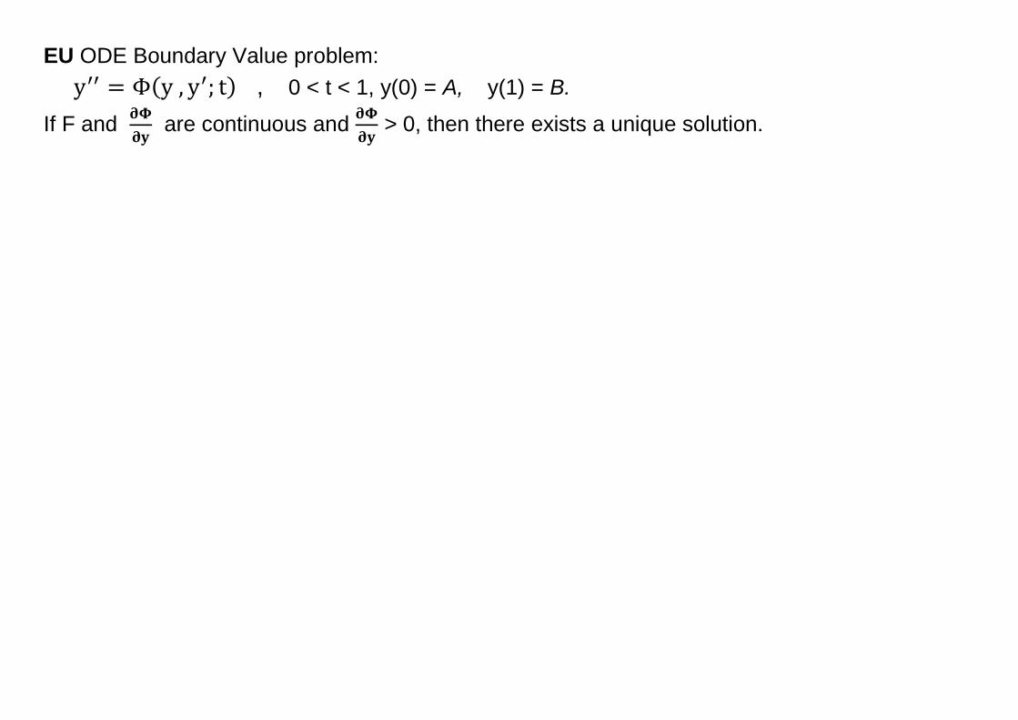
EU ODE Boundary Value problem: y′′ = Φ(y , y′; t) , 0 < t < 1, y(0) = A, y(1) = B.

If F and 𝛛𝚽𝛛𝐲

are continuous and 𝛛𝚽𝛛𝐲

> 0, then there exists a unique solution.

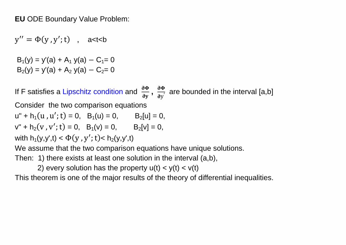
EU ODE Boundary Value Problem: y′′ = Φ(y , y′; t) , a<t<b B1(y) = y'(a) + A1 y(a) − C1= 0 B2(y) = y'(a) + A2 y(a) − C2= 0 If F satisfies a Lipschitz condition and 𝛛𝚽

𝛛𝐲 , 𝛛𝚽

𝛛y′ are bounded in the interval [a,b]

Consider the two comparison equations u" + h1(u , u′; t) = 0, B1(u) = 0, B2[u] = 0, v" + h2(v , v′; t) = 0, B1(v) = 0, B2[v] = 0, with h1(y,y',t) < Φ(y , y′; t)< h2(y,y',t) We assume that the two comparison equations have unique solutions. Then: 1) there exists at least one solution in the interval (a,b), 2) every solution has the property u(t) < y(t) < v(t) This theorem is one of the major results of the theory of differential inequalities.

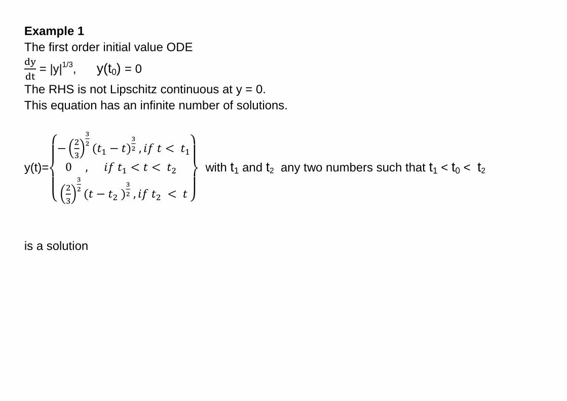
Example 1 The first order initial value ODE dydt

= |y|1/3, y(t0) = 0

The RHS is not Lipschitz continuous at y = 0. This equation has an infinite number of solutions.

y(t)=

⎩⎪⎨

⎪⎧− �2

3�

32 (𝑡1 − 𝑡)

32 , 𝑖𝑓 𝑡 < 𝑡1

0 , 𝑖𝑓 𝑡1 < 𝑡 < 𝑡2

�23�

32 (𝑡 − 𝑡2 )

32 , 𝑖𝑓 𝑡2 < 𝑡 ⎭

⎪⎬

⎪⎫

with t1 and t2 any two numbers such that t1 < t0 < t2

is a solution

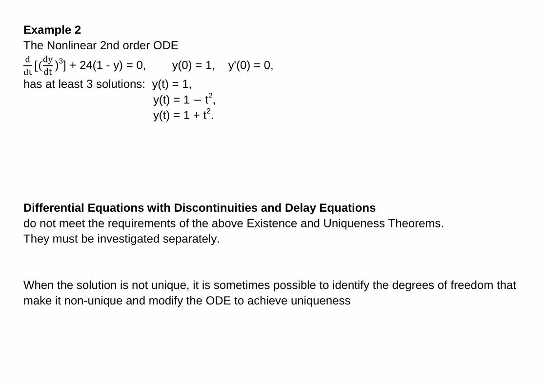
Example 2 The Nonlinear 2nd order ODE ddt

[(dydt

)3] + 24(1 - y) = 0, y(0) = 1, y'(0) = 0, has at least 3 solutions: y(t) = 1, y(t) = 1 − t2, y(t) = 1 + t2. Differential Equations with Discontinuities and Delay Equations do not meet the requirements of the above Existence and Uniqueness Theorems. They must be investigated separately. When the solution is not unique, it is sometimes possible to identify the degrees of freedom that make it non-unique and modify the ODE to achieve uniqueness

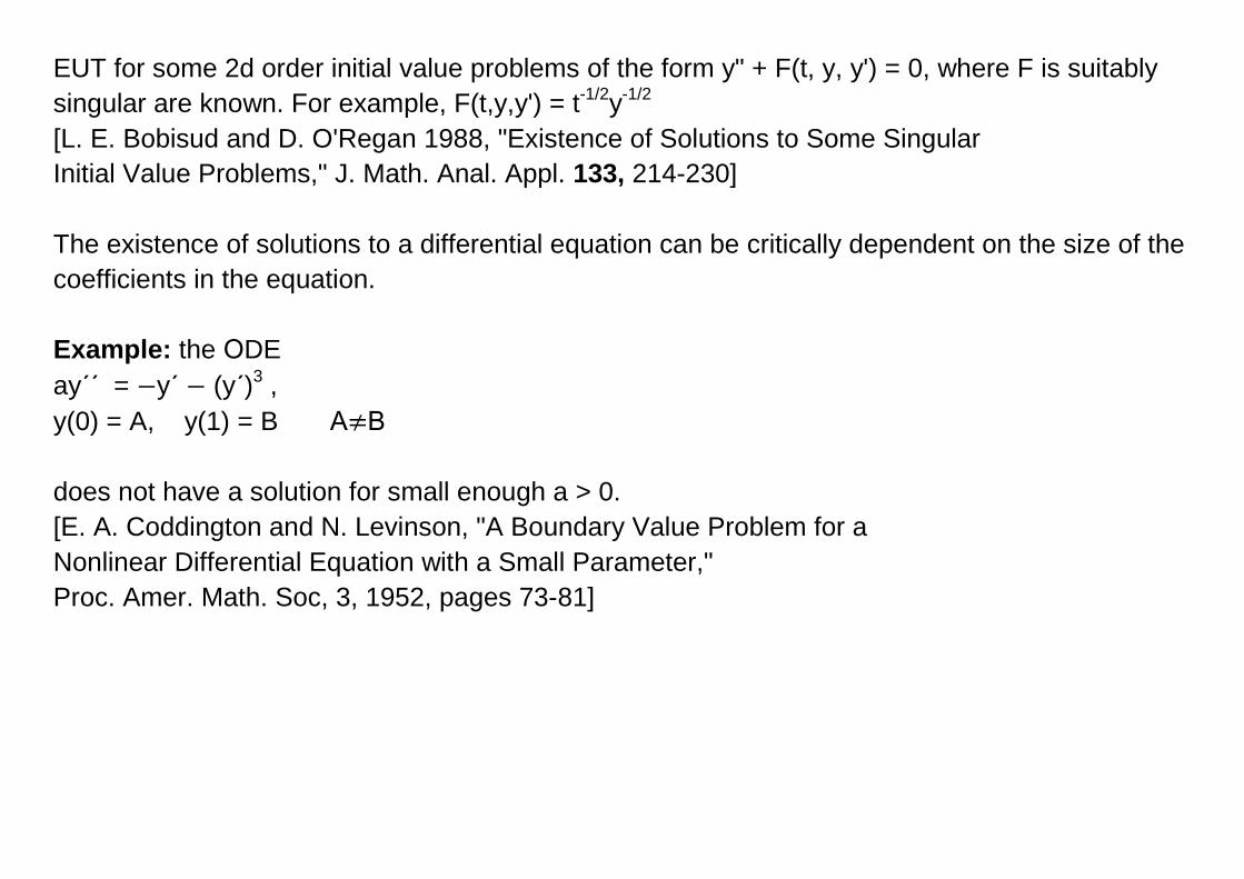
EUT for some 2d order initial value problems of the form y" + F(t, y, y') = 0, where F is suitably singular are known. For example, F(t,y,y') = t-1/2y-1/2 [L. E. Bobisud and D. O'Regan 1988, "Existence of Solutions to Some Singular Initial Value Problems," J. Math. Anal. Appl. 133, 214-230] The existence of solutions to a differential equation can be critically dependent on the size of the coefficients in the equation. Example: the ΟDE ay΄΄ = −y΄ − (y΄)3 , y(0) = A, y(1) = B Α≠Β does not have a solution for small enough a > 0. [E. A. Coddington and N. Levinson, "A Boundary Value Problem for a Nonlinear Differential Equation with a Small Parameter," Proc. Amer. Math. Soc, 3, 1952, pages 73-81]

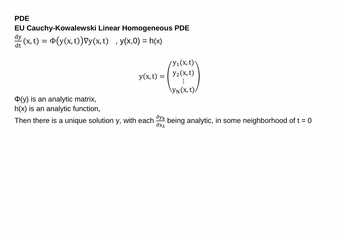
PDE EU Cauchy-Kowalewski Linear Homogeneous PDE dydt

(x, t) = Φ�y(x, t)�∇y(x, t) , y(x,0) = h(x)

y(x, t) = �

y1(x, t)y2(x, t)

⋮yN(x, t)

�

Φ(y) is an analytic matrix, h(x) is an analytic function, Then there is a unique solution y, with each ∂yk

∂x𝜆 being analytic, in some neighborhood of t = 0

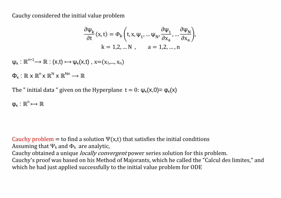
Cauchy considered the initial value problem

∂ψk∂t

(x, t) = 𝛷k �t, x,ψ1, …ψN,∂ψ1∂xa

, …∂ψN∂xa

�,

k = 1,2, … N , a = 1,2, … , n ψκ : ℝn+1⟶ ℝ : (x,t) ⟼ ψκ(x,t) , x=(x1,..., xn) Φκ : ℝ x ℝn x ℝN x ℝNn ⟶ ℝ The " initial data " given on the Hyperplane t = 0: ψκ(x,0)= φκ(x) φκ : ℝn ⟼ ℝ Cauchy problem = to find a solution Ψ(x,t) that satisfies the initial conditions Assuming that Ψk and Φk are analytic, Cauchy obtained a unique locally convergent power series solution for this problem. Cauchy's proof was based on his Method of Majorants, which he called the "Calcul des limites," and which he had just applied successfully to the initial value problem for ΟDE

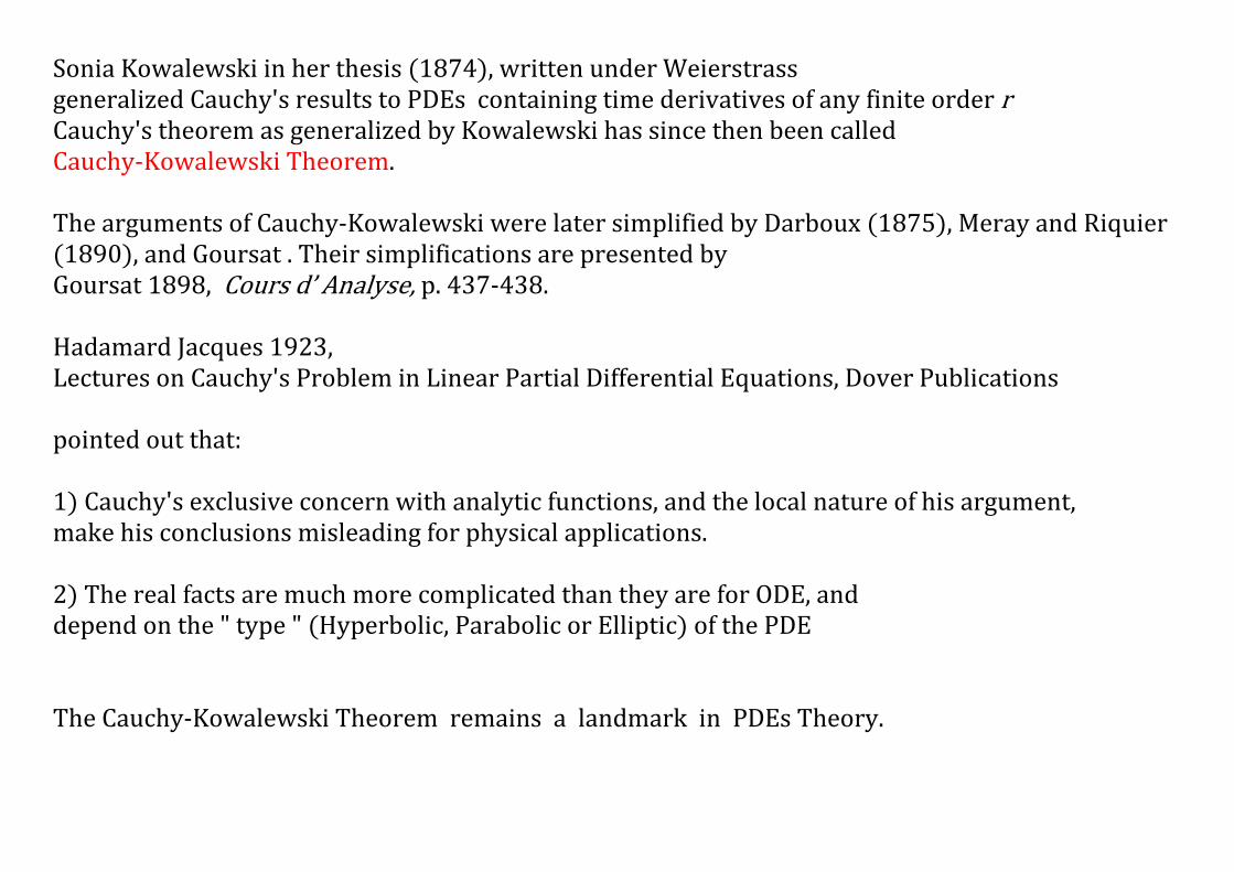
Sonia Kowalewski in her thesis (1874), written under Weierstrass generalized Cauchy's results to PDEs containing time derivatives of any finite order r Cauchy's theorem as generalized by Kowalewski has since then been called Cauchy-Kowalewski Theorem. The arguments of Cauchy-Kowalewski were later simplified by Darboux (1875), Meray and Riquier (1890), and Goursat . Their simplifications are presented by Goursat 1898, Cours d’ Analyse, p. 437-438. Hadamard Jacques 1923, Lectures on Cauchy's Problem in Linear Partial Differential Equations, Dover Publications pointed out that: 1) Cauchy's exclusive concern with analytic functions, and the local nature of his argument, make his conclusions misleading for physical applications. 2) The real facts are much more complicated than they are for ODE, and depend on the " type " (Hyperbolic, Parabolic or Elliptic) of the PDE The Cauchy-Kowalewski Theorem remains a landmark in PDEs Theory.

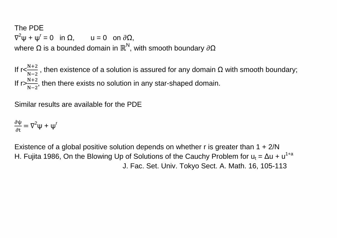
The PDΕ ∇2ψ + ψr = 0 in Ω, u = 0 on ∂Ω, where Ω is a bounded domain in ℝN, with smooth boundary ∂Ω If r<N+2

N−2 , then existence of a solution is assured for any domain Ω with smooth boundary;

If r>N+2N−2

, then there exists no solution in any star-shaped domain. Similar results are available for the PDE ∂ψ∂t

= ∇2ψ + ψr Existence of a global positive solution depends on whether r is greater than 1 + 2/N H. Fujita 1986, On the Blowing Up of Solutions of the Cauchy Problem for ut = Δu + u1+a J. Fac. Set. Univ. Tokyo Sect. A. Math. 16, 105-113

References W. E. Boyce and R. C. DiPrima 1986, Elementary Differential Equations and Boundary Value Problems, 4th Edition, John Wiley & Sons, New York, M. Feckan 1991, "A New Method for the Existence of Solution of Nonlinear Differential Equations," J. Differential Equations 89, 203-223 H. A. Levine 1990, "The Role of Critical Exponents in Blowup Theorems," SIAM Review 32, No. 2, 262-288. H. Lewy 1957, "An Example of a Smooth Linear Partial Differential Equation without Solution," Annals of Math. 66, No. 1, 155-158. M. Plum 1991, "Computer-Assisted Existence Proofs for Two-Point Boundary Value Problems," Computing 46, 19-34.

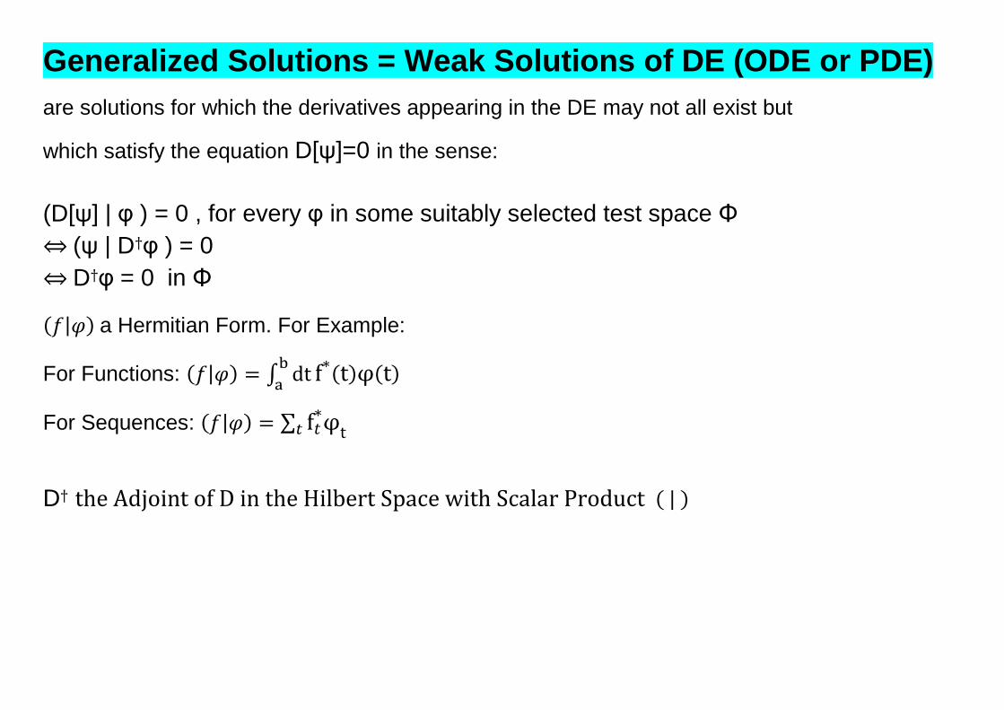
Generalized Solutions = Weak Solutions of DE (ODE or PDE) are solutions for which the derivatives appearing in the DE may not all exist but

which satisfy the equation D[ψ]=0 in the sense: (D[ψ] | φ ) = 0 , for every φ in some suitably selected test space Φ ⇔ (ψ | D†φ ) = 0 ⇔ D†φ = 0 in Φ

(𝑓|𝜑) a Hermitian Form. For Example:

For Functions: (𝑓|𝜑) = ∫ dtba f∗(t)φ(t)

For Sequences: (𝑓|𝜑) = ∑ f𝑡∗φt𝑡

D† the Adjoint of D in the Hilbert Space with Scalar Product ( | )

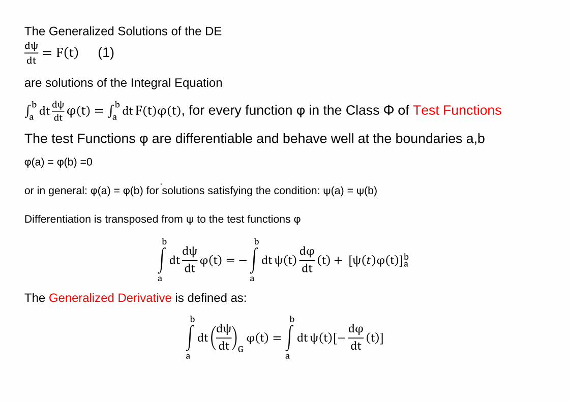
The Generalized Solutions of the DE dψdt

= F(t) (1)

are solutions of the Integral Equation

∫ dtba

dψdt φ(t) = ∫ dtb

a F(t)φ(t), for every function φ in the Class Φ οf Test Functions

The test Functions φ are differentiable and behave well at the boundaries a,b φ(a) = φ(b) =0 or in general: φ(a) = φ(b) for solutions satisfying the condition: ψ(a) = ψ(b) Differentiation is transposed from ψ to the test functions φ

� dtb

a

dψdt φ(t) = − � dt

b

a

ψ(t)dφdt

(t) + [ψ(𝑡)φ(t)]ab

The Generalized Derivative is defined as:

� dtb

a

�dψdt �

Gφ(t) = � dt

b

a

ψ(t)[−dφdt

(t)]

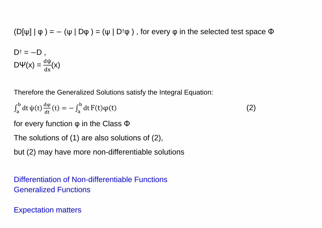
(D[ψ] | φ ) = − (ψ | Dφ ) = (ψ | D†φ ) , for every φ in the selected test space Φ D† = −D , DΨ(x) = dψ

dx(x)

Therefore the Generalized Solutions satisfy the Integral Equation:

∫ dtba ψ(t) dφ

dt(t) = − ∫ dtb

a F(t)φ(t) (2)

for every function φ in the Class Φ

The solutions of (1) are also solutions of (2),

but (2) may have more non-differentiable solutions

Differentiation of Non-differentiable Functions Generalized Functions Expectation matters

Example ODE

dψdt

= 2 , ψ(0)=0 , t in [0,1] , ψ real function on [0,1]

Solution: the differentiable function ψ(t)=2t

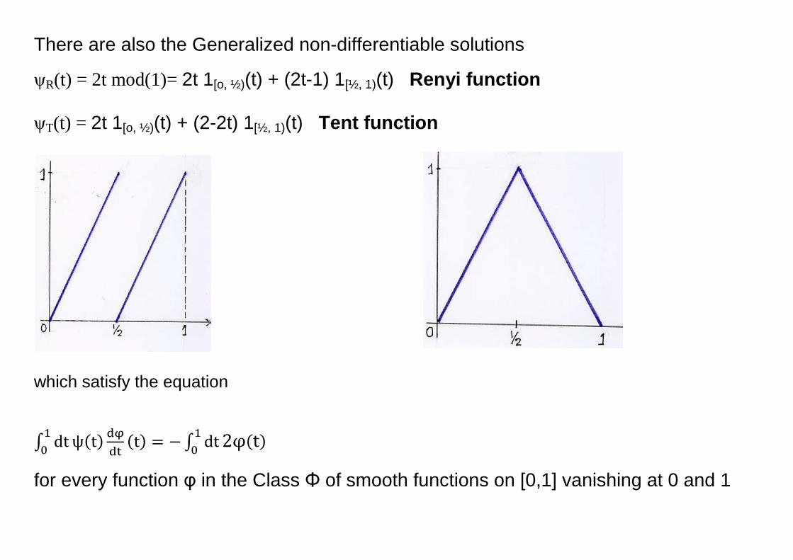
There are also the Generalized non-differentiable solutions

ψR(t) = 2t mod(1)= 2t 1[o, ½)(t) + (2t-1) 1[½, 1)(t) Renyi function ψT(t) = 2t 1[o, ½)(t) + (2-2t) 1[½, 1)(t) Tent function

which satisfy the equation

∫ dt10 ψ(t) dφ

dt(t) = − ∫ dt1

0 2φ(t)

for every function φ in the Class Φ of smooth functions on [0,1] vanishing at 0 and 1

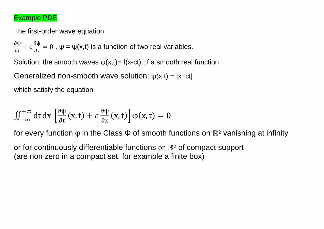
Example PDE

The first-order wave equation ∂ψ∂𝑡

+ c ∂ψ∂x

= 0 , ψ = ψ(x,t) is a function of two real variables.

Solution: the smooth waves ψ(x,t)= f(x-ct) , f a smooth real function

Generalized non-smooth wave solution: ψ(x,t) = |x−ct|

which satisfy the equation

∬ dt+∞−∞ dx �∂ψ

∂t(x, t) + 𝑐 ∂ψ

∂x(x, t)� φ(x, t) = 0

for every function φ in the Class Φ of smooth functions on ℝ2 vanishing at infinity

οr for continuously differentiable functions on ℝ2 of compact support (are non zero in a compact set, for example a finite box)

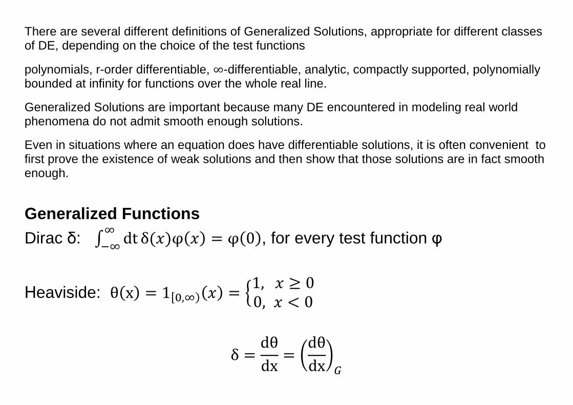
There are several different definitions of Generalized Solutions, appropriate for different classes of DE, depending on the choice of the test functions

polynomials, r-order differentiable, ∞-differentiable, analytic, compactly supported, polynomially bounded at infinity for functions over the whole real line.

Generalized Solutions are important because many DE encountered in modeling real world phenomena do not admit smooth enough solutions.

Even in situations where an equation does have differentiable solutions, it is often convenient to first prove the existence of weak solutions and then show that those solutions are in fact smooth enough.

Generalized Functions Dirac δ: ∫ dt∞

−∞ δ(𝑥)φ(𝑥) = φ(0), for every test function φ

Ηeaviside: θ(x) = 1[0,∞)(𝑥) = �1, 𝑥 ≥ 00, 𝑥 < 0

δ =dθdx

= �dθdx�

𝐺

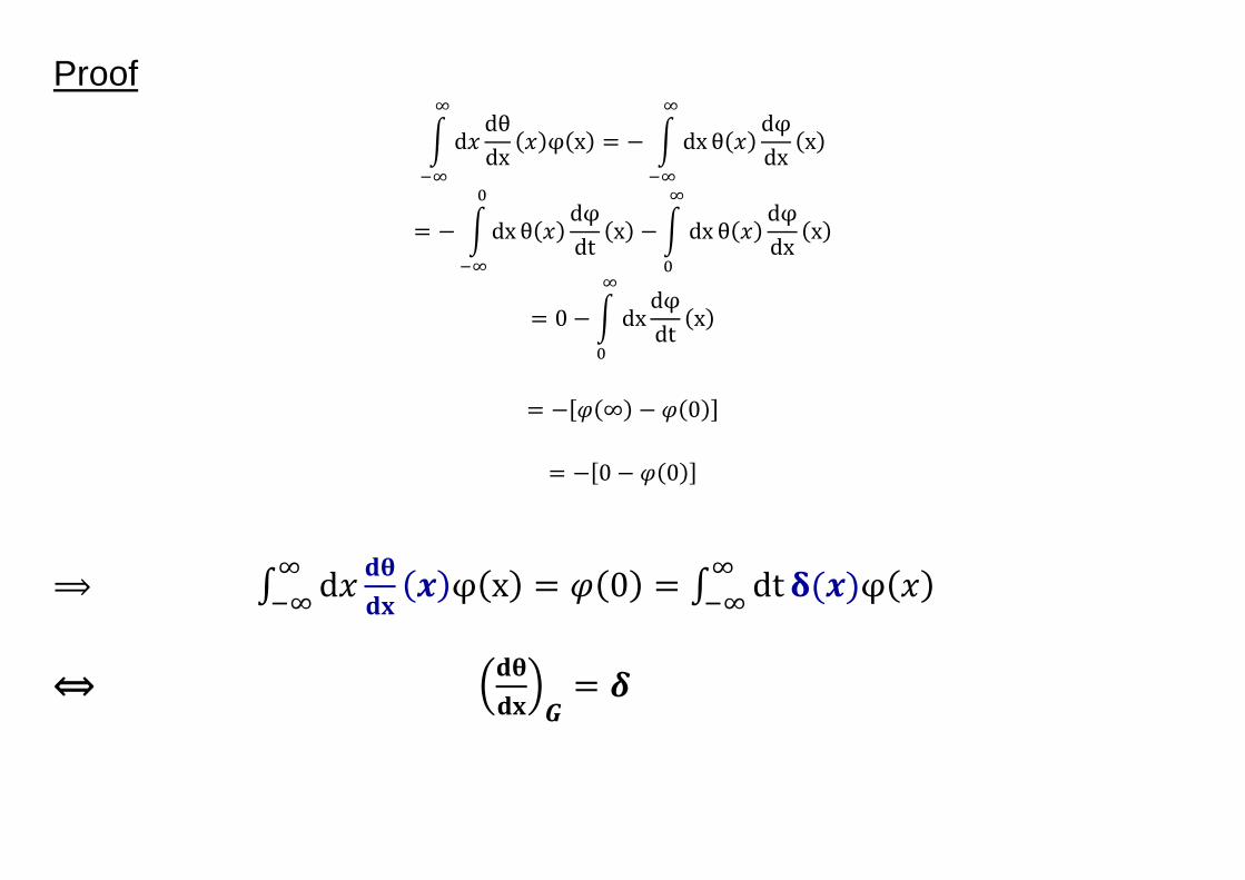
Proof

� d𝑥∞

−∞

dθdx

(𝑥)φ(x) = − � dx∞

−∞

θ(𝑥)dφdx

(x)

= − � dx0

−∞

θ(𝑥)dφdt

(x) − � dx∞

0

θ(𝑥)dφdx

(x)

= 0 − � dx∞

0

dφdt

(x)

= −[𝜑(∞) − 𝜑(0)]

= −[0 − 𝜑(0)]

⟹ ∫ d𝑥∞−∞

𝐝𝛉𝐝𝐱

(𝒙)φ(x) = 𝜑(0) = ∫ dt∞−∞ 𝛅(𝒙)φ(𝑥)

⟺ �𝐝𝛉𝐝𝐱

�𝑮

= 𝜹

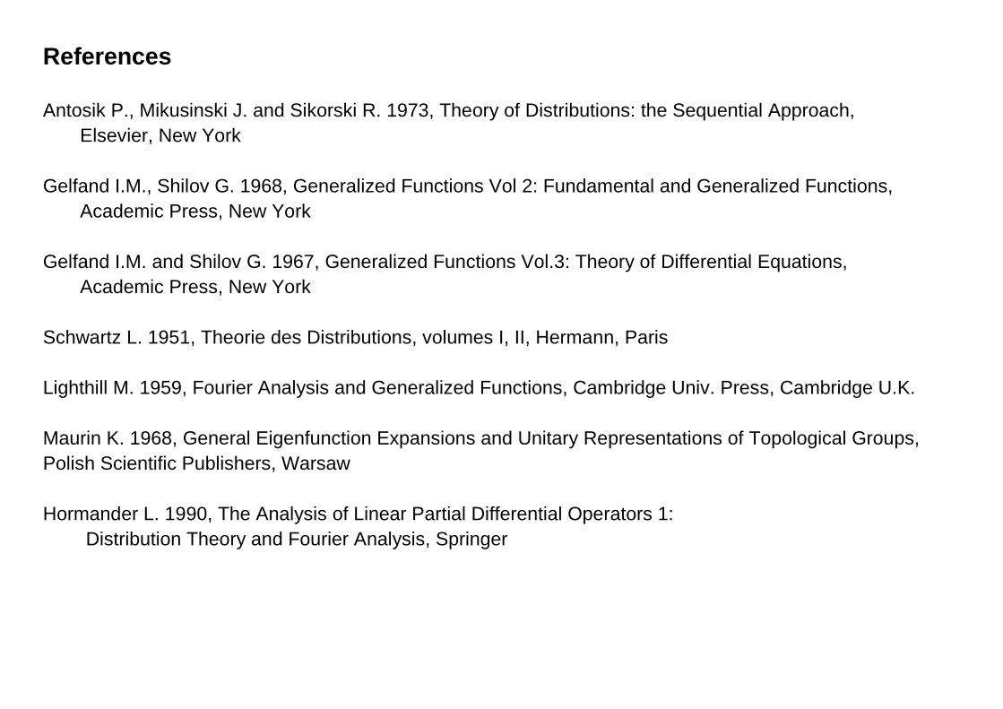
References Antosik P., Mikusinski J. and Sikorski R. 1973, Theory of Distributions: the Sequential Approach, Elsevier, New York Gelfand I.M., Shilov G. 1968, Generalized Functions Vol 2: Fundamental and Generalized Functions, Academic Press, New York Gelfand I.M. and Shilov G. 1967, Generalized Functions Vol.3: Theory of Differential Equations, Academic Press, New York Schwartz L. 1951, Theorie des Distributions, volumes I, II, Hermann, Paris Lighthill M. 1959, Fourier Analysis and Generalized Functions, Cambridge Univ. Press, Cambridge U.K. Maurin K. 1968, General Eigenfunction Expansions and Unitary Representations of Topological Groups, Polish Scientific Publishers, Warsaw Hormander L. 1990, The Analysis of Linear Partial Differential Operators 1:

Distribution Theory and Fourier Analysis, Springer