Uniqueness of solutions for elliptic systems and

fourth order equations involving a parameter

Craig CowanDepartment of Mathematics

University of Manitoba

Winnipeg, MB R3T 2N2

Craig.Cowan@umanitoba.ca

December 5, 2015

Abstract

We examine the equation

∆2u = λf(u) Ω,

with either Navier or Dirichlet boundary conditions. We show someuniqueness results under certain constraints on the parameter λ. Weobtain similar results for the sytem −∆u = λf(v) Ω,

−∆v = γg(u) Ω,u = v = 0 ∂Ω.

2000 Mathematics Subject Classification. 35J55, 35B05, 35K50, 35K55..Key words. Minimal solution, biharmonic, uniqueness.

1 Introduction

In this note our main interest is in the uniqueness of solutions for somegeneralizations of the well studied second order problem −∆u = λf(u). Weexamine three generalizations:

(Navier) (N)λ

∆2u = λf(u) Ωu = 0 ∂Ω

∆u = 0 ∂Ω,

1

(Dirichlet) (D)λ

∆2u = λf(u) Ωu = 0 ∂Ω

∂νu = 0 ∂Ω,

and

(System) (P )λ,γ

−∆u = λf(v) Ω−∆v = γg(u) Ω

u = 0 ∂Ωv = 0 ∂Ω

where Ω is a bounded domain in RN with smooth boundary, ∂ν denotesthe derivative on the boundary in the direction of the outward pointing nor-mal ν and where γ, λ > 0 are parameters. We assume that the nonlinearitiesf and g satisfies either (R): f > 0 on R with f smooth, increasing, convex,f(0) = 1 and f is superlinear at ∞ or f satisfies (S): f > 0 on (−∞, 1) withf smooth, increasing, convex, f(0) = 1 and f(1−) =∞.Some notations: F (t) :=

∫ t0 f(τ)dτ,G(t) :=

∫ t0 g(τ)dτ . We say that f is log

convex provided t 7→ log(f(t)) is a convex function.

1.1 Preliminaries

Given a nonlinearity f which satisfies (R) or (S), the following equation

(Q)λ

−∆u = λf(u) Ω

u = 0 ∂Ω

is now quite well understood whenever Ω is a bounded smooth domain inRN . See, for instance, [5, 6, 7, 17, 18, 21, 25, 27, 4]. We now list theproperties one comes to expect when studying (Q)λ. It is well known thatthere exists a critical parameter λ∗ ∈ (0,∞), called the extremal parameter,such that for all 0 < λ < λ∗ there exists a smooth, minimal solution uλ of(Q)λ. Here minimal solution means in the pointwise sense. In addition foreach x ∈ Ω the map λ 7→ uλ(x) is increasing in (0, λ∗). This allows one todefine the pointwise limit u∗(x) := limλλ∗ uλ(x) which can be shown to bea weak solution, in a suitably defined sense, of (Q)λ∗ . For this reason u∗

is called the extremal solution. It is also known that for λ > λ∗ there areno weak solutions of (Q)λ. Also one can show the minimal solution uλ is asemi-stable solution of (Q)λ in the sense that∫

Ωλf ′(uλ)ψ2 ≤

∫Ω|∇ψ|2, ∀ ψ ∈ H1

0 (Ω).

2

We now come to the results known for (Q)λ which we are interested inextending to (N)λ, (D)λ and (P )λ,γ .

• In [21] it was shown that if f satisfies (R) then the extremal solutionu∗ is the unique weak solution of (Q)λ∗ . This was extended to the casewhere f satisfies (S), see [9].

• In [22] and [29] a generalization of (Q)λ was examined. They showedthat if f is suitably supercritical near u =∞ and if Ω is a star shapeddomain then the minimal solution is the unique solution of (Q)λ forsmall λ. In [16] this was done for a particular nonlinearity f which sat-isfies (S). We remark that one can weaken the star shaped assumptionand still have uniqueness, see [28], but we do not pursue this approachhere. See [15, 23, 24] for more results on this topic.

We now turn our attention to the needed background and known resultsfor (N)λ, (D)λ and (P )λ,γ .

Fourth order

The problem (Q)λ is heavily dependent on the maximum principle and hencethis poses a major hurdle in the study of (D)λ since for general domainsthere is no maximum principle for ∆2 with Dirichlet boundary conditions.If one restricts their attention to the unit ball then one does have a weakmaximum principle, see [3]. In this case there exists an extremal parameterλ∗ ∈ (0,∞) such that for all 0 < λ < λ∗ there exists a smooth, minimal,stable solution uλ of (D)λ. By a stable solution we mean that∫

Ωλf ′(uλ)ψ2 ≤

∫Ω

(∆ψ)2, ∀ ψ ∈ H20 (Ω). (1)

As in the second order case the map λ 7→ uλ(x) is increasing on (0, λ∗)and so we define the extremal solution, u∗, as in the second order case.The extremal solution is a weak solution of (D)λ∗ and for λ > λ∗ there areno weak solutions. See [1, 8, 14] for these results. The uniqueness of theextremal solution was proven for f(u) = eu in [14] and for f(u) = (1− u)−2

[8]. In [20] the first result was extended to the case where f satisfies (R)and is log convex. We say a function f is log convex provided t 7→ log(f(t))is convex.

The problem (N)λ on general domains was studied in [2] where theyobtained the same results as listed above except for the uniqueness of theextremal solution. Some of the methods used in [20] are inspired by [2]

3

and so will be the techniques we use when showing the uniqueness of theextremal solution.

Systems

The system (P )λ,γ , where f, g satisfy (R), is a special case of a generalsystem examined in [26]. Many of the properties one comes to expect inthe second order case (Q)λ carry over. The following results are from [26].Define Q = (λ, γ) : λ, γ > 0 and we define

U := (λ, γ) ∈ Q : there exists a smooth solution (u, v) of (P )λ,γ .

We set Υ := ∂U ∩ Q. The curve Υ is well defined and separates Q intotwo connected components Q and V. We omit the various properties of Υbut the interested reader should consult [26]. One point we mention is thatif for x, y ∈ R2 we say x ≤ y provided xi ≤ yi for i = 1, 2 then it is easilyseen, using the method of sub and supersolutions, that if (0, 0) < (λ0, γ0) ≤(λ, γ) ∈ U then (λ0, γ0) ∈ U . Using the standard iteration procedure oneeasily shows that for each (λ, γ) ∈ U there exists a smooth minimal solution(uλ,γ , vλ,γ) of (Q)λ,γ and the minimal solutions enjoy the usual monotonicity:if (0, 0) < (λ1, γ1) ≤ (λ2, γ2) ∈ U then

(uλ1,γ1 , vλ1,γ1) ≤ (uλ2,γ2 , vλ2,γ2).

Now for (λ∗, γ∗) ∈ Υ there is some 0 < σ < ∞ such that γ∗ = σλ∗

and we can define the extremal solution (u∗, v∗) at (λ∗, γ∗) by passing tothe limit along the ray given by γ = σλ for 0 < λ < λ∗. This limit is welldefined in the pointwise sense and it can be shown that (u∗, v∗) is someform of a weak solution of (P )λ∗,γ∗ . Our notion of a weak solution will bemore restrictive than considered in [26], see Remark 2, and we will need toreprove this. In the case where f = g one can use the methods from [10] toobtain various results concerning the regularity of the extremal solution.

Acknowledgement 1. The author thanks the anonymous referee for re-marks which greatly improved the presentation of the paper.

2 Main results

Proposition 1. Suppose that f satisfies (R) or (S). There exists some smallλ0 > 0 such that for all 0 < λ < λ0 there exists a unique smooth, stablesolution uλ of (D)λ with ‖uλ‖L∞ ≤

√λ.

4

Proof. This is a straight forward application of the contraction mappingtheorem on a suitable Holder space. One obtains the stability just from thefact that uλ is small.

From now on uλ will refer to the minimal solution of (N)λ but in thecontext of (D)λ it will refer to the solution guaranteed by the above propo-sition.

Theorem 1. (Uniqueness of solution for (N)λ, (D)λ for small λ) Supposethat Ω is a star shaped domain with respect to the origin in RN where N ≥ 5.

1. Suppose that f satisfies (R) and

lim inft→∞

tf(t)

F (t)>

2N

N − 4.

Then for small λ > 0, uλ is the unique smooth solution of (D)λ and(N)λ.

2. Suppose that f satisfies (S). Then for small λ > 0, uλ is the uniquesmooth solution of (D)λ and (N)λ.

Remark 1. The assumption lim inft→∞tf(t)F (t) > 2N

N−4 for the first part of

Theorem 1 is in some sense optimal; at least for the case of (N)λ. To seethis consider the case of f(t) = (t+1)p and apply the multiplicity result fromTheorem 2.2 in [2]. In addition see Remark 3 below.

Theorem 2. (Uniqueness of (P )λ,γ) for small parameters) Suppose f(t) =g(t) = et and Ω is a star shaped domain with respect to the origin in RNwhere N ≥ 3. Then (P )λ,γ has a unique smooth solution provided the pa-rameters 0 < λ, γ are sufficiently close to the origin.

The next result concerns the uniqueness of the extremal solution. Herewe need to specify what we mean by a weak solution, which we do afterstating the theorem. Also recall that we say a function f is log convexprovided t 7→ log(f(t)) is convex.

Theorem 3. (Uniqueness of extremal solution)

1. Suppose that Ω is a star shaped domain with respect to the origin inRN where N ≥ 3. Suppose that either f and g satisfy (R) and are logconvex or that f and g satisfy (S) and are strictly convex. Then given(λ∗, γ∗) ∈ Υ the extremal solution (u∗, v∗) is the unique weak solutionof (P )λ∗,γ∗.

5

2. Suppose that f is log convex and satisfies (R) or f satisfies (S) andis strictly convex. Then the extremal solution u∗ is the unique weaksolution of (N)λ∗.

We point out that with an extra argument, see [21], one can remove thestrict convexity assumption on f . We now define what we mean by a weaksolution. We remark that in the case of (N)λ our definition coincided withthe one given in [2].

Definition 1. Suppose that f and g satisfy (R).

We say that u is a weak solution of (N)λ provided: f(u) ∈ L1(Ω) and that∫Ωu∆2φ =

∫Ωλf(u)φ ∀φ ∈ XN :=

φ ∈ C4(Ω) : φ = ∆φ = 0 ∂Ω

.

(2)

We say (u, v) is a weak solution of (P )λ,γ provided f(v), g(u) ∈ L1(Ω) and∫Ω

(−∆φ)u =

∫Ωλf(v)φ,

∫Ω

(−∆φ)v =

∫Ωγφg(u) (3)

for all φ ∈ XP :=φ ∈ C2(Ω) : φ = 0 ∂Ω

.

In the case where f and g satisfy (S) we have the added condition thatu, v ≤ 1 a.e. in Ω.

Remark 2. At this point it is important that we mention that the notionof weak solution considered in [21] and [26] requires that δf(u) ∈ L1(Ω),respectively δf(v), δg(u) ∈ L1(Ω), where δ(x) is the distance from x to ∂Ω.As mentioned previously [26] has shown the existence of a weak solution(using his weaker notion) to (P )λ∗,γ∗ but it is not immediately clear thatthis is a weak solution in our sense. Because of this we choose to work indomains where we can prove some regularity of the extremal solution.

We remark that much of the approach we take in showing the uniquenessof the extremal solution in both the fourth order cases and the systems caseis taken directly from [2] and [20]. In [2] they developed a method capableof dealing with log convex nonlinearities in the case of the problem (N)λand they used this technique to show that there are no weak solutions forλ > λ∗. This result is a major step in showing the uniqueness of the extremalsolution. In [20] the methods were extended to show the extremal solution isunique in the case of (D)λ on radial domains. At essentially no extra effortthis approach yields the same result for the Navier problem.

6

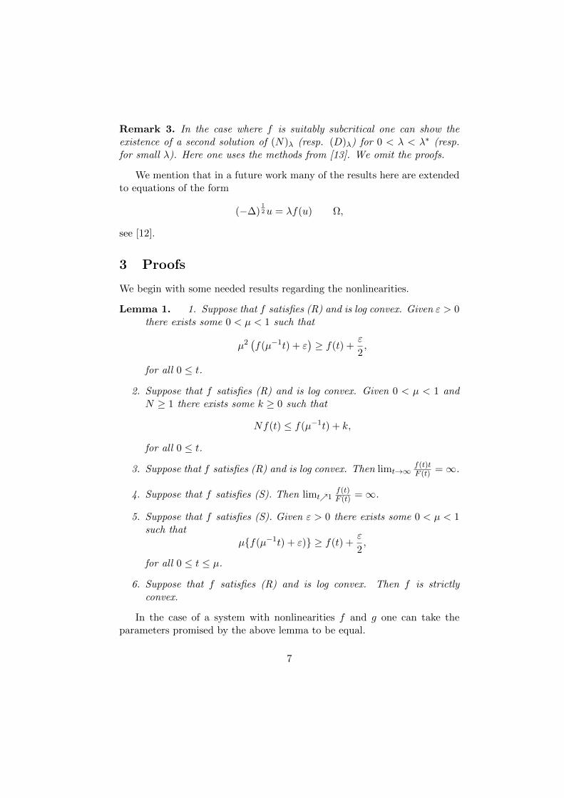
Remark 3. In the case where f is suitably subcritical one can show theexistence of a second solution of (N)λ (resp. (D)λ) for 0 < λ < λ∗ (resp.for small λ). Here one uses the methods from [13]. We omit the proofs.

We mention that in a future work many of the results here are extendedto equations of the form

(−∆)12u = λf(u) Ω,

see [12].

3 Proofs

We begin with some needed results regarding the nonlinearities.

Lemma 1. 1. Suppose that f satisfies (R) and is log convex. Given ε > 0there exists some 0 < µ < 1 such that

µ2(f(µ−1t) + ε

)≥ f(t) +

ε

2,

for all 0 ≤ t.

2. Suppose that f satisfies (R) and is log convex. Given 0 < µ < 1 andN ≥ 1 there exists some k ≥ 0 such that

Nf(t) ≤ f(µ−1t) + k,

for all 0 ≤ t.

3. Suppose that f satisfies (R) and is log convex. Then limt→∞f(t)tF (t) =∞.

4. Suppose that f satisfies (S). Then limt1f(t)F (t) =∞.

5. Suppose that f satisfies (S). Given ε > 0 there exists some 0 < µ < 1such that

µf(µ−1t) + ε) ≥ f(t) +ε

2,

for all 0 ≤ t ≤ µ.

6. Suppose that f satisfies (R) and is log convex. Then f is strictlyconvex.

In the case of a system with nonlinearities f and g one can take theparameters promised by the above lemma to be equal.

7

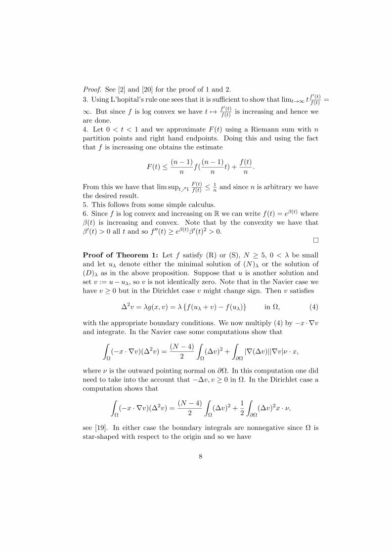
Proof. See [2] and [20] for the proof of 1 and 2.

3. Using L’hopital’s rule one sees that it is sufficient to show that limt→∞ tf ′(t)f(t) =

∞. But since f is log convex we have t 7→ f ′(t)f(t) is increasing and hence we

are done.4. Let 0 < t < 1 and we approximate F (t) using a Riemann sum with npartition points and right hand endpoints. Doing this and using the factthat f is increasing one obtains the estimate

F (t) ≤ (n− 1)

nf(

(n− 1)

nt) +

f(t)

n.

From this we have that lim supt1F (t)f(t) ≤

1n and since n is arbitrary we have

the desired result.5. This follows from some simple calculus.6. Since f is log convex and increasing on R we can write f(t) = eβ(t) whereβ(t) is increasing and convex. Note that by the convexity we have thatβ′(t) > 0 all t and so f ′′(t) ≥ eβ(t)β′(t)2 > 0.

Proof of Theorem 1: Let f satisfy (R) or (S), N ≥ 5, 0 < λ be smalland let uλ denote either the minimal solution of (N)λ or the solution of(D)λ as in the above proposition. Suppose that u is another solution andset v := u− uλ, so v is not identically zero. Note that in the Navier case wehave v ≥ 0 but in the Dirichlet case v might change sign. Then v satisfies

∆2v = λg(x, v) = λ f(uλ + v)− f(uλ) in Ω, (4)

with the appropriate boundary conditions. We now multiply (4) by −x ·∇vand integrate. In the Navier case some computations show that∫

Ω(−x · ∇v)(∆2v) =

(N − 4)

2

∫Ω

(∆v)2 +

∫∂Ω|∇(∆v)||∇v|ν · x,

where ν is the outward pointing normal on ∂Ω. In this computation one didneed to take into the account that −∆v, v ≥ 0 in Ω. In the Dirichlet case acomputation shows that∫

Ω(−x · ∇v)(∆2v) =

(N − 4)

2

∫Ω

(∆v)2 +1

2

∫∂Ω

(∆v)2x · ν,

see [19]. In either case the boundary integrals are nonnegative since Ω isstar-shaped with respect to the origin and so we have

8

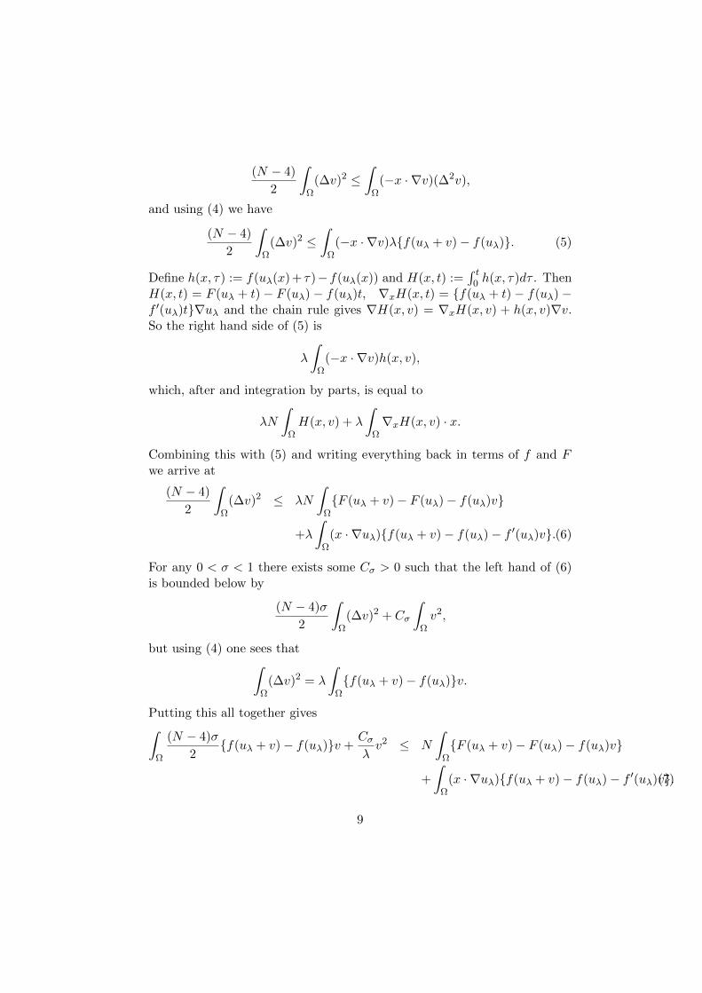
(N − 4)

2

∫Ω

(∆v)2 ≤∫

Ω(−x · ∇v)(∆2v),

and using (4) we have

(N − 4)

2

∫Ω

(∆v)2 ≤∫

Ω(−x · ∇v)λf(uλ + v)− f(uλ). (5)

Define h(x, τ) := f(uλ(x) + τ)−f(uλ(x)) and H(x, t) :=∫ t

0 h(x, τ)dτ . ThenH(x, t) = F (uλ + t)− F (uλ)− f(uλ)t, ∇xH(x, t) = f(uλ + t)− f(uλ)−f ′(uλ)t∇uλ and the chain rule gives ∇H(x, v) = ∇xH(x, v) + h(x, v)∇v.So the right hand side of (5) is

λ

∫Ω

(−x · ∇v)h(x, v),

which, after and integration by parts, is equal to

λN

∫ΩH(x, v) + λ

∫Ω∇xH(x, v) · x.

Combining this with (5) and writing everything back in terms of f and Fwe arrive at

(N − 4)

2

∫Ω

(∆v)2 ≤ λN

∫ΩF (uλ + v)− F (uλ)− f(uλ)v

+λ

∫Ω

(x · ∇uλ)f(uλ + v)− f(uλ)− f ′(uλ)v.(6)

For any 0 < σ < 1 there exists some Cσ > 0 such that the left hand of (6)is bounded below by

(N − 4)σ

2

∫Ω

(∆v)2 + Cσ

∫Ωv2,

but using (4) one sees that∫Ω

(∆v)2 = λ

∫Ωf(uλ + v)− f(uλ)v.

Putting this all together gives∫Ω

(N − 4)σ

2f(uλ + v)− f(uλ)v +

Cσλv2 ≤ N

∫ΩF (uλ + v)− F (uλ)− f(uλ)v

+

∫Ω

(x · ∇uλ)f(uλ + v)− f(uλ)− f ′(uλ)v.(7)

9

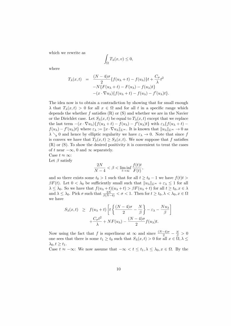
which we rewrite as ∫ΩTλ(x, v) ≤ 0,

where

Tλ(x, t) =(N − 4)σ

2f(uλ + t)− f(uλ)t+

Cσλt2

−NF (uλ + t)− F (uλ)− f(uλ)t−(x · ∇uλ)f(uλ + t)− f(uλ)− f ′(uλ)t.

The idea now is to obtain a contradiction by showing that for small enoughλ that Tλ(x, t) > 0 for all x ∈ Ω and for all t in a specific range whichdepends the whether f satisfies (R) or (S) and whether we are in the Navieror the Dirichlet case. Let Sλ(x, t) be equal to Tλ(x, t) except that we replacethe last term −(x · ∇uλ)f(uλ + t)− f(uλ)− f ′(uλ)t with ελf(uλ + t)−f(uλ)− f ′(uλ)t where ελ := ‖x ·∇uλ‖L∞ . It is known that ‖uλ‖L∞ → 0 asλ 0 and hence by elliptic regularity we have ελ → 0. Note that since fis convex we have that Tλ(x, t) ≥ Sλ(x, t). We now suppose that f satisfies(R) or (S). To show the desired positivity it is convenient to treat the casesof t near −∞, 0 and ∞ separately.Case t ≈ ∞:Let β satisfy

2N

N − 4< β < lim inf

t→∞

f(t)t

F (t),

and so there exists some t0 > 1 such that for all t ≥ t0 − 1 we have f(t)t >βF (t). Let 0 < λ0 be sufficiently small such that ‖uλ‖L∞ + ελ ≤ 1 for allλ ≤ λ0. So we have that f(uλ + t)(uλ + t) > βF (uλ + t) for all t ≥ t0, x ∈ λand λ ≤ λ0. Pick σ such that 2N

β(N−4) < σ < 1. Then for t ≥ t0, λ < λ0, x ∈ Ωwe have

Sλ(x, t) ≥ f(uλ + t)

[t

(N − 4)σ

2− N

β

− ελ −

Nuλβ

]+Cσt

2

λ+NF (uλ)− (N − 4)σ

2f(uλ)t.

Now using the fact that f is superlinear at ∞ and since (N−4)σ2 − N

β > 0one sees that there is some t1 ≥ t0 such that Sλ(x, t) > 0 for all x ∈ Ω, λ ≤λ0, t ≥ t1.Case t ≈ −∞: We now assume that −∞ < t ≤ t1, λ ≤ λ0, x ∈ Ω. By the

10

monotonicity and convexity of f we have the lower bound

Sλ(x, t) ≥ Cσt2

λ−NF (uλ + t)− F (uλ)− f(uλ)t

−f(uλ + t)− f(uλ)− f ′(uλ)t. (8)

Note that all terms except the first term grow at most linearly in t as t →−∞. Hence there exists some λ1 ≤ λ0 such that Sλ(x, t) > 0 for all −∞ <t ≤ −1, λ < λ1, x ∈ Ω. Note this step is not needed in the Navier case. Wenow consider the final case.Case t ≈ 0:By Taylor’s Theorem there exists some C1 > 0 such that

|F (uλ + t)−F (uλ)− f(uλ)t| ≤ C1t2, |f(uλ + t)− f(uλ)− f ′(uλ)t| ≤ C1t

2,

for all −1 ≤ t ≤ t1, λ < λ0, x ∈ Ω. Substituting this into (8) and taking λ1

smaller if necessary we have that Sλ(x, t) > 0 for all 0 6= t ∈ [−1, t1], λ <λ0, x ∈ Ω.We now assume that f satisfies (S). Our starting point is (7) and we takeσ = 1

2 . Again we break the interval for t into 3 regions (but now the regionsdepends on x): t ∈ (1 − ε − uλ(x), 1 − uλ(x)) (where ε > 0 is small),t ∈ (−1, 1 − ε − uλ(x)) and t ∈ (−∞,−1]. We argue as before and we useLemma 1, 4 to get the desired positivity on the first region. For the otherregions we argue as before. We omit the details.

2

Proof of Theorem 2: Let Ω be a domain in RN with N ≥ 3 and whichis star shaped with respect to the origin. Our goal it to show that theonly solution of (P )λ,γ for (λ, γ) ∈ Q with λ2 + γ2 small is the minimalsolution. By a symmetry argument it is sufficient to prove the result for0 ≤ γ ≤ λ. If γ = λ then (P )λ,γ reduces to the scalar equation, see (9),and we have uniqueness. Instead of using parameters (λ, γ) we prefer to use(λ, γ) = (λ, σλ) and after considering the above comments we restrict ourattention to 0 < σ < 1. So with this notation we let (uλ,σ, vλ,σ) denote theminimal solution of (P )λ,λσ where 0 < λ and 0 < σ < 1. Let wλ denotethe minimal solution associated with (Q)λ in the case of f(t) = et and notethat (wλ, wλ) is a supersolution of (P )λ,λσ for 0 < σ < 1 and hence we seethat (uλ,σ, vλ,σ) → 0 in L∞(Ω) × L∞(Ω) as λ 0 uniformly in 0 < σ < 1.Using elliptic regularity we have (uλ,σ, vλ,σ)→ 0 in C1(Ω)×C1(Ω) as λ 0uniformly in 0 < σ < 1. This shows that supΩ(|x · ∇uλ,σ|+ |x · ∇vλ,σ| → 0as λ 0 uniformly in 0 < σ < 1.

11

Let (u, v) denote a second solution of (P )λ,σλ and set uo := u − uλ,σ,vo := v − vλ,σ. Note these are both nonnegative and not identically zero.We first obtain the pointwise estimates:

i) v ≤ u, ii) σu ≤ v, iii) σuo ≤ vo, iv) vo ≤ uo, (9)

where for i)- iii) there are no parameter restrictions but in iv) the inequalitywill only hold for 0 < λ < λ1 and 0 < σ < 1 where λ1 > 0 is small.Note that since (u, v) is any solution that i) and ii) also hold for the minimalsolution. We now proof these. i) First note that we have −∆(u − v) =λ(ev − σeu). Multiply this by (u− v)− and integrate over Ω to see that

−∫

Ω|∇(u− v)−|2 = λ

∫Ω

(ev − σeu)(u− v)−,

and note the right hand side is nonnegative, hence the left hand side is zeroand we have (u− v)− = 0 a.e..ii) Note that−∆(v−σu) = λσ(eu−ev) which is nonnegative after consideringi) and after an application of the maximum principle we see that v ≥ σu.iii) A computation shows that (uo, vo) satisfy

−∆uo = λevλ,σ(evo − 1) Ω, (10)

−∆vo = σλeuλ,σ(euo − 1) Ω, (11)

with zero Dirichlet boundary conditions. Set Ω0 := x ∈ Ω : vo(x) < σuo(x).To show iii) we need to show that Ω0 is empty, so towards a contradictionwe assume its not. Note that in Ω0 we have

−∆(vo − σuo) = λσ euλ,σ(euo − 1)− evλ,σ(evo − 1)≥ λσ evλ,σ(euo − 1)− evλ,σ(evo − 1) by i)

= σλevλ,σ(euo − evo)≥ σλevλ,σ(e

voσ − evo)

where the last line follows since we are in Ω0. Now since σ < 1 one sees thefinal quantity is nonnegative and hence we have that −∆(vo − σuo) ≥ 0 inΩ0. Applying the maximum principle we have vo ≥ σuo in Ω0, which givesus the desired contradiction.iv) A computation shows that

−∆(uo − vo) = λevλ,σ(evo − 1)− σλeuλ,σ(euo − 1)

≥ λeσuλ,σ(evo − 1)− σλeuλ,σ(euo − 1) (12)

12

since vλ,σ ≥ σuλ,σ.A calculus argument shows that there exists some 0 < t0 small such that

one haseσt ≥ σet ∀0 ≤ t ≤ t0, ∀0 < σ < 1. (13)

Let 0 < λ1 be sufficiently small such that for all 0 < λ < λ1 one has that‖uλ,σ‖L∞ < t0 for all 0 < σ < 1. We now take 0 < λ < λ1 and note that wehave eσuλ,σ ≥ σeuλ,σ . Substituting this into (12) gives

−∆(uo − vo) ≥ λσeuλ,σ(evo − euo)

which re-arranges to

−∆(uo − vo) + λσuuλ,σc(x)(uo − vo) ≥ 0,

where c(x) = euo−evouo−vo ≥ 0 and is smooth. The maximum principle now gives

the desired result and we have completed the proofs of i) - iv). We nowreturn to proving uniqueness. Let 0 < λ < λ1 and 0 < σ < 1. Multiply (10)by −x · ∇vo and (11) by −x · ∇uo and integrate to obtain∫

Ω∆uo(x · ∇vo) = λN

∫Ωevλ,σ(evo − vo − 1)

+λ

∫Ωevλ,σ(x · ∇vλ,σ)(evo − vo − 1) (14)

∫Ω

∆vo(x · ∇uo) = λNσ

∫Ωeuλ,σ(euo − uo − 1)

+λσ

∫Ωeuλ,σ(x · ∇uλ,σ)(euo − uo − 1). (15)

A computations shows that ∆(x ·∇vo) = 2∆vo +x ·∇(∆vo). Using this anda integration by parts shows that

∫Ω

∆uo(x ·∇vo)+∆vo(x ·∇uo) = (N −2)

∫Ω∇uo ·∇vo+

∫∂Ω|∇uo||∇vo|x ·ν.

(16)Note for the boundary term we have used the fact that uo, vo ≥ 0 in Ω.Adding (14) and (15) and using (16) gives

13

(N − 2)

∫Ω∇uo · ∇vo ≤ λN

∫Ωevλ,σ(evo − vo − 1)

+λ

∫Ωevλ,σ(x · ∇vλ,σ)(evo − vo − 1)

+λNσ

∫Ωeuλ,σ(euo − uo − 1)

+λσ

∫Ωeuλ,σ(x · ∇uλ,σ)(euo − uo − 1). (17)

Now we know that −∆uo,−∆vo ≥ 0 and we also have σuo ≤ vo ≤ uo.From this we see that

∫Ω∇uo · ∇vo =

∫Ω

(−∆uo)vo ≥ σ∫

Ω|∇uo|2 ≥ σλ1(Ω)

∫Ωu2o, (18)

and similarly one shows∫Ω∇uo · ∇vo ≥ λ1(Ω)

∫Ωv2o , (19)

where λ1(Ω) denotes the first eigenvalue of −∆ in H10 (Ω). Using (10) and

(11) one also sees that

λ

∫Ωevλ(evo − 1)vo =

∫Ω∇uo · ∇vo = λσ

∫Ωeuλ(euo − 1)uo. (20)

The idea is to now break the left hand side of (17) into four equal partsand use (18), (19) and (20) to rewrite (17). We now take 0 < λ < λ1

sufficiently small such that euλ,σ , evλ,σ < 2 for all 0 < σ < 1. Doing this weobtain an inequality of the form∫

Ωσ

u2o

λ+ (euo − 1)uo − C(euo − uo − 1)

+

v2o

λ+ (evo − 1)vo − C(evo − v0 − 1)

dx ≤ 0

(21)where C = C(N) > 0. One easily sees that for 0 < λ sufficiently small thatthe integrand in (21) is positive on (uo, vo) : uo, vo ≥ 0\(0, 0). Hencewe have uo = vo = 0 and so (u, v) = (uλ,σ, vλ,σ).

2

Proof of Theorem 3; part 1. We first show that the extremal solutionis a weak solution. Let (u∗, v∗) denote the extremal solution corresponding

14

to the parameters (λ∗, γ∗). Using the techniques from [26] one sees that(u∗, v∗) is a weak solution of (P )λ∗,γ∗ except for possibly the integrabilityconditions. To obtain these we obtain estimates on the minimal solutionsalong the ray through origin and through (λ∗, γ∗). Let (λ, γ) lie on this rayand let (u, v) denote the minimal solution of (P )λ,γ . Multiply −∆u = λf(v)by −x · ∇v and −∆v = γg(u) by −x · ∇u and add the inequalities andintegrate over Ω to arrive at∫

Ωx · ∇v∆u+ x · ∇u∆v =

∫Ωλf(v)(−x · ∇v) + γg(u)(−x · ∇u),

and arguing as in (14), (15) and (16) one sees that we have

(N − 2)

∫Ω∇u · ∇v ≤ λN

∫ΩF (v) + γN

∫ΩG(u).

Now using the equation for (u, v) we see that∫Ω

λ(N − 2)

2f(v)v +

γ(N − 2)

2g(u)u ≤

∫ΩλNF (v) + γNG(u).

From Lemma 1 we see that f(t)t dominates F (t) for t near ∞ (resp. near1) in the case where f satisfies (R) and is log convex (resp. f satisfies (S)).One has the same for g and G. From this we conclude that we have uniformbounds on

∫Ω f(v)v and

∫Ω g(u)u along the given ray and so passing to

limits we have v∗f(v∗), u∗g(u∗) ∈ L1(Ω) and we also have the desired H10 (Ω)

bound.We now show that the extremal solution is the unique solution. Assume

that 0 < σ < ∞ is such that γ∗ = σλ∗ and that (u, v) is a second weaksolution of (P )λ∗,γ∗ . For simplicity we assume that λ∗ = 1. By the mini-mality of the extremal solution we see that (u, v) ≥ (u∗, v∗) a.e. in Ω andwe have that u 6= u∗ and v 6= v∗. We now separate our argument into thetwo different classes of nonlinearites f and g we consider.

Case f and g satisfy (R) and are log convex. We now assume that fand g satisfy (R) and are log convex. Define

z1 :=u∗ + u

2, z2 :=

v∗ + v

2,

and note that z1 and z2 are weak solutions of

−∆z1 = f(z2) + h1(x), −∆z2 = σg(z1) + σh2(x), Ω,

15

with z1 = z2 = 0 on ∂Ω where we define hi in a moment.Define Ω1 = x ∈ Ω : v(x), v∗(x), u(x), u∗(x) ∈ R and note that Ω\Ω1 is aset of measure zero. We define

h1(x) =f(v∗) + f(v)

2− f(

v∗ + v

2) x ∈ Ω1,

h2(x) =g(u∗) + g(u)

2− g(

u∗ + u

2) x ∈ Ω1,

and we set both to be zero otherwise. Note that since f and g are convex wehave that 0 ≤ hi a.e. in Ω and since (u, v) and (u∗, v∗) are weak solutionswe have hi ∈ L1(Ω). Since f and g are strictly convex (either by hypothesisor by Lemma 1, 6) and so we have hi different from zero on a set of positivemeasure. Let χi be weak solutions of −∆χ1 = h1 and −∆χ2 = σh2 in Ωwith zero boundary conditions and let −∆φ = 1 in Ω with φ = 0 on ∂Ω. ByHopf’s Lemma there is some small ε > 0 such that χ1 ≥ εφ and χ2 ≥ εσφin Ω. We now set

τ1 := z1 + εφ− χ1, τ2 := z2 + σεφ− χ2,

and note that τi ≤ zi in Ω. A computation shows that τ1 and τ2 are weaksolutions of −∆τ1 = f(z2) + ε in Ω and −∆τ2 = σ(g(z1) + ε) in Ω withτi = 0 on ∂Ω. Since zi ≥ τi one sees that τi are weak supersolutions, in asuitable sense (see the proof of the claim), of −∆τ1 ≥ f(τ2) + ε in Ω and−∆τ2 ≥ σ(g(τ1) + ε) in Ω with τi = 0 on ∂Ω. We now use the followingclaim which we prove in a moment.Claim: There exists 0 ≤ wi smooth such that

−∆w1 = f(w2) +ε

2, −∆w2 = σ(g(w1) +

ε

2) Ω,

with wi = 0 on ∂Ω. Let wi be as in the claim and pick α > 0 but sufficientlysmall such that αw1 ≤ εφ

2 and αw2 ≤ σεφ2 in Ω, which is not an issue since

wi is smooth. Set w1 = w1 +αw1− εφ2 and w2 = w2 +αw2− σεφ

2 . Note thatwi ≤ wi in Ω and also note that a computation shows that

−∆w1 ≥ (1 + α)f(w2), −∆w2 ≥ (1 + α)σg(w1) Ω,

where wi = 0 on ∂Ω. The maximum principle shows that wi ≥ 0. Now oneuses a standard iteration argument to obtain a bounded solution, which issmooth after applying standard elliptic regularity theory, to (P )1+α,σ(1+α)

which contradicts the fact that we assumed λ∗ = 1. To finish the proof weneed only prove the claim and for this we switch notation slightly so as to cut

16

down on the indices. Suppose that ε > 0 and we have 0 ≤ u0, v0 ∈ L1(Ω) areweak solutions of −∆u0 = k0(x) and −∆v0 = k1(x) in Ω with u0 = v0 = 0on ∂Ω where 0 ≤ ki ∈ L1(Ω) and k0(x) ≥ f(v0)+ε and k1(x) ≥ σg(u0)+εin Ω. (I am using this somewhat restrictive notion of a weak supersolutionsince this is sufficient for our needs; also note we are taking u0 = τ1 andv0 = τ2). To prove the claim we need to now show the existence of boundedsolutions of −∆u = f(v) + ε

2 and −∆v = σ(g(u) + ε2) in Ω with u = v = 0

on ∂Ω. Let 0 < µ < 1 be as promised from Lemma 1, 1 and then let k befrom 1 (ii) of the same lemma. We let ui and vi for i = 1, 2, 3 denote weaksolutions of

−∆u1 = µ(f(v0) + ε), −∆v1 = µσ(g(u0) + ε) Ω,

−∆u2 = µ(f(v1) + ε), −∆v2 = µσ(g(u1) + ε) Ω,

−∆u3 = µ(f(v2) + ε), −∆v3 = µσ(g(u2) + ε) Ω,

all with zero Dirichlet boundary conditions. By the weak maximum principlewe have that 0 ≤ u3 ≤ u2 ≤ u1 ≤ µu0 and 0 ≤ v3 ≤ v2 ≤ v1 ≤ µv0 in Ω.Let −∆φ = 1 in Ω with φ = 0 on ∂Ω. Let T > 0 which we pick later. Notethat

−∆(u1 + Tφ) = T + µ(f(v0) + ε)

≥ T + µ(f(v1

µ) + ε)

≥ T + µ(Nf(v1)− k + ε)

= T + µε− µk −Nεµ+N(µf(v1) + µε)

= T + µε− µk −Nεµ+N(−∆u2)

and so if we take T big enough such that T + µε − µk −Nεµ ≥ 0 then wehave that Nu2 ≤ u1 + Tφ in Ω. A similar calculation shows that

−∆(v1 + Tφ) ≥ T + µσε− µσk −Nµσε+N(−∆v2) Ω,

and so by taking T larger if necessary we also have that Nv2 ≤ v1 +Tφ in Ω.Now since f and g are log convex we can write f(t) = eγ1(t) and g(t) = eγ2(t)

where γi is convex and increasing with γi(0) = 0. So we have that

f(v2) ≤ eγ1(v1+TφN

),

and note that

γ1(v1 + Tφ

N) = γ1(

1

Nv1 + (1− 1

N)

Tφ

(N − 1))

≤ γ1(v1)

N+ (1− 1

N)γ1(

Tφ

(N − 1))

17

and from this we obtain that

f(v2)N ≤ eγ1(v1)e(N−1)γ1( TφN−1

) ≤ f(v0)e(N−1)γ1( TφN−1

),

which shows that f(v2) ∈ LN (Ω). A similar calculation shows that g(u2) ∈LN (Ω) and hence by elliptic regularity theory we have that u3, v3 are boundedand note that since u3 ≤ u2 and v3 ≤ v2 we see that they satisfy −∆u3 ≥µ(f(v3) + ε) and −∆v3 ≥ σµ(g(u3) + ε) in Ω and we can apply a standarditeration argument to obtain smooth solutions u and v of −∆u = µ(f(v)+ε)and −∆v = σµ(g(u) + ε) in Ω with u = v = 0 on ∂Ω. We now set δ1 = µuand δ2 = µv. Then a computation shows that

−∆δ1 = µ2(f(v) + ε) = µ2(f(δ2

µ) + ε) ≥ f(δ2) +

ε

2Ω,

where the last inequality follows from Lemma 1, 1. A similar calculationshows that

−∆δ2 ≥ σ(g(δ1) +ε

2) Ω,

and we now obtained the desired result after a standard iteration argument.

Case f and g satisfy (S). We now assume that f and g satisfy (S).Everything carries through as in the previous case except for the proof ofthe Claim. Suppose that we have weak supersolutions (u, v) of

−∆u ≥ f(v) + ε, −∆v ≥ σ(g(u) + ε) Ω,

with Dirichlet boundary conditions. Let 0 < µ < 1 be as promised fromLemma 1, 5. Set u = µu and v = µv. The first thing to notice is thatu, v ≤ µ a.e. in Ω. A computation and Lemma 1, 5, show that (u, v) is aweak supersolution (but bounded away from 1) of

−∆u ≥ f(v) +ε

2, −∆v ≥ σg(u) +

ε

2, Ω

and so we can now apply a monotone iteration to obtain the desired result.This completes the proof of the of Theorem 3 part 1.

2

Proof of Theorem 3; part 2. It is known that u∗ is a weak solutionof (N)λ∗ see [2]. In fact the extremal solution enjoys the added regularity,f(u∗) ∈ L2(Ω), see [11]. We now show that u∗ is the unique weak solutionof (N)λ∗ and the proof is very similar to the proof of part 1 of the currenttheorem and so we will be somewhat brief. If no boundary conditions are

18

given in the following pde’s then it is understood they satisfy Navier bound-ary conditions. We suppose that u is a second weak solution of (N)λ∗ andfor simplicity we assume that λ∗ = 1. By the minimality of u∗ we havethat u∗ ≤ u a.e. in Ω and they differ on a set of positive measure. Setz := u∗+u

2 and note that z is a weak solution of ∆2z = f(z) + h(x) in Ωwhere h(x) = 2−1f(u∗) + f(u) − f(z) on Ω0 := x ∈ Ω : u∗(x), u(x) ∈ Rand where h(x) = 0 otherwise. Again we have |Ω\Ω0| = 0 and note that0 ≤ h on Ω. Since f is strictly convex we have that h is positive on set ofpositive measure. Let χ be a weak solution of ∆2χ = h in Ω and ∆2φ = 1 inΩ. By Hopf’s lemma (smooth out h if necessary) there is some ε > 0 suchthat −∆(χ−εφ) ≥ 0 in Ω and so the maximum principle shows that χ ≥ εφin Ω. Set τ := z+ εφ−χ and note that τ ≤ z a.e. in Ω. Also note that τ isa weak solution of ∆2τ = f(z) + ε in Ω and so τ ≥ 0 a.e. in Ω. Since z ≥ τwe see that τ is a weak supersolution of ∆2τ ≥ f(τ) + ε in Ω.Claim: there exists some smooth function 0 < w such that ∆2w = f(w) + ε

2in Ω.Take α > 0 but small enough such that αw ≤ εφ

2 in Ω. Set w = w+αw− εφ2

and note that w ≤ w. Then we see that w satisfies ∆2w ≥ (1 +α)f(w) in Ωand so w ≥ 0 in Ω. Using the usual iteration argument shows the existenceof a smooth solution to ∆2w = (1 + α)f(w) in Ω which contradicts the factthat λ∗ = 1. The only thing left to show is the claim. The proof is verysimilar to the proof of the analogous claim in part 1, so we omit the details.

2

References

[1] G. Arioli, F. Gazzola, H.-C. Grunau, and E. Mitidieri, A semilinearfourth order elliptic problem with exponential nonlinearity, SIAM J.Math. Anal., 36 (2005), pp. 12261258.

[2] E. Berchio and F. Gazzola, Some remarks on biharmonic elliptic prob-lems with positive, increasing and convex nonlinearities, ElectronicJournal of Differential Equations, Vol. 2005(2005), No. 34, pp. 120.

[3] T. Boggio, Sulle funzioni di Green dordine m, Rend. Circ. Mat. Palermo(1905), 97-135.

[4] H. Brezis, T. Cazenave, Y. Martel, A. Ramiandrisoa; Blow up for ut −∆u = g(u) revisited, Adv. Diff. Eq., 1 (1996) 73-90.

19

[5] H. Brezis and L. Vazquez, Blow-up solutions of some nonlinear ellipticproblems, Rev. Mat. Univ. Complut. Madrid 10 (1997), no. 2, 443–469.

[6] X. Cabre, Regularity of minimizers of semilinear elliptic problems up todimension four, Comm. Pure Appl. Math. 63 (2010), no. 10, 1362-1380.

[7] X. Cabre and A. Capella, Regularity of radial minimizers and extremalsolutions of semilinear elliptic equations, J. Funct. Anal. 238 (2006),no. 2, 709–733.

[8] D. Cassani, J.M. do O and N. Ghoussoub, On a fourth order ellipticproblem with a singular nonlinearity. Adv. Nonlinear Stud. 9 (2009),no. 1, 177-197.

[9] L.B. Chaabane, On the extremal solutions of semilinear elliptic prob-lems, Abstr. Appl. Anal. Volume 2005, Number 1 (2005), 1-9.

[10] C. Cowan, Regularity of the extremal solutions in a Gelfand systemproblem, Advanced Nonlinear Studies, Vol. 11, No. 3 , p. 695 Aug.,2011.

[11] C. Cowan, P. Esposito and N. Ghoussoub, Regularity of extremal solu-tions in fourth order nonlinear eigenvalue problems on general domains.Discrete Contin. Dyn. Syst. 28 (2010), no. 3, 10331050.

[12] C. Cowan and M. Fazly, Uniqueness of solutions for a nonlocal ellipticeigenvalue problem, Math. Res. Lett. 19 (2012), no. 03, 613-626.

[13] M.G. Crandall and P.H. Rabinowitz, Some continuation and variationmethods for positive solutions of nonlinear elliptic eigenvalue problems,Arch. Rat. Mech. Anal., 58 (1975), pp.207-218.

[14] J. Davila, L. Dupaigne, I. Guerra and M. Montenegro, Stable solutionsfor the bilaplacian with exponential nonlinearity, SIAM J. Math. Anal.39 (2007), 565-592.

[15] J. Dolbeault, R. Stanczy, Non-existence and uniqueness results for su-percritical semilinear elliptic equations. Ann. Henri Poincar 10 (2010),no. 7, 13111333,

[16] P. Esposito and N. Ghoussoub, Uniqueness of solutions for an ellip-tic equation modeling MEMS. Methods Appl. Anal. 15 (2008), no. 3,341353,

20

[17] P. Esposito, N. Ghoussoub and Y. Guo, Compactness along the branchof semi-stable and unstable solutions for an elliptic problem with a sin-gular nonlinearity, Comm. Pure Appl. Math. 60 (2007), 1731–1768.

[18] N. Ghoussoub and Y. Guo, On the partial differential equations of elec-tro MEMS devices: stationary case, SIAM J. Math. Anal. 38 (2007),1423-1449.

[19] T. Hashimoto, Existence and nonexistence of nontrivial solutions ofsome nonlinear fourth order elliptic equations Proceedings of thefourth international conference on dynamical systems and differentialequaions, May 24 27, 2002, Wilmington, NC, USA, pp 393-402.

[20] X. Luo, Uniqueness of weak extremal solution to biharmonic equationwith logarithmically convex nonlinearities, Journal of PDEs 23 (2010)315-329.

[21] Y. Martel, Uniqueness of weak extremal solutions of nonlinear ellipticproblems, Houston J. Math. 23 (1997), no. 1, p. 161168.

[22] J. McGough, On solution continua of supercritical quasilinear ellipticproblems. Differential Integral Equations 7 (1994), no. 5-6, 14531471.

[23] J. McGough, J. Mortensen, Pohozaev obstructions on non-starlikedomains. Calc. Var. Partial Differential Equations 18 (2003), no. 2,189205.

[24] J. McGough, J. Mortensen, C. Rickett and G. Stubbendieck, Domaingeometry and the Pohozaev identity. Electron. J. Differential Equations2005, No. 32, 16 pp.

[25] F. Mignot, J-P. Puel; Sur une classe de problemes non lineaires avecnon linearite positive, croissante, convexe, Comm. Partial DifferentialEquations 5 (1980) 791-836.

[26] M. Montenegro, Minimal solutions for a class of elliptic systems, Bull.London Math. Soc.37 (2005) 405-416.

[27] G. Nedev, Regularity of the extremal solution of semilinear elliptic equa-tions, C. R. Acad. Sci. Paris Sr. I Math. 330 (2000), no. 11, 997–1002.

[28] R. Schaaf, Uniqueness for semilinear elliptic problems: supercriti-cal growth and domain geometry, Adv. Differential Equations, 5:1012(2000), pp. 12011220.

21

[29] K. Schmitt, Positive solutions of semilinear elliptic boundary valueproblems, Topological methods in differential equations and inclusions(Montreal, PQ, 1994), NATO Adv. Sci. Inst. Ser. C Math. Phys. Sci.,vol. 472, Kluwer Academic Publishers, Dordrecht, 1995, pp. 447-500.

22