>»ί· ili:, ϊ., 1·«γ4 - thesis.bilkent.edu.tr

>»ί· ili:, ϊ . ?, 1·« γ4 J -/('.i.Ä -t Vt-?·*· ;-u.іЛ. . c!. .·;, ·, β*ι / .„»iç, .■ ; · :.■ _ ~ .*■ ν ·

·.■ Τ· .«κ. •».·;Ι. .V ί J

■Mr ·■ -···;.::

3S5J* S 4 ' ^

SHORT- AND LONG-TERM LINKS AMONG

EUROPEAN AND US STOCK MARKETS

A THESISSUBMITTED TO THE DEPARTMENT OF MANAGEMENT

AND THE GRADUATE SCHOOL OF BUSINESS ADMINISTRATIONOF BILKENT UNIVERSITY

IN PARTIAL FULFILLMENT OF THE REQUIREMENTS FOR THE DEGREE OF

MASTER OF BUSINESS ADMINISTRATION

By ^

ROBERT-JAN GERRITS

June, 1995

Н6

t. о 5 3 8 3 8

I certify that 1 have read this thesis and that in my opinion it is fully adequate, in scope

and in quality, as a thesis for the degree of Master of Business Administration.

Assist. Prof Avse YIJCF,

1 certify that 1 have read this thesis and that in my opinion it is fully adequate, in scope


A.ssist. Prof Can S. MI JOAN

1 certify that 1 have read this thesis and that in my opinion it is fully adequate, in scope


Assist. Prof Ashok THAMPY

Approved by Dean of the Graduate School of Business Administration

Prof Dr. Siihidev TOGAN

(1

ABSTRACT

SHORT- AND LONG-TERM LINKS AMONG

EUROPEAN AND US STOCK MARKETS

Robert-Jan Gerrits

M.B.A.

Supervisor: Prof. Ayse Yüce

June, 1995

Recently, national economies are becoming more internationalized because of

increased trade and more cooperation between national governments to remove the

barriers to free flow of goods, services, and financial, physical and human capital. The

relationship between equity markets in various countries have been extensively

examined in the literature. This study tests the interdependence between stock prices

in Germany, the UK, the Netherlands and the US, using daily closing prices for the

period between March 1990 and October 1994. Results of the tests showed that the

US exerts a significant impact on the European markets. Moreover, the three

European markets influence each other in the short- and long-run. This result implies

that these markets move together. Therefore, diversification among those national

stock markets will not greatly reduce the portfolio risk without sacrificing expected

return.

ÖZET

AVRUPA VE AMERİKA BORSALARI ARASINDA KISA VE UZUN

DÖNEM BAĞLANTILAR

Robert-Jan Gerrits

M BA.

Tez Yöneticisi; Prof. Ayşe Yüce

Haziran, 1995

Son yıllarda eşya, hizmet, finansal, fiziksel ve insan sermayesinin akışını

serbestleştirmek amacıyla sınırları kaldırmak üzere ulusal hükümetler arasında artan

işbirliği ve artan ticaret, ulusal ekonomilerin giderek enternasyonel bir kimlik

kazanmalarına yol açmaktadır. Çeşitli ülkelerin borsaları arasındaki ilişki literatürde

geniş bir şekilde incelenmiştir. Bu çalışma ise Almanya, İngiltere, Hollanda ve

Amerika'daki hisse fiyatları arasındaki bağımlılığı. Mart 1990 - Ekim 1994 tarihleri

arasında günlük kapanış fiyatlarını kullanarak test etmektedir. Test sonuçlan

Amerika'nın Avrupa piyasaları üzerinde önemli bir etkisi olduğunu göstermektedir.

Bunun yanısıra, üç Avrupa borsası da kısa ve uzun dönemde birbirlerini etkilemektedir.

Böylece, değişik ülkelerin hisse senetlerine yatırım yapmak portföy riskini büyük

ölçüde azaltmayacaktır.

ACKNOWLEDGMENT

I would like to express my gratitude to Assist. Prof. Ayse Yüce for her guidance,

support and encouragement for the preparation of this thesis. I would like to thank my

other thesis committee members Assist. Prof Can S. Mugan and Assist. Prof Ashok

Thampy for their valuable comments and suggestions. I would also like to thank the

Department of Management of Bilkent University for providing me this MBA

education.

In addition, I would like to express my thanks to my colleagues for their comments

and support and my specials thanks to my friend Bilge Alp and my parents and

brother for their support and encouragement during my M.B.A. education.

Contents:

1. Introduction

2. Literature Review

3. Data

4.. Methodology

4.1 Stationarity4.2 Short- and Long-term Linkages

5. Empirical Results

5.1 Stationarity Properties of the Time Series5.2 Cointegration Tests5.3 Vector Error Correction

6. Conclusion

References

2

12

12

1215

19

192425

27

29

1

Appendix I: Appendix II: Appendix III: Appendix IV: Appendix V: Appendix VI: Appendix VII: Appendix VIII:

Correlograms for Amsterdam EOE Index Correlograms for New York Dow Jones Correlograms for London FT-100 Index Correlograms for Frankfurt Dax Index Statistical Properties of dLn(DAX) data Statistical Properties of dLn(AEX) data Statistical Properties of dLn(FT) data Statistical Properties of X and Ln(DJ) data

3233343536373839

1. Introduction

In the last 30 years there has been an increase in diversification at several levels in the

world economy. Large firms have discovered advantages in international diversification and haVe

diversified direct investments geographically and across industries to become today's

multinational corporations. Smaller investors and professional investment and pension fund

managers, who look after their interests, have also become aware of the potential benefits of

international diversification. Cross border investment continues its rapid worldwide growth as

investors are attracted by the potential opportunities for increased returns and diversification

benefits to be gained from an international approach to investment. In response to this

phenomenon, banks and financial institutions have multiplied the international products and

services they offer, while organized financial markets have tried to cope by adjusting products

procedures and trading times. Due to financial deregulation and advances in computer

technology, world stock markets have become more integrated. The globalization of markets and

economies have resulted in stronger linkages between the markets of the world.

However, at the heart of the concept of international diversification is the notion that

economic conditions and shareholders' returns in different (domestic and foreign) markets are

less than perfectly correlated. If this is indeed the case, it is possible to reduce portfolio risk

without sacrificing expected return by selecting individual securities in such a way that their risk

characteristics offset each other.

To examine long-term links and short-run causality for four different capital markets, the

subject of my thesis, I will use a vector error correction model. This paper discusses the

methodology that will be used to check for short- and long-term links among the markets and

will furthermore pay attention to the characteristics and the stationarity of the data-sets.

2. Literature Review

Recently, national economies are becoming more internationalized because of increased

trade and more cooperation between national governments to remove the barriers to free flow of

goods, services, and financial, physical and human capital. The relationships between equity

markets in various countries have been extensively examined in many prior empirical studies.

However, many early studies have made a strong case for international portfolio diversification.

The benefits of international diversification have been extensively documented (Solnik, 1988).

Such diversification allows to reduce the total risk of a portfolio while enhancing the

pfirformance opportunities.

The lack of interdependence across national stock markets has been presented as evidence

supporting the benefits of international portfolio diversification. In the causality literature.

Granger and Morgenstern (1970) use spectral analysis on weekly data for stock indices in eight

countries. Their empirical evidence shows few or no interrelationships between the stock markets

examined, except in the cases of the US-Holland and Germany-Holland. Agmon (1972) using

weekly or monthly return data, find no significant leads or lags among the common stocks of

Germany, Japan, the UK and the USA. Studies, such as Lessard (1976) and Jorion and Schwartz

(1986), using regression models to test for the existence but not the degree of market

segmentation, suggest that market segmentation does exist in some national equity markets.

The stock market crash of 1987 has provide new insights into the economic nature of

globalization of stock markets. Dwyer and Hafer (1988), using daily data for seven months

before and after the October 1987 crash, show no evidence that the levels of stock price indices

for the US, Japan, Germany and the UK are related. They report statistical evidence, however,

that the changes in the stock price indices in these four markets are generally related.

More recent studies, however, examining the stock price indices around the crash by Eun

and Shim (1989), von Furstenberg and Jeon (1989), and Bertera and Mayer (1990) report a

substantial amount of interdependence among national stock markets.

Eun and Shim (1989) investigate the international transmission mechanism of stock

market movements by estimating a nine-market VAR system, including the US, Japan, and Hong

Kong. The results show that innovations in the US are rapidly transmitted to the stock market in

Japan and Hong Kong market to be independent of one another.

Von Furstenberg and Jeon (1989) used daily data from 1986 to 1988 to analyze the

relationships for stock markets in London, Frankfurt, Tokyo and New York during and after the

October 1987 market crash. They use a four-variable VAR model for investigating the

interdependence of the four markets. They report that the degree of international co-movements

in stock price indices had increased significantly after the crash.

Bertera and Mayer (1990) examines the stock price indices and the structure of 23 stock

markets including Australia, Hong Kong, Malaysia, Mexico, Singapore, South Africa, New

Zealand, Japan, the US and some European countries around the crash of 1987. They compared

the size, trading volume and some trade characteristics and analyzed the interdependencies

between these markets. Their study showed that the correlations between all regions increased

and remained higher after the crash.

Many studies have been made to examine the international linkage between the US and

Japan. Gultekin et al. (1989), Becker et al. (1990), Hamao et al. (1990), Kasa (1991), and Smith

et al. (1993) find high correlations between the two markets with an asymmetric spillover effect

from the US to the Japanese market, while Smith et al. (1993) and Aggerwal and Park (1994),

however, find that US equity prices do not lead Japanese equity prices and state that gains from

international diversification are obtainable.

Gultekin et al. (1989) focus on Japan and the US to test the integration of capital markets.

Weekly stock returns calculated from daily closing prices of the markets are used for two sample

periods around the December 1980 liberalization in Japan: 1977 to 1980 and 1981 to 1984. To

test the hypothesis of market integration, an international version of a multifactor assets pricing

model is used. Using multifactor asset pricing models, they show that the price of risk in the US

and Japanese stock markets was different before, but not after, the liberalization. This evidence

supports the view that governments are the source of international capital market segmentation.

Becker et al. (1990) study the inter-temporal relation between the US and Japanese stock

markets for the period 1985-1988. They use daily opening and closing data the market indexes.

Correlations and regression are used for detection of lead-effects and determination of the

relation between the two markets. They find a high correlation between the open to close returns

for US stocks in the previous trading day and the Japanese equity market performance in the

current period. In contrast, the Japanese market has only a small impact on the US return in the

current period. In addition, there is no relation between the performance of the Japanese market

and the close to open return in the US. High correlations among open to close returns are a

violation of the efficient market hypothesis. However, profitable trading on Japanese market

based on the movements on New York stock exchange was not possible due to the high trading

costs in Japan.

Hamao et al. (1990) study the short-run interdependence of prices and price volatility

across three major international stock markets. Daily opening and closing prices of major stock

indexes for the Tokyo, London and New York stock markets are examined over the period 1985-

1988. The analysis utilizes the autoregressive conditionally heteroskedastic (ARCH) family of

statistical models to explore these pricing relationships. They find spillover effects from the US

and the UK stoek markets to the Japanese market. This effect shows an intriguing asymmetry:

while the volatility spillover effect on the Japanese market is significant, the spillover effects on

the other two markets are much weaker. Unexpected changes in foreign market indices are

associated with significant spillover effects on the eonditional mean of the domestic market for

both open-to-elose and close-to-open returns. For the elose-to-open returns, this effect on the

conditional mean is consistent with international financial integration, while the magnitude of

volatility spillover is generally much less.

Kasa (1991) present evidence concerning the number of eommon stoehastie trends in the

equity markets of the US, Japan, the UK, Germany, and Canada. Monthly and quarterly indices

data from 1974 through 1990 are used. Johansen’s tests (1990) and the present value model of ·

asset pricing are applied to the stock markets. The results indicate the presence of a single

common trend driving these countries’ stock markets. Estimates of the factor loadings suggest

that this trend is most important in the Japanese market and least important in the Canadian

market. These results imply that to investors with long holding periods the gains from

international diversification have probably been overstated in the literature. Specifically, the

presenee of a single common stochastic trend means that these markets are perfeetly correlated

over long (infinite) horizons.

In contrast with the previous studies. Smith et al. (1993) and Aggerwal and Park (1994)

find evidenee supporting the benefits of international portfolio diversifieation.

Smith et al. (1993) examine the possible market linkages using weekly returns from

markets in the US, the UK, West-Germany and Japan, during the 1979-1991 period. Granger

causality tests are applied to the weekly data. Evidence of Granger unidirectional causality

running from the US to the other countries immediately after the Oetober 1987 world-wide crash

is found. For the most part, this linkage appears to be short-lived, with the exception of the

linkage from the US to the German market. These are episodes of other countries Granger-

causing the US, but these are short-lived as well. Given the results, one can conclude that the

market crash in the US caused instability, which was transmitted to other major markets around

the world. Other than the crash period, there appears to be a lack of Granger causality from

market to market, except the US/German relationship. In terms of their aggregate returns data,

the results are consistent with the idea that gains from international diversification are obtainable,

for the most part, shocks from one market are not transmitted to other markets around the world.

Aggerwal and Park (1994) presents evidence of the international integration of the US

and Japanese equity markets. They used daily opening and closing prices of the stock markets

from 1987 to 1991. This paper accounts for the problem of non-synchronous trading associated

with the calculated spot opening value of the market index. This study find hat US equity prices

do not lead Japanese equity prices. Both US and Japanese opening equity prices reflect overnight

price changes in the other market.

The conflicting evidence leads naturally to the question why are there differences in

results? Meric and Meric (1989) analyze the inter-temporal stability of the matrix of correlation

coefficients among seventeen national stock markets (Spain, Singapore, Australia, the US,

Canada, Hong Kong, Italy, Norway, France the UK, Belgium, Austria, Germany, Switzerland,

Netherlands, Sweden and Japan). They use month-end closing stock market indices of the

different equity markets for the Box’s M methodology for the 1973-1987 period. They find

empirical evidence that diversification across countries results in greater risk reduction than

diversification across industries. Their inter-temporal stability tests indicate that, the longer the

time period considered, the better proxies ex post patterns of co-movement can be for the ex ante

co-movements of international stock markets. Their seasonality tests show that international

stock market co-movements are stable in the September-May period, but relatively unstable in

the May-September period.

European countries are also frequently examined for interdependencies between stock

exchange markets. Mathur and Subrahmanyam (1990), Arshanpalli and Doukas (1993), and

Malliaris and Urrutia (1994) have used the concept of Granger causality, and cointegration and

error-correction models to analyze the linkages and dynamic interactions among stock prices.

Mathur and Subrahmanyam (1990) discuss the interdependencies between the US and

Nordic stock markets. They used monthly stock price indices for the period between 1974 to

1985. The data was examined by applying the concept of Granger causality. They concluded that

the US market affected only one of the four Nordic markets (Denmark). However, a high

interdependence was observed between the Nordic markets and they concluded that it was

possible to earn extra returns by anticipating stock price changes in one market by observing the

changes in others.

Arshanapalli and Doukas (1993) use recent developments in the theory of cointegration to

study the linkages and dynamic interactions among stock prices in Germany, UK, France, Japan,

and the US, using daily closing data from 1980 to 1990. Cointegration and the error-correction

model is applied in this study. For the pre-crash period they find that France, Germany, and UK

stock markets are not related to the US stock market. For the post-crash period, however, their

results show that the three major European stock markets (i.e. Franc, Germany and UK) are

indeed strongly linked (cointegrated) with the US stock market. The US stock market is found to

have a substantial impact on the French, German and UK markets. Stock market innovations in

any of the three European stock markets have no impact on the US stock market. In addition,

they find no evidence of interdependence among stock price indices between US and Japan.

Furthermore, the results show that the US and Japan stock markets have drifted far away from

each other since the October crash. The pattern of interactions among France, Germany, UK, and

Japan suggests that Japanese stock market innovations are unrelated to the performance of the

major European stock markets.

Malliaris and Urrutia (1994) uses a vector error correcting (VEC) model to examine long

term and short-run causality for five major European capital markets: the UK, France, Italy,

Belgium and Germany, flie data consists of daily closing prices of the equity market indexes for

the time period 1989 through 1992. The empirical results of the VEC model show statistically

significant long-term links and short-term causal relationships. There is a two way long-term

relationship between each pair of European equity indexes. These findings show that these

markets are not independent but move together. They adjust to each other in the long-run and

they lead or lag each other in the short-run. The results imply limitations in the role of portfolio

diversification and confirm a high degree of integration among European equity markets.

Recently, considerable attention is given to possible linkages and interdependencies in

major Asian countries. Lee et al. (1990), Chan, Gup and Pan (1992), Chowdhury (1994), Rogers

(1994), and Kwan (1995), using cointegration tests and vector autoregression analyses, report

that international diversification in those countries can be effective.

Lee, Pettit, and Swankoski (1990) provides evidence on the issue of seasonal

characteristics of international equity markets through an analysis of stock market returns in

Hong Kong, Korea, Singapore, faiwan, and the US during 1980-1988. The results show that

important day-of-the-week effects can be identified in Hong Kong, Korea and Singapore.

Moreover, the returns indicate a significant amount of underlying independence between the

various equity markets studied, thus providing strong arguments for investor diversification

beyond country boundaries.

Chan, Gup and Pan (1992) analyzed stock prices in the US and major Asian countries

(Hong Kong, South Korea, Singapore, Taiwan) using daily and weekly data. First they tested

pairwise correlation among these markets. The obtained correlation coefficients were low

indicating that international diversification among these markets could be effective. Second, to

test for the random walk, they applied Perron-Phillips unit root tests. The null hypotheses for unit

roots in all markets were not rejected indicating the random walk behaviour of indices. Lastly,

they applied co-integration tests and no evidence for con-integration between these markets was

found. T hey concluded that international diversification among the tested markets will be

effective.

Chowdhury (1994) analyzes the relationship among the stock markets of Hong Kong,

Korea, Singapore, Taiwan, Japan and the US, using daily stock market indices at closing time

from 1986 to 1990. A six-variable vector autoregressive (VAR) model is used to investigate the

strength and persistence of the effects of shock or innovation in one market on the other markets

in the model. The results show that innovations in the US are rapidly transmitted to the stock

market in Japan and Hong Kong, whereas neither of these two markets can explain the US

market movements. Moreover, the results indicate that a significant link exists between the stock

markets of Hong Kong and Singapore and those of Japan and the US. On the other hand, the

markets with severe restrictions on cross-country investing, that is, Korea and Taiwan, are not

responsive to innovations in foreign markets. Finally, the US stock market influences but is not

influenced by the four Asian markets.

Rogers (1994) sheds light on the issue of international capital mobility by examining the

effectiveness of entry barriers to foreign investment in several stock markets (the US, Japan,

Germany, the UK, Mexico, Chile, Argentina, Taiwan, Korea and Thailand). The daily closing

data is analyzed over three different sub-periods: (1) before the 1987 crash, 1986-1987, (2)

immediately after the crash (first 95 days), and (3) well after the crash (months 9 to 18). A vector

autoregression (VAR) analysis is used for the markets during the three sub-periods. Co

movements between major and emerging market stock prices around the 1987 crash reveal a

relationship between foreign entry barriers and stock price transmission. For most countries,

individual market return volatility and price spillovers among markets increase immediately after

the crash. However, in markets with stiff entry barriers, volatility rises but there are no price

spillovers. Price-spillovers into emerging markets are found only from the US to Chile and

Thailand, the countries where the weakest entry barriers, but not from Japan or the US to Taiwan

or Korea. In addition, all of the major markets exhibit increased volatility and price spillovers.

The evidence that several emerging-market countries are poorly integrated financially with the

industrialized countries has important macroeconomic welfare implications.

Kwan et al. (1995) apply the Engle and Granger cointegration analysis and Granger

causality tests to monthly data of nine major stock market indices (Australia, Hong Kong, Japan,

Singapore, South Korea, Taiwan, the UK, the US and West-Germany) from 1982 to 1991 to

examine for causal links. The result of their pairwise and higher-order cointegration tests reveal

that international stock market indices are not weak-form efficient individually and collectively

in the long run. In addition, their ‘bivariate’ causality results indicate the existence of significant

lead-lag relationships between equity markets. The US stock market leads four markets:

Australia, Japan, Hong Kong and the UK. However, in regard to the US, the results suggest that

none of the other eight markets Granger-cause the US stock market.

Another group of studies have modified existing models and frameworks to analyze the

existence of short- or long-term linkages among national stock exchange markets.

Koutoulas and Kryzanowski (1994) have modified the domestic and international

arbitrage pricing theories (lAPT and APT models) to encompass the hypotheses that the

Canadian and global North American equity markets are completely or partly integrated

10

(segmented). For the period from March 1969 through March 1988 both models indicated that

the Canadian equity market is only partly integrated (or equivalently, partly segmented) with the

American equity market.

Ammer and Mei (1994) have developed a new framework for measuring financial and

real economic linkages between countries, using US and UK data from 1957 to 1989. They

employ a variant of the Campbell and Shiller log-linearization method. Both real and financial

linkages are found to be greater after the Bretton Woods currency arrangement was abandoned in

the early 1970s. A common interest rate news component accounts for only a small part of the

return covariance because of the lack of predictability of short-term real interest rates. In a further

application of their methodology, they find that both real and financial integration typically

contribute to the (consistently positive) correlations between the returns on national stock

markets. In most cases, news about future dividend growth in two countries is more highly

correlated than contemporaneous output measures. This suggest that there are lags in the

international transmission of real economic shocks.

The literature review has shown that there is conflicting evidence for possible

international stock market linkages. This report will make another contribution to the discussion

of the benefits of international portfolio diversification as a result of the lack of interdependence

across national stock markets. In this thesis, the linkages among stock prices in the stock

exchanges of Germany, Holland, the UK, and the US are studied, using daily closing data from

March 1990 through October 1994. Cointegration tests and the vector error correction model,

VEC, are used for the analysis of a possible existence of short- and long-term linkages among the

equity markets.

] 1

3. Data

The data used to investigate short-run and long-run interdependencies consist of the daily closing

prices for the following equity market indexes; London (FTSE 100 Price Index - FTSEIOO),

Frankfurt DAX, Amsterdam EOE, and New York (Dow Jones Industrial Average - DJIA). Daily

closing data for all four indices have been collected over the period beginning March 1, 1990 and

ending October 5, 1994. The sample consists of 1188 observations. When national stock

exchanges were closed due to national holidays, bank holidays or severe weather conditions, the

index level was assumed to remain the same as that on the previous trading day.

The Financial Times - Stock Exchange 100 Share (FTSE 100) Index represents 70 percent of the

equity capitalization of all United Kingdom equities. The Amsterdam European Options

Exchange (EOE) Index consists of 25 shares, representing 88% of the total market while the

Deutsche Aktien Index (DAX) in Frankfurt represents 60% of the equity capitalization of all

German Equities, consisting of 30 shares. The Dow Jones Industrial Average (DJIA), however, is

the average of 30 stocks in the NYSE, and represents only 22-25% of the total market.

4. Methodology

In this study, the methodology I use for common trends in international stock markets is based on

the vector error correction model, VEC. The first step in examining trends in international stock

markets is to test for stationarity of the time series.

4.1 Stationarity

A time series is stationary when its basic statistical properties remain constant over time. One

method of detecting non-stationarity in a time series is to examine the correlogram. If one notices

that the autocorrelations in the correlogram do not die down rapidly (say after the 5 or 6 lags).

12

then the time series is not stationary. Another way is to test for the presence of a unit root in the

country’s stock price series.

Dickey-Fuller Test

The unit root test is proposed by David Dickey (1981) and Wayne-Fuller (1981) for testing for

stationarity. The model used here is as follows. Let Y,, which is growing over time, be described

by the following equation:

Yi = A + B t + P Y u + C| (1)

whereYtABtPe,

: market index :drift variable : trend coefficient :time for t=0, ....,1485 : coefficient : error term

There are two possible explanations for the growing characteristic of Yt, namely, Yt has a

positive trend (B>0) and would be stationary after detrending. In this case, Yi could be used in a

regression. Another possibility is that Yi has been growing because it is a non-stationary series

with a positive drift (i.e. A>0, B=0, P=l). In this case, one would like to work with delta Yt.

Dickey and Fuller (1981) generated statistics in order to test for non-stationarity. The test

procedure is as follows (Kendall, 1990). Let Yt be described by the following unrestricted

equations;

with-constant, no-trend

(i) Yt - Yt-i = A + (P-l)Yt-i + I j LjdYt.j + et

with-constant, with-trend

(ii) Yt - Yt-i = A + Bt + (P-l)Yi-i + Ej LjdYt.j + Ct

(2)

(3)

13

The null hypothesis for each is

(i) Hq: Y( is a random walk plus drift, P=1

(ii) Hq: Yt is a random walk plus drift around a stochastic trend, P=1

and the restricted equation

Y , - Y , . , = A + Z jL jd Y ,.j + e, (B=0 and P=l) (4)

t-ratio

For each case i and the chosen lag order ] the following t-test statistic should be calculated:

ti(P,j) = [(P-l)/SE(P)]

where SE(P) refers to the standard error of parameter P.

F-test

The restricted and one of the unrestricted regressions should be runned and the F-ratio should be

calculated as follows:

F = (N-k)(ESSR - ESSurV{q(ESSuR)} (6)

whereNkqESS

number of observationsnumber of estimated parameters in unrestricted regression number of parameter restrictionssum of squared error residuals from restricted model (ESSr) and unrestricted models (ESSur)

Then, F- distributions calculated by Dickey and Fuller (1981) are used for testing the hypothesis

of a non-stationarity (i.e. (A, B, P) = (A, 0, 1)).

14

4.2 Short- and Long term linkages

The methodology used to examine short- and long term linkages among equity markets, is the

vector error correction model, VEC. The VEC model is based on the concept of causality in the

Granger sense and on the notion of cointegration.

a) Granger Causality Tests

When analyzing a vector of time series it is useful to ask if one group of series is generated

separately from another group. Two assumptions are made:

(i) The future cannot cause the past. Strict causality can only occur with the past causing the

future.

(ii) A cause contains unique information about an effect that is not available elsewhere.

Granger causality tests are used to examine causality in time series models. A series Xt causes

another series Yt if it seen that the series Xt has information helping to characterize future Y's

that is unique. More specific, X is said to cause Y if a coefficient aj is not zero in the following

equation:111 111

Y , = C , + 2 a , X , . , + 2 ; b i Y , _ j + e , (7)i=l i=l

Similarly, Y is said to cause X if some coefficient is not zero in equation (8):m 'll

X, = < t..+ £ a ,Y H + Z P jX ,- j+ ft (8)i = l .j=l

If X causes Y and also Y causes X, then there is said to be feedback. The test for causality is

based on an F-statistic that is computed by running the above regressions in both unconstrained

(full model) and constrained (reduced model) forms:

F = [ ® i ? “ l/[T S trl w

where SSEr and SSEj-are the sum of squares of the residuals of the reduced model and full model,

respectively, and m the number of lags and T the number of observations.

15

b) Cointegration Tests

Although individual series that contain stochastic trends are non-stationary in their levels, if the

stochastic trends are common across series there will be stationary linear combinations of the

levels. This phenomenon is known as co-integration.

A process Xi is said to be an integrated process, if it is generated by an equation of the form

ap(B)(l-B)dXt = bqfB)e, (10)

where e, is zero-mean white noise, a(B), b(B) are polynomials in B of orders p, q respectively

(a(B) being a stationary operator), and d is an integer. Such a process will be denoted Xj

~ARIMA(p, d, q) (autoregressive integrated moving average of order p, d, q) or X, ~ 1(d). If Xt

and Y( are a pair of 1(d) series, then it will be generally true that a linear combination, such as

Z, = X,-AYi (11)

will also be 1(d). However, it can happen that there exists a constant A such that Zt ~ I(d-b), b>0.

When this happens, the pair of variables Xi and Y( will be said to be co-integrated and denoted

(X,, Y|) ~ CI(d, b). When d=b=l and there exists an A such that Zt = Xt - AYt is stationary, i.e. Zt

~ 1(0) then it means that both series individually have extremely important long-run components,

but that in forming Zt these long-run components cancel out and vanish. Zt can now be

interpreted as the equilibrium error, that is, the extent to which the economy is out of

equilibrium. Engle and Granger suggest to estimate the value of A by running the regression:

X, =y+AY,-he, (12)

We can then calculate the values of Zt.

If two time series produce a stationary trend, then there exists an error correction representation,

which suggest that one stock price index can be used to forecast the other. In other words, the

existence of cointegration between two stock price indices implies that either one or both markets

are inefficient.

16

c) Vector Error Correction Model, VEC

By combining the causality and cointegration test it is possible to develop a model that allows to

test for both short-term and long-term relationships between the series Xt and Yt.· the vector error

correction model (VEC):A m m

Y, - Y„, = a. + a, Z,., + 2 ; c,(X,., - X ,.,,) + y ;d ,(Y,_J - Y,_j,) + s, (13)i = l .1=1

where Zi-i = X,_, - AY,_, as defined in (4).

The potential long-run and short-run impact of the series X on the series Y are in the VEC model

decomposed as follows:

• a long-run component, represented by the cointegration term aiZi-i, also known as the error-

correction term. The correction adjustments of Y( to a disequilibrium error from the previous

period Z(.i can spread over several periods of time, with the coefficient aj indicating the

speed of the correction mechanism.

• a short-run component, given by the summation terms in the right hand side of equation (13).

These two terms represent past changes in the variables X and Y and characterize the short-

run dynamics. Specifically, the first summation term in equation (13) gives the short-run

impact of X on Y.

Similarly, the potential long-run and short-run impact of the series Y on the series X can be

expressed in the VEC model as follows:

X, - X,., = tto + a, Zm + XKi (Y„, - Y,_i.,) + X Zj(X ,.j - X,_.,) + p, (14)i=l j=l

From equations (6) and (7) follows that:

• the series Xt and Yt are cointegrated when at least one of the coefficients of ai or 3] is

different from zero. In this case, Xt and Yt exhibit long-run comovements. The significance

and size of the error-correction terms ai and 3| essentially captures the single-period response

of the dependent variable to departures from equilibrium.

17

• there is a short-term relationship between the series Xt and Y( when at least one of the

coefficients of C| or k; is different from zero.

The error correction model has the standard interpretation: the change in Xt is due to the

immediate, short-run effect from the change in Yi and to last period’s error, Z^, which represents

the long-run adjustment to past disequilibrium. Hence, estimation of the error-correction

equations is also expected to provide evidence about the long-run relationship and the nature of

the adjustment process among national stock markets. Furthermore, the error-correction analysis

is fundamental for testing the cross-border market efficiency hypothesis since it describes the

long-run dynamic adjustment process between two stock exchange markets.

18

5. Empirical Results

In this chapter, the characteristics and the stationarity of the data sets will be discussed, by means

of data plots, correlograms and Dickey-Fuller test.

5.1. Stationarity Properties of the Time Series

a) Data plots and correlograms

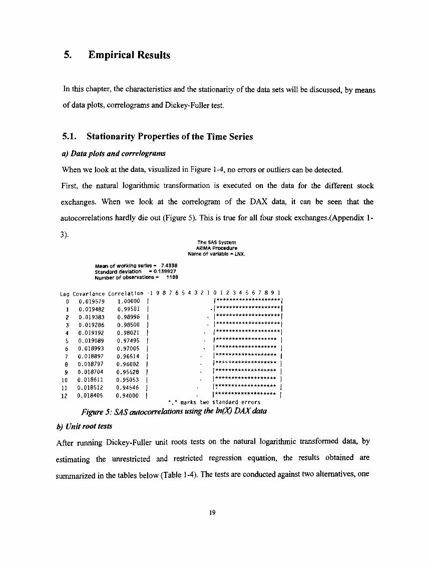
When we look at the data, visualized in Figure 1-4, no errors or outliers can be detected.

First, the natural logarithmic transformation is executed on the data for the different stock

exchanges. When we look at the correlogram of the DAX data, it can be seen that the

autocorrelations hardly die out (Figure 5). This is true for all four stock exchanges.(Appendix 1-

3).The SAS System

ARIMA Procedure Name of variable - LNX.

Mean of working series - 7.4338 Standard deviation "0.139927 Number of observations - 1188

-1 9 8 7 6 5 4 3 2 1 0 1 2 3 4 5 6 7 8 9 1j •ieir-k-k-k-k-k-k-kir-k-k-k-k'kir-k-k’k-k | j ★ ★ ★ ★ ★ ★ ★ ★ ★ ★ ★ ★ ★ ★ ★ ★ ★ ★ ★ ★ I I★ ★ ★ ★ ★ ★ ★ ★ ★ ★ *★ *★ *★ ★ ★ ★ ★ I I★ ★ ★ *★ ★ ★ ★ ★ ★ ★ *★ ★ ★ ★ *★ **I I★ ******★ ★ ★ ★ ★ ★ *★ ★ *★ ★ *I I j I*★ ★ ★ ★ ★ *★ *★ ★ ★ ***★ ★ ** I j j j ★ ★ y. >·**■*·★ ★ ★ ★ ★ ★ ★ ★ ★ ★ ★ ★ j j★ ★ ★ ★ ★ ★ ★ ★ ★ ★ ★ ★ ★ *★ ★ ★ ★ ★ j

I *★ **★ ★ ★ *■***★ ****★ *★ Imarks two standard errors

SAS autocorrelations using the ln()Q DAX data

b) Unit root tests

After running Dickey-Fuller unit roots tests on the natural logarithmic transformed data, by

estimating the unrestricted and restricted regression equation, the results obtained are

summarized in the tables below (Table 1-4). The tests are conducted against two alternatives, one

Lag Covariance Correlation0 0.019579 1.000001 0.019482 0.995012 0.019383 0.989963 0.019286 0.985004 0.019192 0.980215 0.019089 0.974956 0.018993 0.970057 0.018897 0.965148 0.018797 0.960029 0.018704 0.95528

10 0.018611 0.95053' l l 0.018512 0.9454612 0.018405 0.94000

Figure 5: SAS auta

19

New York Dow Jones

Date

Figure 1: Daily closing prices of New York DJIA, 01/03/90-05/10/94

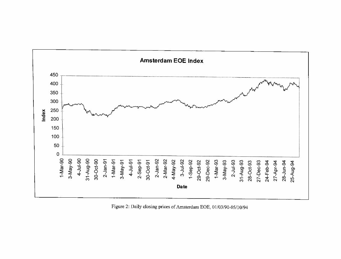
Amsterdam EOE Index

Date

Figure 2: Daily closing prices of Amsterdam EOE, 01/03/90-05/10/94

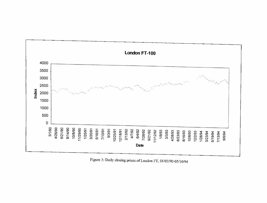
London FT-100

Figure 3: Daily closing prices of London FT, 01/03/90-05/10/94

Frankfurt DAX

X0)"öc

Date

Figure 4: Daily closing prices of Frankfurt DAX, 01/03/90-05/10/94

consistent with fluctuations around a constant mean, the other with stationary fluetuations around

a deterministic linear trend:

(i) Hq: Yt is a random walk plus drift, P=1

(ii) Hq.· Yi is a random walk plus drift around a stochastic trend, P=1

Table 1: Summary o f Dickey-Fuller and Phillips-Perron tests on Ln(AEX) dataL n (A E X ) D ick ey -F u ller

T est S ta tisticC ritica l va lu es at 10% level

P h illip s-P erro n T est S ta tistic

C ritica l va lu es at- 10% level

con stan t, no trend

t - s t a t i s t i c -0 .79907 -2 .57 -0 .52941 -2 .57

F - te s t 0.52165 3.78 0 .94452 3.78

con stan t, trend

t - s t a t i s t i c -3 .0430 -3.13 -1 .9164 -3 .13

F - te s t 4 .9 5 3 7 5.34 1.9789 5.34

Table 2: Summary o f Dickey-Fuller and Phillips-Perron tests on Ln(DJ) dataL n(D J) D ick ey -F u ller

T est S ta tistic

C ritica l va lu es at 10% level


C ritica l va lu es a t 10% level

co n sta n t, no trend

t - s t a t i s t i c -0 .92410 -2 .57 -1 .2696 -2 .57

F - te s t 1.5215 3.78 1.6960 3.78

con stan t, trend

t - s t a t i s t i c -2 .8425 -3.13 -3 .1236 -3 .13

F - te s t 4 .0408 5.34 5.2195 5.34

Table 3: Summary o f Dickey-Fuller and Phillips-Perron tests on Ln(FT) dataL n(F T ) D ick ey -F u ller

T est S ta tistic





t - s t a t i s t i c -1 .2915 -2 .57 -1 .2899 -2 .57

F - te s t 1.2591 3.78 1.2048 3.78

con stan t, trend

t - s t a t i s t i c -2 .4673 -3.13 -2 .5977 -3.13

F - te s t 3.0921 5.34 3.4031 5.34

20

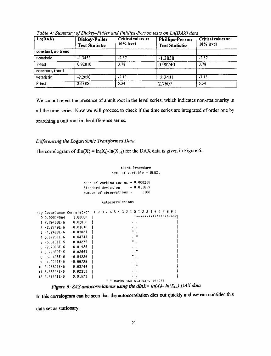
Table 4: Summary o f Dickey-Fuller and Phillips-Perron tests on Ln(DAX) dataLn(DAX) Dickey-Fuller

Test StatisticCritical values at 10% level

Phillips-Perron Test Statistic

Critical values at 10% level

constant, no trend

t-statistic -1 .3 4 5 3 -2 .57 -1.3858 -2 .57

F-test 0 .9 2 8 1 0 3.78 0.98240 3.78

constant, trend

t-statistic -2 .2 0 5 0 -3.13 -2.2431 -3 .13

F-test 2 .6885 5.34 2.7607 5.34

We cannot reject the presence of a unit root in the level series, which indicates non-stationarity in

all the time series. Now we will proceed to dheck if the time series are integrated of order one by

searching a unit root in the difference series.

Differencing the Logarithmic Transformed Data

The correlogram of dln(X) = ln(Xt)-ln(Xt_i) for the DAX data is given in Figure 6.

ARIMA Procedure

Name of va ria b le = DLNX.

Mean of working se ries = 0.000268

Standard dev ia tion = 0.011859

Number of observations = 1188

A u to co rre la t i ons

Lag Covariance C o rre la tio n - 1 9 8 7 6 5 4 3 2 1 0 1 2 3 4 5 6 7 8 9 1

0 0.00014064 1.00000 1 J 1

1 2.89408E-6 0.02058 1

2 -2.2749E-6 -0.01618 1

3 -4.2489E-6 -0.03021 1 * 1. 1

4 6.67231E-6 0.04744 1 . 1* 1

5 -6.0131E-6 -0.04275 1 ★ ( . 1

6 -2.7093E-6 -0.01926 1

7 3.72859E-6 0.02651 1 • 1* 1

8 -5.9435E-6 -0.04226 1★ 1 1

9 -1.0241E-6 -0.00728 1 • 1 · 1

10 5.26501E-6 0.03744 1 • 1* 1

11 3.25242E-6 0.02313 1

12 2.21241E-6 0.01573 1marks two standard e rro rs

Figure 6: SAS autocorrelations using the dlnX= ln(X,)- ln(X,.i) DAX data

In this correlogram can be seen that the autocorrelation dies out quickly and we can consider this

data set as stationary.

21

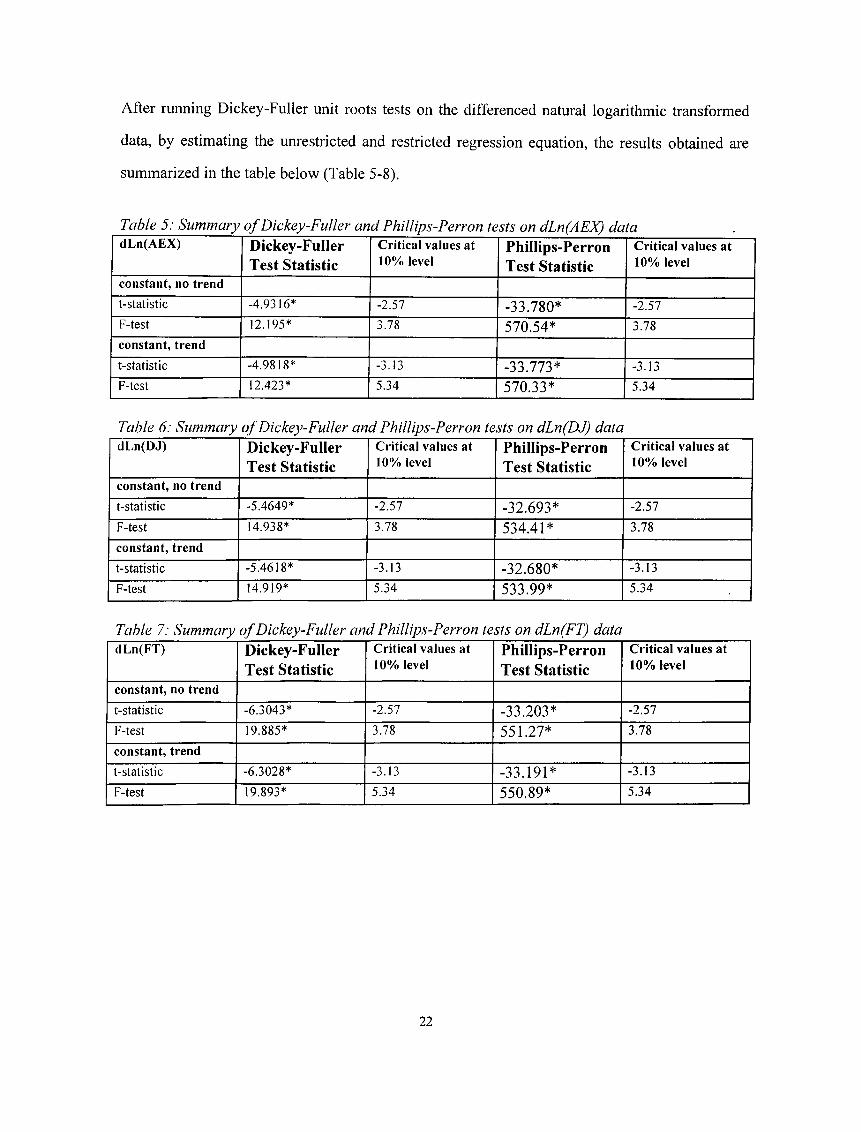
After running Dickey-Fuller unit roots tests on the differenced natural logarithmic transformed

data, by estimating the unrestricted and restricted regression equation, the results obtained are

summarized in the table below (Table 5-8).

Table 5: Summary o f Dickey-Fuller and Phillips-Perron tests on dLn(AEX) datad L n (A E X ) Dickey-Fuller

Test StatisticC ritica l va lues at 10% level

Phillips-Perron Test Statistie



t-statistic -4 .9316* -2.57 - 3 3 .7 8 0 * -2 .57

F-test 12.195* 3.78 5 7 0 .5 4 * 3.78

con stan t, trend

t-statistic -4 .9818* -3.13 - 3 3 .7 7 3 * -3.13

F-test 12.423* 5.34 5 7 0 .3 3 * 5.34

Table 6: Summary o f Dickey-Fuller and Phillips-Perron tests on dLn(DJ) datad l.n (D J ) Dickey-Fuller

Test StatisticC ritica l va lu es at 10% level




t-statistic -5 .4649* -2.57 - 3 2 .6 9 3 * -2 .57

F-test 14.938* 3.78 5 3 4 .4 1 * 3 .78

con stan t, trend

t-statistic -5 .4618* -3.13 - 3 2 .6 8 0 * -3 .13

F-test 14.919* 5.34 5 3 3 .9 9 * 5.34

Table 7: Summary o f Dickey-Fuller and Phillips-Perron tests on dLn(FT) datatlL n (F T ) Dickey-Fuller





t-statistic -6 .3043* -2.57 - 3 3 .2 0 3 * -2 .57

F-test 19.885* 3.78 5 5 1 .2 7 * 3 .78

con stan t, trend

t-statistic -6 .3028* -3.13 - 3 3 .1 9 1 * -3.13

F-test 19.893* 5.34 5 5 0 .8 9 * 5 .34

22

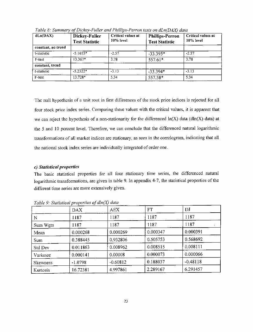
Table 8: Summary o f Dickey-Fuller and Phillips-Perron tests on dLn(DAX) datad L n (D A X ) Dickey-Fuller




co n sta n t, no trend

t - s t a t i s t i c -5 .1655* -2 .57 -33.395* -2 .57

F - te s t 13.367* 3.78 557.61* 3.78

con stan t, trend

t - s t a t i s t i c -5 .2322* 3.13 -33.394* -3 .13

F - te s t 13.728* 5.34 557.58* 5.34

The null hypothesis of a unit root in first dilTerences of the stock price indices is rejected for all

four stock price index series. Comparing these values with the critical values, it is apparent that

we can reject the hypothesis of a non-stationarity for the differenced ln(X) data (dln(X) data) at

the 5 and 10 percent level. Therefore, we can conclude that the differenced natural logarithmic

transformations of all market indices are stationary, as seen in the correlogram, indicating that all

the national stock index series are individually integrated of order one.

c) Statistical propertiesThe basic statistical properties for all four stationary time series, the differenced natural logarithmic transformations, are given in table 9. In appendix 4-7, the statistical properties of the different time series are more extensively given.

Table 9: Statistical properties ofdln(X) dataDAX AEX FT DJ

N 1187 1187 1187 1187

Sum Wgts 1187 1187 1187 1187

Mean 0.000268 0.000269 0.000347 0.000391

Sum 0.388445 0.932806 0.505753 0.568692

Std Dev 0.011863 0.008962 0.008515 0.008111

Variance 0.000141 0.00008 0.000073 0.000066

Skewness -1.0798 -0.60812 0.188037 -0.48118

Kurtosis 16.72381 4.997861 2.289167 6.291457

23

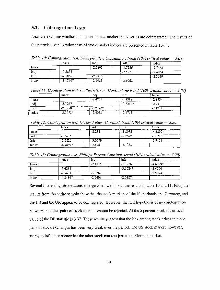
5.2. Cointegration Tests

Next we examine whether the national stock market index series are cointegrated. The results of

the pairwise cointegration tests of stock market indices are presented in table 10-11.

Table 10: Cointegration test, Dickey-Fuller: Constant, no trend (10% critical value = -3.04)Inaex Indj Inft Indax

Inaex -2 .2893 -1 .7536 -2 .7463Indj -2 .5833 -2 .5973 -2 .4034Inft -2 .1856 -2 .8910 -2 .3049Indax -3 .1790* -2 .6983 -2 .1962

Table 11: Cointegration test, Phillips-Perron: Constant, no trend (10%> critical value = -3.04)Inaex Indj Inft Indax

Inaex -2.4751 -1 .8388 -2 .8534Indj -2 .7767 -3 .2214* -2 .4313Inft -2 .1 9 5 0 -3 .2290* -2 .1718Indax -3 .1473* -2 .4033 -2 .1765

Table 12: Cointegration test, Dickey-Fuller: Constant, trend (10% critical value = -3.50)Inaex Indj Inft Indax

Inaex -2.2841 -1 .8085 -4 .3802*

Indj -2 .5615 -2 .7627 -3 .0213

Inft -2 .2826 -3 .0279 -2 .9154

Indax -4 .4694* -2.4461 -2 .1063

Table 13: Cointegration test, Phillips-Perron: Constant, trend (10% critical value = -3.50)Inaex Indj Inft Indax

Inaex -2 .4835 -1 .7976 -4 .6999*

Indj -3.6281 -3 .6024* -3 .4560

Inft -2.5431 -3 .0287 -2 .5094Indax -4 .8486* -2 .5409 -2 .0887

Several interesting observations emerge when we look at the results in table 10 and 11. First, the

results from the entire sample show that the stock markets of the Netherlands and Germany, and

the US and the UK appear to be cointegrated. However, the null hypothesis of no cointegration

between the other pairs of stock markets cannot be rejected. At the 5 percent level, the critical

value of the DF statistic is 3.37. These results suggest that the link among stock prices in those

pairs of stock exchanges has been very weak over the period. The US stock market, however,

seems to influence somewhat the other stock markets just as the German market.

24

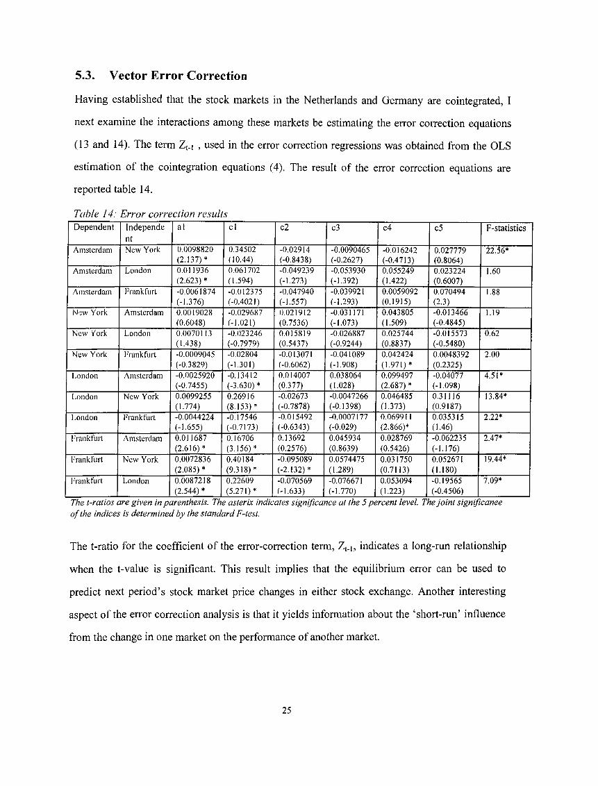
5.3. Vector Error Correction

Having established that the stock markets in the Netherlands and Germany are cointegrated, I

next examine the interactions among these markets be estimating the error correction equations

(13 and 14). The term Zt.i , used in the error correction regressions was obtained from the OLS

estimation of the cointegration equations (4). The result of the error correction equations are

reported table 14.

Table 14: Error correction resultsD e p e n d e n t I n d e p e n d e

n t

a l c 2 c3 c 4 c 5 F - s ta t i s t i c s

Amsterdam New York 0.0098820

(2.137)*

0.34502

(10.44)

-0.02914

(-0.8438)

-0.0090465

(-0.2627)

-0.016242

(-0.4713)

0.027779

(0.8064)

22.56*

Amsterdam London 0.011936

(2.623)*

0.061702

(1.594)

-0.049239

(-1.273)

-0.053930

(-1.392)

0.055249

(1.422)

0.023224

(0.6007)

1.60

Amsterdam Frankfurt -0.0061874

(-1.376)

-0.012375

(-0.4021)

-0.047940

(-1.557)

-0.039921

(-1.293)

0.0059092

(0.1915)

0.070494

(2.3)

1.88

New York Amsterdam 0.0019028

(0.6048)

-0.029687

( - 1.021)0.021912

(0.7536)

-0.031171

(-1.073)

0.043805

(1.509)

-0.013466

(-0.4845)

1.19

New Vork London 0.0070113

(1.438)

-0.023246

(-0.7979)

0.015819

(0.5437)

-0.026887

(-0.9244)

0.025744

(0.8837)

-0.015573

(-0.5480)

0.62

New York Frankfurt -0.0009045

(-0.3829)

-0.02804

(-1.301)

-0.013071

(-0.6062)

-0.041089

(-1.908)

0.042424

(1.971)*

0.0048392

(0.2325)

2.00

London Amsterdam -0.0025920

(-0.7455)

-0.13412

(-3.630) *

0.014007

(0.377)

0.038064

(1.028)

0.099497

(2.687) *

-0.04077

(-1.098)

4.5 D

London New York 0.0099255

(1.774)

0.26916

(8.153)*

-0.02673

(-0.7878)

-0.0047266

(-0.1398)

0.046485

(1.373)

0.31116

(0.9187)

13.84*

London Frankfurt -0.0044224

(-1.655)

-0.17546

(-0.7173)

-0.015492

(-0.6343)

-0.0007177

(-0.029)

0.069911

(2 .866)*

0.035315

(1.46)

2.22*

’̂rankfurt Amsterdam 0.011687

(2.616)*

0.16706

(3.156)*

0.13692

(0.2576)

0.045934

(0.8639)

0.028769

(0.5426)

-0.062235

(-1.176)

2.47*

Frankfurt New York 0.0072836

(2.085) *

0.40184

(9.318)*

-0.095089

(-2.132)*

0.0574475

(1.289)

0.031750

(0.7113)

0.052671

(1.180)

19.44*

f'rankfurt London 0.0087218

(2.544) *

0.22609

(5.271)*

-0.070569

M.633)

-0.076671

(-1.770)

0.053094

(1.223)

-0.19565

(-0.4506)

7.09*

The (-ratios are given in parenthesis. The asterix indicates significance at the 5 percent level The joint significance o f the indices is determined by the standard F-tesl.

The t-ratio for the coefficient of the error-correction term, Zn, indicates a long-run relationship

when the t-value is significant. This result implies that the equilibrium error can be used to

predict next period’s stock market price changes in either stock exchange. Another interesting

aspect of the error correction analysis is that it yields information about the ‘short-run’ influence

from the change in one market on the performance of another market.

25

The results (table 14) of the application of the VEC model on the different time series indicate a

substantial short-term and long-term relationship between the German and British market, as well

as between the British and Dutch market. Although the short-run influences from changes in one

market on the other market are not as substantial as in the case of the US on the three European

markets, they are significant. In the case of these two pairs of national markets, the earlier

reported test have not indicated significant cointegration.

In contrast, table 10-13 show that the stock markets of the Netherlands and Germany appear to be

cointegrated. However, table 14 reports that Amsterdam has a significant impact on the German

stock market in the long-run, but not vice versa. Furthermore, short-run changes in the Dutch

stock market seem to have a significant influence on the German market.

The results in table 14 report a significant impact of the US on the three European markets in the

short- and long-run for the period examined. In all regressions reported in table 14, the results

show that the US market exerts especially a substantial amount of influence in the short-run with

F-values of 22.56, 13.84 and 19.44 on Amsterdam, London, and Frankfurt, respectively.

Flowever, other tests have reported no significant cointegration between the US and the European

markets. In contrast, European ‘short- and long-run’ stock market changes do not appear to have

any significant impact on the US stock market. This result is inconsistent with the view that

foreign stock market innovations have exerted substantial influence on the US market in the post-

October 1987 period.

26

6. Conclusion

The theory of causality and the notion of cointegration is used to examine linkages and dynamic

interactions among stock price indices in four stock exchanges (Amsterdam, London, New York

and Frankfurt) by means of the error-correction model. The data used in this study are daily

closing prices of the stock exchanges. The sample consists of 1188 observations and covers the

period of March 1990 through October 1994.

Tests of stationarity allow us to conclude that the level series are nonstationary, but the

difference series are stationary. Thus, prices are integrated of order one, 1(1), and the use of the

vector error correction model is appropriate to test for long- and short-run interdependencies

between the four stock exchanges. The error-correction analysis produced some interesting

results with respect to the stock market interactions among the four stock exchanges.

The US market exerts a significant long-term impact on the European markets, but not vice

versa. Moreover, the US stock price index variable has a substantial amount of short-term

influence on all other markets. This result is inconsistent with the view that foreign stock market

innovations have exerted substantial influence on the US market in the post-October 1987 period.

The three European markets also influence each other in the short- and long-run, with the

exception of Amsterdam that not seems to be influenced significantly by the German market.

This result implies that these markets are not independent from each other but move together.

This can be explained by the fact that the three countries are members of the European Union.

The implementation of some institutional agreements of the European Union concerning equity

markets, the exchange rate mechanism that is partly coordinated among the countries, and

intensive trade and other cooperation between the national governments have removed many

barriers and resulted in a high degree of integration. As a result, the markets have been

27

globalized. Previous studies have made a strong case for international portfolio diversification to

reduce the risk of a portfolio while enhancing the performance opportunities. However, the

condition that national stock markets lack interdependence is rejected for the examined stock

exchanges because of significant reported short- and long-term linkages. Therefore,

diversification among those national stock markets will not greatly reduce the portfolio risk

without sacrificing expected return.

28

References:

Aggerwal, R., and Y.S. Park, 1994, The relationship between daily US and Japanese equity prices: Evidence from spot versus futures markets. Journal of Banking and Finance 18, 757-773

Agmon, T., 1972, The relations between equity markets: A study o f share price co-movements in the United States, United Kingdom, Germany, Japan, Journal of Finance 27, 839-855

Ambler, S., 1989, Does money matter in Canada? Evidence from a vector error correction model, Jlie Review of Economics and Statistics, 651-658

Ammer, J., J. Mei, 1994, Measuring international economic linkages with stock market data. The Journal of Finance 1994, 1044-1045

Arshanapalli, B., J. Doukas, 1993, International stock market linkages: Evidence from the pre- andpost-October 1987period. Journal of Banking and Finance 17, 193-208

Becker, K.G., J.E. Finnerty and M. Gupta, 1990, The intertemporal relation between the US and Japanese stock markets. Journal of Finance 45, 1297-1306

Bertera, E., C. Mayer, 1990, Structure and performance: Global interdependence o f stock markets around the crash o f1987, Euopean Economic Review 34, 1155-1180

Chan, K.C., B.E. Gup and M.S. Pan, 1992, An emperical analysis o f stock prices in major Asian markets and the United States, The Financial Review 27, 289-307

Chowdhury, A.R., 1994, Stock market interdependencies: Evidence from the Asian NIEs, Journal of Macroeconomics 16, 629-651

Dwyer, G.P., and R.W. Hafer, 1988, Are national stock markets linked?. Federal Reserve Bank of St. Louis Review 70, 3-14

Engle, R.F., C.W. Granger, 1987, Co-integration an error correcion: representation, estimation, and testing, Econometrica 55, 251-276

29

Engle, R.F., B.S. Yoo, 1987, Forecasting and testing in co-integrated systems, Journal of Econometrics 35, 143-159

Eun, C.S., S. Shim, 1989, International transmission o f stock market movements. Journal of Financial and Quantitative Analysis 24, 241-256

Gultekin, M., B. Gultekin and A. Penati, 1989, Capital controls and international capital markets: The evidence from the Japanese and American stock markets. Journal of Finance 44, 849-869

Flamao, Y., R.W. Masulis, and V. Ng, 1990, Correlations in price changes and volatility across international stock markets. The Review of Financial Studies Vol 3, No.2, 281-307

Hylleberg, S., R.F. Engle, and C.W.J. Granger, 1990, Seasonal integration and cointegration. Journal of Econometrics 44, 215-238

Jorion, P., E. Schwartz, 1986, Integration versus segmentation in the Canadian stock market. Journal of Finance 41, 603-616

Kasa, K., 1992, Common stochastic trends in international stock markets. Journal of Monetary Economics 29, 95-124

Koutoulas, G., and L. Kryzanowski, 1994, Integration or segmentation o f the Canadian stock market: evidence based on the APT, Canadian Journal of Economics 2, 329-351

Kwan, A.C.C., A.B. Sim, and J.A. Cotsomitis, 1995, The causal relationships between equity indices on world exchanges. Applied Economics 27, 33-37

Lee, I., R. Petitt, and M.V. Swankoski, 1990, Daily return relationships among asian stock markets. Journal of Business Finance and Accounting 17,265-284

Lessard, D.A., 1976, International diversification. Financial Analyst Journal 32, Feb. 32-38

Malliaris, A.G., and J. Urrita, 1992, The international crash o f October 1987: causality tests. Journal of Finance and Quantitative Analysis 27, 353-364

30

Mathur, I., V. Subrahmanyam, 1990, Interdependencies among the nordic and US stock markets, Scandinavian Journal of Economics 4, 587-597

Meric, 1., G. Meric, 1989, Potential gains from international portfolio diversification and intertemporal stability and seasonality in international stock market relationships. Journal of Banking and Finance 13, 627-640

Rogers, J.H., 1994, Entry barriers and price movements between major and emerging stock markets. Journal of Macroeconomics 16, 221-241

Smith, K.L., J. Brocato, and J.E. Rogers, 1993, Regularities in the data between major equity markets: evidence from Granger causality tests. Applied Financial Economics 3, 55-60

Von Furstenberg, G.M., B.N. Jeon, 1990, Growing international comovements in stock price indexes. Quarterly Review of Economics and Business 30,15-30

31

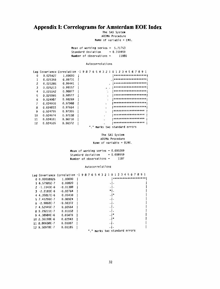
Appendix I: Correlograms for Amsterdam EOE IndexThe SAS System

ARIMA Procedure

Name of va ria b le = LNX.

Mean of working se rie s = 5.71753

Standard d ev ia tio n = 0.159459


A u to co rre la t i ons

Lag Covariance C o rre la tio n -1 9 8 7 6 5 4 3 2 1 0 1 2 3 4 5 6 7 8 9 1

0 0.025427 1.00000 11 *★ ★ **★ *·*·★ ★ ★ ★ ★ ★ ★ ★ ★ ★ ★ ★

1 0.025359 0.99731 11

2 0.025285 0.99441 11

3 0.025213 0.99157 1J

4 0.025142 0.98877 11 ★ ★ ■*·★ *★ *★ ★ *****★ ★ ★ ★ ★ ★

5 0.025065 0.98577 11

6 0.024987 0.98269 1I*★ ★ ★ ★ *★ ★ *★ *★ *★ **★ ★ ★ *

7 0.024910 0.97968 1j **★ ★ ★ ★ ★ ★ ★ *★ ****★ ★ ★ ■*·* 1

8 0.024833 0.97664 1I j

9 0.024755 0.97355 11 *■*·★ ★ ★ ★ *★ **★ *★ ★ ·*·*··*·★ ★ j

10 0.024674 0.97038 11 ★ ****★ ★ ★ *-**★ ★ ★ *★ ★ ★ * 1

11 0.024591 0.96710 11★ ★ **★ **★ **★ *★ ★ *★ *★ * 1

12 0.024505 0.96372 11 1

marks two standard e rro rs

The SAS System

ARIMA Procedure



Standard dev ia tio n = 0.008959


Au toco rre la tio ns


0 0.00008026 1.00000 1 j j

1 6.57985E-7 0.00820 1

2 -1.1143E-6 -0.01388 1

3 -2.2183E-6 -0.02764 1 *1. 1

4 4.35817E-6 0.05430 1 1 1

5 7.41296E-7 0.00924 1 • 1 * 1

6 -2.9868E-7 -0.00372 1 • 1 · 1

7 4.52945E-7 0.00564 1

8 9.29215E-7 0.01158 1

9 4.38984E-6 0.05470 1 . 1 * 1

10 2.36198E-6 0.02943 1 1 * 1

11 8.80638E-7 0.01097 1 • 1 * 1

12 9.50978E-7 0.01185 1marks two s ta n d ard e r r o r s

32

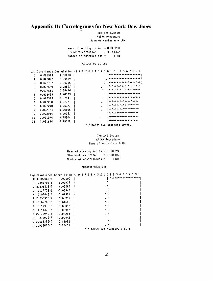
Appendix II: Correlograms for New York Dow JonesThe SAS System

ARIMA Procedure





Au toco rre la tions

Lag Covariance C o rre la tio n - 1 9 8 7 6 i 5 4 3 2 1 0 1 2 3 4 5 6 7 8 9 1

0 0.022914 1.00000 1 1 *********************

1 0.022822 0.99599 1 I ★★★★★★★★★★★■A··*·***·*·***

2 0.022732 0.99206 1 j *■*■·*·★★·*·★★★★★★★**■*·*★★★

3 0.022640 0.98807 1 1*★*★★*★★**★*★**★**★*

4 0.022551 0.98416 1 1★★★★★★★★★★★★★★★★★★★★

5 0.022463 0.98033 1 1

6 0.022373 0.97641 1 1 ★■*·★★·*■·*■★■*★·*★·*■★·*·★■*·■*·■*■★★

7 0.022288 0.97271 11 *★★**★★★****★*·*·★*★*

8 0.022210 0.96927 11★★★★★★★★★★★★★★★★★★*

9 0.022134 0.96596 11★★★★**★★★★★★★★★★★★★

10 0.022055 0.96253 11★★★★★★★★*★***★★★★★★

11 0.021975 0.95904 11★*★★*★★*★*★★**★**★*

12 0.021894 0.95552 11★****★★★*★★★★★★★*★★


The SAS System

ARIMA Procedure


Mean of working series = 0.000391


Number of observations 1187

Autoco rre la tions

-ag Covariance C o rre la tio n - 1 9 8 7 6 5 4 3 2 1 0 1 2 3 4 5 6 7 8 9 1

0 0.00006575 1.00000 1 I 1

1 1.26179E-6 0.01919 1

2 8.53557E-7 0.01298 1 • 1 · 1

3 -1.2777E-6 -0.01943 1

4 -1.9704E-6 -0.02997 1 ★ 1. 1

5 2.55598E-7 0.00389 1 • 1 · 1

6 -3.0276E-6 -0.04605 1 ★ 1 1

7 -3.9793E-6 -0.06052 1 ★ 1. 1

8 -1.9442E-6 -0.02957 1 ★ 1. 1

9 2.13894E-6 0.03253 1 • 1* I

10 -2.909E-7 -0.00442 1

11 2.59835E-6 0.03952 1 . 1* 1

12 2.93585E-6 0.04465 1 . 1* 1

marks two s ta n d a rd e r r o r s

33

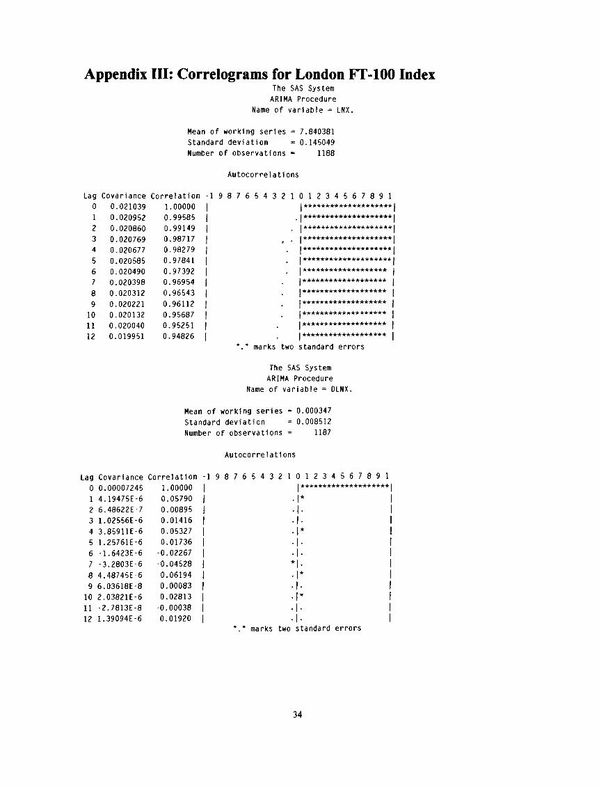
Appendix III: Correlograms for London FT-100 IndexThe SAS System

ARIMA Procedure



Standard d ev ia tio n = 0.145049


A u toco rre la tions

Lag Covariance C o rre la tio n -1 9 8 7 6 5 4 3 2 1 0 1 2 3 4 5 6 7 8 9 1

0 0.021039 1.00000 1I

1 0.020952 0.99585 1^1*★★★★★★+****★***★★**

2 0.020860 0.99149 11 ★★★★★★★★★★★★★★★★★★★■A'

3 0.020769 0.98717 1 *1

4 0.020677 0.98279 11

5 0.020585 0.97841 1 . I * * * * * * * * * * * * * * * * * * * *

6 0.020490 0.97392 1 . 1 * * * * * * * * * * * * * * * * * * *

7 0.020398 0.96954 1 . 1 * * * * * * * * * * * * * * * * * * * j

8 0.020312 0.96543 1 . I * * * * * * * * * * * * * * * * * * * j

9 0.020221 0.96112 1 . j *★★*★★★*★■*··*·*·*★*■*·★** j

10 0.020132 0.95687 11 1

11 0.020040 0.95251 1 . 1***★*★*★★★★★**★★★★★ 1

12 0.019951 0.94826 1 . 1 * * * * * * * * * * * * * * * * * * * 1


The SAS System

ARIMA Procedure



Standard dev ia tio n = 0.008512


Au toco rre la tions


0 0.00007245 1.00000 1 j *·*■★★*★★★*★★★★★**★★** 1

1 4.19475E-6 0.05790 1 . 1 * 1

2 6.48622E-7 0.00895 1

3 1.02556E-6 0.01416 1 . 1. 1

4 3.85911E-6 0.05327 1 . 1 * 1

5 1.25761E-6 0.01736 1 * 1 * 1

6 -1.6423E-6 -0.02267 1

7 -3.2803E-6 -0.04528 1 ^|. 1

8 4.48745E-6 0.06194 1 i * 1

9 6.03618E-8 0.00083 1

10 2.03821E-6 0.02813 1 j * j

11 -2.7813E-8 -0.00038 1

12 1.39094E-6 0.01920 1 * 1 * 1marks two s tan d ard e r r o r s

34

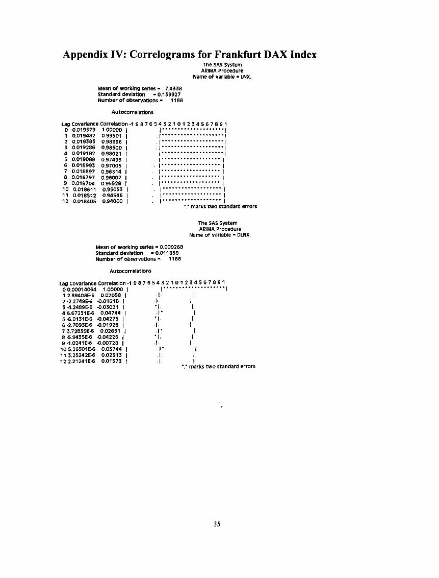
Appendix IV: Correlograms for Frankfurt DAX Index

Mean of working series - 7.4538 Standard deviation - 0.139927 Number of observations - 1188

The SAS System ARiMA Procedure

Name of variabie - LNX.

Autocorreiations

Lag Covariance Correiation -1 9 8 7 6 5 4 3 2 1 0 1 2 3 4 5 6 7 8 9 10 0.019579 1.00000 i 1............ * .......................... M1 0.019482 0.99501 i2 0.019383 0.98996 i3 0.019286 0.98500 i4 0.019192 0.98021 15 0.019089 0.97495 16 0.018993 0.97005 17 0.018897 0.96514 i8 0.018797 0.96002 i 1

9 0.018704 0.95528 i10 0.018611 0.95053 1 I - - - - - * * * * - * * * 111 0.018512 0.94546 I12 0.018405 0.94000 i . i ......................................... 1

' marks two standard errors

The SAS System ARiMA Procedure

Name of variabie - DLNX.

Mean of working series - 0.000268 Standard deviation - 0.011859 Number of observations - 1188

Autocorreiations

Lag Covariance Correiation -1 9 8 7 6 5 4 3 2 1 0 1 2 3 4 5 6 7 8 9 10 0.000140641 2.89408E-62 -2.2749E-63 ^.2489E-64 6.67231 E-6 5-6.0131E-66 -2.7093E-67 3.72859E-68 -5.9435E-6 9-1.0241 E-6

10 5.26501 E-611 3.25242E-612 2.21241 E-6

1.00000 i 0.02058 i

-0.01618 i -0.03021 i

0.04744 i -0.04275 i -0.01926 i

0.02651 I -0.04226 i -0.00728 I

0.03744 I 0.02313 I 0.01573 i

r

I

I' marks two standard errors

35

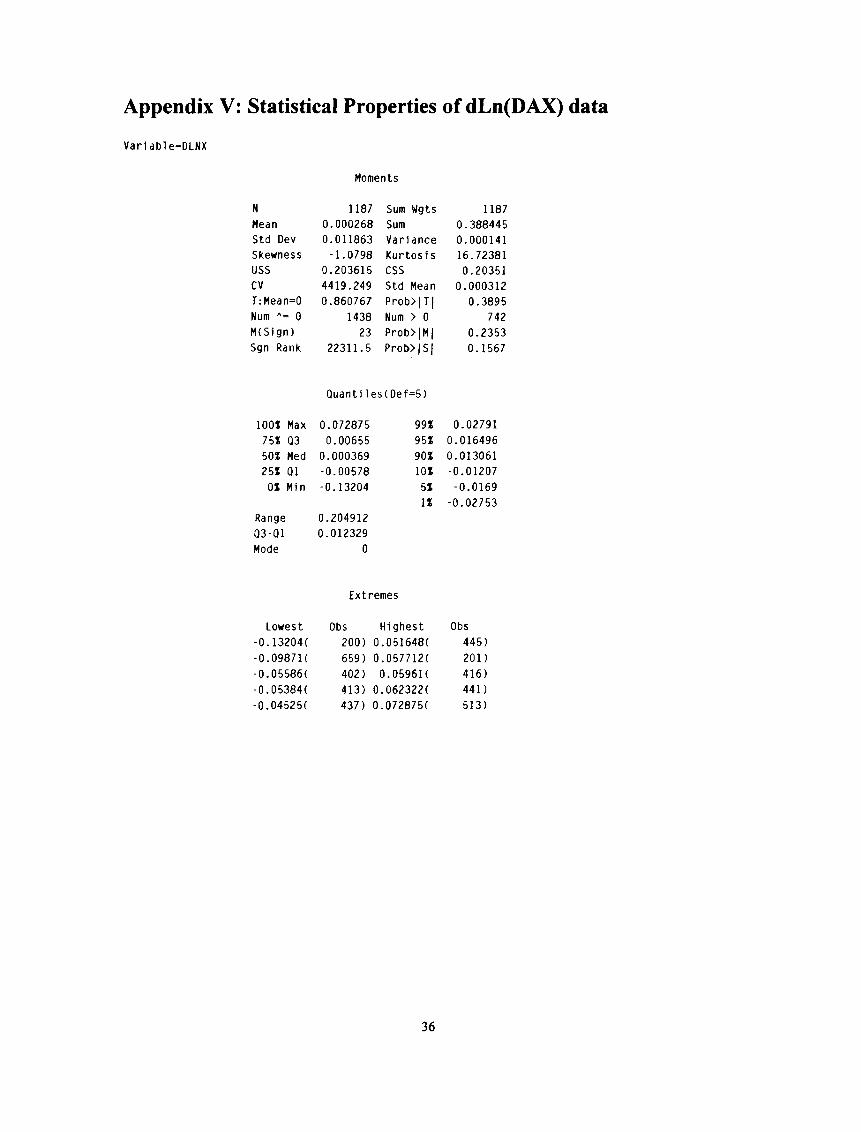
Appendix V: Statistical Properties o f dLn(DAX) data

Variable=DLNX

Moments

N 1187 Sum Wgts 1187

Mean 0.000268 Sum 0.388445

Std Dev 0.011863 Variance 0.000141

Skewness -1.0798 Kurtos is 16.72381

USS 0.203615 CSS 0.20351

CV 4419.249 Std Mean 0.000312

T:Mean=0 0.860767 Prob>|T| 0.3895

Num 0 1438 Num > 0 742

M(Sign) 23 Prob>|M| 0.2353

Sgn Rank 22311.5 Prob>|S| 0.1567

Quantiles(Def=5)

100% Max 0.072875 99% 0.02791

75% Q3 0.00655 95% 0.016496

50% Med 0.000369 90% 0.013061

25% Q1 -0.00578 10% -0.01207

0% Min -0.13204 5% -0.0169

1% -0.02753

Range 0.204912

Q3-Q1 0.012329

Mode 0

Extremes

Lowest Obs Highest Obs

-0.13204C 200) 0 .051648( 445)

-0.0987K 659) 0 .057712( 201)

-0.05586( 402) 0.0596K 416)

-0.05384( 413) 0 .062322( 441)

-0.04525( 437) 0.072875( 513)

36

Appendix VI: Statistical Properties o f dLn(AEX) data

Variable=DLNX

Moments


Mean 0.000269 Sum 0.392806


Skewness -0.60812 Kurtos is 4.997861

USS 0.117201 CSS 0.117096

CV 3328.654 Std Mean 0.000235

T:Mean=0 1.147516 Prob>|T| 0.2514

Num '"= 0 1455 Num > 0 774M(Sign) 46.5 Prob>|M| 0.0158

Sgn Rank 40421.5 Proly>|S| 0.0116

Q uanti)es(Def=5)

100% Max 0.051059 99% 0.021694

75% 03 0.005391 95% 0.013341

50% Med 0.000583 90% 0.01011

25% 01 -0.00446 10% -0.00967

0% Min -0.06794 5% -0.01376

1% -0.02636

Range 0.118997

03-01 0.009853

Mode 0

Extremes

Lowest Obs Hi ghest Obs

-0.06794( 202) 0.028566( 429)

-0.05033( 665) 0.030616C 449)

-0.04109( 404) 0.035642( 936)

-0.03627( 951) 0.040124( 419)

-0.03597( 84) 0.051059C 518)

37

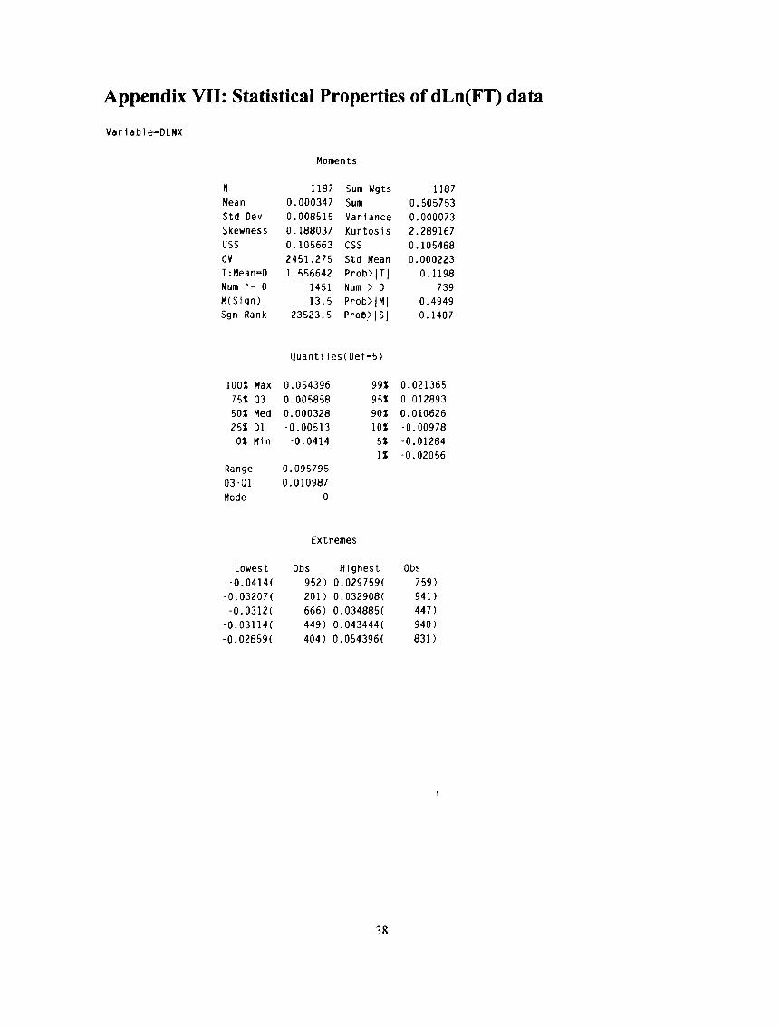
A ppendix VII: Statistical Properties o f dLn(FT) data

Var1able=DLNX

Moments

N

Mean

1187

0.000347

Sum Wgts

Sum

1187

0.505753

Std Dev 0.008515 Vari ance 0.000073

Skewness 0.188037 Kurtos is 2.289167

USS 0.105663 CSS 0.105488

CV 2451.275 Std Mean 0.000223

T:Mean=0 1.556642 Prob>|T| 0.1198

Num ''= 0 1451 Num > 0 739

M(Sign) 13.5 Prob>|M| 0.4949

Sgn Rank 23523.5 Prob>|S| 0.1407

Q uan ti1es(Def=5)

lOOX Max 0.054396 99% 0.021365

75% Q3 0.005858 95% 0.012893

50% Med 0.000328 90% 0.010626

25% Q1 -0.00513 10% -0.00978

0% Min -0.0414 5% -0.01284

1% -0.02056

Range 0.095795

Q3-Q1 0.010987

Mode 0

Extremes

Lowest Obs Hi ghest Obs

-0.0414( 952) 0 .029759( 759)

-0.03207( 201) 0 .032908( 941)

-0.0312( 666) 0 .034885( 447)

-0.03114( 449) 0 .043444( 940)

-0.02859( 404) 0 .054396( 831)

38

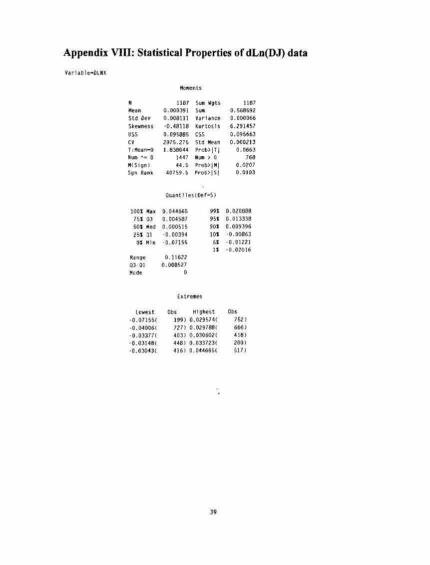
Appendix VIII: Statistical Properties o f dLn(DJ) data

Variable=DLNX

Moments


Mean 0.000391 Sum 0.568692


Skewness -0.48118 Kurtosis 6.291457

USS 0.095885 CSS 0.095663

CV 2075.275 Std Mean 0.000213

T:Mean=0 1.838044 Prob>|T| 0.0663

Num 0 1447 Num > 0 768

M(Si gn) 44.5 Prob>|M| 0.0207

Sgn Rank 40759.5 Prob>|S| 0.0103

Quantiles (Def=5)

100% Max 0.044665 99% 0.020888

75% Q3 0.004587 95% 0.013338

50% Med 0.000515 90% 0.009396

25% Q1 -0.00394 10% -0.00863

0% Min -0.07155 5% -0.01221

1% -0.02016

Range 0.11622

Q3-Q1 0.008527

Mode 0

Extremes

Lowest Obs 1̂ ighest Obs

-0.07155( 199) 0 .029574( 752)

-0.04006( 727) 0 .029788( 666)

-0.03377( 403) 0 .030602( 418)

-0.03148( 448) 0,.033723( 200)

-0.03043( 416) 0,.044665( 517)

39

>»ί· ili:, ϊ., 1·«γ4 - thesis.bilkent.edu.tr

Documents

Transcript of >»ί· ili:, ϊ., 1·«γ4 - thesis.bilkent.edu.tr