Global minimization using an Augmented Lagrangian method

with variable lower-level constraints

E. G. Birgin ∗ C. A. Floudas † J. M. Martınez ‡

November 22, 2006

Abstract

A novel global optimization method based on an Augmented Lagrangian framework isintroduced for continuous constrained nonlinear optimization problems. At each outer it-eration the method requires the ε-global minimization of the Augmented Lagrangian withsimple constraints. Global convergence to an ε-global minimizer of the original problem isproved. The subproblems are solved using the αBB method. Numerical experiments arepresented.

Key words: deterministic global optimization, Augmented Lagrangians, nonlinear pro-gramming, algorithms, numerical experiments.

1 Introduction

Global optimization has ubiquitous applications in all branches of engineering sciences andapplied sciences. During the last decade several textbooks addressed different facets of globaloptimization theory and applications [17, 28, 33, 44, 77, 86, 87, 91]. Recent review papers havealso appeared [29, 68].

The Augmented Lagrangian methodology based on the Powell-Hestenes-Rockafellar [43, 70,72] formula has been successfully used for defining practical nonlinear programming algorithms[12, 13, 19, 23]. Convergence to KKT points was proved using the Constant Positive LinearDependence constraint qualification [11], which strengthens the results based on the classicalregularity condition [18, 23].

∗Department of Computer Science IME-USP, University of Sao Paulo, Rua do Matao 1010, Cidade Univer-sitaria, 05508-090, Sao Paulo SP, Brazil. This author was supported by PRONEX-Optimization (PRONEX- CNPq / FAPERJ E-26 / 171.164/2003 - APQ1), FAPESP (Grants 06/53768-0 and 06/51827-9) and CNPq(PROSUL 490333/2004-4). e-mail: egbirgin@ime.usp.br

†Department of Chemical Engineering, Princeton University, Princeton, NJ 08544, USA. This author wassupported by the National Science Foundation and the National Institute of Health (R01 GM52032). e-mail:floudas@titan.princeton.edu

‡Department of Applied Mathematics, IMECC-UNICAMP, University of Campinas, CP 6065, 13081-970Campinas SP, Brazil. This author was supported by PRONEX-Optimization (PRONEX - CNPq / FAPERJE-26 / 171.164/2003 - APQ1), FAPESP (Grant 06/53768-0) and CNPq. e-mail: martinez@ime.unicamp.br

1

In this work, we consider the Augmented Lagrangian method introduced in [13] and we mod-ify it in such a way that, at each outer iteration, we find an ε-global minimizer of the subproblem.In the definition of the subproblem we introduce an important modification with respect to [13]:besides the lower level constraints we include constraints that incorporate information about theglobal solution of the nonlinear programming problem. A theorem of convergence to ε-globalminimizers is presented.

We consider linear constraints on the lower-level set, and additional valid linear constraintswhich result from outer approximations of the feasible region and hence incorporate the globaloptimum information. This allows us to use the αBB [3, 4, 5, 15, 28, 50, 51, 57, 58, 59] methodand its convex underestimation techniques [5, 6, 8, 9, 21, 42, 60, 63, 64, 66] for the subproblemsin such a way that the underestimation techniques are applied just to the Augmented Lagrangianfunction and not to the constraints. The αBB global optimization approach has been applied tovarious problems that include molecular conformations in protein folding [16, 46, 47, 48, 49, 89],parameter estimation [24, 25, 26, 27], and phase equilibrium [39, 40, 41, 61, 62]. Mixed-integernonlinear models arising in process synthesis, design and operations problems [1, 2, 7, 22, 30,31, 52] represent additional important application areas.

It is important to emphasize that many global optimization techniques for nonlinear program-ming problems, e.g., [4, 5, 10, 15, 32, 34, 35, 36, 37, 38, 53, 54, 69, 74, 75, 78, 79, 80, 81, 82, 83, 88].However, to our knowledge, none of them is based on Augmented Lagrangians. Moreover, as aconsequence of using the Augmented Lagrangian approach combined with the αBB method andits convex α-underestimation techniques, the method introduced in this paper does not rely onthe functional form of the functions involved in the problem definition (objective function andconstraints), apart from their continuity and differentiability. More precisely, while the methodcan take advantage of well known underestimators and relaxations for several kinds of functionalforms, it can also deal with functional forms for which underestimators and relaxations have notbeen developed yet.

This paper is organized as follows. In Section 2 we describe the Augmented Lagrangiandeterministic global optimization algorithm. The convergence to ε-global minimizers is provedin Section 3. In Section 4 we describe the global optimization of the Augmented Lagrangiansubproblems. Numerical results are given in Section 5. In Section 6 we draw some conclusions.

Notation.If v ∈ IRn, v = (v1, . . . , vn), we denote v+ = (max0, v1, . . . ,max0, vn).If K = (k1, k2, . . .) ⊂ IN (with kj < kj+1 for all j), we denote K ⊂

∞IN .

The symbol ‖ · ‖ will denote the Euclidian norm.

2 The overall algorithm

The problem to be addressed is:

Minimize f(x)subject to h(x) = 0

g(x) ≤ 0x ∈ Ω

(1)

2

where h : IRn → IRm, g : IRn → IRp, f : IRn → IR are continuous and Ω ⊂ IRn is closed. Atypical set Ω consists of “easy” constraints such as linear constraints and box constraints. Byeasy we mean that a suitable algorithm for local minimization is available.

Assumption 1. From now on we will assume that there exists a global minimizer z of theproblem.

We define the following Augmented Lagrangian function:

Lρ(x, λ, µ) = f(x) +ρ

2

m∑

i=1

[

hi(x) +λi

ρ

]2

+

p∑

i=1

[

max

(

0, gi(x) +µi

ρ

)]2

(2)

for all x ∈ Ω, ρ > 0, λ ∈ IRm, µ ∈ IRp+.

Algorithm 2.1

Let λmin < λmax, µmax > 0, γ > 1, 0 < τ < 1. Let εk be a sequence of nonnegative numberssuch that limk→∞ εk = ε ≥ 0. Let λ1

i ∈ [λmin, λmax], i = 1, . . . ,m, µ1i ∈ [0, µmax], i = 1, . . . , p,

and ρ1 > 0. Initialize k ← 1.

Step 1. Let Pk ⊂ IRn be a closed set such that a global minimizer z (the same for all k) belongsto Pk. Find an εk-global minimizer xk of the problem Min Lρk

(x, λk, µk) subject to x ∈Ω ∩ Pk. That is xk ∈ Ω ∩ Pk is such that:

Lρk(xk, λk, µk) ≤ Lρk

(x, λk, µk) + εk (3)

for all x ∈ Ω ∩ Pk. The εk-global minimum can be obtained using a deterministic globaloptimization approach, such as the αBB method.

Step 2. Define

V ki = max

gi(xk),−µk

i

ρk

, i = 1, . . . , p.

If k = 1 ormax‖h(xk)‖∞, ‖V k‖∞ ≤ τ max‖h(xk−1)‖∞, ‖V k−1‖∞, (4)

define ρk+1 = ρk. Otherwise, define ρk+1 = γρk.

Step 3. Compute λk+1i ∈ [λmin, λmax], i = 1, . . . ,m and µk+1

i ∈ [0, µmax], i = 1, . . . , p. Setk ← k + 1 and go to Step 1.

Remark. In the implementation, we will compute λk+1i = maxλmin,minλk

i + ρhi(xk), λmax

and µk+1i = max0,minµk + ρgi(x

k), µmax.

We emphasize that the deterministic global optimization method αBB will not use the pointxk−1 as “initial approximation” as most local optimization solvers do. In fact, the concept of“initial point” has no meaning at all in this case. The information used by the outer iteration kis the set of approximate Lagrange multipliers computed after iteration k− 1, and nothing else.

3

3 Convergence to an ε-global minimum

Theorem 1. Assume that the sequence xk is well defined and admits a limit point x∗. Then,x∗ is feasible.

Proof. Since Ω is closed and xk ∈ Ω, we have that x∗ ∈ Ω. We consider two cases: ρk boundedand ρk → ∞. If ρk is bounded, there exists k0 such that ρk = ρk0

for all k ≥ k0. Therefore,for all k ≥ k0, (4) holds. This implies that ‖h(xk)‖ → 0 and ‖V k‖ → 0. So, gi(x

k)+ → 0 for alli = 1, . . . , p. So, the limit point is feasible.

Now, assume that ρk → ∞. Let z be as in Step 1. Therefore, z is feasible. So, ‖h(z)‖ =‖g(z)+‖ = 0. Suppose, by contradiction, that x∗ is not feasible. Therefore,

‖h(x∗)‖2 + ‖g(x∗)+‖2 > ‖h(z)‖2 + ‖g(z)+‖2.

Let K be an infinite sequence of indices such that limk∈K xk = x∗. Since h and g are continuous,λk, µk are bounded and ρk →∞, there exists c > 0 such that for k ∈ K large enough:

∥

∥

∥

∥

h(xk) +λk

ρk

∥

∥

∥

∥

2

+

∥

∥

∥

∥

(

g(xk) +µk

ρk

)

+

∥

∥

∥

∥

2

>

∥

∥

∥

∥

h(z) +λk

ρk

∥

∥

∥

∥

2

+

∥

∥

∥

∥

(

g(z) +µk

ρk

)

+

∥

∥

∥

∥

2

+ c.

Therefore,

f(xk) +ρk

2

[∥

∥

∥

∥

h(xk) +λk

ρk

∥

∥

∥

∥

2

+

∥

∥

∥

∥

(

g(xk) +µk

ρk

)

+

∥

∥

∥

∥

2]

> f(z) +ρk

2

[∥

∥

∥

∥

h(z) +λk

ρk

∥

∥

∥

∥

2

+

∥

∥

∥

∥

(

g(z) +µk

ρk

)

+

∥

∥

∥

∥

2]

+ρkc

2+ f(xk)− f(z).

Since limk∈K xk = x∗ and f is continuous, for k ∈ K large enough

ρkc

2+ f(xk)− f(z) > εk.

Therefore,

f(xk)+ρk

2

[∥

∥

∥

∥

h(xk)+λk

ρk

∥

∥

∥

∥

2

+

∥

∥

∥

∥

(

g(xk)+µk

ρk

)

+

∥

∥

∥

∥

2]

> f(z)+ρk

2

[∥

∥

∥

∥

h(z)+λk

ρk

∥

∥

∥

∥

2

+

∥

∥

∥

∥

(

g(z)+µk

ρk

)

+

∥

∥

∥

∥

2]

+εk.

Now, since z is a global minimizer, we have that z ∈ Ω ∩ Pk for all k. Therefore, the inequalityabove contradicts the definition of xk.

Theorem 2. Under the same assumptions of Theorem 1, every limit point x∗ of a sequencexk generated by Algorithm 1 is an ε-global minimizer of the problem.

Proof. Let K ⊂∞

IN be such that limk∈K xk = x∗. By Theorem 1, x∗ is feasible. Let z ∈ Ω as as

in Step 1. Then, z ∈ Pk for all k.We consider two cases: ρk →∞ and ρk bounded.

4

Case 1 (ρk →∞): By the definition of the algorithm:

f(xk)+ρk

2

[∥

∥

∥

∥

h(xk)+λk

ρk

∥

∥

∥

∥

2

+

∥

∥

∥

∥

(

g(xk)+µk

ρk

)

+

∥

∥

∥

∥

2]

≤ f(z)+ρk

2

[∥

∥

∥

∥

h(z)+λk

ρk

∥

∥

∥

∥

2

+

∥

∥

∥

∥

(

g(z)+µk

ρk

)

+

∥

∥

∥

∥

2]

+εk

(5)for all k ∈ IN .

Since h(z) = 0 and g(z) ≤ 0, we have:

∥

∥

∥

∥

h(z) +λk

ρk

∥

∥

∥

∥

2

=

∥

∥

∥

∥

λk

ρk

∥

∥

∥

∥

2

and

∥

∥

∥

∥

(

g(z) +µk

ρk

)

+

∥

∥

∥

∥

2

≤∥

∥

∥

∥

µk

ρk

∥

∥

∥

∥

2

.

Therefore, by (5),

f(xk) ≤ f(xk) +ρk

2

[∥

∥

∥

∥

h(xk) +λk

ρk

∥

∥

∥

∥

2

+

∥

∥

∥

∥

(

g(xk) +µk

ρk

)

+

∥

∥

∥

∥

2]

≤ f(z) +‖λk‖22ρk

+‖µk‖22ρk

+ εk.

Taking limits for k ∈ K and using that limk∈K ‖λk‖/ρk = limk∈K ‖µk‖/ρk = 0 and limk∈K εk =ε, by the continuity of f and the convergence of xk, we get:

f(x∗) ≤ f(z) + ε.

Since z is a global minimizer, it turns out that x∗ is an ε-global minimizer, as we wanted to prove.

Case 2 (ρk bounded): In this case, we have that ρk = ρk0for all k ≥ k0. Therefore, by the

definition of Algorithm 1, we have:

f(xk)+ρk0

2

[∥

∥

∥

∥

h(xk)+λk

ρk0

∥

∥

∥

∥

2

+

∥

∥

∥

∥

(

g(xk)+µk

ρk0

)

+

∥

∥

∥

∥

2]

≤ f(z)+ρk0

2

[∥

∥

∥

∥

h(z)+λk

ρk0

∥

∥

∥

∥

2

+

∥

∥

∥

∥

(

g(z)+µk

ρk0

)

+

∥

∥

∥

∥

2]

+εk

for all k ≥ k0. Since g(z) ≤ 0 and µk/ρk0≥ 0,

∥

∥

∥

∥

(

g(z) +µk

ρk0

)

+

∥

∥

∥

∥

2

≤∥

∥

∥

∥

µk

ρk0

∥

∥

∥

∥

2

.

Thus, since h(z) = 0,

f(xk) +ρk0

2

[∥

∥

∥

∥

h(xk) +λk

ρk0

∥

∥

∥

∥

2

+

∥

∥

∥

∥

(

g(xk) +µk

ρk0

)

+

∥

∥

∥

∥

2]

≤ f(z) +ρk0

2

[∥

∥

∥

∥

λk

ρk0

∥

∥

∥

∥

2

+

∥

∥

∥

∥

µk

ρk0

∥

∥

∥

∥

2]

+ εk

for all k ≥ k0. Let K1⊂∞

K be such that

limk∈K1

λk = λ∗, limk∈K1

µk = µ∗.

By the feasibility of x∗, taking limits in the inequality above for k ∈ K1, we get:

f(x∗) +ρk0

2

[∥

∥

∥

∥

λ∗

ρk0

∥

∥

∥

∥

2

+

∥

∥

∥

∥

(

g(x∗) +µ∗

ρk0

)

+

∥

∥

∥

∥

2]

≤ f(z) +ρk0

2

[∥

∥

∥

∥

λ∗

ρk0

∥

∥

∥

∥

2

+

∥

∥

∥

∥

µ∗

ρk0

∥

∥

∥

∥

2]

+ ε.

5

Therefore,

f(x∗) +ρk0

2

∥

∥

∥

∥

(

g(x∗) +µ∗

ρk0

)

+

∥

∥

∥

∥

2

≤ f(z) +ρk0

2

∥

∥

∥

∥

µ∗

ρk0

∥

∥

∥

∥

2

+ ε.

Thus,

f(x∗) +ρk0

2

p∑

i=1

(

gi(x∗) +

µ∗i

ρk0

)2

+

≤ f(z) +ρk0

2

p∑

i=1

(

µ∗i

ρk0

)2

+ ε. (6)

Now, if gi(x∗) = 0, since µ∗

i /ρk0≥ 0, we have that

(

gi(x∗) +

µ∗i

ρk0

)

+

=µ∗

i

ρk0

.

Therefore, by (6),

f(x∗) +ρk0

2

∑

gi(x∗)<0

(

gi(x∗) +

µ∗i

ρk0

)2

+

≤ f(z) +ρk0

2

∑

gi(x∗)<0

(

µ∗i

ρk0

)2

+ ε. (7)

But, by Step 2 of Algorithm 1 , limk∈∞ maxgi(xk),−µk

i /ρk0 = 0. Therefore, if gi(x

∗) < 0 wenecessarily have that µ∗

i = 0. Therefore, (7) implies that f(x∗) ≤ f(z) + ε. Since z is a globalminimizer, the proof is complete.

4 Global optimization of subproblems

In this section, we address the problem of finding xk ∈ Ω ∩ Pk satisfying (3). This problem isequivalent to the problem of finding an εk-global solution of the problem:

Minimize Lρk(x, λk, µk) subject to x ∈ Ω ∩ Pk, (8)

where Ω = x ∈ IRn | Ax = b, Cx ≤ d, l ≤ x ≤ u and Ax = b, Cx ≤ d and l ≤ x ≤ u representthe linear equality, linear inequality and bound constraints of problem (1), respectively. Theremaining constraints of problem (1) will be h(x) = 0, g(x) ≤ 0. The role of Pk will be elucidatedsoon.

To solve problem (8), we introduced and implemented the αBB algorithm [4, 5, 6, 28, 57, 58]for the particular case of linear constraints and bounds. The αBB method is a deterministicglobal optimization method for nonlinear programming problems based on Branch & Bound. Forbounding purposes, it uses the convex α-underestimator of the function being minimized thatcoincides with the function at the bounds of the box and whose maximum separation (distanceto the objective function) is proportional to the box dimensions. Therefore, the smaller the box,the tighter the convex α-underestimator.

Based on the last observation, the αBB method consists of splitting the box-constraintsdomain into smaller subdomains in order to reduce the gap between an upper and a lower boundon the minimum of the problem. The upper bound is given by the smallest functional valueobtained through local minimizations within the subdomains, while the lower bound comes from

6

the global minimization of the convex α-underestimators subject to the problem constraints. If,within a subdomain, the lower bound plus the prescribed tolerance εk is above the upper bound,the subdomain can be discarded as it clearly does not contain the solution of the problem(considering the tolerance εk). The same argument applies if, via interval analysis, it is shownthe subdomain does not contain any promising point.

The constraints of the problem, or any other valid constraint, can also be used to substitutea subdomain [l, u] for any other proper subdomain [l, u]. In our implementation, we consideredjust linear constraints in the process of reducing a subdomain [l, u]. Three sources of linearconstraints were used, namely (a) linear constraints of the original problem; (b) linear relaxations(valid within the subdomain [l, u]) of the nonlinear penalized constraints; and (c) linear “cuts” ofthe form LU

ρk(x, λk, µk) ≤ Lub, where LU

ρk(·, λk, µk) is a linear relaxation of Lρk

(·, λk, µk) within[l, u]. Constraints of type (a) and (b) can be used to discard regions that do not contain feasiblepoints of problem (1) and play a role in the definition of Pk. Constraints of type (c) eliminateregions that do not contain the global solution of (8).

Let us call B the original box of the problem and L the original polytope defined by thelinear constraints. As a result of the αBB process, the original box is covered by t “small”boxes B1, . . . , Bt. For each small box Bi a polytope Qi (defined by the relaxations) is given(perhaps Qi = IRn) and a new small box Bi such that (Qi ∩ Bi) ⊂ Bi ⊂ Bi is constructed. Byconstruction, the set Pk = ∪t

i=1Bi contains the feasible set of the problem. So, Pk contains theglobal minimizers of the problem. The αBB algorithm guarantees an εk-global minimizer onL ∩ Pk, as required by the theory.

The algorithm starts with a list S of unexplored subdomains that initially has as uniqueelement the original box domain of the problem. Then, for each subdomain in the list it doesthe following tasks: (i) reduce the subdomain; (ii) try to discard the subdomain via intervalanalysis or computing the global solution of the underestimating problem; (iii) if the subdomaincannot be discarded; perform a local minimization within the subdomain; (iv) finally, split thesubdomain and add the new subdomains to S. The method stops when the list S is empty.

The description of the αBB algorithm, that follows very closely the algorithm introduced in[5], is as follows.

Algorithm 4.1: αBB

Step 1. Initialization

Set S = [l, u] and Lub = +∞.

Step 2. Stopping criterion

If S is empty, stop.

Step 3. Choose a subdomain

Choose [l, u] ∈ S and set S ← S \ [l, u].

Step 4. Subdomain reduction and possible discarding

7

Let W[l,u] be a set of linear constraints valid within the subdomain [l, u] plus linear con-

straints satisfied by the global solution of (8). For i = 1, . . . , n, compute li and ui as

arg min±xi subject to Ax = b, Cx ≤ d, l ≤ x ≤ u, x ∈W[l,u], (9)

respectively. If the feasible set of (9) is empty, discard the subdomain [l, u] and go toStep 2.

Step 5. Reduced subdomain discarding

Step 5.1. Using interval analysis, compute [Lmin[l,u]

, Lmax[l,u]

] such that

Lmin[l,u]≤ Lρk

(x, λk, µk) ≤ Lmax[l,u]

, ∀ x ∈ [l, u].

If Lmin[l,u]

+ εk ≥ Lub then discard the reduced subdomain [l, u] and go to Step 2.

Step 5.2. Compute a convex underestimator U[l,u](x) of Lρk(x, λk, µk) and find

y1 ← arg min U[l,u](x) subject to Ax = b, Cx ≤ d, l ≤ x ≤ u.

If U[l,u](y1) + εk ≥ Lub then discard the reduced subdomain [l, u] and go to Step 2.

Step 6. Local optimization within subdomain

Using y1 as initial guess, compute

y2 ← arg min Lρk(x, λk, µk) subject to Ax = b, Cx ≤ d, l ≤ x ≤ u.

If Lρk(y2, λ

k, ρk) < Lub then set Lub ← Lρk(y2, λ

k, ρk) and xub ← y2.

Step 7. Split subdomain

Split [l, u] in at least 2 proper subdomains. Add the new subdomains to S and go toStep 3.

Remarks.

1. The set S is implemented as a queue (see Steps 3 and 7). It is a very simple and problem-independent strategy that, in contrast to the possibility of using a stack, provides to themethod a diversification that could result in fast improvements of Lub.

2. At Step 7, we divide the subdomain in two subdomains splitting the range of the variableselected by the least reduced axis rule [5] in its middle point. Namely, we choose xi suchthat i = arg minj(uj − lj)/(uj − lj). If a variable appears linearly in the objectivefunction of the subproblem (8) then its range does not need to be split at all and itis excluded from the least reduced axis rule. The variables that appear linearly in theAugmented Lagrangian are the ones that appear linearly in the objective function of theoriginal problem (1) and do not appear in the penalized nonlinear constraints.

8

3. Set W[l,u] at Step 4 is composed by linear relaxations (valid within the subdomain [l, u])of the penalized nonlinear constraints. We considered the convex and concave envelopesfor bilinear terms and the convex envelope for concave functions [28], as well as tangenthyperplanes to the convex constraints.

4. By the definition of the Augmented Lagrangian function (2), it is easy to see that f(x) ≤Lρ(x, λ, µ) ∀x. So, any linear relaxation of the objective function f(x) is also a linearrelaxation of the Augmented Lagrangian function Lρ(x, λ, µ). Therefore, a constraint ofthe form fU(x) ≤ Lub, where fU(·) is a linear relaxation of f(·) for all x ∈ [l, u] was alsoincluded in the definition of W[l,u] at Step 4.

5. As a consequence of the definition of Ω in (8) (associated to the choice of the lower-levelconstraints), the optimization subproblems at Steps 5.2 and 6 are linearly constrained op-timization problems. Moreover, by the definition of Ω and the fact that W[l,u] at Step 4is described by linear constraints, the 2n optimization problems at Step 4 are linear pro-gramming problems.

6. At Step 5.2, it is not necessary to complete the minimization process. It would be enoughto find y such that U[l,u](z)+εk < Lub to realize that the subdomain can not be discarded.

There is an alternative that represents a trade-off between effectiveness and efficiency. Step 4can be repeated, substituting l and u by l and u in (9), respectively, while l 6= l or u 6= u.Moreover, within the same loop, li and ui can be replaced by li and ui as soon as they arecomputed. Doing that, the order in which the new bounds are computed might influence thefinal result, and a strategy to select the optimal sequence of bounds updates might be developed.

The computation of the convex underestimator U[l,u](x) uses the convex α-underestimator

for general nonconvex terms introduced in [58] and defined as follows:

U[l,u](x) = Lρk(x, λk, µk)−

n∑

i=1

αi(u− x)(x− l),

where αi, i = 1, . . . , n, are positive scalars large enough to ensure the convexity of U[l,u](x).

We used the Scaled Gerschgorin method [4, 5] to compute the α’s. Given d ∈ IR++ and[H[l,u]], the interval Hessian of Lρk

(x, λk, µk) for the interval [l, u], we have

αi = max 0,−1

2(hmin

ii −∑

j 6=i

|h|ijdj

di

), i = 1, . . . , n, (10)

where |h|ij = max|hminij |, |hmax

ij | and (hminij , hmax

ij ) denotes element at position (i, j) of [H[l,u]].

As suggested in [4], we choose d = u− l.The piecewise convex α-underestimator [65] can also be used instead of the convex α-

underestimator to compute the Augmented Lagrangian underestimator at Step 5.2. The latterone may be significantly tighter than the first one, while its computation is more time consum-ing. It is worth mentioning that, although the theory of both underestimators was developedfor twice-continuously differentiable functions, the continuity of the second derivatives, which

9

does not hold in the Augmented Lagrangian (2), is not necessary at all. The computation ofthe piecewise convex α-underestimator deserves further explanations.

Considering, for each interval [li, ui], i = 1, . . . , n, a partitioning in Ni subintervals with end-points li ≡ v0

i , v1i , . . . , v

Ni

i ≡ ui, a definition of the piecewise convex α-underestimator, equivalentto the one introduced in [65], follows:

Φ[l,u](x) = Lρk(x, λk, µk)−

∑ni=1 qi(x),

qi(x) = qji (x), if x ∈ [vj−1

i , vji ], i = 1, . . . , n, j = 1, . . . ,Ni,

qji (x) = αj

i (vji − xi)(xi − vj−1

i ) + βji xi + γj

i , i = 1, . . . , n, j = 1, . . . ,Ni.

In the definition above, α’s, β’s and γ’s are such that qi(x), i = 1, . . . , n, are continuous andsmooth and Φ[l,u](x) is a convex underestimator of Lρk

(x, λk, µk) within the box [l, u].

One way to compute the α’s is to compute one α ∈ IRn for each one of the∏n

i=1 Ni subdo-

mains and set αji , i = 1, . . . , n, j = 1, . . . ,Ni, as the maximum over all the [α]i’s of the subdo-

mains included in the “slice” [(l1, . . . , li−1, vj−1i , li+1, . . . , ln), (u1, . . . , ui−1, v

ji , ui+1, . . . , un)]. In

this way,∏n

i=1 Ni α’s must be computed.

After having computed the α’s, and considering that each interval [li, ui] is partitioned in Ni

identical subintervals of size si = (ui − li)/Ni, β’s and γ’s can be computed as follows: for eachi = 1, . . . , n,

β1i = − si

Ni

∑Ni

j=2(Ni − j + 1)(αj−1i + αj

i ),

γ1i = −β1

i li,

βji = βj−1

i − si(αj−1i + αj

i ), j = 2, . . . ,Ni,

γji = γj−1

i + (li + (j − 1)si)si(αj−1i + αj

i ), j = 2, . . . ,Ni.

Note that all the β’s and γ’s can be computed in O(∑n

i=1 Ni) operations using the formulaeabove, while the direct application of formulae present in [65] would imply in O(

∑ni=1 N2

i )operations.

5 Numerical experiments

For solving linear programming problems we use subroutine simplx from the Numerical Recipesin Fortran [71]. For interval analysis calculations we use the Intlib library [45]. Finally, to solvethe linearly constrained optimization problems, we use Genlin [14], a straightforward extensionof Gencan [20], an active-set method for bound-constrainted minimization. The codes are freefor download in www.ime.usp.br/∼egbirgin/. They are written in Fortran 77 (double precision).

The method requires from the user subroutines to compute the objective function, the con-straints and their first and second derivatives. In addition, it also requires subroutines to com-pute the interval objective function and the interval Hessian of the objective function, as wellas the interval constraints and the interval Jacobian and interval Hessians of the constraints.Finally, the user must also provide two extra subroutines: (i) a first subroutine to indicate whichvariables appear nonlinearly in the objective function or appear in a nonlinear constraint; and

10

(ii) a second subroutine that computes the linear relaxations of the nonlinear constraints. Thissecond subroutine is not mandatory and even an empty subroutine is a valid option. Note thatthe implemented method does not perform any kind of algebraic manipulation on the problemswhich are solved as stated by the user. On the other hand, the implemented algorithm pro-vides several subroutines to empirically verify the correctness of the derivatives, the intervalcalculations and the relaxations of the constraints.

For the practical implementation of Algorithms 2.1 and 4.1, we set τ = 0.5, γ = 10, λmin =−1020, µmax = λmax = 1020, λ1 = 0, µ1 = 0 and

ρ1 = max

10−6,min

10,2|f(x0)|

‖h(x0)‖2 + ‖g(x0)+‖2

,

where x0 is an arbitrary initial point. As stopping criterion we used max(‖h(xk)‖∞, ‖V k‖∞) ≤10−4. Several tests were done in order to analise the behaviour of the method in relation tothe choice of the optimality gaps εk for the εk-global solution of the subproblems and ε for theε-global solution of the original problem. All the experiments were run on a 3.2 GHz Intel(R)Pentium(R) with 4 processors, 1Gb of RAM and Linux Operating System. Compiler option“-O” was adopted.

We selected a set of 18 problems from the literature (see Appendix). In a first experiment, wesolved the problems using the convex α-underestimator and using a variable εk = maxε, 10−kand a fixed εk = ε. In both cases we considered ε ∈ 10−1, 10−2, 10−3, 10−4. Table 1 showsthe results. In Table 1, n is the number of variables and m is the number of constraints. Thenumber within parentheses is the number of linear constraints. “Time” is the total CPU timein seconds, “It” is the number of iterations of Algorithm 2.1 (outer iterations) which is equal tothe number of subproblems (8) that are solved to εk-global optimality using the αBB approach,and “#Nodes” is the total number of iterations of Algorithm 4.1 (inner iterations). The methodwith the eight combinations of εk and ε found the same global minimum in all the problems. Asexpected, smaller gaps require more computations. However, the effort increase is not the samein all the problems, as it strongly depends on the tightness of the convex α-underestimator inrelation to the Augmented Lagrangian function and the difficulty in closing that gap for eachparticular problem.

In a second experiment, we set εk = maxε, 10−k and ε = 10−4 (which provides the tightestglobal optimality certification) and compare the performance of the method using the convexα-underestimator and the piecewise convex α-underestimator with Ni ≡ N ≡ 2 ∀i. Table 2shows the results. In Table 2, f(x∗) is the global minimum. As expected, both versions of themethod found the global minimum reported in the literature up to the prescribed tolerances.The version that uses the convex α-underestimator required less CPU time while the versionthat used the piecewise convex α-underestimator used a smaller number of inner iterations.

It is well known that the performance of a global optimization method for solving a problemstrongly depends on the particular way the problem is modeled. So, it is worth mentioningthat all the test problems, apart from Problems 2(a–d), were solved using the models shownin the Appendix without any kind of algebraic manipulation or reformulation. One of the keyproblem features that affects the behaviour of the present approach is the number of variablesthat appear nonlinearly in the objective function or in a nonlinear constraint. Those are thevariables that need to be branched in the αBB method. In the formulation of Problems 2(a–c)

11

Variable εk = maxε, 10−k

Problem n mε = 10−1 ε = 10−2 ε = 10−3 ε = 10−4

Time It #Nodes Time It #Nodes Time It #Nodes Time It #Nodes1 5 3 9.44 9 59861 12.82 9 82167 15.83 9 103919 18.86 9 124897

2(a) 11 8(6) 0.09 8 78 0.11 8 88 0.13 8 100 0.13 8 1042(b) 11 8(6) 0.64 13 563 0.70 13 613 0.73 13 651 0.76 13 6712(c) 11 8(6) 0.07 8 60 0.09 8 72 0.17 8 84 0.16 8 882(d) 12 9(7) 0.04 2 20 0.06 2 28 0.14 3 63 0.23 4 1103(a) 6 5 1.18 6 1476 3.47 6 5078 7.78 6 12688 12.07 6 203663(b) 2 1 0.19 2 1294 0.47 2 3046 1.39 3 8719 2.90 4 180164 2 1 0.00 2 68 0.00 2 80 0.01 3 129 0.01 4 1825 10 10 0.00 1 3 0.00 1 3 0.00 1 3 0.00 1 36 2 1 0.00 2 22 0.00 2 24 0.00 3 41 0.00 4 607 3 3 0.03 7 765 0.03 7 797 0.03 7 817 0.04 7 8178 2 1 0.01 5 343 0.01 5 427 0.01 5 467 0.01 5 4939 2 4(2) 0.01 3 149 0.01 3 247 0.01 3 283 0.02 4 44610 2 2(1) 0.10 6 2340 0.13 6 3032 0.14 6 3496 0.15 6 391811 6 6(6) 0.00 1 3 0.00 1 3 0.00 1 3 0.00 1 512 2 2 0.00 3 95 0.00 3 123 0.01 3 139 0.01 4 20613 2 1 0.00 2 22 0.00 2 38 0.00 3 105 0.01 4 19414 2 1 0.01 8 240 0.01 8 314 0.01 8 334 0.01 8 37015 3 2(1) 0.10 8 866 0.23 8 2048 0.43 8 3750 0.47 8 417816 4 3(3) 0.00 1 1 0.00 1 1 0.00 1 1 0.00 1 1

17(a) 3 3(1) 0.01 1 99 0.02 2 266 0.03 3 565 0.06 4 108017(b) 3 3(2) 0.00 1 23 0.00 2 48 0.00 3 75 0.01 4 10818 5 3(1) 0.02 6 116 0.07 6 362 0.12 6 698 0.15 6 902

Fixed εk = ε

Problem n mε = 10−1 ε = 10−2 ε = 10−3 ε = 10−4

Time It #Nodes Time It #Nodes Time It #Nodes Time It #Nodes1 5 3 9.46 9 59861 12.83 9 82167 15.88 9 103919 18.90 9 124897

2(a) 11 8(6) 0.09 8 78 0.10 8 88 0.12 8 100 0.13 8 1042(b) 11 8(6) 0.64 13 563 0.69 13 613 0.73 13 651 0.76 13 6712(c) 11 8(6) 0.07 8 60 0.09 8 72 0.17 8 84 0.17 8 882(d) 12 9(7) 0.04 2 20 0.06 2 28 0.08 2 38 0.10 2 503(a) 6 5 1.17 6 1476 3.46 6 5078 7.79 6 12694 12.19 6 205983(b) 2 1 0.19 2 1294 0.66 2 4382 1.52 2 9580 2.22 2 140124 2 1 0.01 2 68 0.00 2 90 0.01 2 98 0.01 2 1065 10 10 0.00 1 3 0.00 1 3 0.00 1 3 0.00 1 36 2 1 0.00 2 22 0.00 2 26 0.00 2 34 0.00 2 387 3 3 0.04 7 765 0.03 7 797 0.03 7 819 0.03 7 8258 2 1 0.01 5 343 0.01 5 443 0.01 5 515 0.01 5 5579 2 4(2) 0.01 3 149 0.01 3 293 0.02 3 403 0.02 3 49310 2 2(1) 0.10 6 2340 0.13 6 3100 0.15 6 3692 0.17 6 430411 6 6(6) 0.00 1 5 0.00 1 5 0.00 1 5 0.00 1 512 2 2 0.00 3 95 0.00 3 137 0.01 3 181 0.01 3 20113 2 1 0.00 2 22 0.00 2 38 0.00 2 78 0.00 2 10214 2 1 0.01 8 240 0.01 8 322 0.01 8 342 0.02 8 38615 3 2(1) 0.10 8 866 0.36 8 3250 1.21 8 10608 1.86 8 1599216 4 3(3) 0.00 1 1 0.00 1 1 0.00 1 1 0.00 1 1

17(a) 3 3(1) 0.01 1 99 0.01 1 167 0.02 1 299 0.03 1 51517(b) 3 3(2) 0.00 1 23 0.00 1 25 0.00 1 27 0.00 1 3318 5 3(1) 0.02 6 116 0.06 6 362 0.11 6 698 0.15 6 934

Table 1: Performance of the global Augmented Lagrangian algorithm using different gaps forthe global optimality of the subproblems and the original problem. In all the cases the methodfound the same global minimum.

12

Problem n mαBB Piecewise αBB (N=2)

f(x∗)Time It #Nodes Time It #Nodes

1 5 3 18.86 9 124897 42.57 9 117679 2.9313E−022(a) 11 8(6) 0.13 8 104 1.30 8 102 −4.0000E+022(b) 11 8(6) 0.76 13 671 2.23 13 671 −6.0000E+022(c) 11 8(6) 0.16 8 88 1.09 8 88 −7.5000E+022(d) 12 9(7) 0.23 4 110 3.44 4 110 −4.0000E+023(a) 6 5 12.07 6 20366 72.83 6 15264 −3.8880E−013(b) 2 1 2.90 4 18016 5.62 4 13954 −3.8881E−014 2 1 0.01 4 182 0.02 4 156 −9.4773E+005 10 10 0.00 1 3 0.01 1 3 −1.0000E+016 2 1 0.00 4 60 0.00 4 58 −6.6666E+007 3 3 0.04 7 817 0.04 7 561 2.0116E+028 2 1 0.01 5 493 0.02 5 443 3.7629E+029 2 4(2) 0.02 4 446 0.02 4 372 −2.8284E+0010 2 2(1) 0.15 6 3918 0.17 6 3522 −1.1870E+0211 6 6(6) 0.00 1 5 0.01 1 5 −1.3402E+0112 2 2 0.01 4 206 0.01 4 170 7.4178E−0113 2 1 0.01 4 194 0.01 4 160 −5.0000E−0114 2 1 0.01 8 370 0.01 8 350 −1.6739E+0115 3 2(1) 0.47 8 4178 1.47 8 3820 1.8935E+0216 4 3(3) 0.00 1 1 0.00 1 1 −4.5142E+00

17(a) 3 3(1) 0.06 4 1080 0.18 4 1558 0.0000E+0017(b) 3 3(2) 0.01 4 108 0.01 4 106 0.0000E+0018 5 3(1) 0.15 6 902 0.22 6 758 7.0492E−01

Table 2: Performance of the global Augmented Lagrangian algorithm. As expected, the globalsolutions were found (up to the prescribed tolerance) in all the problems. While using thepiecewise convex α-underestimator reduces the number of nodes, it increases the CPU timewhen compared with using the convex α-underestimator.

13

presented in the Appendix, all the nine variables need to be branched. As a result, the directapplication of Algorithm 2.1 to those problems takes several seconds of CPU time. On the otherhand, the addition of new variables w78 = x7x8 and w79 = x7x9 reduces the number of variablesthat need to be branched from nine to five and the CPU time used by the method to a fractionof a second. Almost identical reasoning applies to Problem 2(d).

Finally, note that, as Problems 11 and 16 have just lower-level constraints, the AugmentedLagrangian framework is not activated at all and its resolution is automatically made throughthe direct application of the αBB method.

6 Final remarks

As already mentioned in [13], one of the advantages of the Augmented Lagrangian approach forsolving nonlinear programming problems is its intrinsic adaptability to the global optimizationproblem. Namely, if one knows how to solve globally simple subproblems, the Augmented La-grangian methodology allows one to globally solve the original constrained optimization problem.In this paper, we proved rigorously this fact, with an additional improvement of the AugmentedLagrangian method: the subproblems are redefined at each iteration using an auxiliary constraintset Pk that incorporates information obtained on the flight about the solution. Using the αBB

algorithm for linearly constrained minimization subproblems, we showed that this approach isreliable. As a result, we have a practical Augmented Lagrangian method for constrained op-timization that provably obtains ε-global minimizers. Moreover, the Augmented Lagrangianapproach has a modular structure thanks to which one may easily replace subproblem globaloptimization solvers, which means that our method will be automatically improved as long asnew global optimization solvers will be developed for the simple subproblems.

The challenge is improving efficiency. There are lots of unconstrained and constrained globaloptimization problems in Engineering, Physics, Chemistry, Economy, Computational Geometryand other areas that are not solvable with the present computer facilities. Our experiments seemto indicate that there is little to improve in the Augmented Lagrangian methodology, since thenumber of outer iterations is always moderate. The field for improvement is all concentratedin the global optimization of the subproblems. So, much research is expected in the followingyears in order to be able to efficiently solve more challenging practical problems.

The αBB global optimization algorithm is fully parallelizable in at least two levels: (i)subproblems with different subdomains can be solved in parallel; and (ii) the piecewise convexα-underestimator can be computed in parallel, reducing the number of nodes in the Branch &Bound algorithm without increasing the CPU time. Also the development of tighter underesti-mators for general nonconvex terms would be the subject of further research.

References

[1] C. S. Adjiman, I. P. Androulakis and C. A. Floudas, Global Optimization of MINLPProblems in Process Synthesis and Design, Computers and Chemical Engineering 21, pp.S445–S450, 1997.

14

[2] C. S. Adjiman, I. P. Androulakis and C. A. Floudas, Global Optimization of Mixed IntegerNonlinear Problems, AIChE Journal 46, pp. 1769–1797, 2000.

[3] C. S. Adjiman, I. P. Androulakis, C. D. Maranas and C. A. Floudas, A Global OptimizationMethod αBB for Process Design, Computers and Chemical Engineering 20, pp. S419–424,1996.

[4] C. S. Adjiman, S. Dallwig, C. A. Floudas and A. Neumaier, A global optimization method,αBB, for general twice-differentiable constrained NLPs – I. Theoretical Advances, Com-puters & Chemical Engineering 22, pp. 1137–1158, 1998.

[5] C. S. Adjiman, I. P. Androulakis and C. A. Floudas, A global optimization method, αBB,for general twice-differentiable constrained NLPs – II. Implementation and computationalresults, Computers & Chemical Engineering 22, pp. 1159–1179, 1998.

[6] C. S. Adjiman and C. A. Floudas, Rigorous convex underestimators for general twice-differentiable problems, Journal of Global Optimization 9, pp. 23–40, 1996.

[7] A. Aggarwal and C. A. Floudas, Synthesis of General Separation Sequences – NonsharpSeparations, Computers and Chemical Engineering 14, pp. 631–653, 1990.

[8] I. G. Akrotirianakis and C. A. Floudas, A New Class of Improved Convex Underestimatorsfor Twice Continuously Differentiable Constrained NLPs, Journal of Global Optimization30, pp. 367–390, 2004.

[9] I. G. Akrotirianakis and C. A. Floudas, Computational Experience with a New Class ofConvex Underestimators: Box Constrained NLP Problems, Journal of Global Optimization29, pp. 249–264, 2004.

[10] F. A. Al-Khayyal and H. D. Sherali, On finitely terminating Branch-and-Bound algorithmsfor some global optimization problems, SIAM Journal on Optimization 10, 1049–1057,2000.

[11] R. Andreani, J. M. Martınez and M. L. Schuverdt, On the relation between the ConstantPositive Linear Dependence condition and quasinormality constraint qualification, Journalof Optimization Theory and Applications, vol. 125, pp. 473–485, 2005.

[12] R. Andreani, E. G. Birgin, J. M. Martınez and M. L. Schuverdt, Augmented Lagrangianmethods under the Constant Positive Linear Dependence constraint qualification, Mathe-matical Programming, to appear.

[13] R. Andreani, E. G. Birgin, J. M. Martınez and M. L. Schuverdt, On Augmented La-grangian methods with general lower-level constraints, Technical Report MCDO-050303,Department of Applied Mathematics, UNICAMP, Brazil, 2005 (Available in OptimizationOn Line and in www.ime.usp.br/∼egbirgin/).

[14] M. Andretta, Large-scale linear constraint minimization, Ph.D. Thesis, working project.

15

[15] I. P. Androulakis, C. D. Maranas and C. A. Floudas αBB: A Global Optimization Methodfor General Constrained Nonconvex Problems, Journal of Global Optimization 7, pp. 337–363, 1995.

[16] I. P. Androulakis, C. D. Maranas and C. A. Floudas, Prediction of Oligopeptide Confor-mations via Deterministic Global Optimization, Journal of Global Optimization 11, pp.1–34, 1997.

[17] J. F. Bard, Practical bilevel optimization. Algorithms and applications, Kluwer Book Series:Nonconvex Optimization and its Applications, Kluwer Academic Publishers, Dordrecht,The Netherlands, 1998.

[18] D. P. Bertsekas, Nonlinear Programming, 2nd edition, Athena Scientific, Belmont, Mas-sachusetts, 1999.

[19] E. G. Birgin, R. Castillo and J. M. Martınez, Numerical comparison of Augmented La-grangian algorithms for nonconvex problems, Computational Optimization and Applica-tions 31, pp. 31–56, 2005.

[20] E. G. Birgin and J. M. Martınez, Large-scale active-set box-constrained optimizationmethod with spectral projected gradients, Computational Optimization and Applications23, pp. 101–125, 2002.

[21] S. Caratzoulas and C. A. Floudas, Trigonometric Convex Underestimator for the BaseFunctions in Fourier Space, Journal of Optimization Theory and Applications 124, pp.339–362, 2004.

[22] A. R. Ciric and C. A. Floudas, A Retrofit Approach of Heat Exchanger Networks, Com-puters and Chemical Engineering 13, pp. 703–715, 1989.

[23] A. R. Conn, N. I. M. Gould and Ph. L. Toint, Trust Region Methods, MPS/SIAM Serieson Optimization, SIAM, Philadelphia, 2000.

[24] W. R. Esposito and C. A. Floudas, Global Optimization in Parameter Estimation of Non-linear Algebraic Models via the Error-In-Variables Approach, Industrial and EngineeringChemistry Research 37, pp. 1841–1858, 1998.

[25] W. R. Esposito and C. A. Floudas, Global Optimization for the Parameter Estimationof Differential-Algebraic Systems, Industrial and Engineering Chemistry Research 39, pp.1291–1310, 2000.

[26] W. R. Esposito and C. A. Floudas, Deterministic Global Optimization in Nonlinear Op-timal Control Problems, Journal of Global Optimization 17, pp. 97–126, 2000.

[27] W. R. Esposito and C. A. Floudas, Deterministic Global Optimization in Isothermal Re-actor Network Synthesis, Journal of Global Optimization 22, pp. 59–95, 2002.

[28] C. A. Floudas, Deterministic global optimization: theory, methods and application, KluwerAcademic Publishers, DorDrecht, Boston, London, 1999.

16

[29] C. A. Floudas, I. G. Akrotirianakis, S. Caratzoulas, C. A. Meyer and J. Kallrath, Globaloptimization in the 21st century: Advances and challenges, Computers and Chemical En-gineering 29, pp. 1185–1202, 2005.

[30] C. A. Floudas and S. H. Anastasiadis, Synthesis of General Distillation Sequences withSeveral Multicomponent Feeds and Products, Chemical Engineering Science 43, pp. 2407–2419, 1998.

[31] C. A. Floudas and I. E. Grossmann, Synthesis of Flexible Heat Exchanger Networks WithUncertain Flowrates and Temperatures, Computers and Chemical Engineering 11, pp.319–336, 1987.

[32] C. A. Floudas and V. Visweeswaran, A global optimization algorithm (GOP) for certainclasses of nonconvex NLPs – I. Theory, Computers & Chemical Engineering 14, pp. 1397–1417, 1990.

[33] D.Y. Gao, Duality Principles in Nonconvex Systems: Theory, Methods, and Applications,Kluwer Academic Publishers, Dordrecht, The Netherlands, 1999.

[34] D. Y. Gao, Canonical dual transformation method and generalized triality theory in non-smooth global optimization, Journal of Global Optimization 17, pp. 127–160, 2000.

[35] D. Y. Gao, Perfect duality theory and complete solutions to a class of global optimizationproblems, generalized triality theory in nonsmooth global optimization, Optimization 52,pp. 467–493, 2003.

[36] D. Y. Gao, Canonical duality theory and solutions to constrained nonconvex quadraticprogramming, Journal of Global Optimization 29, pp. 337–399, 2004.

[37] D. Y. Gao, Complete solutions and extremality criteria to polynomial optimization prob-lems, Journal of Global Optimization 35, pp. 131–143, 2006.

[38] D. Y. Gao, Solutions and optimality to box constrained nonconvex minimization problems,Journal of Industry and Management Optimization 3, pp. 1–12, 2007.

[39] S. T. Harding and C. A. Floudas, Phase Stability with Cubic Equations of State: A GlobalOptimization Approach, AIChE Journal 46, pp. 1422–1440, 2000.

[40] S. T. Harding and C. A. Floudas, Locating Heterogeneous and Reactive Azeotropes, In-dustrial and Engineering Chemistry Research 39, pp. 1576–1595, 2000.

[41] S. T. Harding, C. D. Maranas, C. M. McDonald, and C. A. Floudas, Locating All Homo-geneous Azeotropes in Multicomponent Mixtures, Industrial and Engineering ChemistryResearch 36, pp. 160–178, 1997.

[42] D. Hertz, C. S. Adjiman and C. A. Floudas, Two results on bounding the roots of intervalpolynomials, Computers and Chemical Engineering 23, pp. 1333–1339, 1999.

17

[43] M. R. Hestenes, Multiplier and gradient methods, Journal of Optimization Theory andApplications 4, pp. 303–320, 1969.

[44] R. Horst, P. M. Pardalos and M. V. Thoai, Introduction to Global Optimization, KluwerBook Series: Nonconvex Optimization and its Applications, Kluwer Academic Publishers,Dordrecht, The Netherlands, 2000.

[45] R.B. Kearfott, M. Dawande, K. Du and C. Hu, Algorithm 737: INTLIB: A portable For-tran 77 interval standard-function library, ACM Transactions on Mathematical Software20, pp. 447–459, 1994.

[46] J. L. Klepeis and C. A. Floudas, Free Energy Calculations for Peptides via DeterministicGlobal Optimization, Journal of Chemical Physics 110, pp. 7491–7512, 1999.

[47] J. L. Klepeis and C. A. Floudas, Ab Initio Tertiary Structure Prediction of Proteins,Journal of Global Optimization 25, pp. 113–140, 2003.

[48] J. L. Klepeis and C. A. Floudas, ASTRO-FOLD: a combinatorial and global optimizationframework for ab initio prediction of three-dimensional structures of proteins from theamino acid sequence, Biophysical Journal 85, pp. 2119–2146, 2003.

[49] J. L. Klepeis, C. A. Floudas, D. Morikis and J. D. Lambris, Predicting Peptide Struc-tures Using NMR Data and Deterministic Global Optimization, Journal of ComputationalChemistry 20, pp. 1354–1370, 1999.

[50] J. L. Klepeis, M. Pieja and C. A. Floudas, A New Class of Hybrid Global Optimiza-tion Algorithms for Peptide Structure Prediction: Integrated Hybrids, Computer PhysicsCommunications 151, pp. 121–140, 2003.

[51] J. L. Klepeis, M. Pieja and C. A. Floudas, A New Class of Hybrid Global OptimizationAlgorithms for Peptide Structure Prediction: Alternating Hybrids and Application fo Met-Enkephalin and Melittin, Biophysical Journal 84, pp. 869–882, 2003.

[52] A. C. Kokossis and C. A. Floudas, Optimization of Complex Reactor Networks-II: Non-isothermal Operation, Chemical Engineering Science 49, pp. 1037–1051, 1994.

[53] L. Liberti, Reduction constraints for the global optimization of NLPs, International Trans-actions in Operational Research 11, pp. 33–41, 2004.

[54] L. Liberti and C. C. Pantelides, An exact reformulation algorithm for large nonconvexNLPs involving bilinear terms, Journal of Global Optimization 36, pp. 161–189, 2006.

[55] J. Liebman, L. Lasdon, L. Schrage and A. Waren, Modeling and Optimization with GINO,The Scientific Press, Palo Alto, CA, 1986.

[56] M. Manousiouthakis and D. Sourlas, A global optimization approach to rationally con-strained rational programming, Chemical Engineering Communications 115, pp. 127–147,1992.

18

[57] C. D. Maranas and C. A. Floudas, A deterministic global optimization approach for molec-ular structure determination, Journal of Chemical Physics 100, pp. 1247–1261, 1994.

[58] C. D. Maranas and C. A. Floudas, Global minimum potencial energy conformations forsmall molecules, Journal of Global Optimization 4, pp. 135–170, 1994.

[59] C. D. Maranas and C. A. Floudas, Finding All Solutions of Nonlinearly ConstrainedSystems of Equations, Journal of Global Optimization 7, pp. 143–182, 1995.

[60] C. D. Maranas and C. A. Floudas, Global Optimization in Generalized Geometric Pro-gramming, Computers and Chemical Engineering 21, pp. 351–370, 1997.

[61] C. M. McDonald and C. A. Floudas, Global Optimization for the Phase Stability Problem,AIChE Journal 41, pp. 1798–1814, 1995.

[62] C. M. McDonald and C. A. Floudas, Global Optimization and Analysis for the GibbsFree Energy Function for the UNIFAC, Wilson, and ASOG Equations, Industrial andEngineering Chemistry Research 34, pp. 1674–1687, 1995.

[63] C. A. Meyer and C. A. Floudas, Convex Hull of Trilinear Monomials with Positive orNegative Domains: Facets of the Convex and Concave Envelopes, in Frontiers in GlobalOptimization, C. A. Floudas and P. M. Pardalos (Eds.), Kluwer Academic Publishers, pp.327–352, 2003.

[64] C. A. Meyer and C. A. Floudas, Convex Hull of Trilinear Monomials with Mixed SignDomains, Journal of Global Optimization 29, pp. 125–155, 2004.

[65] C. A. Meyer and C. A. Floudas, Convex underestimation of twice continuously differen-tiable functions by piecewise quadratic perturbation: spline αBB underestimators, Journalof Global Optimization 32, pp. 221–258, 2005.

[66] C. A. Meyer and C. A. Floudas, Convex Envelopes for Edge-Concave Functions, Mathe-matical Programming 103, pp. 207–224, 2005.

[67] B. A. Murtagh and M. A. Saunders, MINOS 5.4 User’s Guide. System OptimizationLaboratory, Department of Operations Research, Standford University, CA.

[68] A. Neumaier, Complete search in continuous global optimization and constraints satisfac-tion, Acta Numerica 13, pp. 271–369, 2004.

[69] G. Pacelli and M. C. Recchioni, An interior point algorithm for global optimal solutionsand KKT points, Optimization Methods & Software 15, pp. 225–256, 2001.

[70] M. J. D. Powell, A method for nonlinear constraints in minimization problems, in Opti-mization, R. Fletcher (ed.), Academic Press, New York, NY, pp. 283–298, 1969.

[71] W. H. Press, S. A. Teukolsky, W. T. Vetterling and B. P. Flannery, Numerical Recipes inFortran: The Art of Scientific Computing, Cambridge University Press, New York, 1992.

19

[72] R. T. Rockafellar, Augmented Lagrange multiplier functions and duality in nonconvexprogramming, SIAM Journal on Control and Optimization 12, pp. 268–285, 1974.

[73] H. S. Ryoo and N. V. Sahinidis, Global optimization of nonconvex NLPs and MINLPswith applications in process design, Computers & Chemical Engineering 19, pp. 551–566,1995.

[74] H. S. Ryoo and N. V. Sahinidis, A branch-and-reduce approach to global optimizationJournal of Global Optimization 8, pp. 107–138, 1996.

[75] N. V. Sahinidis, BARON: A general purpose global optimization software package, Journalof Global Optimization 8, pp. 201–205, 1996.

[76] N. V. Sahindis and I. E. Grossmann, Reformulation of the multi-period MILP model forcapacity expansion of chemical processes, Operations Research 40, S127–S140, 1992.

[77] H. D. Sherali and W. P. Adams, A reformulation-linearization technique for solving discreteand continuous nonconvex problems, Kluwer Book Series: Nonconvex Optimization andits Applications, Kluwer Academic Publishers, Dordrecht, The Netherlands, 1999.

[78] H. D. Sherali, A. Alameddine and T. S. Glickman, Biconvex models and algorithms forrisk management problems, American Journal of Mathematical and Management Science14, 197–228, 1995.

[79] H. D. Sherali and J. Desai, A global optimization RLT-based approach for solving thehard clustering problem, Journal of Global Optimization 32, 281–306, 2005.

[80] H. D. Sherali and J. Desai, A global optimization RLT-based approach for solving thefuzzy clustering problem, Journal of Global Optimization 33, 597–615, 2005.

[81] H. D. Sherali and C. H. Tuncbilek, A global optimization algorithm for polynomial pro-gramming problems using a reformulation-linearization technique, Journal of Global Op-timization 2, 101-112, 1992.

[82] H. D. Sherali and C. H. Tuncbilek, New reformulation-linearization/convexification re-laxations for univariate and multivariate polynomial programming problems, OperationsResearch Letters 21, pp. 1–10, 1997.

[83] H. D. Sherali and H. Wang, Global optimization of nonconvex factorable programmingproblems, Mathematical Programming 89, 459–478, 2001.

[84] G. Stephanopoulos and A. W. Westerberg, The use of Hestenes’ method of multipliers toresolve dual gaps in engineering system optimization, Journal of Optimization Theory andApplications 15, pp. 285–309, 1975.

[85] R. E. Swaney, Global solution of algebraic nonlinear programs, AIChE Annual Meeting,Chicago, IL, 1990.

20

[86] M. Tawarmalani and N. V. Sahinidis, Convexification and Global Optimization in Contin-uous and Mixed-Integer Nonlinear Programming, Kluwer Book Series: Nonconvex Opti-mization and its Applications, Kluwer Academic Publishers, Dordrecht, The Netherlands,2002.

[87] H. Tuy, Convex Analysis and Global Optimization, Kluwer Book Series: Nonconvex Opti-mization and its Applications, Kluwer Academic Publishers, Dordrecht, The Netherlands,1998.

[88] V. Visweeswaran and C. A. Floudas, A global optimization algorithm (GOP) for certainclasses of nonconvex NLPs – II. Application of theory and test problems, Computers &Chemical Engineering 14, pp. 1419–1434, 1990.

[89] K. M. Westerberg and C. A. Floudas, Locating All Transition States and Studying Reac-tion Pathways of Potential Energy Surfaces, Journal of Chemical Physics 110, pp. 9259–9296, 1999.

[90] A. W. Westerberg and J. V. Shah, Assuring a global optimum by the use of an upperbound on the lower (dual) bound, Computers & Chemical Engineering 2, pp. 83–92, 1978.

[91] Z. B. Zabinsky, Stochastic Adaptive Search for Global Optimization, Kluwer Book Series:Nonconvex Optimization and its Applications, Kluwer Academic Publishers, Dordrecht,The Netherlands, 2003.

7 Appendix

In this Appendix we describe the global optimization test problems considered in the numericalexperiments.

Problem 1. [67]

Minimize (x1 − 1)2 + (x1 − x2)2 + (x2 − x3)

3 + (x3 − x4)4 + (x4 − x5)

4

subject to x1 + x22 + x3

3 = 3√

2 + 2

x2 − x23 + x4 = 2

√2− 2

x1x5 = 2−5 ≤ xi ≤ 5, i = 1, . . . , 5

Problem 2. Haverly’s pooling problem [5].

Minimize −9x1 − 15x2 + 6x3 + c1x4 + 10(x5 + x6)subject to x7x8 + 2x5 − 2.5x1 ≤ 0

x7x9 + 2x6 − 1.5x2 ≤ 03x3 + x4 − x7(x8 + x9) = 0x8 + x9 − x3 − x4 = 0x1 − x8 − x5 = 0x2 − x9 − x6 = 0(0, . . . , 0) ≤ x ≤ (c2, 200, 500, . . . , 500)

21

(a) c1 = 16 and c2 = 100; (b) c1 = 16 and c2 = 600; (c) c1 = 13 and c2 = 100.

Problem 2(d). A very similar version of the problem above but with an additional variableand different bounds [73].

Minimize −9x5 − 15x9 + 6x1 + 16x2 + 10x6

subject to x10x3 + 2x7 − 2.5x5 ≤ 0x10x4 + 2x8 − 1.5x9 ≤ 03x1 + x2 − x10(x3 + x4) = 0x1 + x2 − x3 − x4 = 0x3 + x7 − x5 = 0x4 + x8 − x9 = 0x7 + x8 − x6 = 0(0, . . . , 0, 1) ≤ x ≤ (300, 300, 100, 200, 100, 300, 100, 200, 200, 3)

Problem 3. Reactor network design [56].

Minimize −x4

subject to x1 + k1x1x5 = 1x2 − x1 + k2x2x6 = 0x3 + x1 + k3x3x5 = 1x4 − x3 + x2 − x1 + k4x4x6 = 0√

x5 +√

x6 ≤ 4(0, 0, 0, 0, 10−5 , 10−5) ≤ x ≤ (1, 1, 1, 1, 16, 16)

k1 = 9.755988 10−2; k2 = 0.99 k1; k3 = 3.919080 10−2; k4 = 0.90 k3.

Problem 3(b). A reformulation of Problem 3 eliminating some variables [28].

Minimize −(

k1x1

(1+k1x1)(1+k3x1)(1+k4x2) + k2x2

(1+k1x1)(1+k2x2)(1+k4x2)

)

subject to√

x1 +√

x2 ≤ 4(10−5, 10−5) ≤ x ≤ (16, 16)

k1 = 9.755988 10−2; k2 = 0.99 k1; k3 = 3.919080 10−2; k4 = 0.90 k3.

Problem 4.

Minimize x2

subject to x1 cos(x1)− x2 ≤ 0(−10,−10) ≤ x ≤ (10, 10)

Problem 5.

Minimize∑10

i=1 xi

subject to x2i = 1, i = 1, . . . , n−1 ≤ xi ≤ 1, i = 1, . . . , n

22

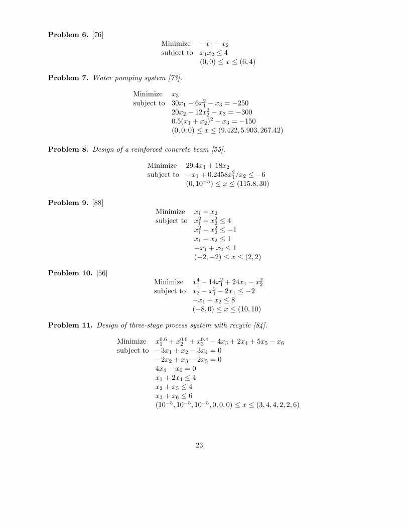
Problem 6. [76]Minimize −x1 − x2

subject to x1x2 ≤ 4(0, 0) ≤ x ≤ (6, 4)

Problem 7. Water pumping system [73].

Minimize x3

subject to 30x1 − 6x21 − x3 = −250

20x2 − 12x22 − x3 = −300

0.5(x1 + x2)2 − x3 = −150

(0, 0, 0) ≤ x ≤ (9.422, 5.903, 267.42)

Problem 8. Design of a reinforced concrete beam [55].

Minimize 29.4x1 + 18x2

subject to −x1 + 0.2458x21/x2 ≤ −6

(0, 10−5) ≤ x ≤ (115.8, 30)

Problem 9. [88]Minimize x1 + x2

subject to x21 + x2

2 ≤ 4x2

1 − x22 ≤ −1

x1 − x2 ≤ 1−x1 + x2 ≤ 1(−2,−2) ≤ x ≤ (2, 2)

Problem 10. [56]Minimize x4

1 − 14x21 + 24x1 − x2

2

subject to x2 − x21 − 2x1 ≤ −2

−x1 + x2 ≤ 8(−8, 0) ≤ x ≤ (10, 10)

Problem 11. Design of three-stage process system with recycle [84].

Minimize x0.61 + x0.6

2 + x0.43 − 4x3 + 2x4 + 5x5 − x6

subject to −3x1 + x2 − 3x4 = 0−2x2 + x3 − 2x5 = 04x4 − x6 = 0x1 + 2x4 ≤ 4x2 + x5 ≤ 4x3 + x6 ≤ 6(10−5, 10−5, 10−5, 0, 0, 0) ≤ x ≤ (3, 4, 4, 2, 2, 6)

23

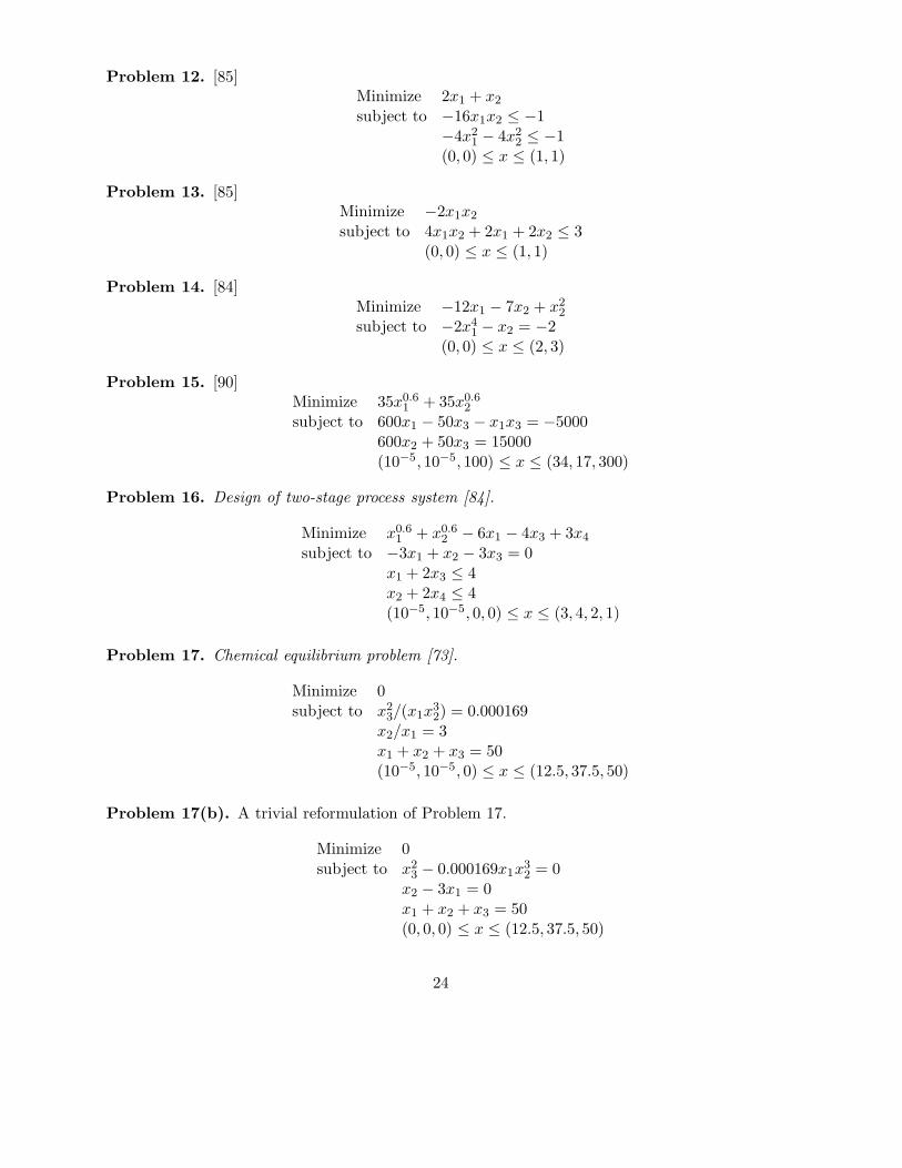
Problem 12. [85]Minimize 2x1 + x2

subject to −16x1x2 ≤ −1−4x2

1 − 4x22 ≤ −1

(0, 0) ≤ x ≤ (1, 1)

Problem 13. [85]Minimize −2x1x2

subject to 4x1x2 + 2x1 + 2x2 ≤ 3(0, 0) ≤ x ≤ (1, 1)

Problem 14. [84]Minimize −12x1 − 7x2 + x2

2

subject to −2x41 − x2 = −2

(0, 0) ≤ x ≤ (2, 3)

Problem 15. [90]Minimize 35x0.6

1 + 35x0.62

subject to 600x1 − 50x3 − x1x3 = −5000600x2 + 50x3 = 15000(10−5, 10−5, 100) ≤ x ≤ (34, 17, 300)

Problem 16. Design of two-stage process system [84].

Minimize x0.61 + x0.6

2 − 6x1 − 4x3 + 3x4

subject to −3x1 + x2 − 3x3 = 0x1 + 2x3 ≤ 4x2 + 2x4 ≤ 4(10−5, 10−5, 0, 0) ≤ x ≤ (3, 4, 2, 1)

Problem 17. Chemical equilibrium problem [73].

Minimize 0subject to x2

3/(x1x32) = 0.000169

x2/x1 = 3x1 + x2 + x3 = 50(10−5, 10−5, 0) ≤ x ≤ (12.5, 37.5, 50)

Problem 17(b). A trivial reformulation of Problem 17.

Minimize 0subject to x2

3 − 0.000169x1x32 = 0

x2 − 3x1 = 0x1 + x2 + x3 = 50(0, 0, 0) ≤ x ≤ (12.5, 37.5, 50)

24

Problem 18. Heat exchanger network design [55].

Minimize x1 + x2 + x3

subject to (x4 − 1)− 12x1(3− x4) = 0(x5 − x4)− 8x2(4− x5) = 0(5− x5)− 4x3 = 0(0, 0, 0, 1, 1) ≤ x ≤ (1.5834, 3.6250, 1, 3, 4)

25