ASTRONOMY & ASTROPHYSICS MARCH I 1999, PAGE 273

SUPPLEMENT SERIES

Astron. Astrophys. Suppl. Ser. 135, 273–289 (1999)

Gigahertz Peaked Spectrum sources from theJodrell Bank–VLA Astrometric Survey

I. Sources in the region 35� ≤ δ ≤ 75�

A. Marecki1, H. Falcke2, J. Niezgoda1, S.T. Garrington3, and A.R. Patnaik2

1 Centre for Astronomy, N. Copernicus University, ul. Gagarina 11, PL-87-100 Torun, Poland2 Max-Planck-Institut fur Radioastronomie, Auf dem Hugel 69, D-53121 Bonn, Germany3 Nuffield Radio Astronomy Laboratories, Jodrell Bank, Cheshire, SK11 9DL, UK

Received May 14; accepted October 13, 1998

Abstract. Observations with MERLIN1 at 408 MHz havebeen used to establish the low-frequency part of thespectra of more than a hundred compact radio sourcestaken from the part of the Jodrell Bank–VLA AstrometricSurvey limited by 35◦ ≤ δ ≤ 75◦. These sources wereselected from JVAS and other catalogues to have con-vex spectra between 1.4 and 8.4 GHz, characteristic ofGigahertz Peaked Spectrum (GPS) sources. We have con-firmed convex shapes of the spectra of 76 objects (onehalf of our initial candidates) thereby yielding the largestgenuine sample of GPS sources compiled so far. Seven of17 identified quasars in the sample have large (z >∼ 2)redshifts.

Key words: catalogs — galaxies: active — quasars:general — radio continuum: general

1. Introduction

By definition, Gigahertz Peaked Spectrum (GPS) sourceshave convex spectra with a turnover frequency νmax >1 GHz. It is generally accepted that such a spectral shaperesults from synchrotron self-absorption due to a highcompactness. Indeed, the linear sizes of GPS sources arevery small (10− 1000 pc) and their radio luminosities arelarge (Lradio ∼ 1045 erg/s). An important feature whichmakes the GPS class particularly interesting, is that GPSobjects identified with quasars often have very large red-shifts. A review on the properties of GPS sources has been

Send offprint requests to: H. Falcke,e-mail: hfalcke@mpifr-bonn.mpg.de

1 MERLIN is operated by The University of Manchester onbehalf of the UK Particle Physics and Astronomy ResearchCouncil.

given by O’Dea et al. (1991) — hereinafter OBS91 — andO’Dea (1998). De Vries et al. (1997) compiled spectra of72 GPS sources and constructed a canonical GPS radiospectrum. They found it to have a constant shape inde-pendent of AGN type, redshift or radio luminosity.

As Gopal-Krishna & Spoelstra (1993) pointed out,the great potential of GPS sources for discovering high-z objects continues to be the major motivation factor forenlarging the sample of GPS sources. A second motiva-tion for increasing the number of known GPS sourcescomes from the discovery (Wilkinson et al. 1994) of a newclass of Compact Symmetric Objects (CSO). Five archety-pal CSOs (cf. Readhead et al. 1996a) are all acknowl-edged GPS sources. Readhead et al. (1996b) argue thatCSOs are the young precursors of classical double radiosources. Increasing the list of known GPS sources offers apromising way to find more CSOs.

The search for GPS sources can be difficult because itrequires both high resolution and high sensitivity obser-vations at frequencies well below 1 GHz and high sensi-tivity observations at ν > 5 GHz, well above the poten-tial peak of the spectrum. Therefore, unlike in the caseof flat spectrum sources, only a modest number of GPSsources can simply be extracted from classical large cata-logues e.g. the Green Bank (GB) surveys at 1.4 GHz and4.85 GHz (White & Becker 1992 and references therein— hereinafter WB92) and the Texas Survey at 365 MHz(Douglas et al. 1996). For example, the sample ofStanghellini et al. (1990) was derived from the TexasSurvey and the 1 Jy catalogue of Kuhr et al. (1981a). Outof 55 sources and candidates they listed, 41 are currentlyacknowledged as GPS sources (O’Dea, priv. comm. 1996)and 33 make a complete sample (Stanghellini et al. 1996).

The lists published by Gopal-Krishna et al. (1983) andSpoelstra et al. (1985) resulting from dedicated observa-tions, e.g. with the Westerbork Synthesis Radio Telescope

274 A. Marecki et al.: Gigahertz Peaked Spectrum sources from the Jodrell Bank–VLA Astrometric Survey

(WSRT) or the Ooty telescope, are not very large: eachone contains 25 sources (5 and 2 out of these two sam-ples respectively had been retracted later). The sourcesgathered by the authors mentioned above have been col-lected in OBS91 in the so called “working sample” en-compassing 95 objects. Gopal-Krishna & Spoelstra (1993)confirmed the existence of 10 GPS sources and Cersosimoet al. (1994) found 7 more2. On the other hand 6 sourcesfrom the list in OBS91, namely 0218+357, 0528+134,0902+490, 1851+488, 2053−201 and 2230+114 proved tobe “not so good” examples of the class and have been re-tracted. By the end of 1997 very few other GPS sourceshad been discovered.

There are two ways to achieve a “bulk” increase ofthis number. The first one has been followed by Snellenet al. (1998) — hereinafter SSB98 — the second is thebasis of this paper. The former one is based on theWesterbork Northern Sky Survey (WENSS) being car-ried out with WSRT at 325 and 609 MHz. Naturally, thesources with inverted spectra in the WENSS are GPS can-didates, which are followed up with observations at higherfrequencies. This survey is particularly useful since it isthe most sensitive survey at low frequencies (more thanan order of magnitude better than the Texas Survey).

The published part of WENSS called “mini–survey”(Rengelink et al. 1997) is limited to 14h10m < α <20h30m, 57◦ < δ < 72◦50′ and covers ∼570 square de-grees only, so there are still large parts of the sky wherethis method cannot be applied. Nevertheless, SSB98 us-ing the mini–survey plus an unpublished part of WENSS(4h < α < 8h30m, the same declination range as the mini–survey) were able to establish a list of 47 “new” GPSsources.

2. Construction of the sample

Since WENSS was not available when our programmestarted in 1994, we adopted a different approach whichcan be regarded as “opposite” to that of SSB98 be-cause we started at the high frequencies end insteadof the low one. Hence, to determine candidate GPSsources, we used 8.4 GHz fluxes from the first part of theJodrell Bank–VLA Astrometric Survey (JVAS)3 (Patnaiket al. 1992) containing all compact radio sources in therange 35◦ ≤ δ ≤ 75◦ with fluxes > 200 mJy at 5 GHz. Wecombined them with 1.4 GHz and 4.85 GHz fluxes fromthe GB catalogues (WB92). For 32 sources 1.4 GHz fluxeswere missing in WB92 so we substituted them with thecatalogue flux density limit. Then we fitted the data witha second order polynomial of the form:

logSν = S0 + α log ν − c(log ν)2, (1)

2 Cersosimo et al. claim to discover more sources but only7 have been finally recognised as GPS.

3 JVAS resulted from observations made with the VLA in“A” configuration.

Table 1. Subsample One

IAUname R.A. Dec. Opt.(B1950) (J2000) ID

0059+581 01 02 45.7630 58 24 11.139 CW0102+480 01 05 49.9295 48 19 03.183 EF0627+532 06 31 34.6860 53 11 27.754 BS0652+426 06 56 10.6629 42 37 02.751 G0652+577 06 57 12.5027 57 41 56.740 EF0750+535 07 54 15.2177 53 24 56.450 EF0828+493 08 32 23.2171 49 13 21.036 BL1107+485 11 10 36.3237 48 17 52.446 EF1239+552 12 41 27.7043 54 58 19.040 EF1256+546 12 58 15.6078 54 21 52.112 EF1311+552 13 13 37.8518 54 58 23.894 EF1428+422 14 30 23.7418 42 04 36.503 EF1532+680 15 32 43.3426 67 55 13.992 EF1602+576 16 03 55.9311 57 30 54.415 BS1627+476 16 28 37.5064 47 34 10.414 BS1630+358 16 32 31.2578 35 47 37.740 EF1745+670 17 45 54.3577 67 03 49.302 EF1755+578 17 56 03.6285 57 48 47.990 BS1815+614 18 15 36.7920 61 27 11.641 EF1946+708 19 45 53.5197 70 55 48.723 ?2253+417 22 55 36.7082 42 02 52.535 BS2310+385 23 12 58.7950 38 47 42.668 BS2323+478 23 25 44.9131 48 06 25.280 BS2356+385 23 59 33.1809 38 50 42.322 BS

Explanation of ID field:

BL: BL Lac objectBS: blue stell. obj. (without the spec. - basically a quasar)BG: blue galaxy?CW: crowded field - too many objects for a clean

identificationEF: empty fieldG: galaxyNS: neutral stell. obj. (same magn. in both E and O prints)OB: obscured fieldQ: quasarRS: red stellar object.

where ν is the observed frequency in GHz and Sν theflux density in mJy and selected the sources with convexspectral shapes. The criterion for selecting an initial list ofcandidate GPS sources was that the curvature c had to begreater than 1 with a peak in the spectrum in the observ-able range (the limit of c > 1 is rather conservative andincludes also spectra which are much flatter than those oftypical GPS sources). Admittedly, although this criterionseems to be conservative enough, a few sources fromthe OBS91 “working sample” which happen to be JVASmembers, and therefore have been fitted with polynomials(0018+729, 0248+430, 0552+398, 2015+657, 2021+614,2352+495), did not fulfill it. In the end, the c > 1 thresh-old was chosen as a good compromise, to produce areasonably sized sample for future observations.

A. Marecki et al.: Gigahertz Peaked Spectrum sources from the Jodrell Bank–VLA Astrometric Survey 275

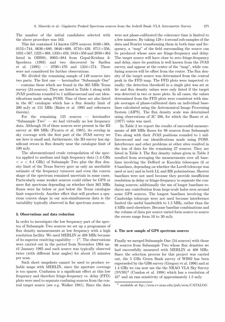
The number of the initial candidates selected withthe above procedure was 163.

This list contained 14 known GPS sources: 0108+388,0153+744, 0636+680, 0646+600, 0710+439, 0711+356,1031+567, 1225+368, 1333+459, 1843+356 and 2050+364listed in OBS91; 0903+684 from Gopal-Krishna &Spoelstra (1993) and two discovered by Snellenet al. (1995) — 0700+470 and 1324+574. Thesewere not considered for further observations.

We divided the remaining sample of 149 sources intotwo parts. The first one — hereinafter “Subsample One”— contains those which are found in the 365 MHz Texassurvey (24 sources). They are listed in Table 1 along withJVAS positions rounded to 1 milliarcsecond and our iden-tifications made using POSS. Nine of these are also listedin the 6C catalogue which has a flux density limit of200 mJy at 151 MHz (Hales et al. 1993 and referencestherein).

For the remaining 125 sources — hereinafter“Subsample Two” — we had virtually no low frequencydata. Although 19 of these sources were present in the B3survey at 408 MHz (Ficarra et al. 1985), its overlap insky coverage with the first part of the JVAS survey weuse here is small and, furthermore, the B3 survey has sig-nificant errors in flux density near the catalogue limit of100 mJy.

The aforementioned crude extrapolation of the spec-tra applied to medium and high frequency data (1.4 GHz< ν < 8.4 GHz) of Subsample Two plus the flux den-sity limit of the Texas Survey gave us only an unreliableestimate of the frequency turnover and even the convexshape of the spectrum remained uncertain in some cases.Particularly some weaker sources could either be GPS ormere flat spectrum depending on whether their 365 MHzfluxes were far below or just below the Texas cataloguelimit respectively. Another effect that will produce a spu-rious convex shape in our non-simultaneous data is thevariability typically observed in flat spectrum sources.

3. Observations and data reduction

In order to investigate the low frequency part of the spec-tra of Subsample Two sources we set up a programme offlux density measurements at low frequency with a highresolution facility. We used MERLIN at 408 MHz becauseof its superior resolving capability — 1′′. The observationswere carried out in the period from November 1994 un-til January 1995 and each source was typically observedtwice (with different hour angles) for about 15 minutesper scan.

Such short snapshots cannot be used to produce re-liable maps with MERLIN, since the aperture coverageis too sparse. Confusion is a significant effect at this lowfrequency and therefore fringe-frequency vs. delay (FFD)plots were used to separate confusing sources from the cen-tral target source (see e.g. Walker 1981). Since the data

were not phase-calibrated the coherence time is limited toa few minutes. By taking 128×4 second sub-samples of thedata and Fourier transforming them in both time and fre-quency, a “map” of the field surrounding the source canbe produced whose axes are fringe-frequency and delay.The target source will have close to zero fringe-frequencyand delay, since its position is well known from the JVASsurvey, and appear at the centre of the “map”, while con-fusing sources will be offset from the centre. The flux den-sity of the target source was determined from the centralpeak in the FFD map. The FFD plots were inspected vi-sually; the detection threshold in a single plot was set at3σ and flux density values were only listed if the targetwas detected in two or more plots. In all cases, the valuesdetermined from the FFD plots were consistent with sim-ple averages of phase-calibrated data on individual base-lines calculated using the Astronomical Image ProcessingSystem (AIPS). The flux density scale was determinedusing observations of 3C 286, for which the Baars et al.(1977) value was used.

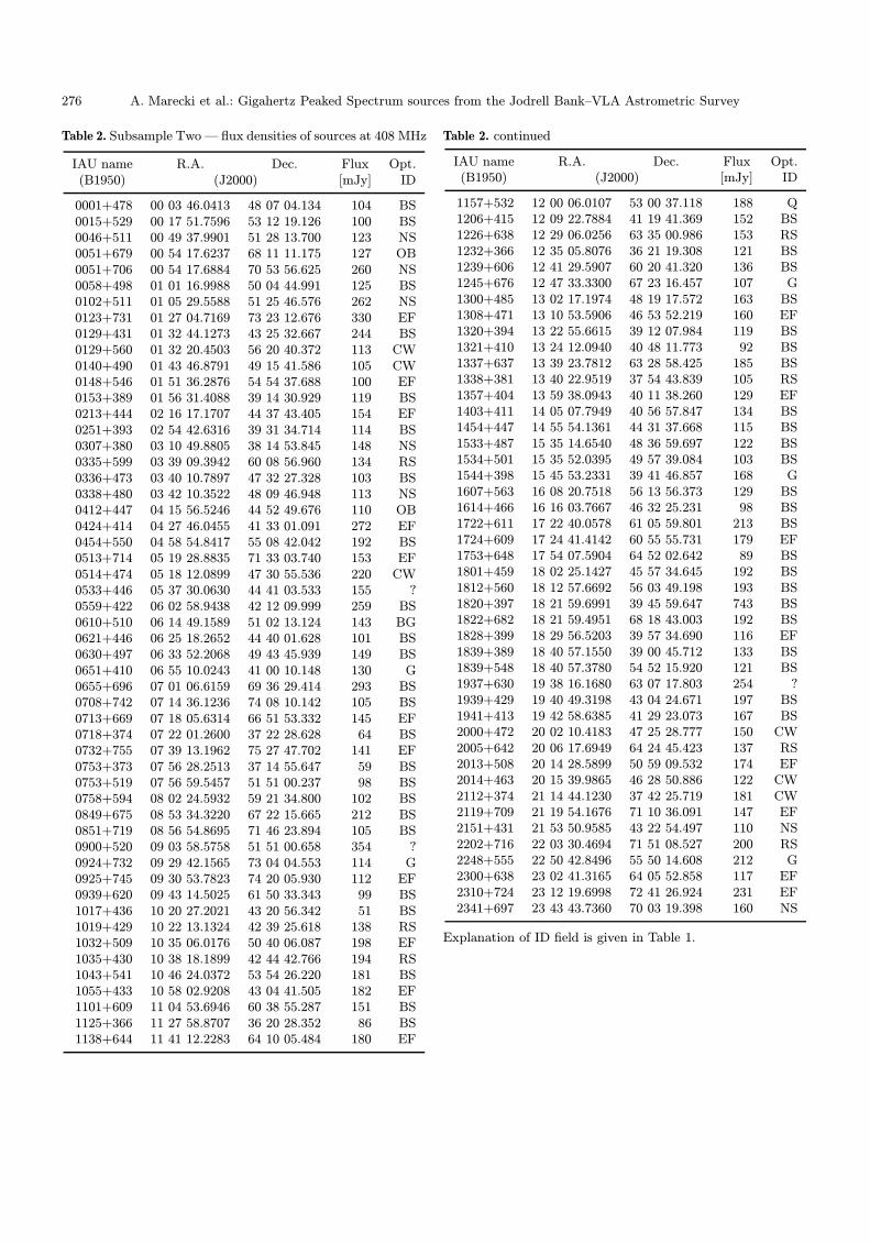
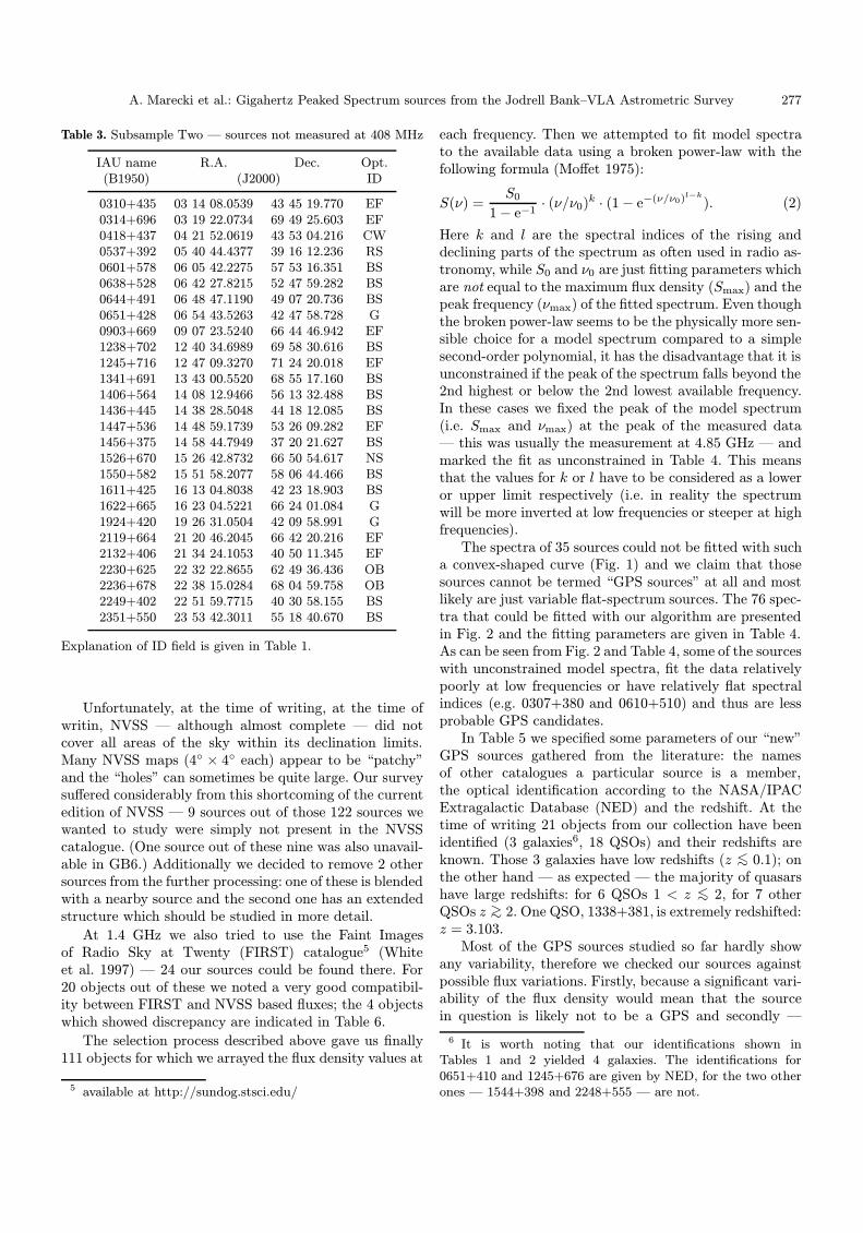
In Table 2 we report the results of successful measure-ments of 408 MHz fluxes for 98 sources from SubsampleTwo along with their JVAS positions rounded to 1 mil-liarcsecond and our identifications made using POSS.Interference and other problems at other sites resulted inthe loss of data for the remaining 27 sources. They arelisted in Table 3. The flux density values given in Table 2resulted from averaging the measurements over all base-lines involving the Defford or Knockin telescopes (6 or8 baselines, depending on whether the Lovell telescope wasused or not) and in both LL and RR polarisations. Shorterbaselines were not used because they provide insufficientresolution in delay or fringe-frequency to separate the con-fusing sources; additionally the use of longer baselines re-duces any contribution from large-scale halos seen aroundsome GPS sources. The longest baselines involving theCambridge telescope were not used because interferencelimited the useful bandwidth to 1.5 MHz, rather than the4 MHz used elsewhere. Because baseline combinations andthe volume of data per source varied form source to sourcethe errors range form 10 to 30 mJy.

4. The new sample of GPS spectrum sources

Finally we merged Subsample One (24 sources) with those98 sources from Subsample Two whose flux densities wehad successfully measured with MERLIN at 408 MHz.Since the selection process for this project was carriedout, the 5 GHz Green Bank survey of WB92 has beensuperseded by the GB6 survey (Gregory et al. 1996) and at1.4 GHz we can now use the the NRAO VLA Sky Survey(NVSS)4 (Condon et al. 1998) which has a resolution of45′′ and an rms sensitivity of approximately 1.5 mJy.

4 available at ftp://nvss.cv.nrao.edu/pub/nvss/CATALOG

276 A. Marecki et al.: Gigahertz Peaked Spectrum sources from the Jodrell Bank–VLA Astrometric Survey

Table 2. Subsample Two — flux densities of sources at 408 MHz

IAU name R.A. Dec. Flux Opt.(B1950) (J2000) [mJy] ID

0001+478 00 03 46.0413 48 07 04.134 104 BS0015+529 00 17 51.7596 53 12 19.126 100 BS0046+511 00 49 37.9901 51 28 13.700 123 NS0051+679 00 54 17.6237 68 11 11.175 127 OB0051+706 00 54 17.6884 70 53 56.625 260 NS0058+498 01 01 16.9988 50 04 44.991 125 BS0102+511 01 05 29.5588 51 25 46.576 262 NS0123+731 01 27 04.7169 73 23 12.676 330 EF0129+431 01 32 44.1273 43 25 32.667 244 BS0129+560 01 32 20.4503 56 20 40.372 113 CW0140+490 01 43 46.8791 49 15 41.586 105 CW0148+546 01 51 36.2876 54 54 37.688 100 EF0153+389 01 56 31.4088 39 14 30.929 119 BS0213+444 02 16 17.1707 44 37 43.405 154 EF0251+393 02 54 42.6316 39 31 34.714 114 BS0307+380 03 10 49.8805 38 14 53.845 148 NS0335+599 03 39 09.3942 60 08 56.960 134 RS0336+473 03 40 10.7897 47 32 27.328 103 BS0338+480 03 42 10.3522 48 09 46.948 113 NS0412+447 04 15 56.5246 44 52 49.676 110 OB0424+414 04 27 46.0455 41 33 01.091 272 EF0454+550 04 58 54.8417 55 08 42.042 192 BS0513+714 05 19 28.8835 71 33 03.740 153 EF0514+474 05 18 12.0899 47 30 55.536 220 CW0533+446 05 37 30.0630 44 41 03.533 155 ?0559+422 06 02 58.9438 42 12 09.999 259 BS0610+510 06 14 49.1589 51 02 13.124 143 BG0621+446 06 25 18.2652 44 40 01.628 101 BS0630+497 06 33 52.2068 49 43 45.939 149 BS0651+410 06 55 10.0243 41 00 10.148 130 G0655+696 07 01 06.6159 69 36 29.414 293 BS0708+742 07 14 36.1236 74 08 10.142 105 BS0713+669 07 18 05.6314 66 51 53.332 145 EF0718+374 07 22 01.2600 37 22 28.628 64 BS0732+755 07 39 13.1962 75 27 47.702 141 EF0753+373 07 56 28.2513 37 14 55.647 59 BS0753+519 07 56 59.5457 51 51 00.237 98 BS0758+594 08 02 24.5932 59 21 34.800 102 BS0849+675 08 53 34.3220 67 22 15.665 212 BS0851+719 08 56 54.8695 71 46 23.894 105 BS0900+520 09 03 58.5758 51 51 00.658 354 ?0924+732 09 29 42.1565 73 04 04.553 114 G0925+745 09 30 53.7823 74 20 05.930 112 EF0939+620 09 43 14.5025 61 50 33.343 99 BS1017+436 10 20 27.2021 43 20 56.342 51 BS1019+429 10 22 13.1324 42 39 25.618 138 RS1032+509 10 35 06.0176 50 40 06.087 198 EF1035+430 10 38 18.1899 42 44 42.766 194 RS1043+541 10 46 24.0372 53 54 26.220 181 BS1055+433 10 58 02.9208 43 04 41.505 182 EF1101+609 11 04 53.6946 60 38 55.287 151 BS1125+366 11 27 58.8707 36 20 28.352 86 BS1138+644 11 41 12.2283 64 10 05.484 180 EF

Table 2. continued

IAU name R.A. Dec. Flux Opt.(B1950) (J2000) [mJy] ID

1157+532 12 00 06.0107 53 00 37.118 188 Q1206+415 12 09 22.7884 41 19 41.369 152 BS1226+638 12 29 06.0256 63 35 00.986 153 RS1232+366 12 35 05.8076 36 21 19.308 121 BS1239+606 12 41 29.5907 60 20 41.320 136 BS1245+676 12 47 33.3300 67 23 16.457 107 G1300+485 13 02 17.1974 48 19 17.572 163 BS1308+471 13 10 53.5906 46 53 52.219 160 EF1320+394 13 22 55.6615 39 12 07.984 119 BS1321+410 13 24 12.0940 40 48 11.773 92 BS1337+637 13 39 23.7812 63 28 58.425 185 BS1338+381 13 40 22.9519 37 54 43.839 105 RS1357+404 13 59 38.0943 40 11 38.260 129 EF1403+411 14 05 07.7949 40 56 57.847 134 BS1454+447 14 55 54.1361 44 31 37.668 115 BS1533+487 15 35 14.6540 48 36 59.697 122 BS1534+501 15 35 52.0395 49 57 39.084 103 BS1544+398 15 45 53.2331 39 41 46.857 168 G1607+563 16 08 20.7518 56 13 56.373 129 BS1614+466 16 16 03.7667 46 32 25.231 98 BS1722+611 17 22 40.0578 61 05 59.801 213 BS1724+609 17 24 41.4142 60 55 55.731 179 EF1753+648 17 54 07.5904 64 52 02.642 89 BS1801+459 18 02 25.1427 45 57 34.645 192 BS1812+560 18 12 57.6692 56 03 49.198 193 BS1820+397 18 21 59.6991 39 45 59.647 743 BS1822+682 18 21 59.4951 68 18 43.003 192 BS1828+399 18 29 56.5203 39 57 34.690 116 EF1839+389 18 40 57.1550 39 00 45.712 133 BS1839+548 18 40 57.3780 54 52 15.920 121 BS1937+630 19 38 16.1680 63 07 17.803 254 ?1939+429 19 40 49.3198 43 04 24.671 197 BS1941+413 19 42 58.6385 41 29 23.073 167 BS2000+472 20 02 10.4183 47 25 28.777 150 CW2005+642 20 06 17.6949 64 24 45.423 137 RS2013+508 20 14 28.5899 50 59 09.532 174 EF2014+463 20 15 39.9865 46 28 50.886 122 CW2112+374 21 14 44.1230 37 42 25.719 181 CW2119+709 21 19 54.1676 71 10 36.091 147 EF2151+431 21 53 50.9585 43 22 54.497 110 NS2202+716 22 03 30.4694 71 51 08.527 200 RS2248+555 22 50 42.8496 55 50 14.608 212 G2300+638 23 02 41.3165 64 05 52.858 117 EF2310+724 23 12 19.6998 72 41 26.924 231 EF2341+697 23 43 43.7360 70 03 19.398 160 NS

Explanation of ID field is given in Table 1.

A. Marecki et al.: Gigahertz Peaked Spectrum sources from the Jodrell Bank–VLA Astrometric Survey 277

Table 3. Subsample Two — sources not measured at 408 MHz

IAU name R.A. Dec. Opt.(B1950) (J2000) ID

0310+435 03 14 08.0539 43 45 19.770 EF0314+696 03 19 22.0734 69 49 25.603 EF0418+437 04 21 52.0619 43 53 04.216 CW0537+392 05 40 44.4377 39 16 12.236 RS0601+578 06 05 42.2275 57 53 16.351 BS0638+528 06 42 27.8215 52 47 59.282 BS0644+491 06 48 47.1190 49 07 20.736 BS0651+428 06 54 43.5263 42 47 58.728 G0903+669 09 07 23.5240 66 44 46.942 EF1238+702 12 40 34.6989 69 58 30.616 BS1245+716 12 47 09.3270 71 24 20.018 EF1341+691 13 43 00.5520 68 55 17.160 BS1406+564 14 08 12.9466 56 13 32.488 BS1436+445 14 38 28.5048 44 18 12.085 BS1447+536 14 48 59.1739 53 26 09.282 EF1456+375 14 58 44.7949 37 20 21.627 BS1526+670 15 26 42.8732 66 50 54.617 NS1550+582 15 51 58.2077 58 06 44.466 BS1611+425 16 13 04.8038 42 23 18.903 BS1622+665 16 23 04.5221 66 24 01.084 G1924+420 19 26 31.0504 42 09 58.991 G2119+664 21 20 46.2045 66 42 20.216 EF2132+406 21 34 24.1053 40 50 11.345 EF2230+625 22 32 22.8655 62 49 36.436 OB2236+678 22 38 15.0284 68 04 59.758 OB2249+402 22 51 59.7715 40 30 58.155 BS2351+550 23 53 42.3011 55 18 40.670 BS

Explanation of ID field is given in Table 1.

Unfortunately, at the time of writing, at the time ofwritin, NVSS — although almost complete — did notcover all areas of the sky within its declination limits.Many NVSS maps (4◦ × 4◦ each) appear to be “patchy”and the “holes” can sometimes be quite large. Our surveysuffered considerably from this shortcoming of the currentedition of NVSS — 9 sources out of those 122 sources wewanted to study were simply not present in the NVSScatalogue. (One source out of these nine was also unavail-able in GB6.) Additionally we decided to remove 2 othersources from the further processing: one of these is blendedwith a nearby source and the second one has an extendedstructure which should be studied in more detail.

At 1.4 GHz we also tried to use the Faint Imagesof Radio Sky at Twenty (FIRST) catalogue5 (Whiteet al. 1997) — 24 our sources could be found there. For20 objects out of these we noted a very good compatibil-ity between FIRST and NVSS based fluxes; the 4 objectswhich showed discrepancy are indicated in Table 6.

The selection process described above gave us finally111 objects for which we arrayed the flux density values at

5 available at http://sundog.stsci.edu/

each frequency. Then we attempted to fit model spectrato the available data using a broken power-law with thefollowing formula (Moffet 1975):

S(ν) =S0

1− e−1· (ν/ν0)k · (1− e−(ν/ν0)l−k). (2)

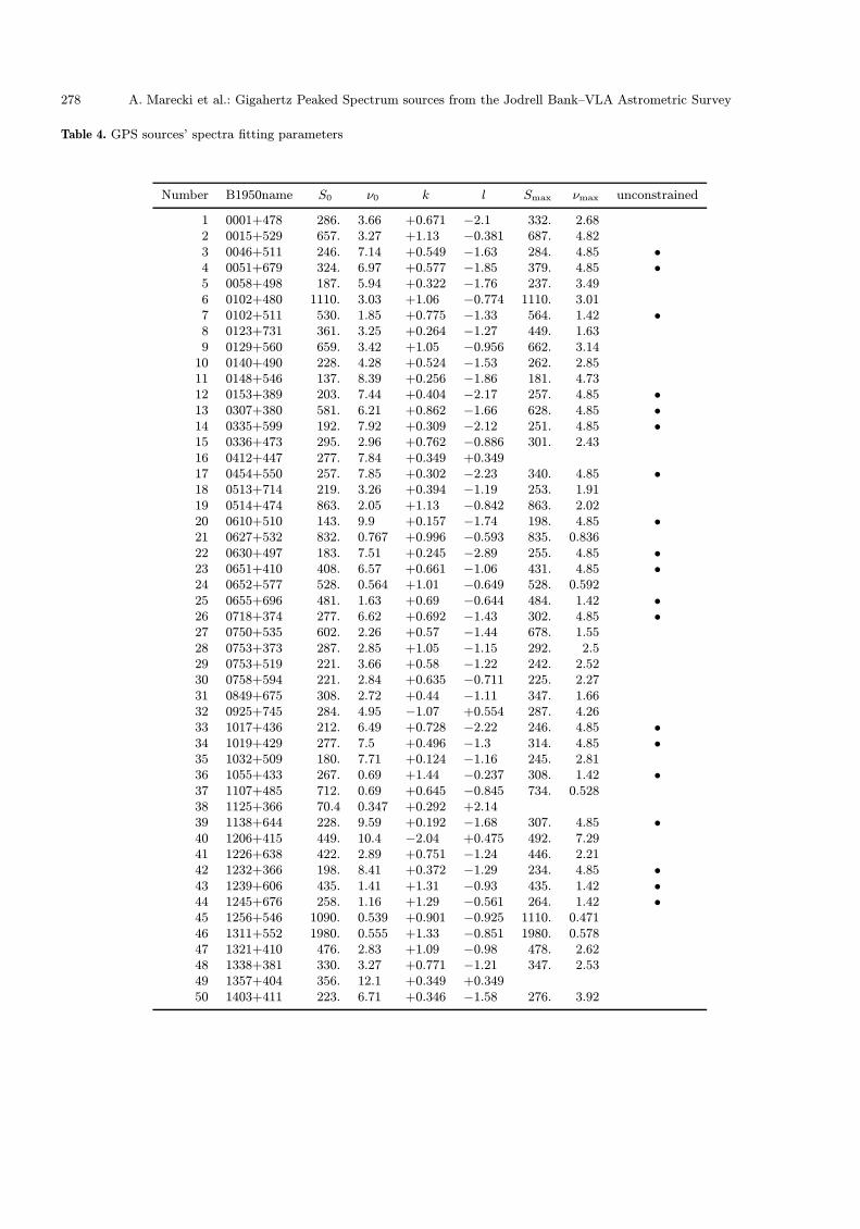
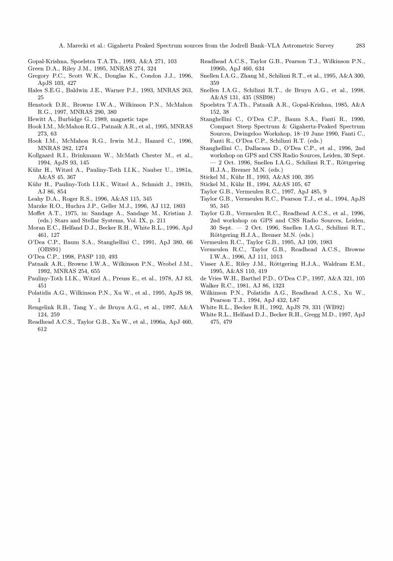
Here k and l are the spectral indices of the rising anddeclining parts of the spectrum as often used in radio as-tronomy, while S0 and ν0 are just fitting parameters whichare not equal to the maximum flux density (Smax) and thepeak frequency (νmax) of the fitted spectrum. Even thoughthe broken power-law seems to be the physically more sen-sible choice for a model spectrum compared to a simplesecond-order polynomial, it has the disadvantage that it isunconstrained if the peak of the spectrum falls beyond the2nd highest or below the 2nd lowest available frequency.In these cases we fixed the peak of the model spectrum(i.e. Smax and νmax) at the peak of the measured data— this was usually the measurement at 4.85 GHz — andmarked the fit as unconstrained in Table 4. This meansthat the values for k or l have to be considered as a loweror upper limit respectively (i.e. in reality the spectrumwill be more inverted at low frequencies or steeper at highfrequencies).

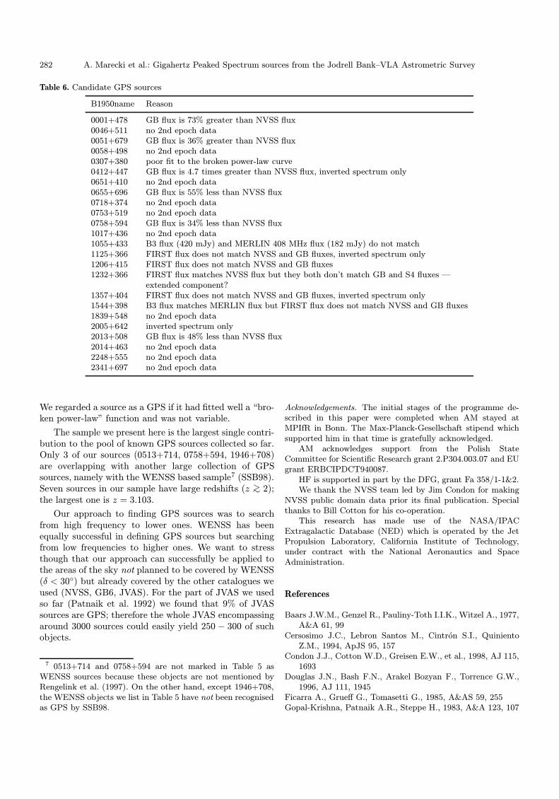
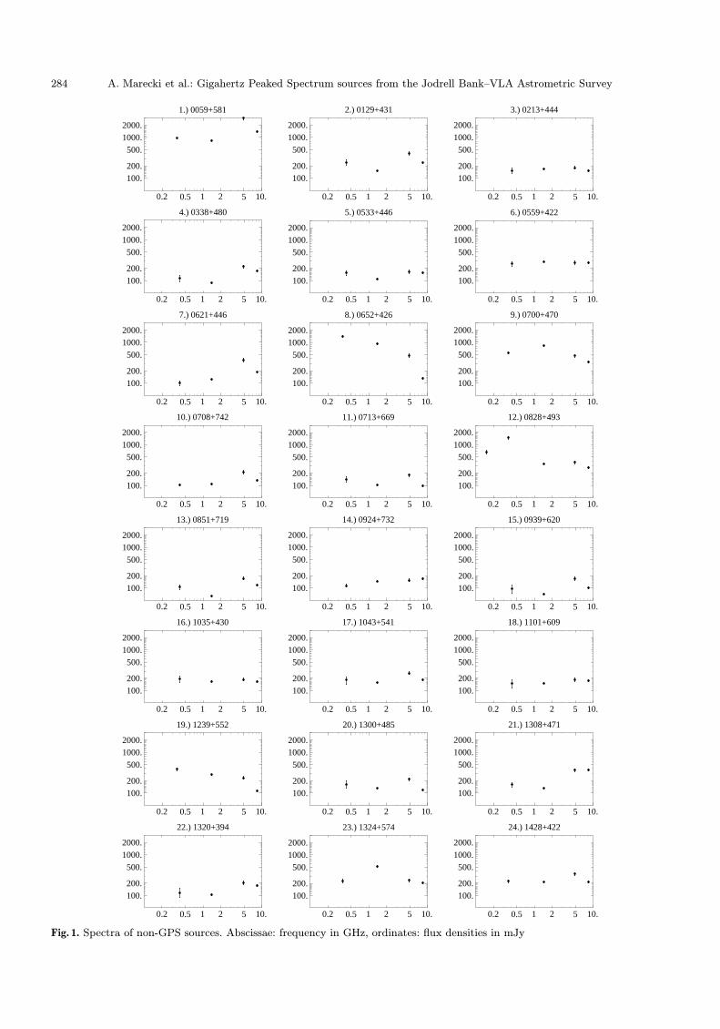
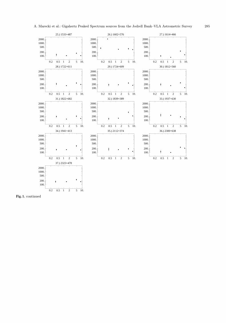
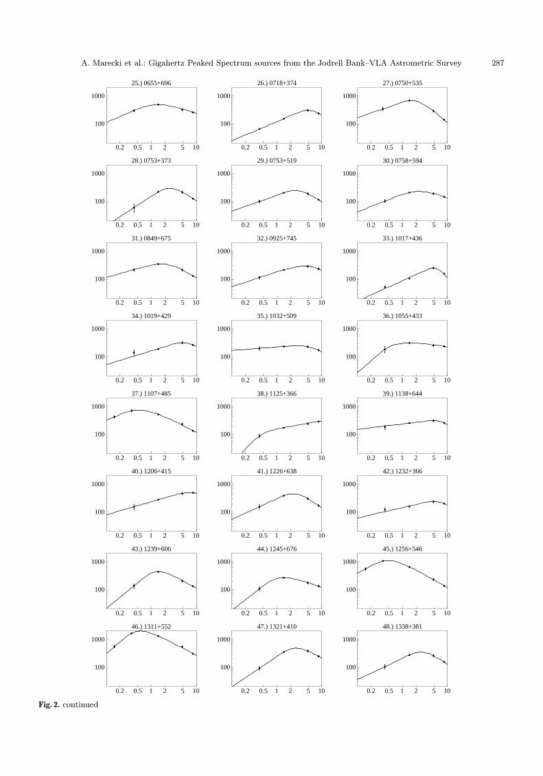
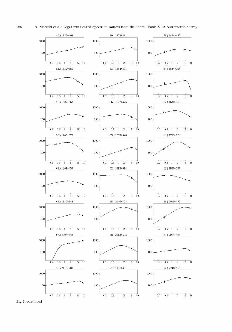
The spectra of 35 sources could not be fitted with sucha convex-shaped curve (Fig. 1) and we claim that thosesources cannot be termed “GPS sources” at all and mostlikely are just variable flat-spectrum sources. The 76 spec-tra that could be fitted with our algorithm are presentedin Fig. 2 and the fitting parameters are given in Table 4.As can be seen from Fig. 2 and Table 4, some of the sourceswith unconstrained model spectra, fit the data relativelypoorly at low frequencies or have relatively flat spectralindices (e.g. 0307+380 and 0610+510) and thus are lessprobable GPS candidates.

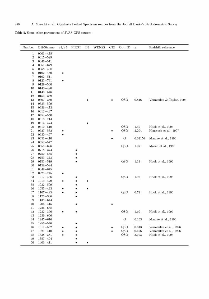
In Table 5 we specified some parameters of our “new”GPS sources gathered from the literature: the namesof other catalogues a particular source is a member,the optical identification according to the NASA/IPACExtragalactic Database (NED) and the redshift. At thetime of writing 21 objects from our collection have beenidentified (3 galaxies6, 18 QSOs) and their redshifts areknown. Those 3 galaxies have low redshifts (z <∼ 0.1); onthe other hand — as expected — the majority of quasarshave large redshifts: for 6 QSOs 1 < z <∼ 2, for 7 otherQSOs z >∼ 2. One QSO, 1338+381, is extremely redshifted:z = 3.103.

Most of the GPS sources studied so far hardly showany variability, therefore we checked our sources againstpossible flux variations. Firstly, because a significant vari-ability of the flux density would mean that the sourcein question is likely not to be a GPS and secondly —

6 It is worth noting that our identifications shown inTables 1 and 2 yielded 4 galaxies. The identifications for0651+410 and 1245+676 are given by NED, for the two otherones — 1544+398 and 2248+555 — are not.

278 A. Marecki et al.: Gigahertz Peaked Spectrum sources from the Jodrell Bank–VLA Astrometric Survey

Table 4. GPS sources’ spectra fitting parameters

Number B1950name S0 ν0 k l Smax νmax unconstrained

1 0001+478 286. 3.66 +0.671 −2.1 332. 2.682 0015+529 657. 3.27 +1.13 −0.381 687. 4.823 0046+511 246. 7.14 +0.549 −1.63 284. 4.85 •4 0051+679 324. 6.97 +0.577 −1.85 379. 4.85 •5 0058+498 187. 5.94 +0.322 −1.76 237. 3.496 0102+480 1110. 3.03 +1.06 −0.774 1110. 3.017 0102+511 530. 1.85 +0.775 −1.33 564. 1.42 •8 0123+731 361. 3.25 +0.264 −1.27 449. 1.639 0129+560 659. 3.42 +1.05 −0.956 662. 3.14

10 0140+490 228. 4.28 +0.524 −1.53 262. 2.8511 0148+546 137. 8.39 +0.256 −1.86 181. 4.7312 0153+389 203. 7.44 +0.404 −2.17 257. 4.85 •13 0307+380 581. 6.21 +0.862 −1.66 628. 4.85 •14 0335+599 192. 7.92 +0.309 −2.12 251. 4.85 •15 0336+473 295. 2.96 +0.762 −0.886 301. 2.4316 0412+447 277. 7.84 +0.349 +0.34917 0454+550 257. 7.85 +0.302 −2.23 340. 4.85 •18 0513+714 219. 3.26 +0.394 −1.19 253. 1.9119 0514+474 863. 2.05 +1.13 −0.842 863. 2.0220 0610+510 143. 9.9 +0.157 −1.74 198. 4.85 •21 0627+532 832. 0.767 +0.996 −0.593 835. 0.83622 0630+497 183. 7.51 +0.245 −2.89 255. 4.85 •23 0651+410 408. 6.57 +0.661 −1.06 431. 4.85 •24 0652+577 528. 0.564 +1.01 −0.649 528. 0.59225 0655+696 481. 1.63 +0.69 −0.644 484. 1.42 •26 0718+374 277. 6.62 +0.692 −1.43 302. 4.85 •27 0750+535 602. 2.26 +0.57 −1.44 678. 1.5528 0753+373 287. 2.85 +1.05 −1.15 292. 2.529 0753+519 221. 3.66 +0.58 −1.22 242. 2.5230 0758+594 221. 2.84 +0.635 −0.711 225. 2.2731 0849+675 308. 2.72 +0.44 −1.11 347. 1.6632 0925+745 284. 4.95 −1.07 +0.554 287. 4.2633 1017+436 212. 6.49 +0.728 −2.22 246. 4.85 •34 1019+429 277. 7.5 +0.496 −1.3 314. 4.85 •35 1032+509 180. 7.71 +0.124 −1.16 245. 2.8136 1055+433 267. 0.69 +1.44 −0.237 308. 1.42 •37 1107+485 712. 0.69 +0.645 −0.845 734. 0.52838 1125+366 70.4 0.347 +0.292 +2.1439 1138+644 228. 9.59 +0.192 −1.68 307. 4.85 •40 1206+415 449. 10.4 −2.04 +0.475 492. 7.2941 1226+638 422. 2.89 +0.751 −1.24 446. 2.2142 1232+366 198. 8.41 +0.372 −1.29 234. 4.85 •43 1239+606 435. 1.41 +1.31 −0.93 435. 1.42 •44 1245+676 258. 1.16 +1.29 −0.561 264. 1.42 •45 1256+546 1090. 0.539 +0.901 −0.925 1110. 0.47146 1311+552 1980. 0.555 +1.33 −0.851 1980. 0.57847 1321+410 476. 2.83 +1.09 −0.98 478. 2.6248 1338+381 330. 3.27 +0.771 −1.21 347. 2.5349 1357+404 356. 12.1 +0.349 +0.34950 1403+411 223. 6.71 +0.346 −1.58 276. 3.92

A. Marecki et al.: Gigahertz Peaked Spectrum sources from the Jodrell Bank–VLA Astrometric Survey 279

Table 4. continued

Number B1950name S0 ν0 k l Smax νmax unconstrained

51 1454+447 206. 2.36 +0.588 −0.407 206. 2.4352 1532+680 455. 2.57 +0.329 −1.32 551. 1.42 •53 1534+501 341. 6.97 +0.584 −1.09 367. 4.85 •54 1544+398 221. 6.4 +0.363 −4.67 310. 4.85 •55 1607+563 261. 3.54 +0.538 −0.797 273. 2.4856 1627+476 219. 3.06 +0.241 −1.11 271. 1.42 •57 1630+358 466. 2.5 +0.377 −1.11 537. 1.42 •58 1745+670 548. 2.7 +0.266 −1.46 696. 1.42 •59 1753+648 220. 7.26 +0.519 −1.66 257. 4.85 •60 1755+578 785. 2.07 +1.06 −1.07 793. 1.8661 1801+459 231. 2.78 +0.337 −0.77 256. 1.4662 1815+614 580. 3.9 +0.0731 −1.69 852. 1.6163 1820+397 753. 0.457 −0.519 +0.527 761. 0.57564 1839+548 240. 5.62 +0.436 −0.983 265. 3.4265 1946+708 965. 1.92 +0.818 −0.755 970. 1.7266 2000+472 946. 4.11 +0.996 −0.588 949. 4.5167 2005+642 227. 0.502 +0.346 +3.468 2013+508 363. 1.67 +0.849 −0.927 369. 1.42 •69 2014+463 153. 8.03 +0.231 −1.88 205. 4.4470 2119+709 167. 9.07 +0.217 −1.79 224. 4.85 •71 2151+431 257. 3.25 +0.63 −0.917 268. 2.4172 2248+555 469. 4.72 +0.512 −0.633 481. 3.4373 2253+417 1840. 1.83 +0.706 −0.909 1900. 1.4474 2310+385 682. 3.2 +0.6 −1.14 735. 2.2575 2341+697 155. 7.5 +0.147 −1.59 213. 3.4576 2356+385 560. 3.85 +0.524 −1.34 632. 2.55

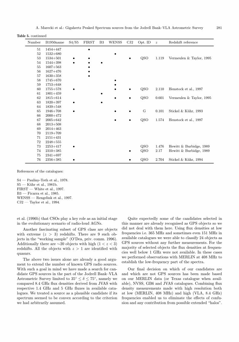
since our data are not simultaneous — any variabilitymakes derivation of spectra questionable. The part ofsources’ spectra around 1.4 GHz is obviously the most“sensitive” with regard to the GPS phenomenon so wecompared fluxes at this frequency given in WB92 tothose from NVSS. We applied corrections for the dif-ferent beam sizes of these two measurements. If a par-ticular source had changed its flux between epochs ofthe GB surveys and NVSS/FIRST more than 25% orthe 1.4 GHz GB flux was missing in WB92 we treatedsuch a source as potentially variable, unless we couldfind a second epoch flux density measurement else-where. We assigned a “candidate” status for such ob-jects and listed them in Table 6. Among these there are4 sources (0412+447, 1125+366, 1357+404, 2005+642)with inverted spectra only, i.e. apparently havingturnovers in their spectra at frequencies larger than8.4 GHz. This feature was yet another reason to assignthem a candidate status.

5. Notes on individual sources

Apart from the information in Table 5 we note that:

– 0627+532, 0652+577, 1107+485, 1256+546 and1311+552 are 6C sources (Hales et al. 1993 and ref-erences therein).

– 1107+485 is a member of the DRAO 408 MHz survey(Green & Riley 1995).

– 1745+670 and 1753+648 are members of the NEPsurvey (Kollgaard et al. 1994).

– 1607+563, 1755+578 and 1815+614 are members ofthe 7C survey (Visser et al. 1995).

– 0514+474 was observed by Leahy & Roger (1996).– 0102+480 and 2253+417 are members of the CJ1 sur-

vey (Polatidis et al. 1995).– 1245+676 is a giant radio galaxy with a GPS core

(O’Dea priv. comm. 1996).– 0140+490 has a large scale symmetric structure 2.′5

across.– 1839+548 and 2119+709 are marked as “quasi-point”

sources in JVAS. All other sources are pointlike i.e.they are unresolved by the VLA in “A” configurationat 8.4 GHz.

– 1815+614 and 1946+708 are CSOs (Taylor et al. 1996;Taylor & Vermeulen 1997).

6. Summary

Gigahertz Peaked Spectrum objects are an astrophysicallysignificant and important class yet they are still not wellunderstood (O’Dea 1998). They are not necessarily a uni-form class, and one can easily name subclasses among thewhole GPS ensemble. For example CSOs make one welldefined group — all of them are GPS galaxies with char-acteristic VLBI morphologies. It is claimed by Readhead

280 A. Marecki et al.: Gigahertz Peaked Spectrum sources from the Jodrell Bank–VLA Astrometric Survey

Table 5. Some other parameters of JVAS GPS sources

Number B1950name S4/S5 FIRST B3 WENSS CJ2 Opt. ID z Redshift reference

1 0001+4782 0015+5293 0046+5114 0051+6795 0058+4986 0102+480 •7 0102+5118 0123+731 •9 0129+560

10 0140+49011 0148+54612 0153+38913 0307+380 • • QSO 0.816 Vermeulen & Taylor, 199514 0335+59915 0336+47316 0412+44717 0454+55018 0513+71419 0514+474 •20 0610+510 QSO 1.59 Hook et al., 199621 0627+532 • • QSO 2.204 Henstock et al., 199722 0630+497 •23 0651+410 • G 0.02156 Marzke et al., 199624 0652+57725 0655+696 QSO 1.971 Moran et al., 199626 0718+374 •27 0750+535 •28 0753+373 •29 0753+519 • QSO 1.33 Hook et al., 199630 0758+59431 0849+67532 0925+745 •33 1017+436 • QSO 1.96 Hook et al., 199634 1019+429 • • •35 1032+509 •36 1055+433 • • •37 1107+485 • • QSO 0.74 Hook et al., 199638 1125+366 •39 1138+64440 1206+415 • •41 1226+63842 1232+366 • • QSO 1.60 Hook et al., 199643 1239+60644 1245+676 G 0.103 Marzke et al., 199645 1256+546 •46 1311+552 • • • QSO 0.613 Vermeulen et al., 199647 1321+410 • • • QSO 0.496 Vermeulen et al., 199648 1338+381 • • QSO 3.103 Hook et al., 199549 1357+404 •50 1403+411 • •

A. Marecki et al.: Gigahertz Peaked Spectrum sources from the Jodrell Bank–VLA Astrometric Survey 281

Table 5. continued

Number B1950name S4/S5 FIRST B3 WENSS CJ2 Opt. ID z Redshift reference

51 1454+447 •52 1532+680 •53 1534+501 • • • QSO 1.119 Vermeulen & Taylor, 199554 1544+398 • • •55 1607+563 •56 1627+476 •57 1630+358 •58 1745+670 •59 1753+648 •60 1755+578 • • • QSO 2.110 Henstock et al., 199761 1801+459 •62 1815+614 • • QSO 0.601 Vermeulen & Taylor, 199563 1820+397 • •64 1839+54865 1946+708 • • • G 0.101 Stickel & Kuhr, 199366 2000+47267 2005+642 • • QSO 1.574 Henstock et al., 199768 2013+50869 2014+46370 2119+70971 2151+43172 2248+55573 2253+417 • QSO 1.476 Hewitt & Burbidge, 198974 2310+385 • QSO 2.17 Hewitt & Burbidge, 198975 2341+69776 2356+385 • • QSO 2.704 Stickel & Kuhr, 1994

References of the catalogues:

S4 — Pauliny-Toth et al., 1978.S5 — Kuhr et al., 1981b.FIRST — White et al., 1997.B3 — Ficarra et al., 1985.WENSS — Rengelink et al., 1997.CJ2 — Taylor et al., 1994.

et al. (1996b) that CSOs play a key role as an initial stagein the evolutionary scenario of radio-loud AGNs.

Another fascinating subset of GPS class are objectswith extreme (z > 3) redshifts. There are 9 such ob-jects in the “working sample” (O’Dea, priv. comm. 1996).Additionally there are ∼20 objects with high (1 < z < 3)redshifts. All the objects with z > 1 are identified withquasars.

The above two issues alone are already a good argu-ment to extend the number of known GPS radio sources.With such a goal in mind we have made a search for can-didate GPS sources in the part of the Jodrell Bank–VLAAstrometric Survey limited to 35◦ ≤ δ ≤ 75◦, namely wecompared 8.4 GHz flux densities derived from JVAS withrespective 1.4 GHz and 5 GHz fluxes in available cata-logues. We treated a source as a plausible candidate if itsspectrum seemed to be convex according to the criterionwe had arbitrarily assumed.

Quite expectedly some of the candidates selected inthis manner are already recognised as GPS objects so wedid not deal with them here. Using flux densities at lowfrequencies i.e. 365 MHz and sometimes even 151 MHz inavailable catalogues we were able to classify 24 objects asGPS sources without any further measurements. For themajority of selected objects the flux densities at frequen-cies well below 1 GHz were not available. In these caseswe performed observations with MERLIN at 408 MHz toestablish the low-frequency part of the spectra.

Our final decision on which of our candidates areand which are not GPS sources has been made basedon our MERLIN data (or Texas catalogue when avail-able), NVSS, GB6 and JVAS catalogues. Combining fluxdensity measurements made with high resolution bothat low (MERLIN, 408 MHz) and high (VLA, 8.4 GHz)frequencies enabled us to eliminate the effects of confu-sion and any contribution from possible extended “halos”.

282 A. Marecki et al.: Gigahertz Peaked Spectrum sources from the Jodrell Bank–VLA Astrometric Survey

Table 6. Candidate GPS sources

B1950name Reason

0001+478 GB flux is 73% greater than NVSS flux0046+511 no 2nd epoch data0051+679 GB flux is 36% greater than NVSS flux0058+498 no 2nd epoch data0307+380 poor fit to the broken power-law curve0412+447 GB flux is 4.7 times greater than NVSS flux, inverted spectrum only0651+410 no 2nd epoch data0655+696 GB flux is 55% less than NVSS flux0718+374 no 2nd epoch data0753+519 no 2nd epoch data0758+594 GB flux is 34% less than NVSS flux1017+436 no 2nd epoch data1055+433 B3 flux (420 mJy) and MERLIN 408 MHz flux (182 mJy) do not match1125+366 FIRST flux does not match NVSS and GB fluxes, inverted spectrum only1206+415 FIRST flux does not match NVSS and GB fluxes1232+366 FIRST flux matches NVSS flux but they both don’t match GB and S4 fluxes —

extended component?1357+404 FIRST flux does not match NVSS and GB fluxes, inverted spectrum only1544+398 B3 flux matches MERLIN flux but FIRST flux does not match NVSS and GB fluxes1839+548 no 2nd epoch data2005+642 inverted spectrum only2013+508 GB flux is 48% less than NVSS flux2014+463 no 2nd epoch data2248+555 no 2nd epoch data2341+697 no 2nd epoch data

We regarded a source as a GPS if it had fitted well a “bro-ken power-law” function and was not variable.

The sample we present here is the largest single contri-bution to the pool of known GPS sources collected so far.Only 3 of our sources (0513+714, 0758+594, 1946+708)are overlapping with another large collection of GPSsources, namely with the WENSS based sample7 (SSB98).Seven sources in our sample have large redshifts (z >∼ 2);the largest one is z = 3.103.

Our approach to finding GPS sources was to searchfrom high frequency to lower ones. WENSS has beenequally successful in defining GPS sources but searchingfrom low frequencies to higher ones. We want to stressthough that our approach can successfully be applied tothe areas of the sky not planned to be covered by WENSS(δ < 30◦) but already covered by the other catalogues weused (NVSS, GB6, JVAS). For the part of JVAS we usedso far (Patnaik et al. 1992) we found that 9% of JVASsources are GPS; therefore the whole JVAS encompassingaround 3000 sources could easily yield 250 − 300 of suchobjects.

7 0513+714 and 0758+594 are not marked in Table 5 asWENSS sources because these objects are not mentioned byRengelink et al. (1997). On the other hand, except 1946+708,the WENSS objects we list in Table 5 have not been recognisedas GPS by SSB98.

Acknowledgements. The initial stages of the programme de-scribed in this paper were completed when AM stayed atMPIfR in Bonn. The Max-Planck-Gesellschaft stipend whichsupported him in that time is gratefully acknowledged.

AM acknowledges support from the Polish StateCommittee for Scientific Research grant 2.P304.003.07 and EUgrant ERBCIPDCT940087.

HF is supported in part by the DFG, grant Fa 358/1-1&2.We thank the NVSS team led by Jim Condon for making

NVSS public domain data prior its final publication. Specialthanks to Bill Cotton for his co-operation.

This research has made use of the NASA/IPACExtragalactic Database (NED) which is operated by the JetPropulsion Laboratory, California Institute of Technology,under contract with the National Aeronautics and SpaceAdministration.

References

Baars J.W.M., Genzel R., Pauliny-Toth I.I.K., Witzel A., 1977,A&A 61, 99

Cersosimo J.C., Lebron Santos M., Cintron S.I., QuinientoZ.M., 1994, ApJS 95, 157

Condon J.J., Cotton W.D., Greisen E.W., et al., 1998, AJ 115,1693

Douglas J.N., Bash F.N., Arakel Bozyan F., Torrence G.W.,1996, AJ 111, 1945

Ficarra A., Grueff G., Tomasetti G., 1985, A&AS 59, 255Gopal-Krishna, Patnaik A.R., Steppe H., 1983, A&A 123, 107

A. Marecki et al.: Gigahertz Peaked Spectrum sources from the Jodrell Bank–VLA Astrometric Survey 283

Gopal-Krishna, Spoelstra T.A.Th., 1993, A&A 271, 103Green D.A., Riley J.M., 1995, MNRAS 274, 324Gregory P.C., Scott W.K., Douglas K., Condon J.J., 1996,

ApJS 103, 427Hales S.E.G., Baldwin J.E., Warner P.J., 1993, MNRAS 263,

25Henstock D.R., Browne I.W.A., Wilkinson P.N., McMahon

R.G., 1997, MNRAS 290, 380Hewitt A., Burbidge G., 1989, magnetic tapeHook I.M., McMahon R.G., Patnaik A.R., et al., 1995, MNRAS

273, 63Hook I.M., McMahon R.G., Irwin M.J., Hazard C., 1996,

MNRAS 282, 1274Kollgaard R.I., Brinkmann W., McMath Chester M., et al.,

1994, ApJS 93, 145Kuhr H., Witzel A., Pauliny-Toth I.I.K., Nauber U., 1981a,

A&AS 45, 367Kuhr H., Pauliny-Toth I.I.K., Witzel A., Schmidt J., 1981b,

AJ 86, 854Leahy D.A., Roger R.S., 1996, A&AS 115, 345Marzke R.O., Huchra J.P., Geller M.J., 1996, AJ 112, 1803Moffet A.T., 1975, in: Sandage A., Sandage M., Kristian J.

(eds.) Stars and Stellar Systems, Vol. IX, p. 211Moran E.C., Helfand D.J., Becker R.H., White R.L., 1996, ApJ

461, 127O’Dea C.P., Baum S.A., Stanghellini C., 1991, ApJ 380, 66

(OBS91)O’Dea C.P., 1998, PASP 110, 493Patnaik A.R., Browne I.W.A., Wilkinson P.N., Wrobel J.M.,

1992, MNRAS 254, 655Pauliny-Toth I.I.K., Witzel A., Preuss E., et al., 1978, AJ 83,

451Polatidis A.G., Wilkinson P.N., Xu W., et al., 1995, ApJS 98,

1Rengelink R.B., Tang Y., de Bruyn A.G., et al., 1997, A&A

124, 259Readhead A.C.S., Taylor G.B., Xu W., et al., 1996a, ApJ 460,

612

Readhead A.C.S., Taylor G.B., Pearson T.J., Wilkinson P.N.,1996b, ApJ 460, 634

Snellen I.A.G., Zhang M., Schilizzi R.T., et al., 1995, A&A 300,359

Snellen I.A.G., Schilizzi R.T., de Bruyn A.G., et al., 1998,A&AS 131, 435 (SSB98)

Spoelstra T.A.Th., Patnaik A.R., Gopal-Krishna, 1985, A&A152, 38

Stanghellini C., O’Dea C.P., Baum S.A., Fanti R., 1990,Compact Steep Spectrum & Gigahertz-Peaked SpectrumSources, Dwingeloo Workshop, 18–19 June 1990, Fanti C.,Fanti R., O’Dea C.P., Schilizzi R.T. (eds.)

Stanghellini C., Dallacasa D., O’Dea C.P., et al., 1996, 2ndworkshop on GPS and CSS Radio Sources, Leiden, 30 Sept.— 2 Oct. 1996, Snellen I.A.G., Schilizzi R.T., RottgeringH.J.A., Bremer M.N. (eds.)

Stickel M., Kuhr H., 1993, A&AS 100, 395Stickel M., Kuhr H., 1994, A&AS 105, 67Taylor G.B., Vermeulen R.C., 1997, ApJ 485, 9Taylor G.B., Vermeulen R.C., Pearson T.J., et al., 1994, ApJS

95, 345Taylor G.B., Vermeulen R.C., Readhead A.C.S., et al., 1996,

2nd workshop on GPS and CSS Radio Sources, Leiden,30 Sept. — 2 Oct. 1996, Snellen I.A.G., Schilizzi R.T.,Rottgering H.J.A., Bremer M.N. (eds.)

Vermeulen R.C., Taylor G.B., 1995, AJ 109, 1983Vermeulen R.C., Taylor G.B., Readhead A.C.S., Browne

I.W.A., 1996, AJ 111, 1013Visser A.E., Riley J.M., Rottgering H.J.A., Waldram E.M.,

1995, A&AS 110, 419de Vries W.H., Barthel P.D., O’Dea C.P., 1997, A&A 321, 105Walker R.C., 1981, AJ 86, 1323Wilkinson P.N., Polatidis A.G., Readhead A.C.S., Xu W.,

Pearson T.J., 1994, ApJ 432, L87White R.L., Becker R.H., 1992, ApJS 79, 331 (WB92)White R.L., Helfand D.J., Becker R.H., Gregg M.D., 1997, ApJ

475, 479

284 A. Marecki et al.: Gigahertz Peaked Spectrum sources from the Jodrell Bank–VLA Astrometric Survey

0.2 0.5 1 2 5 10.

100.200.

500.

1000.2000.

22.) 1320+394

0.2 0.5 1 2 5 10.

100.200.

500.1000.2000.

23.) 1324+574

0.2 0.5 1 2 5 10.

100.200.

500.

1000.2000.

24.) 1428+422

0.2 0.5 1 2 5 10.

100.200.

500.1000.2000.

19.) 1239+552

0.2 0.5 1 2 5 10.

100.200.

500.1000.2000.

20.) 1300+485

0.2 0.5 1 2 5 10.

100.200.

500.

1000.2000.

21.) 1308+471

0.2 0.5 1 2 5 10.

100.200.

500.1000.2000.

16.) 1035+430

0.2 0.5 1 2 5 10.

100.200.

500.1000.2000.

17.) 1043+541

0.2 0.5 1 2 5 10.

100.200.

500.1000.2000.

18.) 1101+609

0.2 0.5 1 2 5 10.

100.200.

500.1000.2000.

13.) 0851+719

0.2 0.5 1 2 5 10.

100.200.

500.

1000.2000.

14.) 0924+732

0.2 0.5 1 2 5 10.

100.200.

500.1000.2000.

15.) 0939+620

0.2 0.5 1 2 5 10.

100.200.

500.

1000.2000.

10.) 0708+742

0.2 0.5 1 2 5 10.

100.200.

500.1000.2000.

11.) 0713+669

0.2 0.5 1 2 5 10.

100.200.

500.

1000.2000.

12.) 0828+493

0.2 0.5 1 2 5 10.

100.200.

500.1000.2000.

7.) 0621+446

0.2 0.5 1 2 5 10.

100.200.

500.1000.2000.

8.) 0652+426

0.2 0.5 1 2 5 10.

100.200.

500.

1000.2000.

9.) 0700+470

0.2 0.5 1 2 5 10.

100.200.

500.

1000.2000.

4.) 0338+480

0.2 0.5 1 2 5 10.

100.200.

500.1000.2000.

5.) 0533+446

0.2 0.5 1 2 5 10.

100.200.

500.1000.2000.

6.) 0559+422

0.2 0.5 1 2 5 10.

100.200.

500.1000.2000.

1.) 0059+581

0.2 0.5 1 2 5 10.

100.200.

500.

1000.2000.

2.) 0129+431

0.2 0.5 1 2 5 10.

100.200.

500.

1000.2000.

3.) 0213+444

Fig. 1. Spectra of non-GPS sources. Abscissae: frequency in GHz, ordinates: flux densities in mJy

A. Marecki et al.: Gigahertz Peaked Spectrum sources from the Jodrell Bank–VLA Astrometric Survey 285

0.2 0.5 1 2 5 10.

100.200.

500.

1000.2000.

37.) 2323+478

0.2 0.5 1 2 5 10.

100.200.

500.

1000.2000.

34.) 1941+413

0.2 0.5 1 2 5 10.

100.200.

500.1000.2000.

35.) 2112+374

0.2 0.5 1 2 5 10.

100.200.

500.1000.2000.

36.) 2300+638

0.2 0.5 1 2 5 10.

100.200.

500.1000.2000.

31.) 1822+682

0.2 0.5 1 2 5 10.

100.200.

500.

1000.2000.

32.) 1839+389

0.2 0.5 1 2 5 10.

100.200.

500.1000.2000.

33.) 1937+630

0.2 0.5 1 2 5 10.

100.200.

500.1000.2000.

28.) 1722+611

0.2 0.5 1 2 5 10.

100.200.

500.1000.2000.

29.) 1724+609

0.2 0.5 1 2 5 10.

100.200.

500.1000.2000.

30.) 1812+560

0.2 0.5 1 2 5 10.

100.200.

500.1000.2000.

25.) 1533+487

0.2 0.5 1 2 5 10.

100.200.

500.1000.2000.

26.) 1602+576

0.2 0.5 1 2 5 10.

100.200.

500.1000.2000.

27.) 1614+466

Fig. 1. continued

286 A. Marecki et al.: Gigahertz Peaked Spectrum sources from the Jodrell Bank–VLA Astrometric Survey

0.2 0.5 1 2 5 10

100

1000

22.) 0630+497

0.2 0.5 1 2 5 10

100

1000

23.) 0651+410

0.2 0.5 1 2 5 10

100

1000

24.) 0652+577

0.2 0.5 1 2 5 10

100

1000

19.) 0514+474

0.2 0.5 1 2 5 10

100

1000

20.) 0610+510

0.2 0.5 1 2 5 10

100

1000

21.) 0627+532

0.2 0.5 1 2 5 10

100

1000

16.) 0412+447

0.2 0.5 1 2 5 10

100

1000

17.) 0454+550

0.2 0.5 1 2 5 10

100

1000

18.) 0513+714

0.2 0.5 1 2 5 10

100

1000

13.) 0307+380

0.2 0.5 1 2 5 10

100

1000

14.) 0335+599

0.2 0.5 1 2 5 10

100

1000

15.) 0336+473

0.2 0.5 1 2 5 10

100

1000

10.) 0140+490

0.2 0.5 1 2 5 10

100

1000

11.) 0148+546

0.2 0.5 1 2 5 10

100

1000

12.) 0153+389

0.2 0.5 1 2 5 10

100

1000

7.) 0102+511

0.2 0.5 1 2 5 10

100

1000

8.) 0123+731

0.2 0.5 1 2 5 10

100

1000

9.) 0129+560

0.2 0.5 1 2 5 10

100

1000

4.) 0051+679

0.2 0.5 1 2 5 10

100

1000

5.) 0058+498

0.2 0.5 1 2 5 10

100

1000

6.) 0102+480

0.2 0.5 1 2 5 10

100

1000

1.) 0001+478

0.2 0.5 1 2 5 10

100

1000

2.) 0015+529

0.2 0.5 1 2 5 10

100

1000

3.) 0046+511

Fig. 2. Spectra of GPS sources. Abscissae: frequency in GHz, ordinates: flux densities in mJy

A. Marecki et al.: Gigahertz Peaked Spectrum sources from the Jodrell Bank–VLA Astrometric Survey 287

0.2 0.5 1 2 5 10

100

1000

46.) 1311+552

0.2 0.5 1 2 5 10

100

1000

47.) 1321+410

0.2 0.5 1 2 5 10

100

1000

48.) 1338+381

0.2 0.5 1 2 5 10

100

1000

43.) 1239+606

0.2 0.5 1 2 5 10

100

1000

44.) 1245+676

0.2 0.5 1 2 5 10

100

1000

45.) 1256+546

0.2 0.5 1 2 5 10

100

1000

40.) 1206+415

0.2 0.5 1 2 5 10

100

1000

41.) 1226+638

0.2 0.5 1 2 5 10

100

1000

42.) 1232+366

0.2 0.5 1 2 5 10

100

1000

37.) 1107+485

0.2 0.5 1 2 5 10

100

1000

38.) 1125+366

0.2 0.5 1 2 5 10

100

1000

39.) 1138+644

0.2 0.5 1 2 5 10

100

1000

34.) 1019+429

0.2 0.5 1 2 5 10

100

1000

35.) 1032+509

0.2 0.5 1 2 5 10

100

1000

36.) 1055+433

0.2 0.5 1 2 5 10

100

1000

31.) 0849+675

0.2 0.5 1 2 5 10

100

1000

32.) 0925+745

0.2 0.5 1 2 5 10

100

1000

33.) 1017+436

0.2 0.5 1 2 5 10

100

1000

28.) 0753+373

0.2 0.5 1 2 5 10

100

1000

29.) 0753+519

0.2 0.5 1 2 5 10

100

1000

30.) 0758+594

0.2 0.5 1 2 5 10

100

1000

25.) 0655+696

0.2 0.5 1 2 5 10

100

1000

26.) 0718+374

0.2 0.5 1 2 5 10

100

1000

27.) 0750+535

Fig. 2. continued

288 A. Marecki et al.: Gigahertz Peaked Spectrum sources from the Jodrell Bank–VLA Astrometric Survey

0.2 0.5 1 2 5 10

100

1000

70.) 2119+709

0.2 0.5 1 2 5 10

100

1000

71.) 2151+431

0.2 0.5 1 2 5 10

100

1000

72.) 2248+555

0.2 0.5 1 2 5 10

100

1000

67.) 2005+642

0.2 0.5 1 2 5 10

100

1000

68.) 2013+508

0.2 0.5 1 2 5 10

100

1000

69.) 2014+463

0.2 0.5 1 2 5 10

100

1000

64.) 1839+548

0.2 0.5 1 2 5 10

100

1000

65.) 1946+708

0.2 0.5 1 2 5 10

100

1000

66.) 2000+472

0.2 0.5 1 2 5 10

100

1000

61.) 1801+459

0.2 0.5 1 2 5 10

100

1000

62.) 1815+614

0.2 0.5 1 2 5 10

100

1000

63.) 1820+397

0.2 0.5 1 2 5 10

100

1000

58.) 1745+670

0.2 0.5 1 2 5 10

100

1000

59.) 1753+648

0.2 0.5 1 2 5 10

100

1000

60.) 1755+578

0.2 0.5 1 2 5 10

100

1000

55.) 1607+563

0.2 0.5 1 2 5 10

100

1000

56.) 1627+476

0.2 0.5 1 2 5 10

100

1000

57.) 1630+358

0.2 0.5 1 2 5 10

100

1000

52.) 1532+680

0.2 0.5 1 2 5 10

100

1000

53.) 1534+501

0.2 0.5 1 2 5 10

100

1000

54.) 1544+398

0.2 0.5 1 2 5 10

100

1000

49.) 1357+404

0.2 0.5 1 2 5 10

100

1000

50.) 1403+411

0.2 0.5 1 2 5 10

100

1000

51.) 1454+447

Fig. 2. continued

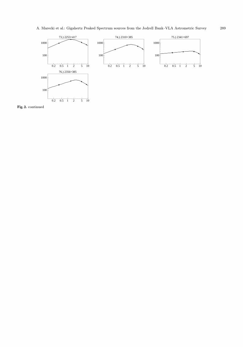
A. Marecki et al.: Gigahertz Peaked Spectrum sources from the Jodrell Bank–VLA Astrometric Survey 289

0.2 0.5 1 2 5 10

100

1000

76.) 2356+385

0.2 0.5 1 2 5 10

100

1000

73.) 2253+417

0.2 0.5 1 2 5 10

100

1000

74.) 2310+385

0.2 0.5 1 2 5 10

100

1000

75.) 2341+697

Fig. 2. continued