BANK OF GREECE

Economic Analysis and Research Department – Special Studies Division

21, Ε. Venizelos Avenue

GR-102 50 Athens

Τel: +30210-320 3610

Fax: +30210-320 2432

www.bankofgreece.gr

Printed in Athens, Greece

at the Bank of Greece Printing Works.

All rights reserved. Reproduction for educational and

non-commercial purposes is permitted provided that the source is acknowledged.

ISSN 1109-6691

WHAT ARE THE INTERNATIONAL CHANNELS THROUGH

WHICH A US POLICY SHOCK IS TRANSMITTED TO THE

WORLD ECONOMIES? EVIDENCE FROM A TIME VARYING

FAVAR.

Anastasios Evgenidis

University of Patras

Costas Siriopoulos

Zayed University

Abstract

In this paper, we examine the international transmission of US monetary policy

shocks across euro area and Asian countries by using a FAVAR model. We first

examine all possible channels through which a policy shock is transmitted to each

country. In general the transmission of the shock hides considerable heterogeneity

across the countries. We find that the trade balance is important in explaining GDP

spillover effects in the case of Singapore. Wealth effects along with the world interest

rate channel explain the negative propagation of the US shock to the GDP of Hong

Kong, the Philippines and Singapore. The exchange rate channel can explain the

positive spillover effects on GDP in Korea and Japan. For the euro area, an

endogenous response of the euro area monetary authority is observed. The wealth

effect through the role of effective exchange rates seems adequate to describe the

transmission of the shock to European countries. For Germany and Italy the decline in

lending and spending reveal the importance of the balance sheet channel in the shock

transmission. Second, we investigate to what extent the transmission mechanism has

changed over time. For the 2007 financial crisis, our results indicate that the majority

of the countries in both regions witness an increase in the size of the shock to real

activity, inflation and credit variables in the post crisis period.

JEL classification: C38, E52, F41

Keywords: Monetary Policy, International Transmission Mechanism, FAVAR,

Bayesian Statistics, Time Varying Parameters

Acknowledgements: The authors would like to thank Heather Gibson for insightful

comments and suggestions as well as the participants at the seminar series of the Bank

of Greece for helpful comments on an earlier version of the paper. Anastasios

Evgenidis also acknowledges financial support from the Bank of Greece for carrying

out this research. The views expressed do not necessarily reflect those of the Bank of

Greece.

Correspondence:

Anastasios Evgenidis

University of Patras

Department of Business Administration

Email: anevg@upatras.gr

3

1. Introduction

The FED has often followed an expansionary policy in order to dampen the

negative effects from a decline in asset prices and provide liquidity until the stock

market recovers. Examples are its intervention in 1998 after the Asian crisis or in

2001 after the dot.com bubble. In the latter case, policymakers lowered rates eleven

times in order to fight recession. However, the recent financial crisis was like nothing

FED has faced since the 1930s. In late 2008, it cut the federal fund rate (FFR) to

nearly zero levels, where it has remained until now. Despite the fact that policymakers

reduced interest rates to historical lows, credit standards tightened and the cost of

credit increased (Krugman, 2008). Since the FED was unable to cut its short-term rate

below zero, it embarked on three rounds of quantitative easing.

In a recent statement, the FED announced that, at some time in the future, the

FFR should return to more normal levels. This will be the first rate increase since

2006 when Bernanke raised rates four times to cool housing markets. Thus it is of

great interest to explore the propagation of a possible US contractionary policy shock

for the first time after the onset of the recent financial crisis. In addition, in a world

economy which has experienced increased global integration in terms of both trade

and financial transactions, such US policy rate shocks will not only affect the US

itself but will spillover to other countries as well. Thus some natural questions to ask

here are: First, how exactly are developed and developing countries affected by an

external US contractionary policy shock? Second, to what extent has the international

transmission mechanism changed with the global financial crisis?

To shed light on these issues we look at all the possible the channels through

which a US policy shock is propagated both in the US and to foreign countries. We

use a time varying factor augmented VAR (FAVAR) model estimated using Bayesian

techniques. The main results we obtain are as follows: All major channels and sub-

channels (trade, wealth effects, expectations, Tobin’s q and credit channels) seem to

be important in the domestic transmission of a contractionary US policy shock. As

concerns the transmission channels to East Asia, they differ according to each

country. First, a US contractionary policy shock results in a GDP decline for all

countries except Korea and Japan. For all East Asian countries except Singapore and

Japan (to a lesser extent), the trade balance does not appear to play any role in the

transmission of the US policy shock. Wealth effects along with the world interest rate

4

channel explain the negative GDP spillover effects found in Hong Kong and

Philippines. By contrast, these channels do not seem to work well for countries

affected positively by the US shock, i.e. Japan and Korea. In these two countries, we

find that the exchange rate channel in effective terms contributes to GDP growth. We

also find that in response to rising output, the central banks of Korea and Japan

respond endogenously by increasing their rates.

Regarding euro area countries, we find that the expenditure switching effect,

through the role of the trade balance, is only consistent with the dynamics in Spain.

The positive effect on the GDP of euro area countries is mainly driven by wealth

effects through the exchange rate. Policy endogeneity holds for all countries in this

region. In addition, we document that for Germany and Italy a tightening US policy

leads to a significant decline in asset prices, lending and spending which highlights

the role of the balance sheet channel in these two countries.

Next, we report if there is evidence of a changing transmission mechanism

through time. We find that the responses of foreign macroeconomic variables to a US

monetary policy shock have changed dramatically over the whole sample. In

particular, the impact of the US policy shock on GDP growth decreased in all euro

area and most East Asian countries during the financial globalization period compared

to the pre globalization period. This can be justified by the decline in the role of US

with the emergence of other large developing economies. For the more recent period,

we find that the impact on GDP has increased almost everywhere during the financial

crisis. The strong impact of US monetary tightening on other economies suggests that

foreign central banks should follow a credible monetary policy in response to the US

shock in order to stabilize output.

The paper is organized as follows. Section 2 presents a description of the

transmission channels together with the relevant literature. Section 3 presents the

FAVAR model in the international context. It also explains the identification and

estimation of the model and, finally, the dataset used in our analysis. Sections 4 and 5

present the results. Section 4 provides a rich discussion of all the possible

transmission channels and sub-channels of the US policy shock to both the US and

non US economies. Section 5 describes how international monetary policy

transmission has changed as a result of financial globalization and the recent subprime

5

crisis. Finally section 6 summarizes the results. The Appendices provide details on the

estimation procedure.

2. Description of transmission channels and related literature

The transmission of a monetary policy shock operates via four major channels

namely investment, consumption, credit and international trade. These channels are

further separated into many sub-channels. For example, the transmission of the shock

via investment may occur through the interest rate channel and Tobin’s q.

Transmission through consumption mainly reflects wealth effects in the sense that a

tightening monetary policy reduces the demand for assets, thereby causing their prices

to fall and reducing agents’ total wealth. Credit channels which arise from the

presence of asymmetric information in the credit markets can be further divided into

the traditional bank lending channel and the balance sheet channel. The latter is the

channel in which we focus on this study. Boivin et al. (2010) provide further details

on how these three channels work in the domestic context.

In the international context, the transmission of a monetary policy shock might

be well described by the traditional Mundell-Fleming-Dornbusch model (MFD).

Under MFD, two important transmission mechanisms may exist. The first is the

income absorption effect, which captures the change in foreign demand for domestic

products due to changes in foreign economic activity. The second is called the

expenditure switching effect and it captures the change in the domestic trade balance

as a consequence of exchange rate movements. These two mechanisms move the

trade balance in opposite directions. Thus, the final effect on output (both domestic

and total) is ambiguous. A full exposition of the MFD model is provided by Obstfeld

and Rogoff (1996). The following schematic depicts how exactly the MFD model

works under these two different mechanisms.

id↑ → E↑→TBd↓ →TBf ↑ →Yf↑

or

id↑→Incomed↓→IMd↓→TBd↑→TBf↓→Yf↓

6

Under the expenditure switching effect, a monetary tightening (id↑) results in

real exchange rate appreciation (E↑) which causes the trade balance (TBd↓) to

deteriorate. This leads to an improvement of the foreign trade balance (TBf ↑) and

finally to a rise in the foreign output.

However a decrease in domestic income (incomed↓) following a

contractionary monetary policy decreases domestic import demand (IMd↓), which

may improve the trade balance. As a result the foreign trade balance deteriorates and

foreign output falls. This is the income absorption effect.

The ambiguous outcome of the transmission mechanism under MFD model

has been modified by the development of a new framework. The intertemporal model

of Svensson and Van Wijnbergen (1989) and Obstfeld and Rogoff (1995) works as

follows.

ius↑→iw↑→Cus ,Ius and Cf ,If↓ →YusandYf↓andIMus, EXus / IMf, EXf↓

A US monetary tightening (ius) will spread internationally since the US is a

large open economy and its monetary policy affects the world’s economies.

Therefore, the rise in the US short-term rate causes the world real interest rate (iw) to

rise since world financial markets are highly integrated. Additionally, the rise in the

domestic interest rate decreases the demand for current consumption (Cus) and also

current investment (Ius). In the same way, the increase in the world real rate reduces

consumption and investment in the foreign country (Cf, If). Consumption and

investment and therefore output in both the US and non US countries may decrease

since real interest rates rise in both US and the non-US countries. In this case both

exports and imports of both the US and non-US economies decline (IMus, EXus/ IMf,

EXf↓).

There is also the possibility that some modified MFD models (some versions

of which are also present in some intertemporal models) might explain the

transmission mechanism. The following schematic depicts how exactly the wealth

effect works.

ius↑ → eus↑/ef ↓ → πf ↑ → total wealthf ↓ → Cf ↓ → Yf↓

Accordingly, following a US monetary tightening (ius↑), the dollar

appreciates/foreign currency depreciates and this raises foreign prices. The increase in

7

inflation leads to a decrease in agents’ total wealth which reduces consumption and

total output.

The balance sheet is another channel which may work in the international

context assuming that foreign policy endogeneity holds. The case of an endogenous

response of foreign banks to an external monetary policy has been studied by Grilli

and Roubini (1995) and Lubik and Schorfheide (2005). According to this mechanism,

in response to a contractionary monetary policy of a large open economy, domestic

inflation and output decline, the dollar appreciates and the final effect is an increase in

foreign output (Yf ↑) under the expenditure switching effect. In order to moderate the

increase in output, the foreign monetary authorities might respond endogenously to

these developments by increasing their short-term rates. The rise in foreign short-term

rates may lead to a decline in equity prices (Peq,f↓) which lowers the net worth of

firms through Tobin’s q. With less cash flow, the firm has fewer internal funds and

must raise funds externally. Since external funding is subject to asymmetric

information, leading to adverse selection (AS) and moral hazard (MH), the fall in

firms’ net worth is important since it lowers the collateral they can post. This leads to

a fall in investment and total output. The schematic is depicted below:

ius ↑→Yf ↑ and so if↑

thus:

if ↑→Peq,f↓ (Tobin’s q) → net worth f ↓ →AS,f / MH,f↑ →Yf↓

Our paper contributes to the literature in a number of ways. First, we examine

how a US policy shock is transmitted in practice to specific developed and developing

countries. For this reason, we consider two separate world regions. We choose major

European countries to examine the effect in developed countries and East Asian

economies to examine the effect on developing countries. We use a FAVAR model,

which incorporates a large set of macroeconomic and financial variables representing

various dimensions of these economies. Other studies which use information from a

large set of macroeconomic variables to examine the international propagation of

shocks include Boivin and Giannoni (2008), Mumtaz and Surico (2009) and

Eickmeier et al. (2011). These papers, however, differ significantly from our study.

The first paper uses a FAVAR model to study exactly the opposite effect, i.e. the

impact of international events on the US economy. The second focuses on the effect

8

of various international shocks on the UK economy while the third focuses on the

effect of a US financial shock in selected foreign economies. Kim (2001), and Neri

and Nobili (2006) examine the propagation of a US policy shock to the euro area but

they use VAR models which rarely employ more than five to seven variables.

Arguably, our approach is more realistic since central banks monitor and respond to

much larger information set than typically assumed in VAR models. As concerns East

Asia, the only relevant studies are those of Miniane and Rogers (2007) and Kim and

Yang (2012). Again, both papers use VAR models and they only explore the effect of

a US monetary policy shock on interest rates and exchange rates.

The second contribution is that we employ a model which allows us to

estimate time-varying impulse responses for a wide variety of macroeconomic

variables in EU and Asian countries. All previous studies except Eickmeier et al.

(2011), who examine a financial shock, assume that the parameters remain constant

over time. The most relevant study in the spirit of our paper is that of Kazi et al.

(2013). The two analyses however differ along a number of dimensions, including the

FAVAR estimation and the countries analyzed in the empirical application. Most

importantly, their analysis provides a very limited picture of how the international

transmission channels work based only on interest rates, stock prices and exchange

rates. This leads to the third contribution. In order to investigate the richness of the

international propagation of US policy shocks we examine their effects on a large

number of variables that may be of interest other than just interest rates and exchange

rates. Therefore we are able to provide a detailed analysis for each country of all the

possible transmission channels (and sub-channels) which have not been covered

previously.

Fourth, our paper is related to the growing literature studying changes in the

monetary transmission mechanism over the years (e.g. Mumtaz et al., 2011; Boivin et

al., 2008 and 2010;Korobilis, 2013). However, none of these studies have examined

the changing US transmission mechanism internationally. To the authors’ knowledge,

only the recent studies of Ilzetski and Jin (2013) and Fukuda et al. (2013) deal with

the changing dynamics of the international transmission of a US shock. These papers

mainly focus on the changing spillover effects in the pre financial crisis period. They

both conclude that there is a significant change in the international propagation of US

policy shocks in the later, more globalized, decades. In respect to these studies, we

9

examine how monetary transmission has changed as a result of the deepening of

financial globalization. In doing so, we extend the relevant literature in the following

ways. First, while all previous studies focused on the changing international

transmission by splitting the sample, our time varying FAVAR permits us to examine

what was happening at different points in time. In this way, we avoid the estimation

over different subsamples. The superiority of this technique is noted by Boivin and

Giannoni (2006). They point out that the evolution of monetary transmission is quite

complex to be captured solely by splitting the sample. Second, we investigate possible

changes in the international propagation of US monetary policy shocks between the

pre and post crisis period. Third, previous papers provide results for the changing

dynamics only for the core foreign variables such as output, exchange rates and

interest rates. In contrast, we look at the changing transmission of the shock to

measures of real activity other than GDP and measures of trade activity other than

nominal and effective exchange rates. We also consider the changing transmission of

the policy shock to stock prices, credit variables and monetary aggregates.

3. Econometric framework

The information about the US and the world economies is summarized in the

following vector of K latent factors'

,w us

t t tf f f , where w denotes the foreign

economies. We also consider the US short-term interest rate Rt as the only observable

factor, thus the dynamics of the unobserved factors together with the observable

factor can be described using a VAR (p) model:

1 1 ...t t t pt t p tF F F u (1)

where '

,t t tF f R with tf a (Kx1) vector of latent factors, Bit is a (KxK) coefficient

matrix and tu (0, )t ,where t is a full (KxK) covariance matrix.

The unobserved factors are extracted from a large panel of N macroeconomic

variables which provide a representation of the US and foreign economies. The

original observed series Xt of (Nx1) dimensions are linked to the factors and the

monetary policy tool by the observation equation:

10

f R

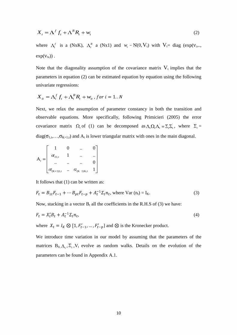
t t t tX f R w (2)

where f

t is a (NxK), R

t a (Nx1) and (0,tw Vt) with Vt= diag (exp(ν1t..,

exp(νNt)) .

Note that the diagonality assumption of the covariance matrix Vt implies that the

parameters in equation (2) can be estimated equation by equation using the following

univariate regressions:

f R

it i t i t itX f R w ,

Next, we relax the assumption of parameter constancy in both the transition and

observable equations. More specifically, following Primicieri (2005) the error

covariance matrix t of (1) can be decomposed as ' '

t t t t t, where t =

diag(σ1,t,…,σΚ+1,t) and At is lower triangular matrix with ones in the main diagonal.

21,t

(K 1)1,t (K 1)K,t

1 0 .. 0

1 .. ..

.. .. .. 0

.. 1

t

It follows that (1) can be written as:

, where Var (nt) = IK. (3)

Now, stacking in a vector Bt all the coefficients in the R.H.S of (3) we have:

(4)

where ] and is the Kronecker product.

We introduce time variation in our model by assuming that the parameters of the

matrices Bit, t, t ,Vt evolve as random walks. Details on the evolution of the

parameters can be found in Appendix A.1.

11

3.1 Identification method

We estimate the factors and the associated loadings from equation (2) by

standard principal components. We first follow Bernanke et al. (2005) by restricting

the factors according to' /f f T I , where T is the number of time periods. Then,

according to Mumtaz and Surico (2009), we identify the US and the international

factors as follows. The K1 international factors are identified through the upper N x

K1 block of the matrix f which is assumed to be a block diagonal matrix. The

dynamics of the US factors are captured by K2 factors. These factors are identified

through the bottom N x K2 block of f which is a full matrix. In our model, we

include four international factors to capture the effects of real activity, inflation, trade

variables and asset prices including monetary aggregates. We also include four

domestic factors to capture the dynamics of the US economy. When we experimented

with three and five factors (as Bernanke at al. (2005) did)we find no significant

changes in our impulse responses.

Second, we follow Bernanke et al. (2005) in order to identify the monetary

policy shock in the VAR equation (1). We identify the US monetary policy shock as

the only shock that does not affect contemporaneously the other domestic factors in

the system. This implies that the underlying US series do not respond

contemporaneously to policy innovations. Since a subset of series mainly financial

variables are likely to respond to monetary policy innovations within the quarter, we

need to remove the contemporaneous relationship between the federal fund rate (FFR)

and the financial variables. To achieve this, we proceed as follows. We first divide

our data set into slow moving and fast moving variables depending on how fast they

respond to the US policy shock. Then we extract K2+1 principal components from the

US variables in Xt to obtain consistent estimates of Ct=( US

tf , tR ). Notice that

Bernanke et al. (2005) do not impose the constraint that FFRis one of the common

components, so if FFR is really a common component it should be captured by the

principal components. Third, we estimate slow moving factors ,US slow

tf as the principal

components of the US slow moving variables. Fourth, we estimate the following

regression:

,

1 2ˆ US slow

t t t tC b f b R (5)

12

from which we obtain ,

1ˆ US slow

t tC b f . Then the identification of the domestic

monetary policy shock is achieved by recursively ordering: w

tf ,,

1ˆ US slow

t tC b f , tR

with tR last in the VAR equation. This ordering imposes the assumption that both

international and domestic latent factors do not respond to monetary policy

innovations within the quarter.

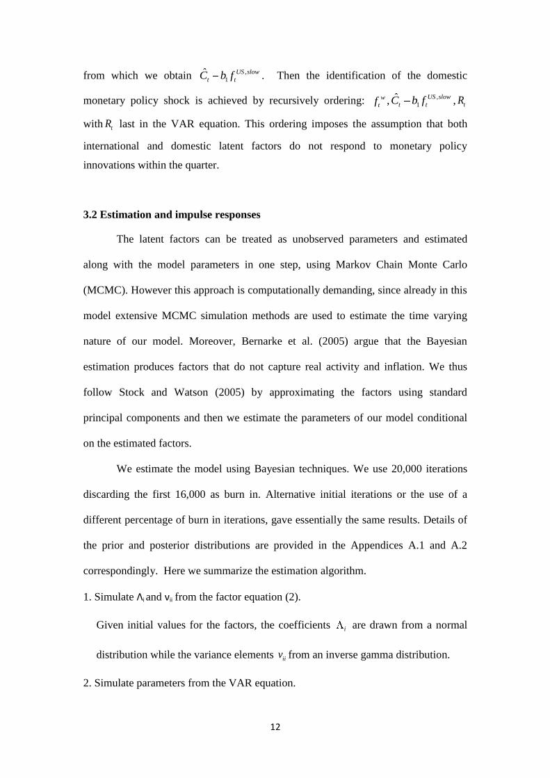
3.2 Estimation and impulse responses

The latent factors can be treated as unobserved parameters and estimated

along with the model parameters in one step, using Markov Chain Monte Carlo

(MCMC). However this approach is computationally demanding, since already in this

model extensive MCMC simulation methods are used to estimate the time varying

nature of our model. Moreover, Bernarke et al. (2005) argue that the Bayesian

estimation produces factors that do not capture real activity and inflation. We thus

follow Stock and Watson (2005) by approximating the factors using standard

principal components and then we estimate the parameters of our model conditional

on the estimated factors.

We estimate the model using Bayesian techniques. We use 20,000 iterations

discarding the first 16,000 as burn in. Alternative initial iterations or the use of a

different percentage of burn in iterations, gave essentially the same results. Details of

the prior and posterior distributions are provided in the Appendices A.1 and A.2

correspondingly. Here we summarize the estimation algorithm.

1. Simulate Λi and νii from the factor equation (2).

Given initial values for the factors, the coefficients i are drawn from a normal

distribution while the variance elements iiv from an inverse gamma distribution.

2. Simulate parameters from the VAR equation.

13

Given initial estimates for the factors:

We first draw t from a conditionally normal density using a standard state

space filter and smoother (Carter and Kohn, 1994). Next, conditional on t we

draw the covariance matrix Q from an inverse Wishart distribution.

Given t we draw coefficient states ,i t

using the methods described in the

previous step. We then draw the hyperparameter S conditional on estimates of

At elements from an inverse Wishart.

Last we draw volatility states log t by using Kalman filter methods

introduced in Kim, Shepard and Chib (1998) for nonlinear and non-Gaussian

state space forms. Again, the corresponding covariance matrix W is drawn

easily from an inverse Wishart posterior.

3. Go to step 1.

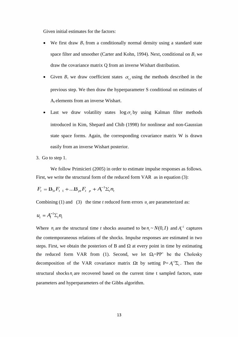
We follow Primicieri (2005) in order to estimate impulse responses as follows.

First, we write the structural form of the reduced form VAR as in equation (3):

1

1 1 ...t t t pt t p t t tF F F A n

Combining (1) and (3) the time t reduced form errors tu are parameterized as:

1

t t t tu A n

Where tn are the structural time t shocks assumed to be tn ~ (0, )N I and 1

tA captures

the contemporaneous relations of the shocks. Impulse responses are estimated in two

steps. First, we obtain the posteriors of B and Ω at every point in time by estimating

the reduced form VAR from (1). Second, we let Ωt=PP’ be the Cholesky

decomposition of the VAR covariance matrix Ωt by setting P= 1

t tA . Then the

structural shocks tn are recovered based on the current time t sampled factors, state

parameters and hyperparameters of the Gibbs algorithm.

14

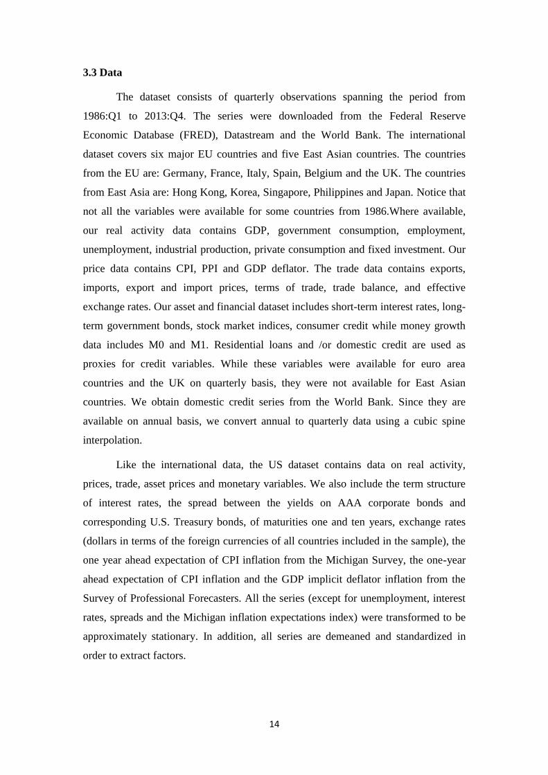
3.3 Data

The dataset consists of quarterly observations spanning the period from

1986:Q1 to 2013:Q4. The series were downloaded from the Federal Reserve

Economic Database (FRED), Datastream and the World Bank. The international

dataset covers six major EU countries and five East Asian countries. The countries

from the EU are: Germany, France, Italy, Spain, Belgium and the UK. The countries

from East Asia are: Hong Kong, Korea, Singapore, Philippines and Japan. Notice that

not all the variables were available for some countries from 1986.Where available,

our real activity data contains GDP, government consumption, employment,

unemployment, industrial production, private consumption and fixed investment. Our

price data contains CPI, PPI and GDP deflator. The trade data contains exports,

imports, export and import prices, terms of trade, trade balance, and effective

exchange rates. Our asset and financial dataset includes short-term interest rates, long-

term government bonds, stock market indices, consumer credit while money growth

data includes M0 and M1. Residential loans and /or domestic credit are used as

proxies for credit variables. While these variables were available for euro area

countries and the UK on quarterly basis, they were not available for East Asian

countries. We obtain domestic credit series from the World Bank. Since they are

available on annual basis, we convert annual to quarterly data using a cubic spine

interpolation.

Like the international data, the US dataset contains data on real activity,

prices, trade, asset prices and monetary variables. We also include the term structure

of interest rates, the spread between the yields on AAA corporate bonds and

corresponding U.S. Treasury bonds, of maturities one and ten years, exchange rates

(dollars in terms of the foreign currencies of all countries included in the sample), the

one year ahead expectation of CPI inflation from the Michigan Survey, the one-year

ahead expectation of CPI inflation and the GDP implicit deflator inflation from the

Survey of Professional Forecasters. All the series (except for unemployment, interest

rates, spreads and the Michigan inflation expectations index) were transformed to be

approximately stationary. In addition, all series are demeaned and standardized in

order to extract factors.

15

4. The channels of monetary transmission in the US and the world

economies

4.1 Cross country differences

The transmission of the US policy shock internationally hides considerable

heterogeneity across the countries. Looking at Figures 2 and 5 we observe that a

surprise increase in the US short-term rate is positively transmitted to GDP (or

industrial production)in all EU countries and some East Asian countries and

negatively transmitted in Hong Kong, the Philippines and Singapore. Moreover, the

magnitude of the effect also varies across the countries. For example, the GDP of the

developed countries (EU and Japan) is more affected by the US policy shock

compared to the developing countries on East Asia. The international transmission

hides a significant degree of heterogeneity not only for the effect on GDP but also for

many other important macroeconomic indicators of the foreign economies. The effect

of the US policy shock on inflation for example (Fig. 2 and 5) may be positive and

significant (Philippines, Korea, Japan, Germany and Italy), or negative and significant

(Singapore) or even insignificant (Hong Kong, UK, Spain). As concerns interest rates,

Hong Kong, Korea and the UK see a much larger increase in their short term rates

than the other countries (Fig. 4 and 7). Similarly, the movements in foreign currencies

with respect to other major currencies differ in the sign and magnitude of the effect. In

particular, the real effective exchange rates (REER) of Hong Kong and Japan

depreciate over time whereas all the other Asian and EU currencies appreciate on

impact in response to the US contractionary policy shock (Fig. 3 and 6). In the

following sub sections we provide a detailed analysis of the transmission of monetary

policy disturbances in US, East Asia and EU.

4.2 Detailed transmission mechanism of the U.S. policy shock domestically

Before examining the effects abroad, we examine the domestic channels

through which monetary policy exerts its influence on the US economy (see Fig. 1).

The impulse responses in general act as expected under a contractionary policy shock.

Output decreases gradually, prices eventually go down and monetary aggregates also

decline. Consistent with the relevant literature (see Bernanke et al., 2005 and

Korobilis, 2013), the negative correlation between nominal interest rates and inflation

suggest that the FAVAR methodology properly manages to deal with the price puzzle

16

observed in VAR models. Next, we also notice a negative correlation between interest

rates and the money stock. Thus, the liquidity effect observed in the VAR literature is

absent. Last, an apparent problem in open economy studies is the exchange rate and

forward discount puzzle. Under Dornbusch’s overshooting hypothesis, an increase in

interest rates should cause the nominal exchange rate to appreciate instantaneously

and then depreciate according to uncovered interest parity (UIP). Our results show

that the exchange rate puzzle is not present in the FAVAR model. Figure 1 shows

exchange rates defined as the national currency of each member country per US

dollar, so an increase in the exchange rate shows appreciation of dollar. One notices

that the contractionary policy shock leads to an initial depreciation for all foreign

exchange rates. After the depreciation there is a gradual appreciation in the majority

of the currencies which is fully consistent with Dornbusch overshooting hypothesis.

These initial results suggest that the exchange rate channel does play a crucial role in

the monetary transmission mechanism. We will verify the importance of this channel

by looking at the REER in the next sections.

To further infer details about the transmission channels in the US we also look

at the response of other variables. We begin with the trade balance. There is a slight

improvement in the trade balance in the short term which dies out in the medium and

long term. Thus the income absorption effect in the short run is consistent with the

dynamics. Second, the rise in the short-term rate reduces consumption and investment

via wealth effects and lowers equity prices via Tobin’s q. Therefore, both channels are

sensible ways to describe the effects of a tightening monetary policy in the economy.

Third, we explore whether the expectation channel plays a significant role in the

transmission mechanism. The results suggest that eventually there is a significant

reduction in expected inflation as indicated by the index of consumer expectations,

which implies that the expectations channel does matter in the transmission of a

policy shock. Last, we investigate if contractionary monetary policy can exert an

influence on the US economy by affecting the balance sheets of consumers and firms.

To measure the impact of this channel we report the responses of two variables. These

are consumer credit and the spread between the yield on AAA corporate bond and the

three month T Bill. The latter can be seen as a proxy for the external finance

premium. In accordance with theory, there is a reduction in the response of credit

which means that consumers’ access to the credit has reduced. There is also an

17

increase in the size of the external finance premium which means that lenders are less

willing to make loans.

4.3 Detailed transmission mechanism of the U.S policy shock to East Asia

The effect of a US policy shock on the East Asian countries can be seen in

Figures 2, 3 and 4. Figure 2shows impulse responses of real activity and inflation

measures, Figure 3 shows impulse responses of trade activity variables while Figure

4depicts asset price variables. A US shock results in a decline in GDP in all countries

except Korea and Japan (Fig.2). The response of unemployment in Hong Kong and

the Philippines is counter to theory since we would expect a rise in the unemployment

rate following a decline in output. To further investigate the evolution of monetary

policy, we examine which of the transmission channels might have been involved in

international transmission of the shock.

We begin by analyzing the role of the trade balance channel. Under MFD, the

final effect on the foreign output is ambiguous. On the one hand, the higher US policy

rate results in dollar appreciation which makes domestic goods in the US more

expensive than foreign goods. This leads to a deterioration of the trade balance, an

improvement in the foreign trade balance and finally an increase in foreign output.

However, a rise in interest rates may have exactly the opposite effect on foreign

output. Following a contractionary policy, domestic income is reduced. Thus the

demand for the domestic imports is also reduced, leading to an improvement in the

US trade balance through the expenditure switching effect. Our results indicate that a

monetary tightening leads to a slight initial increase in the trade balance (Fig. 3) for

Hong Kong and Philippines which very soon dies out and can thus be considered

negligible. The same holds for Japan. The income absorption effect is consistent with

the results for Singapore since there is a significant worsening of its trade balance

which justifies the fall in output. Last, although the trade balance does not explain the

rise in output in Korea, it is a significant transmission mechanism since there is a clear

reduction in its response. In sum, the trade balance channel cannot satisfactorily

describe the international transmission mechanism to East Asian countries with the

exception of Singapore.

18

Second, we explore the role of the international wealth effect channel in the

transmission mechanism. According to this channel, a US monetary tightening results

in the depreciation of the foreign currency leading to an increase in foreign inflation.

Then- in line with the Pigou effect -foreign output decreases due to the decrease in

real balances of wealth. Figure 2shows that this channel might operational for Hong

Kong and the Philippines since there are significant increases in inflation which may

cause GDP to fall.

Another channel through which shocks are transmitted internationally is

through the world interest rate (intertemporal model of Obstfeld and Rogoff, 1995).

According to this, the final effect of the US monetary tightening to the foreign

economies will be a reduction in consumption, investment and therefore output.

Imports and exports will also decrease since residents in both the US and the world

economies reduce the demand for goods and services in the US and non US countries.

To assess the relevance of the world markets in the transmission of the monetary

shocks to East Asia we study the responses of the aforementioned variables.

Consistent with the theory, consumption and investment (Fig. 2) fall in Hong Kong

while the response of investment in Singapore does not work well. To further

recognize the importance of this channel for these countries we report the responses

of exports and imports (Fig. 3). The final effect of the US shock is a substantial

decrease in both imports and exports for Hong Kong, Singapore and Philippines. This

makes the world interest rate channel a significant channel for these three countries.

Overall it can be argued that the combination of the wealth effect channel

along with the world interest rate and (to a lesser extent)the trade balance are quite

helpful in explaining the negative GDP responses in Hong Kong, the Philippines, and

Singapore. However, none of these channels manage to describe adequately the

spillover effects to Korea and Japan. The positive effects on consumption, investment

and finally output in both countries (Fig. 2) might be a result of the foreign currency

depreciation with respect to other currencies of trade partners. Therefore we examine

if the exchange rate channel may be operating in these countries. Indeed, as Figure 3

depicts, the REER for Japan and Korea depreciate and as a result exports in both

countries increase which means that this channel works well for these countries.

We also examine whether central banks appear to respond to the US

tightening. Japan and Korea increase their short-term rates in order to mitigate the

19

boost to inflation and economic activity observed after the US policy shock (see Grilli

and Roubini, 1995).To examine this possibility we look at the responses of short-term

rates and monetary aggregates for these countries. Following a rise in output and

inflation (see Fig. 2), we notice that there is a significant rise in the short-term rates

for Japan and Korea (Fig. 4) which is consistent with our hypothesis. In addition,

there is also a significant reduction in the monetary aggregates (M1) for both

countries. Notice also that this channel does not contribute to the transmission of

external shocks to the rest of East Asia countries since the responses in short rates and

monetary measures either have opposite signs or move in line with theory but are

insignificant.

4.4 Detailed transmission mechanism of a policy shock to the EU

Figures 5-7 show the impulse responses of the largest EU economies to a US

monetary policy shock. In all cases, a monetary tightening leads to gradual increases

in output (either real GDP or industrial production, Fig. 5). Notice that the rise in

foreign output produces a significant reduction in unemployment for all the countries

except Germany. In line with the analysis in the previous section we discuss the

transmission channels that may generate the positive spillover effects for the EU.

First we can exclude the intertemporal model since, according to this theory,

we would expect a significant reduction in GDP in EU countries as a result of the US

shock. Next, in order to verify if the increase in the foreign output is consistent with

the expenditure switching effect, we examine the significance of the trade balance

channel in the international transmission. If this channel works then a significant

increase should be found in the trade balance in order to justify the increase in output.

Our results indicate that this channel does not explain the positive spillover effects

observed on GDP since we would expect a rise in trade balance in euro countries. An

improvement in the trade balance is only observed for Spain (Fig. 6).Next, we look at

the role of exchange rates in the transmission of the shock. Judging from the bilateral

exchange rate responses (Fig. 1), the depreciation of both currencies (euro and pound)

against the dollar may provide a good explanation of the rise observed in foreign

output in EU countries. However this is not consistent with the response of exports in

20

EU countries and the UK; exports fall which is not consistent with the currency

depreciation.

To consider the role of exchange rates in the transmission mechanism we look

at the REERs since they provide more accurate measures of price competiveness. The

REER is the nominal effective exchange rate divided by the price deflator index of

each country. Figure 6 shows that in contrast with bilateral exchange rates, there are

significant appreciations in all REERs. This is in line with Edwards (1995). The

appreciation in the REERs confirms the deterioration in export performance for all

European countries as a result of the shock. The appreciation of the effective

exchange rate, combined with the decrease in inflation (Fig. 5) for all EU countries,

explains the increase in consumption (Fig. 5) and therefore GDP through the wealth

effects. We conclude that that the wealth effects through the exchange rate channel do

play a significant role in the transmission of the US shocks to the EU.

We also examine if foreign policy endogeneity is present in the EU countries.

Indeed, we find that in response to rises in output, short-term rates (Fig. 7)increase in

all countries except Germany. Moreover, we notice a significant reduction in the

monetary aggregates (Fig. 7), which further confirms the hypothesis that short-term

interest rates in the euro area respond endogenously to a US monetary contraction.

Consistent with the hypothesis of policy endogeneity in the EU, there is

another channel that might work which is the balance sheet channel. If foreign central

banks follow a contractionary policy- as a result of the US policy shift –this leads to a

decline in asset prices which lowers the net worth of firms. Lower net worth means

less collateral available and increasing adverse selection and moral hazard problems.

As a result, there will be a decline in lending, spending and aggregate demand. This

appears to closely follow the case of Germany and Italy. First, notice that equity

prices decline in response to a rise in the short-term rates (Fig. 7). Then there is a

clear reduction in the responses of consumer credit or/and bank lending which

suggests that the consumers’ access to credit is diminished. Obviously, this channel

also offers an explanation of why the response of consumption in Germany is

negative. Notice that there is an ambiguous effect for the responses in UK since the

resulting negative asset price effects in the UK are not sufficient to lead consumer

21

credit to lower levels. For the rest of the countries this channel does not seem to

matter for the international transmission.1

4.5 Policy Implications

The financial crisis that started in 2007 has had different effects across the

world economies. While before the 2007 crisis macro-financial linkages had ensured a

more homogeneous transmission of an exogenous shock to other countries, since 2008

the interconnections between market segments have largely broken, also across

borders. Thus the monetary transmission mechanism has operated in a context of

heterogeneity in the global economies which means that policymakers in both the

euro area and East Asian countries plan the performance of the monetary policy

stance in a different way.

The previous findings are related to policymaking in both a direct and an

indirect way. The description of the transmission channels through which the US

policy shock is transmitted internationally is the indirect way. More specifically, the

insignificant role of the trade balance, the importance of the wealth effects for both

regions, the strong impact of the world real interest rate channel and the exchange rate

channel in Asian countries, the considerable role of the balance sheet channel in some

euro area countries, all shed light on the correct theoretical models for international

monetary policy analyses.

In particular, as concerns East Asian countries, monetary policy authorities in

Singapore and Korea should take into account the role of the trade balance when

forecasting the implications of US monetary policy actions on their economies. The

central banks of Hong Kong, Philippines and Singapore should focus their forecasts

on transmission through wealth effects. In addition, the monetary authorities in Hong

Kong, Singapore and the Philippines should attention to the transmission of a US

shock via the world interest rate channel. This is because all these countries witness a

significant reduction in many macroeconomic variables affected by this channel

(consumption, investment, exports and imports).

1 Consistent with the discussion in the previous section, the balance sheet channel might also works for

Japan and Korea since policy endogeneity holds only in these countries. However the examination of

the responses rejects this hypothesis for both countries since equity prices and consumer credit move in

opposite directions.

22

Overall it can be argued that the combination of the wealth effect channel

along with the world interest rate channel and (to a lesser extent) the trade balance are

quite helpful in explaining the negative GDP responses in Hong Kong, Philippines,

and Singapore. However, none of these channels manage to describe adequately the

spillover effects to Korea and Japan. Our results indicate that the only channel

explains the GDP spillover effects in Korea and Japan is the exchange rate channel

which means that policymakers should focus on their currencies when forecasting the

implications of a US monetary tightening..

As with East Asian countries, in all EU countries except Spain, the trade

balance channel cannot adequately describe the transmission of the shock. Moreover,

the significant reduction observed in individual inflation rates as a result of the

appreciation of the effective exchange rates also denotes the important role of the

wealth effects in the transmission of the shock. This suggests the need to focus on

exchange rates and inflation when forecasting the impact of tightening in the US.

Additionally, an extra channel which plays a significant role in the transmission of the

shock in two euro countries, i.e. Germany and Italy, is the balance sheet channel. Our

results indicate that there is a clear reduction in the equity prices and consumer credit

as a result of the US shock. This implies that the role of credit markets in the

transmission of the shock especially in these two large euro area countries should be

seriously considered.

Aside from the indirect effect described above, there is also the direct effect.

The examination of some of the variables of primary interest such as output and

inflation are directly related to the policymaking. For example, in the US, the

monetary tightening leads in a short improvement of its trade balance. Since the US is

a country with trade deficit, it can use contractionary policy to improve its trade

balance. Similarly, a monetary tightening achieves lower inflation. By contrast, a rise

in the policy rate has no significant effects in imports and exports thus a US monetary

contraction is not a desirable policy in this case.

In the international context, the case of an active foreign monetary policy as a

result of the US shock is given by the endogenous responses of two East Asian

countries central banks, i.e. Korea and Japan and the monetary authority in euro area.

In particular, our results indicate that a US contractionary policy leads to a significant

increase in the output of EU countries. This means that in terms of GDP growth, these

23

countries will initially see the US monetary tightening as a desirable policy. However,

over the long term, the foreign central banks of all these countries will strongly

respond by increasing their short-term rates order to cool economy boost and

inflationary pressures from the unexpected US shock. Indeed, the responses of output

for all EU countries and Korea and Japan show that after 12 months the initial

increase in the level of economic activity has faded. This fading is the result of the

endogenous monetary policy response of the foreign central banks.

5. Investigating the changing transmission mechanism of the U.S.

shock

In contrast with the relevant literature which deals with changes in the

transmission mechanism by estimating the FAVAR model over different subsamples

(see Boivin et al., 2009 and Mumtaz et al. 2011), our time varying model permits us

to examine what was happening at different points in time. In addition, as Boivin and

Giannoni (2006) point out, the evolution of the monetary transmission is too complex

to be captured solely by splitting the sample. We determine whether the monetary

transmission mechanism has changed through the years as a result of two important

worldwide phenomena, i.e. a) the globalization of finance and b) the US subprime

crisis. For this reason, we choose in our analysis four representative dates, i.e. 1987,

1999, 2007 and 2013. We choose1987 as it is considered the beginning of global

integration (Kose et al, 2007)and therefore it can be seen as a representative date of a

less integrated period. The date 1999 has been chosen for three reasons. First it gauges

the impacts of the gradual deepening of financial integration (compared with 1987).

Second, it is a benchmark date for euro area countries since it is the year of the

adoption of the common currency, while it is also a time period after the Asian crisis

of 1997. Therefore many significant changes might be observed in the propagation of

US policy shock to most of the countries in the sample. Last, 2007 represents the pre-

crisis period while 2013 is indicative of the post financial crisis period. Our results

focus on the effect after one year and posterior medians of impulse responses on these

four representative dates.

24

5.1 How has the monetary transmission evolved in U.S.?

We begin by analyzing the changing transmission mechanism in the US. Table

1 shows that the effect on real activity variables (except unemployment) is of greater

magnitude during the latest years (2007 and 2013) compared with the earlier years

(1987 and 1999). As an additional comment, one could also note that GDP,

consumption and investment respond more in the pre-crisis period (2007) rather than

in the post-crisis period (2013). In accordance with real activity variables, inflation

responses are also large before the outbreak of the crisis but small and insignificant in

its aftermath. In terms of asset prices and monetary variables, the impact of the policy

shock is strong in most of the variables (with the exception of mid and long-term

rates) at all points in time. The effect is stronger for stock indices, short-term rates and

monetary aggregates in the pre-crisis period compared to post-crisis. In addition,

during the post-globalization period (1999) the impact on all variables (except for the

short-term rate) has increased compared to pre-globalization period.

The estimates of trade activity variables display very similar patterns to those

presented above. In particular, the terms of trade and the REER are stronger in 2007

(compared with 2013) and in 1999 (compared with 1987). The responses of imports

and exports show no signs of change between the pre and post-financial crisis period.

On the contrary, there are important changes in the responses of both variables in the

earlier years. Notice that with greater financial integration (compared with the pre-

globalization period), the spillover effects on both variables become weaker.

Last, we report the results from the nominal exchange rates of dollar against

East Asian currencies, the euro and the British pound. There is a clear evidence of

time variation for all exchange rates. However the magnitude of the effect differs

across the different regions. In particular, both the euro and the pound are affected

more after the financial crisis period, while the opposite holds for Asian currencies. In

addition, all Asian currencies depreciated before the crisis but most of them

appreciated after 2007. The depreciation of the dollar against the Asian currencies in

the post crisis period is consistent with the overshooting hypothesis stating that an

increase in the short-term rate will cause the nominal exchange rate to appreciate

instantaneously (not shown here since we focus on the effect one year after the shock)

and finally depreciates. By contrast, a possible explanation for the consistent dollar

25

appreciation in the years before financial crisis is the fact that the US was considered

as a ‘safe haven’ by investors.

5.2 How has the monetary transmission evolved in the world economies?

We first report the results for each different sector of the economy (sections

5.2.1, 5.2.2 and 5.2.3).Then, in section 5.3 we provide an economic explanation of our

findings.

5.2.1 Time variation in real activity variables

Table 2 depicts the changing transmission mechanism through the foreign real

activity variables. The impact of US policy shocks on GDP between 1987 and 1999

has decreased for almost all countries (except Hong Kong and Philippines). In

general, we find that all real activity variables in most of the non US countries fall in

response to a contractionary US policy shock under global integration.

In the more recent period (pre and post crisis), the magnitude of the effect on

GDP is far smaller than the pre-globalization period. This means that the effect of a

US policy shock on foreign output has diminished through time. Note that, between

2007 and 2013, the pass through of policy shocks to output has increased in all

countries with the exception of Singapore. What is more, during these latest periods,

the transmission mechanism generates not only positive (as in the earlier years, 1987

and 1999) but also negative spillover effects, only in some East Asian countries.

The impulse responses of unemployment are in general statistically

insignificant for the whole period examined. Consistent with the responses in output,

the impact on GDP components such as consumption and investment is larger in 1987

compared to 1999 for all countries. During the crisis, for most of the countries (Japan,

Korea, France, Italy and UK) the effect on consumption and investment has risen

compared with the pre-crisis period.

5.2.2 Time variation in trade and price variables

In terms of trade variables, Table 3 shows that the negative impact on exports

has risen for almost all countries in 2013which is indicative of the worldwide trade

breakdown in the aftermath of the crisis. The only countries which see their exports

26

affected less by the shock are Korea and Singapore. One also notices that in the pre-

crisis period, the responses of export measures are all negative except Germany. This

result confirms Germany’s strong export performance in the pre-crisis period since it

appears that its exports stay unaffected by foreign contractionary policy shocks.

Further, we find that in contrast to the responses in the more recent years (2007 and

2013), there is a positive effect on exports in almost all countries during the earlier

years. Moreover, the impact of a US monetary policy shock is general weaker in the

post globalization period compared to the pre-globalization period.

For the rest of trade variables, the signs and magnitude of import responses are

similar to those of exports at all representative dates. There is also no evidence of

significant time variation in the trade balance in any period. In the case of exchange

rates, there is a distinguishable pattern between the two regions in the latest years. All

Asian currencies show stronger spillover effects - in real effective terms -before the

crisis in comparison with 2013,while all REERs from EU countries how a larger

response during the post crisis period. Evidence of time variation in exchange rates is

also observed between the pre and post globalization periods but there is no clear

pattern of the REER responses between these two periods. Additionally, the negative

signs observed mainly in the REERs of East Asia economies through time, indicate

that a US contractionary policy shock gives these countries the opportunity to increase

their exports since their currency relative to other major currencies depreciate.

Concerning aggregate price variables, the impulse responses of inflation (both

CPI and GDP deflator) show significant time variation between 2007 and 2013. On

average, the response of inflation is large and negative (except for Korea and The

Philippines) during the post crisis period while before 2007 the magnitude of the

effect is smaller and positive in many cases. Similarly, the inflation responses show

signs of change over time between 1987 and 1999, while the responses are mainly

negative and stronger in the pre -globalization period.

5.2.3 Time variation in asset price variables

We analyze the responses of some key asset price variables through time as it

can be seen in Table 4. First, notice that short-term rates respond more to a US policy

shock in the pre globalization period (compared with post globalization period) and in

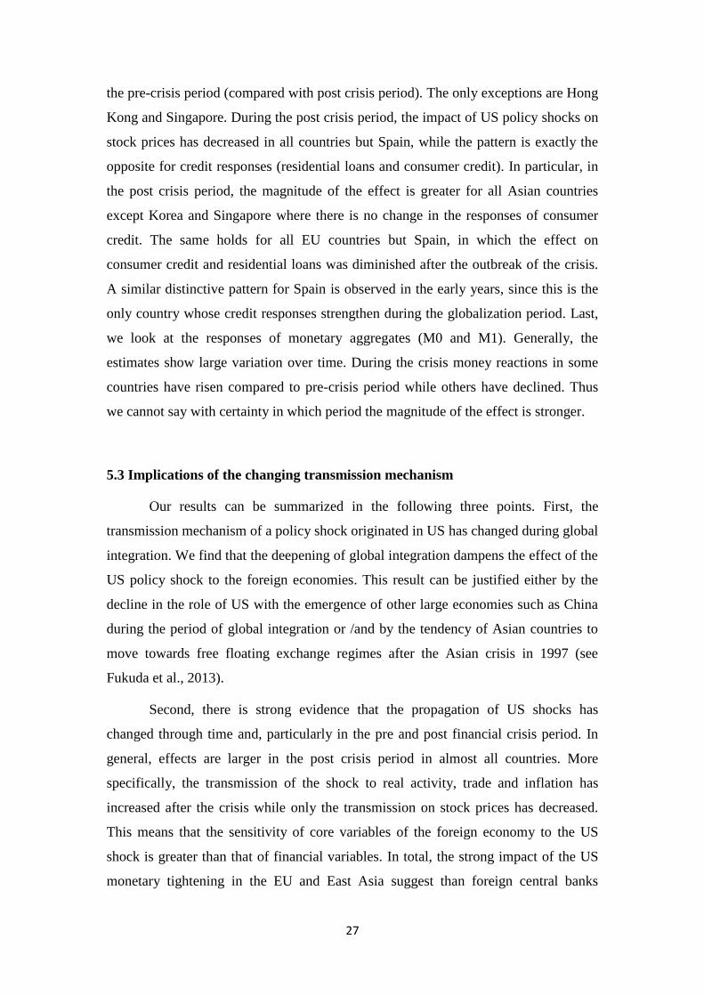
27

the pre-crisis period (compared with post crisis period). The only exceptions are Hong

Kong and Singapore. During the post crisis period, the impact of US policy shocks on

stock prices has decreased in all countries but Spain, while the pattern is exactly the

opposite for credit responses (residential loans and consumer credit). In particular, in

the post crisis period, the magnitude of the effect is greater for all Asian countries

except Korea and Singapore where there is no change in the responses of consumer

credit. The same holds for all EU countries but Spain, in which the effect on

consumer credit and residential loans was diminished after the outbreak of the crisis.

A similar distinctive pattern for Spain is observed in the early years, since this is the

only country whose credit responses strengthen during the globalization period. Last,

we look at the responses of monetary aggregates (M0 and M1). Generally, the

estimates show large variation over time. During the crisis money reactions in some

countries have risen compared to pre-crisis period while others have declined. Thus

we cannot say with certainty in which period the magnitude of the effect is stronger.

5.3 Implications of the changing transmission mechanism

Our results can be summarized in the following three points. First, the

transmission mechanism of a policy shock originated in US has changed during global

integration. We find that the deepening of global integration dampens the effect of the

US policy shock to the foreign economies. This result can be justified either by the

decline in the role of US with the emergence of other large economies such as China

during the period of global integration or /and by the tendency of Asian countries to

move towards free floating exchange regimes after the Asian crisis in 1997 (see

Fukuda et al., 2013).

Second, there is strong evidence that the propagation of US shocks has

changed through time and, particularly in the pre and post financial crisis period. In

general, effects are larger in the post crisis period in almost all countries. More

specifically, the transmission of the shock to real activity, trade and inflation has

increased after the crisis while only the transmission on stock prices has decreased.

This means that the sensitivity of core variables of the foreign economy to the US

shock is greater than that of financial variables. In total, the strong impact of the US

monetary tightening in the EU and East Asia suggest than foreign central banks

28

should follow a credible monetary policy in response to the US shock in order to

stabilize fluctuations in output and mitigate the negative effects in many other

economic sectors.

Third, after the Asian crisis of 1997, most emerging countries have moved

towards both inflation targeting policy and more flexible exchange rate regimes.

Therefore, by studying the changing transmission mechanism, we are able to shed

light on the role of exchange rate regimes in the transmission of a US monetary policy

shock. In this direction, a very interesting result is the fact that some Asian countries

experienced a decrease in the magnitude of the effect on many economic variables

after the outbreak of crisis (Korea and Singapore in exports and credit variables,

Korea and Philippines in price variables and Singapore in GDP). Taking into

consideration that all these economies use either free floating regimes (Philippines,

Korea and Japan) or managed regimes (Singapore), this finding is consistent with the

view that more flexible exchange rate regimes help mitigate the impact of external

shocks originated from financial crises (Furceri and Zdzienicka, 2010).

6. Concluding remarks

In this paper we examine the international transmission of a US contractionary

monetary policy shock for some key European and East Asian economies. We use a

time varying FAVAR to exploit the richness of the transmission channels across the

countries and the fact that significant changes in the size of US policy shock have

occurred over time. Our analysis shows that, first, all major channels (trade, wealth

effects, expectations, Tobin’s q and credit channels) seem to be important in the

domestic transmission of a US policy shock.

Second, we find considerable heterogeneity across the foreign countries

responses to a US policy shock. This heterogeneity is further analyzed by examining

all the possible international transmission channels. We find that the trade balance

cannot satisfactorily describe the shock transmission for all Asian countries except

Singapore. The wealth effects along with the world interest rate channel do explain

the negative spillover effects in Hong Kong, Philippines and Singapore. For Japan and

South Korea, we find evidence in favor of the shock transmission through exchange

rates. Third, the transmission mechanism in EU countries seems to be consistent with

29

the wealth effects through the exchange rates. Moreover, foreign policy endogeneity

holds for EU countries since the foreign central banks respond to GDP changes by

increasing their short term rates. In addition, for Germany and Italy the decline in

lending and spending reveal the importance of the balance sheet channel in the

propagation of the shock.

Finally, in terms of variation over time we find significant changes in the size

(and the sign) of the US policy shock through the time. In particular, we find that the

deepening of global integration dampens the effect of the US policy shock to all

foreign economies. As concerns the recent financial crisis, we find that the majority of

the countries in both regions have witnessed an increase in the size of the shock to

GDP, inflation, trade and credit variables during the post crisis period.

30

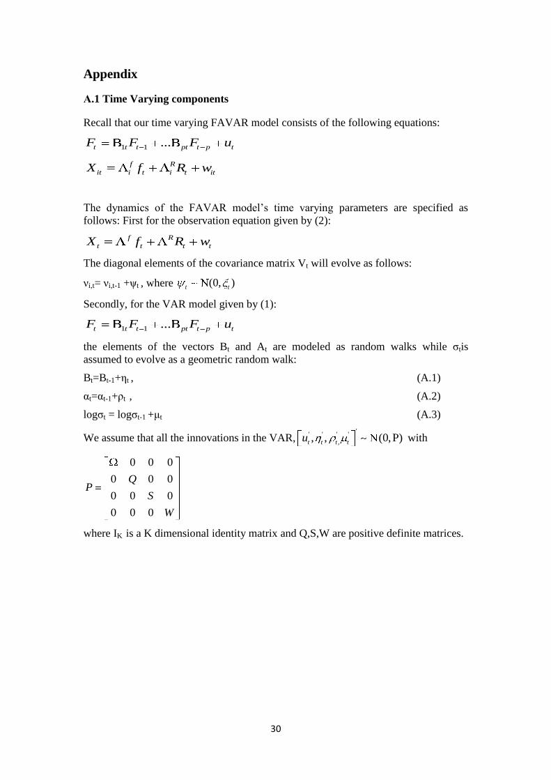
Appendix

Α.1 Time Varying components

Recall that our time varying FAVAR model consists of the following equations:

1 1 ...t t t pt t p tF F F u

f R

it i t i t itX f R w

The dynamics of the FAVAR model’s time varying parameters are specified as

follows: First for the observation equation given by (2):

f R

t t t tX f R w

The diagonal elements of the covariance matrix Vt will evolve as follows:

νi,t= νi,t-1 +ψt , where (0, )tt

Secondly, for the VAR model given by (1):

1 1 ...t t t pt t p tF F F u

the elements of the vectors Bt and At are modeled as random walks while σtis

assumed to evolve as a geometric random walk:

Bt=Bt-1+ηt , (A.1)

αt=αt-1+ρt , (A.2)

logσt = logσt-1 +μt (A.3)

We assume that all the innovations in the VAR,'

' ' ' '

,, , (0,P)t t t tu with

0 0 0

0 0 0

0 0 0

0 0 0

QP

S

W

where IK is a K dimensional identity matrix and Q,S,W are positive definite matrices.

31

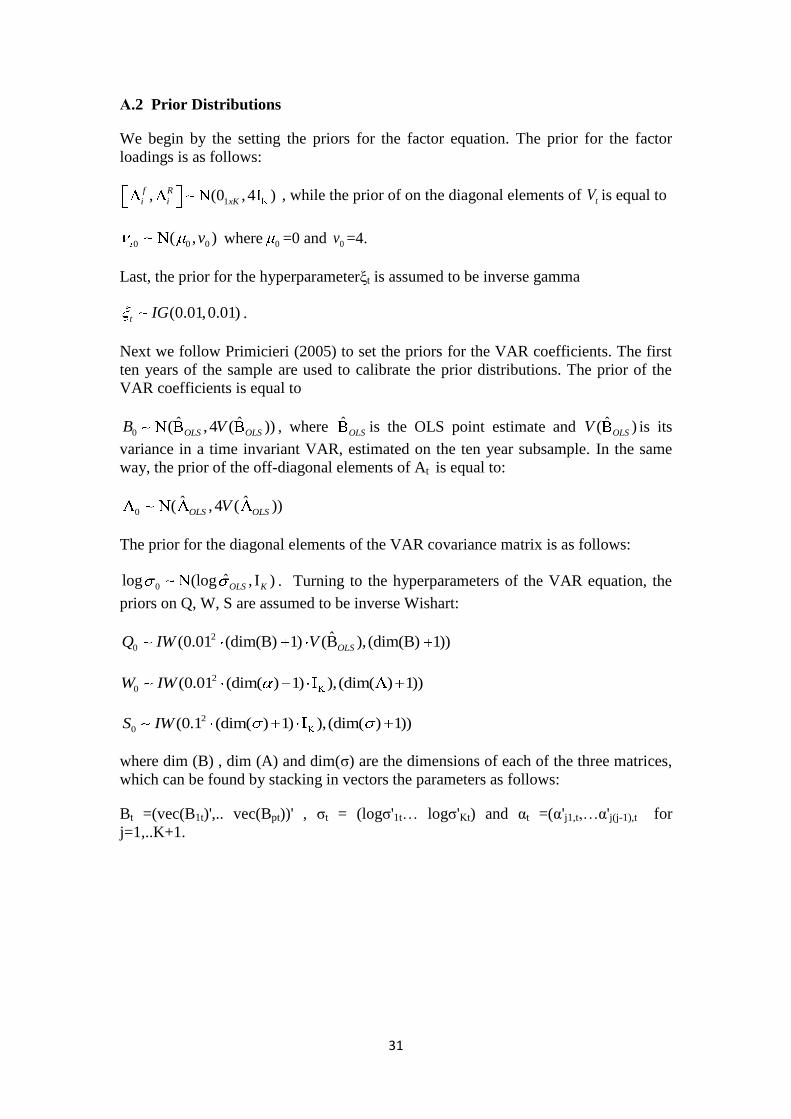
Α.2 Prior Distributions

We begin by the setting the priors for the factor equation. The prior for the factor

loadings is as follows:

1, (0 ,4 )f R

i i xK , while the prior of on the diagonal elements of tV is equal to

0 00 ( , )v where 0 =0 and 0v =4.

Last, the prior for the hyperparameterξt is assumed to be inverse gamma

(0.01,0.01)t IG .

Next we follow Primicieri (2005) to set the priors for the VAR coefficients. The first

ten years of the sample are used to calibrate the prior distributions. The prior of the

VAR coefficients is equal to

0ˆ ˆ( ,4 ( ))OLS OLSVB , where ˆ

OLS is the OLS point estimate and ˆ( )OLSV is its

variance in a time invariant VAR, estimated on the ten year subsample. In the same

way, the prior of the off-diagonal elements of At is equal to:

0ˆ ˆ( , 4 ( ))OLS OLSV

The prior for the diagonal elements of the VAR covariance matrix is as follows:

0ˆlog (log , I )OLS K . Turning to the hyperparameters of the VAR equation, the

priors on Q, W, S are assumed to be inverse Wishart:

2

0ˆ(0.01 (dim(B) 1) (B ), (dim(B) 1))OLSQ IW V

2

0 (0.01 (dim( ) 1) ),(dim( ) 1))W IW

2

0 (0.1 (dim( ) 1) ),(dim( ) 1))S IW

where dim (B) , dim (A) and dim(σ) are the dimensions of each of the three matrices,

which can be found by stacking in vectors the parameters as follows:

Bt =(vec(B1t)',.. vec(Bpt))' , σt = (logσ'1t… logσ'Κt) and αt =(α'j1,t,…α'j(j-1),t for

j=1,..K+1.

32

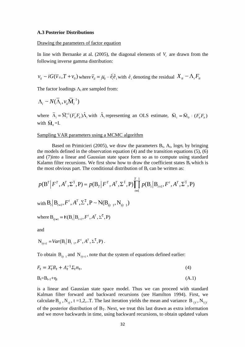
A.3 Posterior Distributions

Drawing the parameters of factor equation

In line with Bernanke at al. (2005), the diagonal elements of tV are drawn from the

following inverse gamma distribution:

0( , )iiiiv iG v T v where'

0ˆ ˆ

ii i iv e e with ˆ ie denoting the residual it itX F

The factor loadings Λi are sampled from:

1( , )iii i iN v

where 1 ' ˆ( )i it iti iF F with ˆ

i representing an OLS estimate, '

0 ( )i it itF F

with 0=I.

Sampling VAR parameters using a MCMC algorithm

Based on Primicieri (2005), we draw the parameters Bt, At, logσt by bringing

the models defined in the observation equation (4) and the transition equations (5), (6)

and (7)into a linear and Gaussian state space form so as to compute using standard

Kalamn filter recursions. We first show how to draw the coefficient states Bt which is

the most obvious part. The conditional distribution of Bt can be written as:

1

1

1

(B , , ,P) (B , , ,P) (B B , , , ,P)T

T T T T T t T

T t t

t

p F A p F A p F A

with 1 1 1B B , , , ,P (B ,N )t T

t t t t t tF A

where11

B (B B , , , ,P)t T

t tt tF A

and

11N (B B , , , ,P)t T

t tt tVar F A .

To obtain 1

Bt t

and 1

Nt t

, note that the system of equations defined earlier:

(4)

Bt=Bt-1+ηt (A.1)

is a linear and Gaussian state space model. Thus we can proceed with standard

Kalman filter forward and backward recursions (see Hamilton 1994). First, we

calculate Bt t

, Nt t

, t =1,2,..T. The last iteration yields the mean and variance B , N

of the posterior distribution of BT. Next, we treat this last drawn as extra information

and we move backwards in time, using backward recursions, to obtain updated values

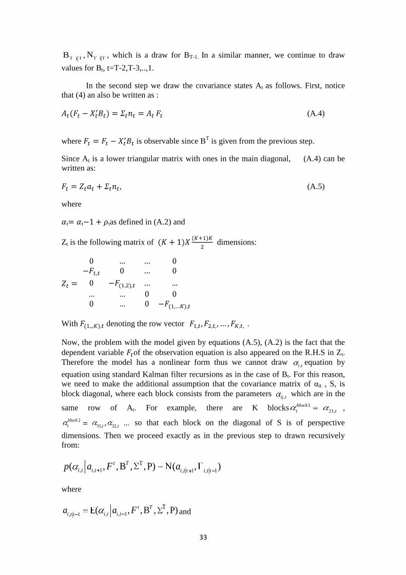
33

1B ,

1N , which is a draw for BT-1. In a similar manner, we continue to draw

values for Bt, t=T-2,T-3,..,1.

In the second step we draw the covariance states At as follows. First, notice

that (4) an also be written as :

(A.4)

where is observable since BT is given from the previous step.

Since At is a lower triangular matrix with ones in the main diagonal, (A.4) can be

written as:

(A.5)

where

t t tas defined in (A.2) and

Zt is the following matrix of dimensions:

With denoting the row vector .

Now, the problem with the model given by equations (A.5), (A.2) is the fact that the

dependent variable of the observation equation is also appeared on the R.H.S in Zt.

Therefore the model has a nonlinear form thus we cannot draw ,i t

equation by

equation using standard Kalman filter recursions as in the case of Bt. For this reason,

we need to make the additional assumption that the covariance matrix of αit , S, is

block diagonal, where each block consists from the parameters ,ij t

which are in the

same row of At. For example, there are K blocks 1

21,

block

t t,

2

31, 32,, ...block

t t t so that each block on the diagonal of S is of perspective

dimensions. Then we proceed exactly as in the previous step to drawn recursively

from:

, , 1 , 1 , 1( , ,B , ,P) ( , )t T

i t i t i t t i t tp a F a

where

, , 1, 1( , ,B , ,P)t T

i t i ti t ta a F and

34

, , 1, 1( , ,B , ,P)t T

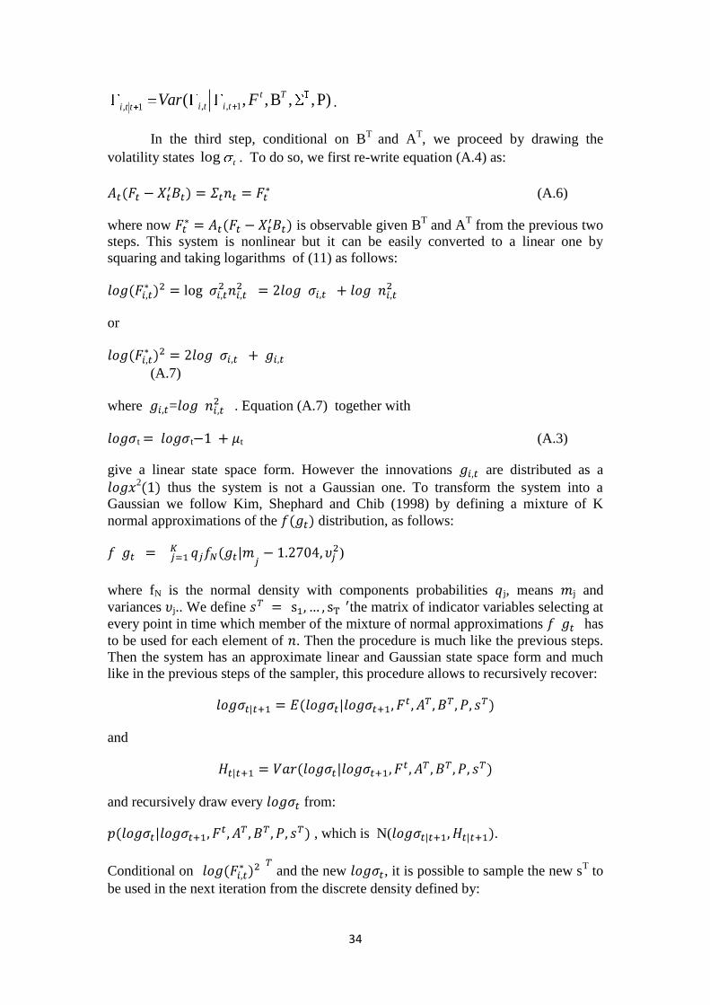
i t i ti t tVar F .

In the third step, conditional on BT

and AT, we proceed by drawing the

volatility states log t . To do so, we first re-write equation (A.4) as:

(A.6)

where now is observable given BT and A

T from the previous two

steps. This system is nonlinear but it can be easily converted to a linear one by

squaring and taking logarithms of (11) as follows:

or

(A.7)

where = . Equation (A.7) together with

t t t (A.3)

give a linear state space form. However the innovations are distributed as a 2

thus the system is not a Gaussian one. To transform the system into a

Gaussian we follow Kim, Shephard and Chib (1998) by defining a mixture of K

normal approximations of the distribution, as follows:

)

where fN is the normal density with components probabilities j, means j and

variances j.. We define the matrix of indicator variables selecting at

every point in time which member of the mixture of normal approximations has

to be used for each element of . Then the procedure is much like the previous steps.

Then the system has an approximate linear and Gaussian state space form and much

like in the previous steps of the sampler, this procedure allows to recursively recover:

and

and recursively draw every from:

, which is N( .

Conditional on and the new , it is possible to sample the new sT to

be used in the next iteration from the discrete density defined by:

35

,

.

Last, we draw the hyperparameters Q, S,W of the covariance matrix P, conditional on

,B , ,t TF , where each hyperparameter has an inverse-Wishart posterior

distribution:

1( , , , ,B , ) ( , ,B , ) ( , ,B , )t T t T t Tp Q S W F p Q F p S F

1... ( , ,B , ) ( , ,B , )t T t T

Kp S F p W F .

36

References

Bernanke, B., Boivin, J. and Eliasz, P., 2005. “Measuring Monetary Policy: A

Factor Augmented Vector Autoregressive (FAVAR) Approach”, Quarterly Journal of

Economics , Vol. 120.

Boivin, J. and Giannoni, M. P., 2006. "Has Monetary Policy Become More

Effective?",Review of Economics and Statistics, Vol. 88(3), pp. 445-462.

Boivin, J. and Giannoni, M, 2008. "Global Forces and Monetary Policy

Effectiveness," NBER Working Papers 13736, National Bureau of Economic

Research, Inc.

Boivin, J., Giannoni, M. and Mojon. B, 2008. "How Has the Euro Changed the

Monetary Transmission Mechanism?”, NBER Macroeconomics Annual 2008,

Volume 23.

Boivin,j., Kiley, M.,T. and Mishkin, F., S., 2010. "How Has the Monetary

Transmission Mechanism Evolved Over Time?", NBER Working Paper No. 15879.

Carter, C. K. and Kohn, R.,, 1994. "On Gibbs sampling for state space

models", Biometrika, Vol. 81, pp. 541–553.

Eickmeier, S., Wolfgang, L.and Massimiliano, M., 2011, "The Changing

International Transmission of Financial Shocks: Evidence from a Classical Time-

Varying FAVAR," CEPR Discussion Papers 8341.

Fukuda, Y., Kimura, Y., Sudo, N., and Ugai, H., 2013. "Cross-country

Transmission Effect of the US Monetary Shock under Global Integration", Bank of

Japan Working Paper Series.

Furceri, D. and Zdzienicka, A., 2010. "Banking Crises and Short and Medium

Term Output Losses in Developing Countries: The Role of Structural and Policy

Variables," MPRA Paper 22078, University Library of Munich, Germany.

Grilli, V. and Roubini, N., 1995. "Liquidity and Exchange Rates: Puzzling

Evidence from the G-7 Countries," Working Papers 95-17, New York University,

Leonard N. Stern School of Business.

Hamilton, J., 1994. Time Series Analysis, Princeton University Press.

Ilzetzki, E. and Jin, K., 2013. "The Puzzling Change in the International

Transmission of U.S. Macroeconomic Policy Shocks", unpublished, London School

of Economics.

Kazi, I., A., Wagan, H. and Akbar, F., 2013. "The changing international

transmission of U.S. monetary policy shocks: Is there evidence of contagion effect on

OECD countries," Economic Modelling, Vol. 30(C), pp. 90-116.

Kim, C. and Nelson, C. R., 1999."Has the U.S. economy become more stable?

A Bayesian approach based on a markov-switching model of the business cycle ", The

Review of Economics and Statistics, Vol. 81, pp. 608–616.

Kim, J., 2001. “International Transmission of US Monetary Policy Shocks:

Evidence from VAR’s”, Journal of Monetary Economics, Vol. 48(2), pp. 339-372.

Kim, S., Shephard, N. and Chib, S., 1998."Stochastic volatility: likelihood

inference and comparison with ARCH models", Review of Economic Studies, Vol. 65,

pp. 361–393.

37

Kim, S. and Yang, D., Y., 2012. "International monetary transmission in East

Asia: Floaters, non-floaters, and capital controls," Japan and the World Economy,

Vol. 24(4), pp.305-316.

Korobilis, D., 2013. "Assessing the Transmission of Monetary Policy Using

Time-varying Parameter Dynamic Factor Models-", Oxford Bulletin of Economics

and Statistics, Vol. 75(2), pp. 157-179.

Kose, M. A., Prasad, E. and Terrones, M., 2007."How Does Financial

Globalization Affect Risk Sharing? Patterns and Channels," IMF Working

Papers 07/238, International Monetary Fund.

Lane, P. R. and Milesi-Ferretti, G. M., 2011. "The Cross-Country Incidence of

the Global Crisis," IMF Economic Review, vol. 59(1), pp. 77-110.

Lutkepohl, H., 2005. New Introduction to Multiple Time Series Analysis,

Springer-Verlag, Berlin.

Miniane, J. and Rogers, J. H., 2007. "Capital Controls and the International

Transmission of U.S. Money Shocks, "Journal of Money, Credit and Banking, Vol.

39(5), pp.1003-1035.

Mumtaz, H. and Surico, P., 2009. "The Transmission of International Shocks:

A Factor-Augmented VAR Approach," Journal of Money, Credit and Banking, vol.

41(s1), pp.71-100.

Mumtaz, H., Zabczyk, P. and Ellis, C., 2011. "What lies beneath? A time-

varying FAVAR model for the UK transmission mechanism," Working Paper

Series 1320, European Central Bank.

Neri, S. and Nobili, A., 2010. "The Transmission of US Monetary Policy to

the Euro Area," International Finance, Wiley Blackwell, Vol. 13(1), pp. 55-78.

Obstfeld, M. and Rogoff, K.,, 1995. "Exchange Rate Dynamics

Redux," Journal of Political Economy”, University of Chicago Press, Vol. 103(3),

pp.624-660.

Primiceri, G., 2005. "Time varying structural vector autoregressions and

monetary policy".Review of Economic Studies, Vol. 72, pp. 821–852.

Rose, A. K. and Spiegel, M. M., 2011."Cross-country causes and

consequences of the crisis: An update," European Economic Review, Vol. 55(3), pp.

309-324.

Sebastian, E., 1985.,"Trends in Real Exchange Rate Behavior in Selected

Developing Countries", World Bank, Country Poliy Department, Discussion Paper

1985-16.

Svensson, L. and van Wijnbergen, S., 1989. "Excess capacity, monopolistic

competition and international transmission of monetary disturbances", Economic

Journal, 99 ,pp. 785–805.

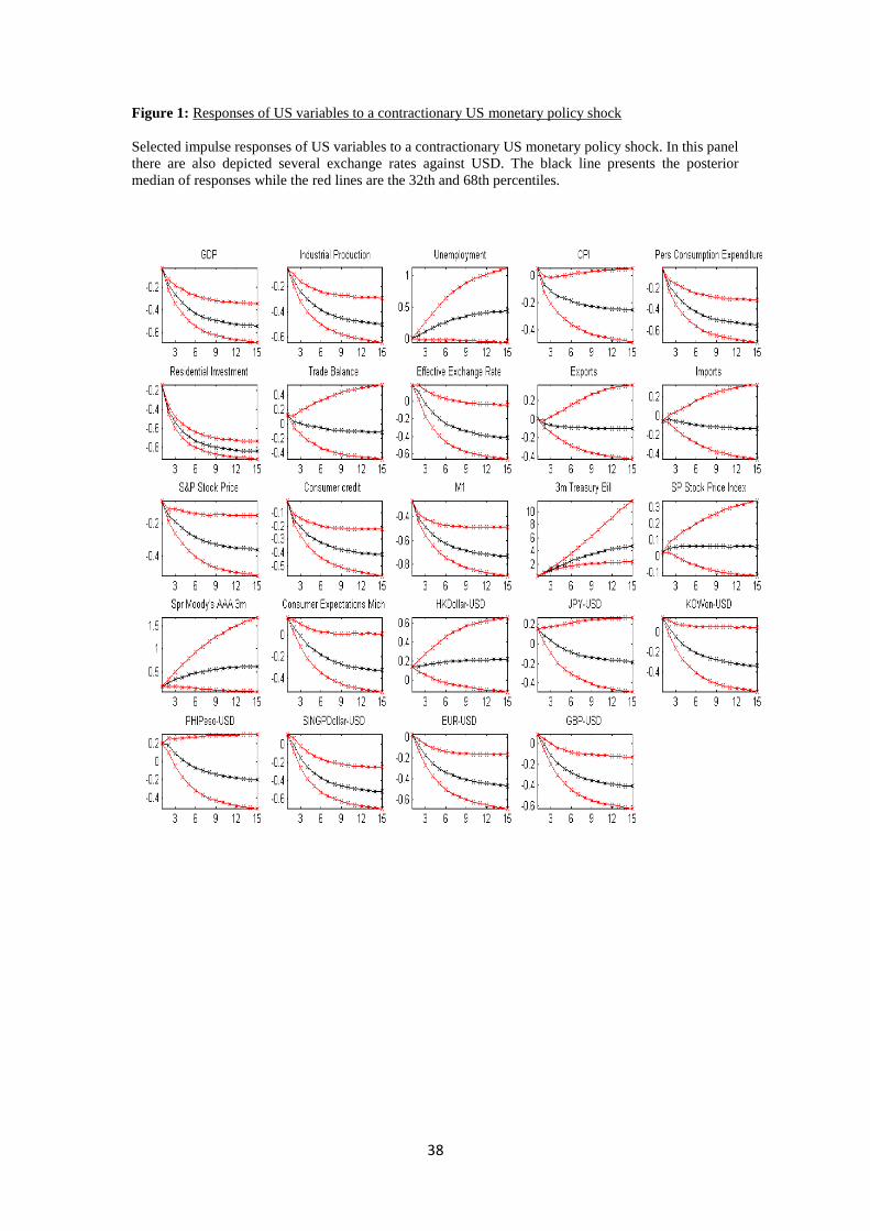
38

Figure 1: Responses of US variables to a contractionary US monetary policy shock

Selected impulse responses of US variables to a contractionary US monetary policy shock. In this panel

there are also depicted several exchange rates against USD. The black line presents the posterior

median of responses while the red lines are the 32th and 68th percentiles.

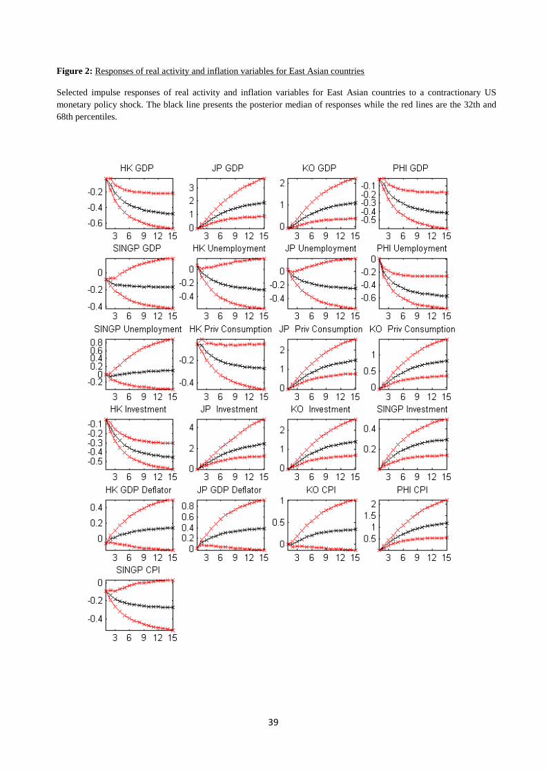
39

Figure 2: Responses of real activity and inflation variables for East Asian countries

Selected impulse responses of real activity and inflation variables for East Asian countries to a contractionary US

monetary policy shock. The black line presents the posterior median of responses while the red lines are the 32th and

68th percentiles.

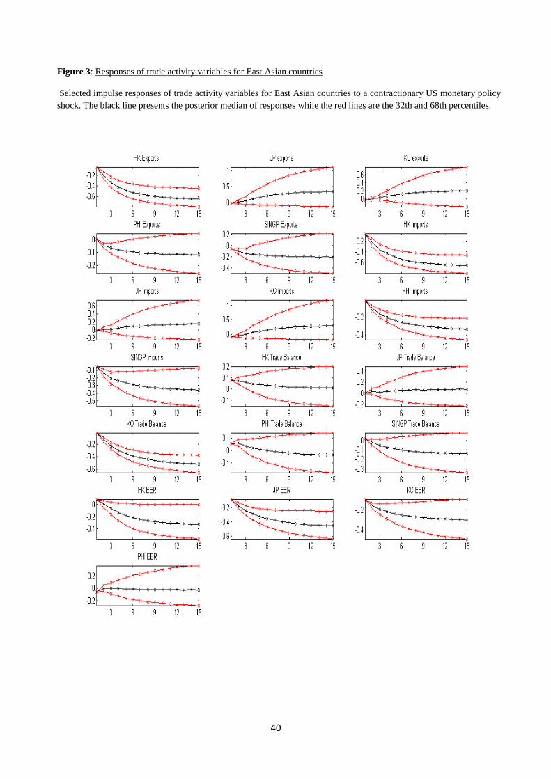
40

Figure 3: Responses of trade activity variables for East Asian countries

Selected impulse responses of trade activity variables for East Asian countries to a contractionary US monetary policy

shock. The black line presents the posterior median of responses while the red lines are the 32th and 68th percentiles.

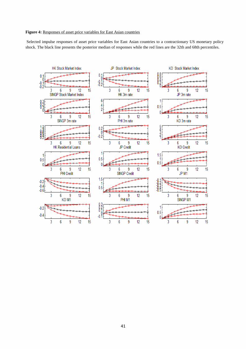
41

Figure 4: Responses of asset price variables for East Asian countries

Selected impulse responses of asset price variables for East Asian countries to a contractionary US monetary policy

shock. The black line presents the posterior median of responses while the red lines are the 32th and 68th percentiles.

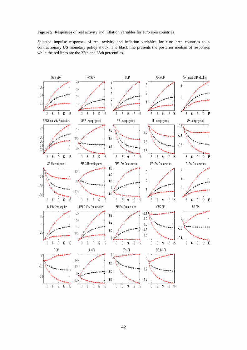
42

Figure 5: Responses of real activity and inflation variables for euro area countries

Selected impulse responses of real activity and inflation variables for euro area countries to a

contractionary US monetary policy shock. The black line presents the posterior median of responses

while the red lines are the 32th and 68th percentiles.

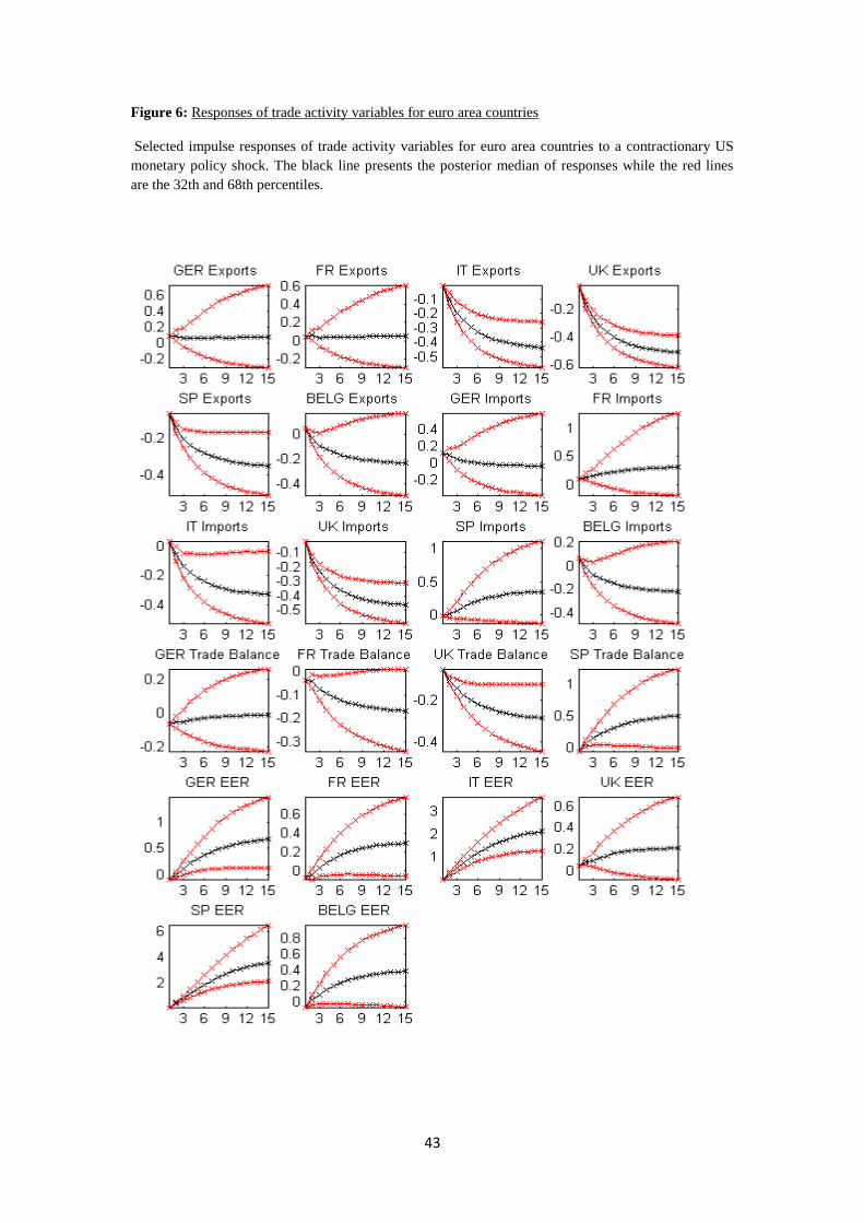
43

Figure 6: Responses of trade activity variables for euro area countries

Selected impulse responses of trade activity variables for euro area countries to a contractionary US

monetary policy shock. The black line presents the posterior median of responses while the red lines

are the 32th and 68th percentiles.

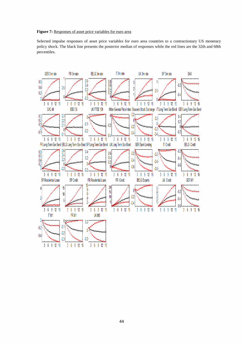
44

Figure 7: Responses of asset price variables for euro area

Selected impulse responses of asset price variables for euro area countries to a contractionary US monetary

policy shock. The black line presents the posterior median of responses while the red lines are the 32th and 68th

percentiles.

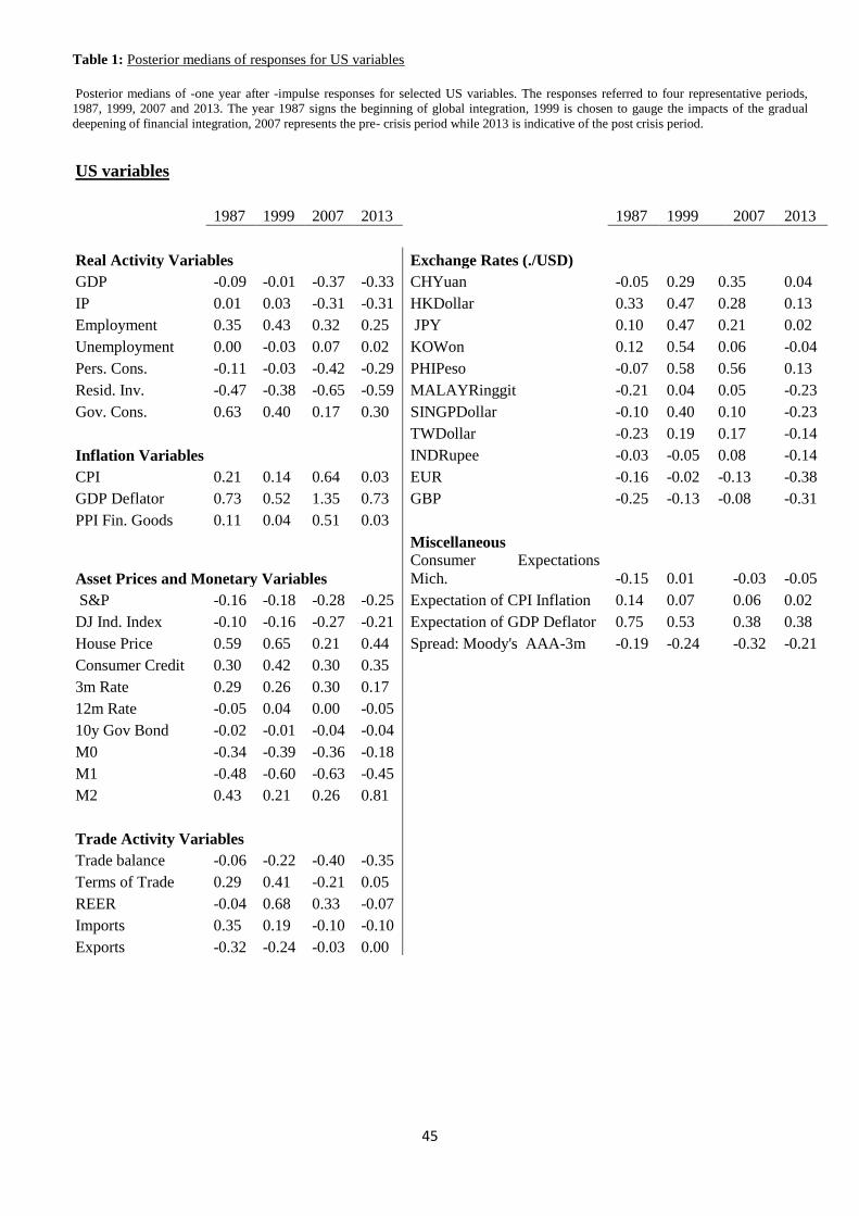
45

Table 1: Posterior medians of responses for US variables

Posterior medians of -one year after -impulse responses for selected US variables. The responses referred to four representative periods,

1987, 1999, 2007 and 2013. The year 1987 signs the beginning of global integration, 1999 is chosen to gauge the impacts of the gradual

deepening of financial integration, 2007 represents the pre- crisis period while 2013 is indicative of the post crisis period.

US variables

1987 1999 2007 2013

1987 1999 2007 2013

Real Activity Variables Exchange Rates (./USD)

GDP -0.09 -0.01 -0.37 -0.33 CHYuan -0.05 0.29 0.35 0.04

IP 0.01 0.03 -0.31 -0.31 HKDollar 0.33 0.47 0.28 0.13

Employment 0.35 0.43 0.32 0.25 JPY 0.10 0.47 0.21 0.02

Unemployment 0.00 -0.03 0.07 0.02 KOWon 0.12 0.54 0.06 -0.04

Pers. Cons. -0.11 -0.03 -0.42 -0.29 PHIPeso -0.07 0.58 0.56 0.13

Resid. Inv. -0.47 -0.38 -0.65 -0.59 MALAYRinggit -0.21 0.04 0.05 -0.23

Gov. Cons. 0.63 0.40 0.17 0.30 SINGPDollar -0.10 0.40 0.10 -0.23

TWDollar -0.23 0.19 0.17 -0.14

Inflation Variables

INDRupee -0.03 -0.05 0.08 -0.14

CPI 0.21 0.14 0.64 0.03 EUR -0.16 -0.02 -0.13 -0.38

GDP Deflator 0.73 0.52 1.35 0.73 GBP -0.25 -0.13 -0.08 -0.31

PPI Fin. Goods 0.11 0.04 0.51 0.03

Miscellaneous

Asset Prices and Monetary Variables

Consumer Expectations

Mich. -0.15 0.01 -0.03 -0.05

S&P -0.16 -0.18 -0.28 -0.25 Expectation of CPI Inflation 0.14 0.07 0.06 0.02

DJ Ind. Index -0.10 -0.16 -0.27 -0.21 Expectation of GDP Deflator 0.75 0.53 0.38 0.38

House Price 0.59 0.65 0.21 0.44 Spread: Moody's AAA-3m -0.19 -0.24 -0.32 -0.21

Consumer Credit 0.30 0.42 0.30 0.35

3m Rate 0.29 0.26 0.30 0.17

12m Rate -0.05 0.04 0.00 -0.05

10y Gov Bond -0.02 -0.01 -0.04 -0.04

M0 -0.34 -0.39 -0.36 -0.18

M1 -0.48 -0.60 -0.63 -0.45

M2 0.43 0.21 0.26 0.81

Trade Activity Variables

Trade balance -0.06 -0.22 -0.40 -0.35

Terms of Trade 0.29 0.41 -0.21 0.05

REER -0.04 0.68 0.33 -0.07

Imports 0.35 0.19 -0.10 -0.10

Exports -0.32 -0.24 -0.03 0.00

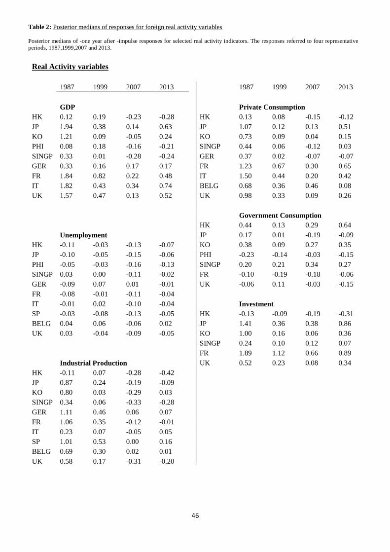
46

Table 2: Posterior medians of responses for foreign real activity variables

Posterior medians of -one year after -impulse responses for selected real activity indicators. The responses referred to four representative

periods, 1987,1999,2007 and 2013.

Real Activity variables

1987 1999 2007 2013

1987 1999 2007 2013

GDP

Private Consumption

HK 0.12 0.19 -0.23 -0.28

HK 0.13 0.08 -0.15 -0.12

JP 1.94 0.38 0.14 0.63

JP 1.07 0.12 0.13 0.51

KO 1.21 0.09 -0.05 0.24

KO 0.73 0.09 0.04 0.15

PHI 0.08 0.18 -0.16 -0.21

SINGP 0.44 0.06 -0.12 0.03

SINGP 0.33 0.01 -0.28 -0.24

GER 0.37 0.02 -0.07 -0.07

GER 0.33 0.16 0.17 0.17

FR 1.23 0.67 0.30 0.65

FR 1.84 0.82 0.22 0.48

IT 1.50 0.44 0.20 0.42

IT 1.82 0.43 0.34 0.74

BELG 0.68 0.36 0.46 0.08

UK 1.57 0.47 0.13 0.52

UK 0.98 0.33 0.09 0.26

Government Consumption

HK 0.44 0.13 0.29 0.64

Unemployment

JP 0.17 0.01 -0.19 -0.09

HK -0.11 -0.03 -0.13 -0.07

KO 0.38 0.09 0.27 0.35

JP -0.10 -0.05 -0.15 -0.06

PHI -0.23 -0.14 -0.03 -0.15

PHI -0.05 -0.03 -0.16 -0.13

SINGP 0.20 0.21 0.34 0.27

SINGP 0.03 0.00 -0.11 -0.02

FR -0.10 -0.19 -0.18 -0.06

GER -0.09 0.07 0.01 -0.01

UK -0.06 0.11 -0.03 -0.15

FR -0.08 -0.01 -0.11 -0.04

IT -0.01 0.02 -0.10 -0.04

Investment

SP -0.03 -0.08 -0.13 -0.05

HK -0.13 -0.09 -0.19 -0.31

BELG 0.04 0.06 -0.06 0.02

JP 1.41 0.36 0.38 0.86

UK 0.03 -0.04 -0.09 -0.05

KO 1.00 0.16 0.06 0.36

SINGP 0.24 0.10 0.12 0.07

FR 1.89 1.12 0.66 0.89

Industrial Production

UK 0.52 0.23 0.08 0.34

HK -0.11 0.07 -0.28 -0.42

JP 0.87 0.24 -0.19 -0.09

KO 0.80 0.03 -0.29 0.03

SINGP 0.34 0.06 -0.33 -0.28

GER 1.11 0.46 0.06 0.07

FR 1.06 0.35 -0.12 -0.01

IT 0.23 0.07 -0.05 0.05

SP 1.01 0.53 0.00 0.16

BELG 0.69 0.30 0.02 0.01

UK 0.58 0.17 -0.31 -0.20

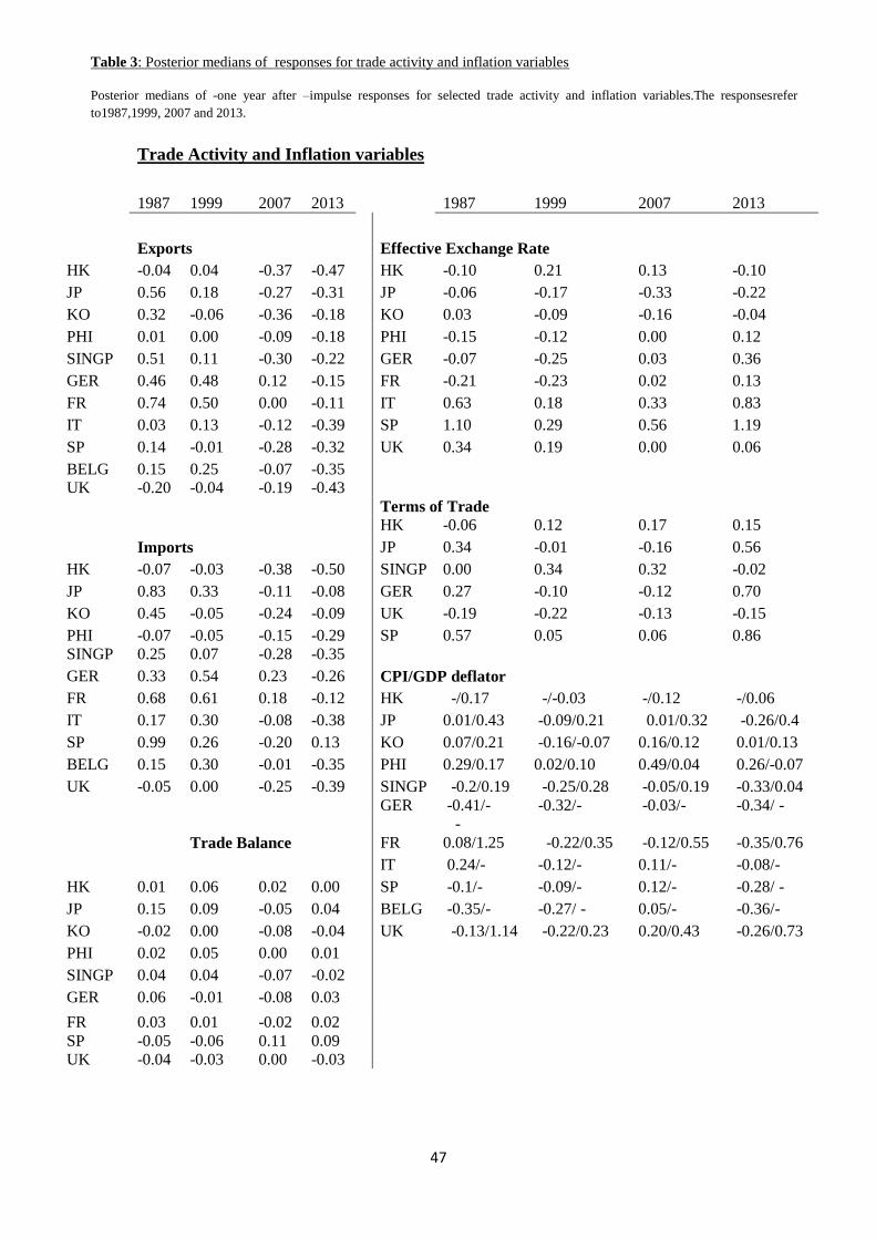
47

Table 3: Posterior medians of responses for trade activity and inflation variables

Posterior medians of -one year after –impulse responses for selected trade activity and inflation variables.The responsesrefer

to1987,1999, 2007 and 2013.

Trade Activity and Inflation variables

1987 1999 2007 2013

1987 1999 2007 2013

Exports

Effective Exchange Rate

HK -0.04 0.04 -0.37 -0.47

HK -0.10 0.21 0.13 -0.10

JP 0.56 0.18 -0.27 -0.31

JP -0.06 -0.17 -0.33 -0.22

KO 0.32 -0.06 -0.36 -0.18

KO 0.03 -0.09 -0.16 -0.04

PHI 0.01 0.00 -0.09 -0.18

PHI -0.15 -0.12 0.00 0.12

SINGP 0.51 0.11 -0.30 -0.22

GER -0.07 -0.25 0.03 0.36

GER 0.46 0.48 0.12 -0.15

FR -0.21 -0.23 0.02 0.13

FR 0.74 0.50 0.00 -0.11

IT 0.63 0.18 0.33 0.83

IT 0.03 0.13 -0.12 -0.39

SP 1.10 0.29 0.56 1.19

SP 0.14 -0.01 -0.28 -0.32

UK 0.34 0.19 0.00 0.06

BELG 0.15 0.25 -0.07 -0.35

UK -0.20 -0.04 -0.19 -0.43

Terms of Trade

HK -0.06 0.12 0.17 0.15

Imports

JP 0.34 -0.01 -0.16 0.56

HK -0.07 -0.03 -0.38 -0.50

SINGP 0.00 0.34 0.32 -0.02

JP 0.83 0.33 -0.11 -0.08

GER 0.27 -0.10 -0.12 0.70

KO 0.45 -0.05 -0.24 -0.09

UK -0.19 -0.22 -0.13 -0.15

PHI -0.07 -0.05 -0.15 -0.29

SP 0.57 0.05 0.06 0.86

SINGP 0.25 0.07 -0.28 -0.35

GER 0.33 0.54 0.23 -0.26

CPI/GDP deflator

FR 0.68 0.61 0.18 -0.12

HK -/0.17 -/-0.03 -/0.12 -/0.06

IT 0.17 0.30 -0.08 -0.38

JP 0.01/0.43 -0.09/0.21 0.01/0.32 -0.26/0.4

SP 0.99 0.26 -0.20 0.13

KO 0.07/0.21 -0.16/-0.07 0.16/0.12 0.01/0.13

BELG 0.15 0.30 -0.01 -0.35

PHI 0.29/0.17 0.02/0.10 0.49/0.04 0.26/-0.07

UK -0.05 0.00 -0.25 -0.39

SINGP -0.2/0.19 -0.25/0.28 -0.05/0.19 -0.33/0.04

GER -0.41/- -0.32/- -0.03/- -0.34/ -

Trade Balance

FR

-

0.08/1.25 -0.22/0.35 -0.12/0.55 -0.35/0.76

IT 0.24/- -0.12/- 0.11/- -0.08/-

HK 0.01 0.06 0.02 0.00

SP -0.1/- -0.09/- 0.12/- -0.28/ -

JP 0.15 0.09 -0.05 0.04

BELG -0.35/- -0.27/ - 0.05/- -0.36/-

KO -0.02 0.00 -0.08 -0.04

UK -0.13/1.14 -0.22/0.23 0.20/0.43 -0.26/0.73

PHI 0.02 0.05 0.00 0.01

SINGP 0.04 0.04 -0.07 -0.02

GER 0.06 -0.01 -0.08 0.03

FR 0.03 0.01 -0.02 0.02

SP -0.05 -0.06 0.11 0.09

UK -0.04 -0.03 0.00 -0.03

48

Table 4: Posterior medians of responses for selected asset price variables

Posterior medians of one-year-after-impulse responses for selected asset price variables. The responses referred to four

representative periods, 1987,1999, 2007 and 2013.

Asset Price variables

1987 1999 2007 2013

1987 1999 2007 2013

3 month interest rate

Residential Loans/Consumer Credit

HK 0.24 0.22 0.24 0.14

JP 0.17 0.02 0.09 0.04

HK 0.43/- -0.16/- 0.06/- 0.13/ -

KO 0.01 0.03 0.06 -0.03

JP -/0.23 -/-0.17 -/0.00 -/0.22

PHI 0.07 0.09 0.06 -0.01

KO -/0.56 -/0.40 -/0.46 -/0.45

SINGP 0.22 0.18 0.26 0.14

PHI - /-0.36 - /-0.14 -/0.01 -/-0.27

GER 0.04 0.02 0.10 -0.02

SINGP -/0.12 /0.06 - /0.57 -/0.57

FR 0.11 0.03 0.11 0.02

GER -0.04/-0.16 -0.13/-0.11 -0.28/0.00 -0.34/-0.22

IT 0.11 0.04 0.09 0.02

FR 1.25/2.16 0.88/1.12 1.25/1.86 1.02/1.91

SP 0.16 0.05 0.09 0.04

IT -/0.69 -/0.17 -/0.43 -/0.42

BELG 0.11 0.04 0.11 0.01

SP 0.96/1.62 1.23/1.44 1.01/1.76 0.53/1.44

UK 0.19 0.13 0.20 0.09

BELG -/-0.46 /-0.39 -/-0.29 -/-0.35

UK -/1.21 -/0.53 -/0.60 -/0.76

Stock Market Index

HK 0.04 -0.04 -0.08 -0.07

M0/M1

JP 0.21 0.15 -0.12 -0.04

JP 0.64/-0.16 0.39/-0.12 0.24/-0.32 0.46/-0.28

KO 0.35 -0.07 -0.21 0.07

KO 0.13/0.09 0.15/-0.09 -0.04/-0.33 -0.06/ -0.24

SINGP 0.20 -0.01 -0.11 0.01

PHI 0.33/0.26 0.30/0.27 0.03/0.05 0.05 /0.06

GER 0.10 0.21 0.20 0.11

SINGP 0.19/0.16 0.02/-0.17 0.08/0.01 0.14/0.26

FR 0.16 0.23 0.12 0.09

GER 0.21/-0.13 0.31/0.07 0.14/-0.11 -0.04/-0.21

IT -0.05 0.03 -0.16 -0.11

IT -/0.08 -/0.20 -/-0.16 -/-0.21

BELG -0.02 0.09 0.13 0.09

FR -/0.11 -/0.14 -/-0.19 -/-0.18

SP 0.12 0.11 0.05 0.11

UK 0.22/- 0.24/- -0.09/- 0.02/-

UK 0.08 0.08 -0.02 -0.03

Long Term Interest Rate

JP 0.13 0.03 0.09 0.02

GER 0.10 0.06 0.07 -0.02

FR 0.16 0.06 0.08 0.01

IT 0.09 0.01 0.06 0.00

BELG 0.13 0.04 0.07 0.00

SP 0.11 0.03 0.03 0.01

UK 0.08 0.05 0.07 0.02

49

BANK OF GREECE WORKING PAPERS

173. Du Caju, P., T. Kosma, M. Lawless, J. Messina, T. Rõõm, Why Firms Avoid

Cutting Wages: Survey Evidence From European Firms”, January 2014.

174. Mitrakos, T., “Inequality, Poverty and Social Welfare in Greece:

Distributional Effects of Austerity”, February 2014.

175. Lazaretou, S., “Η Έξυπνη Οικονομία: «Πολιτιστικές» και «Δημιουργικές»

Βιομηχανίες Στην Ελλάδα Μπορούν Να Αποτελέσουν Προοπτική Εξόδου

Από Την Κρίση”, February 2014.

176. Chouliarakis, G., and S. Lazaretou, “Déjà Vu? The Greek Crisis Experience,

the 2010s Versus the 1930s. Lessons From History”, February 2014.

177. Tavlas, G.S., “In Old Chicago: Simons, Friedman and The Development of

Monetary-Policy Rules”, March 2014.

178. Bardakas, C. I., “Financing Exports of Goods: a Constraint on Greek

Economic Growth, March 2014.

179. Tagkalakis, O.A,. “Financial Stability Indicators and Public Debt

Developments”, May 2014.

180. Kaplanoglou, G., V. T., Rapanos , and I.C, Bardakas, “Does Fairness Matter

for the Success of Fiscal Consolidation?”, May 2014.

181. Tagkalakis, O. A., “The Determinants of VAT Revenue Efficiency: Recent

Evidence from Greece”, May 2014.

182. Papageorgiou, D., “BoGGEM: A Dynamic Stochastic General Equilibrium

Model for Policy Simulations”, May 2014.

183. Tsionas, E.G., “On Modeling Banking Risk”, May 2014.

184. Louzis, P.D., “Macroeconomic and credit forecasts in a small economy during

crisis: a large Bayesian VAR approach”, June 2014.

185. Adam, A., and T., Moutos, “Industry-Level Labour Demand ElasticitiesAcross

the Eurozone: Will There Be Any Gain After the Pain of Internal

Devaluation?” July, 2014.

186. Tagkalakis, O.A., “Fiscal Policy, Net Exports, and the Sectoral Composition

of Output in Greece”, September 2014.

187. Hondroyiannis, G. and D., Papaoikonomou, “When Does it Pay To Tax?

Evidence from State-Dependent Fiscal Multipliers in the Euro Area”, October

2014.

188. Charalambakis, C. E., “On Corporate Financial Distress Prediction: What Can

we Learn From Private Firms in a Small Open Economy?, November 2014.

189. Pagratis, S., E., Karakatsani and E. Louri, “Bank Leverage and Return on

Equity Targeting: Intrinsic Procyclicality of Short-Term Choices”, November

2014.