GENERALIZED STATISTICAL ARBITRAGE CONCEPTS AND …
24
GENERALIZED STATISTICAL ARBITRAGE CONCEPTS AND RELATED GAIN STRATEGIES CHRISTIAN REIN, LUDGER R ¨ USCHENDORF, AND THORSTEN SCHMIDT Abstract. The notion of statistical arbitrage introduced in Bondarenko (2003) is generalized to statistical G -arbitrage corresponding to trading strategies which yield positive gains on average in a class of scenarios described by a σ-algebra G . This notion contains classical arbitrage as a special case. Admitting general static payoffs as generalized strategies, as done in Kassberger and Liebmann (2017) in the case of one pricing measure, leads to the notion of generalized statistical G -arbitrage. We show that even under standard no-arbitrage there may exist generalized gain strategies yielding positive gains on average under the specified scenarios. In the first part of the paper we prove that the characterization in Bondarenko (2003), no statistical arbitrage being equivalent to the existence of an equivalent local martingale measure with a path-independent density, is not correct in general. We establish that this equivalence holds true in complete markets and we derive a general sufficient condition for statistical G -arbitrages. As a main result we derive the equivalence of no statistical G -arbitrage to no generalized statistical G -arbitrage. In the second part of the paper we construct several classes of profitable generalized strategies with respect to various choices of the σ-algebra G . In particular, we consider several forms of embedded binomial strategies and follow-the-trend strategies as well as partition-type strategies. We study and compare their behaviour on simulated data and also evaluate their performance on market data. 1. Introduction Since the mid-1980s trading strategies which offer profits on average in comparison to little remaining risk have been implemented and analyzed. The starting point were pairs trading strategies, see Gatev et al. (2006) for an historic account and further details. In this strategy one trades two stocks whose prices have a high historic correlation and whose spread widened recently, by buying the loser and shorting the winner. Many variants of this simple strategy followed, see Krauss (2017) and Lazzarino et al. (2018) for surveys and guides to the literature. This raised interest in a deeper theoretical understanding of these approaches. In this paper, we elaborate and generalize the notion of statistical arbitrage (SA) introduced in Bondarenko (2003). The author considers a finite horizon market, represented by the price process of the assets (S t ) t∈[0,T ] . A trading strategy with zero initial cost is called statistical arbitrage if (i) the expected payoff is positive and, (ii) the expected payoff is non-negative conditional on S T . Unlike pure arbitrage strategies, a statistical arbitrage can have negative payoffs provided the average payoff in each final state is non-negative. This concept supplements previous forms of restrictions like ‘good deals’ or opportunities with high Sharpe ratios or with high utility (see Hansen and Jagannathan (1991), Cochrane and Saa-Requejo (2000) and ˇ Cern` y and Hodges (2002)) or ‘approximate arbitrage opportunities’ and investment opportunities with a high gain-loss ratio (see Bernardo and Ledoit (2000)). All these restrictions lead to essential reductions of the pricing intervals. Bondarenko (2003) discusses the concept of statistical arbitrage in connection with various forms of risk preferences, w.r.t. the solution of the joint hypothesis problem, for tests of the efficient market hypothesis (EMH) and the efficient learning market (ELM). The main economic assumption introduced by Bondarenko is the assumption that the pricing kernel is path independent, i.e. it is a function depending only on the final state of the underlying price model but not depending on the whole Date : February 2, 2021. The first two authors acknowledge gratefully support by the DFG project RU 704/11-1. The last author acknowledges support by the DFG project SCHM 2016/13-1 and thanks the Freiburg Institute for Advanced Studies (FRIAS) for generous hospitality and support. The authors are grateful to the two reviewers, the Associate Editor, and the Editor, whose comments were helpful to improve the paper. 1
Transcript of GENERALIZED STATISTICAL ARBITRAGE CONCEPTS AND …
GENERALIZED STATISTICAL ARBITRAGE CONCEPTS AND RELATED
GAIN STRATEGIES
CHRISTIAN REIN, LUDGER RUSCHENDORF, AND THORSTEN SCHMIDT
Abstract. The notion of statistical arbitrage introduced in Bondarenko (2003) is generalized tostatistical G -arbitrage corresponding to trading strategies which yield positive gains on average in aclass of scenarios described by a σ-algebra G . This notion contains classical arbitrage as a specialcase. Admitting general static payoffs as generalized strategies, as done in Kassberger and Liebmann
(2017) in the case of one pricing measure, leads to the notion of generalized statistical G -arbitrage.We show that even under standard no-arbitrage there may exist generalized gain strategies yieldingpositive gains on average under the specified scenarios.
In the first part of the paper we prove that the characterization in Bondarenko (2003), nostatistical arbitrage being equivalent to the existence of an equivalent local martingale measure witha path-independent density, is not correct in general. We establish that this equivalence holds true
in complete markets and we derive a general sufficient condition for statistical G -arbitrages. Asa main result we derive the equivalence of no statistical G -arbitrage to no generalized statisticalG -arbitrage.
In the second part of the paper we construct several classes of profitable generalized strategies
with respect to various choices of the σ-algebra G . In particular, we consider several forms ofembedded binomial strategies and follow-the-trend strategies as well as partition-type strategies.We study and compare their behaviour on simulated data and also evaluate their performance onmarket data.
1. Introduction
Since the mid-1980s trading strategies which offer profits on average in comparison to little remainingrisk have been implemented and analyzed. The starting point were pairs trading strategies, see Gatevet al. (2006) for an historic account and further details. In this strategy one trades two stocks whoseprices have a high historic correlation and whose spread widened recently, by buying the loser andshorting the winner. Many variants of this simple strategy followed, see Krauss (2017) and Lazzarinoet al. (2018) for surveys and guides to the literature. This raised interest in a deeper theoreticalunderstanding of these approaches.
In this paper, we elaborate and generalize the notion of statistical arbitrage (SA) introduced inBondarenko (2003). The author considers a finite horizon market, represented by the price process ofthe assets (St)t∈[0,T ]. A trading strategy with zero initial cost is called statistical arbitrage if
(i) the expected payoff is positive and,(ii) the expected payoff is non-negative conditional on ST .
Unlike pure arbitrage strategies, a statistical arbitrage can have negative payoffs provided the averagepayoff in each final state is non-negative. This concept supplements previous forms of restrictions like‘good deals’ or opportunities with high Sharpe ratios or with high utility (see Hansen and Jagannathan(1991), Cochrane and Saa-Requejo (2000) and Cerny and Hodges (2002)) or ‘approximate arbitrageopportunities’ and investment opportunities with a high gain-loss ratio (see Bernardo and Ledoit(2000)). All these restrictions lead to essential reductions of the pricing intervals.
Bondarenko (2003) discusses the concept of statistical arbitrage in connection with various formsof risk preferences, w.r.t. the solution of the joint hypothesis problem, for tests of the efficient markethypothesis (EMH) and the efficient learning market (ELM). The main economic assumption introducedby Bondarenko is the assumption that the pricing kernel is path independent, i.e. it is a functiondepending only on the final state of the underlying price model but not depending on the whole
Date: February 2, 2021.The first two authors acknowledge gratefully support by the DFG project RU 704/11-1. The last author acknowledges
support by the DFG project SCHM 2016/13-1 and thanks the Freiburg Institute for Advanced Studies (FRIAS) for
generous hospitality and support. The authors are grateful to the two reviewers, the Associate Editor, and the Editor,
whose comments were helpful to improve the paper.1
2 CHRISTIAN REIN, LUDGER RUSCHENDORF, AND THORSTEN SCHMIDT
history. This assumption implies that the payoff process deflated by the conditional risk neutraldensity of the final state is a martingale, i.e. has no systematic trend. The main result in (Bondarenko,2003, Proposition 1) states that the existence of a path-independent pricing kernel is equivalent to theabsence of SA strategies.
Hogan et al. (2004) introduce a related approach which considers on an infinite time horizonwith trading strategies achieving positive gains on average together with vanishing risk, both in anasymptotic sense. See also Elliott et al. (2005); Avellaneda and Lee (2010).
In Section 2 we generalize the concept of statistical arbitrage. Starting from a σ-field G , a statisticalG -arbitrage is a trading strategy with positive expected gain, conditional on G . The existence of apricing measure with G -measurable density implies absence of statistical G -arbitrage. Investigatingin detail a class of trinomial models we find that the converse direction in Bondarenko’s equivalencetheorem is not valid in general. Kassberger and Liebmann (2017) introduced and characterizedstatistical G -arbitrage w.r.t. generalized (static) strategies in the case where one pricing measure isfixed. In Section 3 we introduce generalized trading strategies including also static or semi-staticstrategies and derive various characterizations of the corresponding SA concepts for the class of allmartingale pricing measures. In Section 4 we fully characterize SA for two-period binomial models andconstruct statistical arbitrage strategies. These results are used in Section 5 to construct for discrete-and continuous-time models various SA-strategies. We test them in several examples and give anapplication to market data. A basic class of strategies is obtained by embedding binomial tradingstrategies into the continuous time models using first-hitting times. Further classes are strategiesinduced by partitioning the path space and strategies which follow some trend in the data. Several oftheses strategies are examined and compared.
2. Statistical G -arbitrage strategies
Consider a filtered probability space (Ω,F , P ) with a filtration F = (Ft)0≤t≤T and a finite timehorizon T . The filtration is assumed to satisfy the usual conditions, i. e. it is right continuous andF0 contains all null sets of F : if B ⊂ A ∈ F and P (A) = 0 then B ∈ F0. We also suppose thatF = FT .
We follow the classical approach to financial markets as for example in Delbaen and Schachermayer(2006). The market itself is given by a Rd+1-valued locally bounded semi-martingale S = (S0, . . . , Sd),i.e. there exists a sequence of stopping times (Tn)n≥1 tending to ∞ a.s. and a sequence (Kn)n≥1 ofpositive constants, such that |S1J0,TnK| < Kn, n ≥ 1. The numeraire S0 is set equal to one, such thatthe prices are considered as already discounted.
A dynamic trading strategy φ is an S-integrable and predictable process such that the associatedvalue process V = V (φ) is given by
Vt(φ) =
∫ t
0
φs dSs, 0 ≤ t ≤ T. (1)
The trading strategy φ is called a-admissible if φ0 = 0 and Vt(φ) ≥ −a for all t ≥ 0. φ is calledadmissible if it is admissible for some a > 0. We further assume that the market is free of arbitrage inthe sense of no free lunch with vanishing risk (NFLVR), which is equivalent to the existence of anequivalent local martingale measure Q, see Delbaen and Schachermayer (2006). Here, a measure Qwhich is equivalent to P , Q ∼ P , such that S is an F-(local) martingale with respect to Q is calledequivalent (local) martingale measure, EMM (ELMM). Let M e denote the set of all equivalent localmartingale measures.
A statistical arbitrage is a dynamic trading strategy which is on average profitable, conditional onthe final state of the economy ST . More generally, we consider a general σ-field G ⊂ FT and considerstrategies which are on average profitable conditional on G . For example, G could be generated bythe event ST > K. We call such strategies G -arbitrage strategies. Sometimes we call a statisticalG -arbitrage strategy also a G -profitable strategy or G -arbitrage, for short. By E we denote expectationwith respect to the reference measure P .
GENERALIZED STATISTICAL ARBITRAGE CONCEPTS 3
Definition 2.1. Let G ⊆ FT be a σ-algebra. An admissible dynamic trading strategy φ is called astatistical G -arbitrage strategy, if
i) E[VT (φ)|G ] ≥ 0, P -a.s.,ii) E[VT (φ)] > 0.
LetSA(G ) := φ : φ is a G -arbitrage
denote the set of all statistical G -arbitrage strategies. The market model satisfies the condition of nostatistical G -arbitrage NSA(G ) if
SA(G ) = ∅.
For G = FT , NSA(G ) is equivalent to the classical no-arbitrage condition (NA) since thenE[VT (φ)|G ] = VT (φ). Recall that NA is implied by NFLVR. If G = σ(ST ), one recovers the notion ofstatistical arbitrage introduced in Bondarenko (2003) and we use the notation NSA = NSA(σ(ST )).
A further interesting type of examples is the case where G = σ(ST ∈ Ki, i ∈ I), Kii∈I beinga partition of the state space, such that a statistical arbitrage offers a gain in any ST ∈ Ki onaverage, i.e. E[VT (φ)|ST ∈ Ki] ≥ 0 for all i ∈ I s.t. P (ST ∈ Ki) > 0. Similarly one can also considerpath-dependent strategies, like for example G = σ(max0≤t≤T St ∈ Ki, i ∈ I).
Remark 2.2. (a) Some immediate consequences of Definition 2.1 are the following:(i) The tower property of conditional expectations yields that larger σ-fields G allow for
fewer profitable G -arbitrage strategies i. e. G1 ⊂ G2 implies that SA(G2) ⊂ SA(G1). As aconsequence we get that in this case
NSA(G1) ⇒ NSA(G2). (2)
(ii) If G = ∅,Ω, then φ ∈ SA(G ) iff EP [VT (φ)] > 0.(b) The general approach to good-deal bounds in Cerny and Hodges (2002) allows to consider statistical
arbitrages as a special case: indeed, if we define
A = Z : E[Z|G ] ≥ 0 and E[Z] > 0as set of good deals then a statistical G -arbitrage φ is a good-deal strategy if VT (φ) ∈ A. Thecorresponding good-deal pricing bound for an option X is given by
π(X) = infx : ∃φ admissible s.t. X + x+ VT (φ) ∈ A,i.e. the smallest price x, such that the portfolio of the option, the price x and the value from ahedging strategy VT (φ) is a good deal.
Remark 2.3 (Connection to other concepts of statistical arbitrage). A comprehensive overview ofthe variety of statistical arbitrage definitions can be found in Lazzarino et al. (2018). This overviewshows that in one group of definitions a particular strategy is considered (for example, pairs trading,cointegration strategies, or arbitrage testing strategies) and statistical arbitrage corresponds to theperformance in simulations or on real data. A general and far reaching analysis of statistical arbitragestrategies based on the excursion theory of processes (in particular of Markov processes) is given inthe recent preprint Ananova et al. (2020).
In comparison to that, the definitions of Bondarenko (2003) and Hogan et al. (2004) and theirgeneralizations are more conceptual. They are not restricted to particular strategies, but ask thequestion: is there a general trading strategy available implying arbitrage in the sense of positiveconditional expectation.
These two concepts can be linked as follows: note that the definition of Bondarenko considers afinite time horizon. Iterating this strategy over time under some kind of stationarity or mean reversion,one gets as a consequence a statistical arbitrage strategy in the asymptotic sense of Hogan et al. Themain technical tool to achieve this are boundary crossing probabilities and in particular the resultsfrom excursion theory as in Ananova et al. From this viewpoint, the definition of statistical arbitrageas in the (weak) sense of Bondarenko is also of interest for the asymptotic definition in Hogan et al.
Also for a finite time horizon statistical arbitrage can be realized by repetition making use of alaw of large numbers. We use this principle in examples in Section 5 of this paper. There we moregenerally construct profitable strategies in the sense of measuring statistical arbitrage with respect toseveral classes of σ-fields.
4 CHRISTIAN REIN, LUDGER RUSCHENDORF, AND THORSTEN SCHMIDT
The connection of the statistical arbitrage notions of Bondarenko and Hogan et al. to the abovementioned group of definitions focussing on particular strategies (pairs trading, cointegration, etc.,as in Lazzarino et al. (2018) or Avellaneda and Lee (2010)), is as follows: in these works severalstrategies are compared on the basis of the realized Sharpe ratio. This is in agreement with theasymptotic viewpoint in Hogan et al. who require, in economic terms, that a statistical arbitrageopportunity produces riskless incremental profit with an persisting positive Sharpe ratio in the limit.Therefore, also the Bondarenko notion, even if seemingly formulated in a weak sense, can be seenin close connection with the other more specific statistical arbitrage notions in the literature andtherefore, is also well motivated from a practical point of view.
Proposition 1 in Bondarenko (2003) states that (in discrete time), NSA is equivalent to the existenceof an equivalent martingale measure Q with path independent density Z, i. e.
dQ
dP= Z ∈ σ(ST ), (3)
where we use the notation Z ∈ σ(ST ) for Z being σ(ST )-measurable. We establish in Section 2.2, thatthis equivalence is incorrect in general. However, in Section 3 we show that this equivalence holds ifthe market is complete. We also establish that the statistical no G -arbitrage NSA(G )-condition isequivalent to the corresponding no-G -arbitrage condition w.r.t. generalized strategies. In Sections 4and 5 we explicitly construct statistical arbitrages.
On the other side, existence of an equivalent martingale measure with path independent density Zimplies that NSA holds without further assumptions. This also holds true for the generalized notionNSA(G ), as we show next.
Theorem 2.4. If there exists Q ∈M e such that dQdP is G -measurable, then NSA(G ) holds.
Proof. The proof follows from the Bayes-formula for conditional expectations. We denote by Lb =
Lb(P ) the set of random variables bounded P -almost surely from below. If Z = dQdP ∈ G , then for any
X ∈ Lb it holds that
EQ[X |G ] =EP [XZ |G ]
EP [Z |G ]= EP [X |G ]. (4)
If there would be a statistical arbitrage strategy φ with EP [X |G ] ≥ 0 and EP [X] > 0, whereX = VT (φ), then, by (4),
EQ[X |G ] ≥ 0, Q-a.s.
Moreover, since φ is admissible, V (φ) is a Q-supermartingale by Fatou’s lemma, and we obtain that
EQ[X] = EQ[VT (φ)] ≤ V0(φ) = 0. (5)
Hence,
0 = EQ[X |G ] = EP [X |G ]
in contradiction to EP [X] > 0.
Remark 2.5 (Alternative admissible strategies). An inspection of the proof, in particular Equation(5), shows that the claim also holds when we consider as admissible such strategies φ for which V (φ)is a Q-supermartingale.
In the following we establish that the converse direction in the Bondarenko result is not true. Forthe construction of a counterexample we characterize next statistical arbitrage in a certain class oftrinomial models.
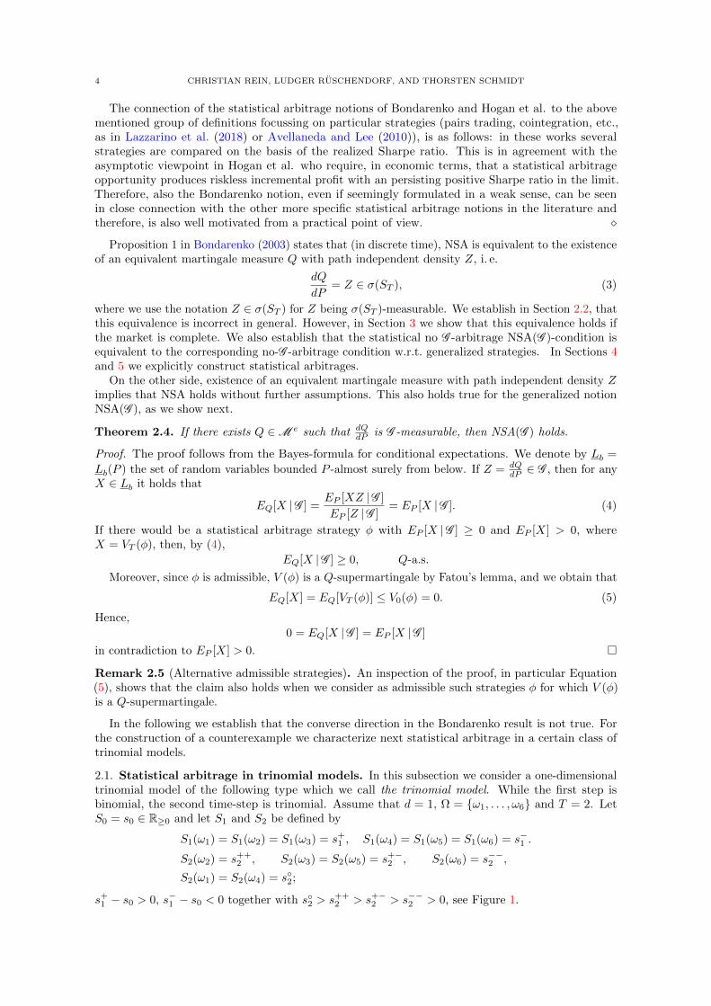
2.1. Statistical arbitrage in trinomial models. In this subsection we consider a one-dimensionaltrinomial model of the following type which we call the trinomial model. While the first step isbinomial, the second time-step is trinomial. Assume that d = 1, Ω = ω1, . . . , ω6 and T = 2. LetS0 = s0 ∈ R≥0 and let S1 and S2 be defined by
S1(ω1) = S1(ω2) = S1(ω3) = s+1 , S1(ω4) = S1(ω5) = S1(ω6) = s−1 .
S2(ω2) = s++2 , S2(ω3) = S2(ω5) = s+−
2 , S2(ω6) = s−−2 ,
S2(ω1) = S2(ω4) = s2;
s+1 − s0 > 0, s−1 − s0 < 0 together with s2 > s++
2 > s+−2 > s−−2 > 0, see Figure 1.
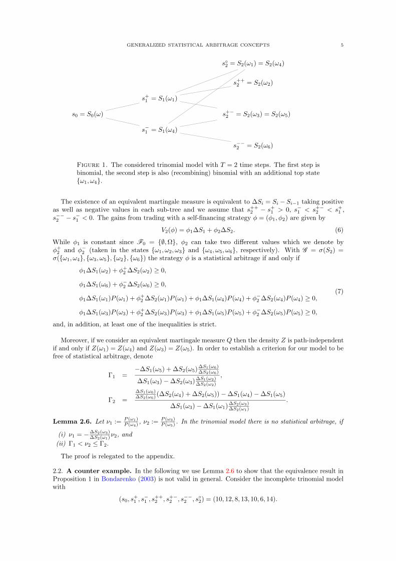
GENERALIZED STATISTICAL ARBITRAGE CONCEPTS 5
s2 = S2(ω1) = S2(ω4)
s++2 = S2(ω2)
s+1 = S1(ω1)
s0 = S0(ω) s+−2 = S2(ω3) = S2(ω5)
s−1 = S1(ω4)
s−−2 = S2(ω6)
Figure 1. The considered trinomial model with T = 2 time steps. The first step isbinomial, the second step is also (recombining) binomial with an additional top stateω1, ω4.
The existence of an equivalent martingale measure is equivalent to ∆Si = Si − Si−1 taking positiveas well as negative values in each sub-tree and we assume that s++
2 − s+1 > 0, s−1 < s+−
2 < s+1 ,
s−−2 − s−1 < 0. The gains from trading with a self-financing strategy φ = (φ1, φ2) are given by
V2(φ) = φ1∆S1 + φ2∆S2. (6)
While φ1 is constant since F0 = ∅,Ω, φ2 can take two different values which we denote byφ+
2 and φ−2 (taken in the states ω1, ω2, ω3 and ω4, ω5, ω6, respectively). With G = σ(S2) =σ(ω1, ω4, ω3, ω5, ω2, ω6) the strategy φ is a statistical arbitrage if and only if
φ1∆S1(ω2) + φ+2 ∆S2(ω2) ≥ 0,
φ1∆S1(ω6) + φ−2 ∆S2(ω6) ≥ 0,
φ1∆S1(ω1)P (ω1) + φ+2 ∆S2(ω1)P (ω1) + φ1∆S1(ω4)P (ω4) + φ−2 ∆S2(ω4)P (ω4) ≥ 0,
φ1∆S1(ω3)P (ω3) + φ+2 ∆S2(ω3)P (ω3) + φ1∆S1(ω5)P (ω5) + φ−2 ∆S2(ω5)P (ω5) ≥ 0,
(7)
and, in addition, at least one of the inequalities is strict.
Moreover, if we consider an equivalent martingale measure Q then the density Z is path-independentif and only if Z(ω1) = Z(ω4) and Z(ω3) = Z(ω5). In order to establish a criterion for our model to befree of statistical arbitrage, denote
Γ1 =−∆S1(ω5) + ∆S2(ω5)∆S1(ω6)
∆S2(ω6)
∆S1(ω3)−∆S2(ω3)∆S1(ω2)∆S2(ω2)
,
Γ2 =
∆S1(ω6)∆S2(ω6) (∆S2(ω4) + ∆S2(ω5))−∆S1(ω4)−∆S1(ω5)
∆S1(ω3)−∆S1(ω1)∆S2(ω3)∆S2(ω1)
.
Lemma 2.6. Let ν1 := P (ω1)P (ω4) , ν2 := P (ω3)
P (ω5) . In the trinomial model there is no statistical arbitrage, if
(i) ν1 = −∆S2(ω3)∆S2(ω1)ν2, and
(ii) Γ1 < ν2 ≤ Γ2.
The proof is relegated to the appendix.
2.2. A counter example. In the following we use Lemma 2.6 to show that the equivalence result inProposition 1 in Bondarenko (2003) is not valid in general. Consider the incomplete trinomial modelwith
(s0, s+1 , s−1 , s
++2 , s+−
2 , s−−2 , s2) = (10, 12, 8, 13, 10, 6, 14).
6 CHRISTIAN REIN, LUDGER RUSCHENDORF, AND THORSTEN SCHMIDT
It is easy to check that the equivalent martingale measures Q specified by q = (Q(ω1), . . . , Q(ω6))are given by the set
Q =q ∈ R6
∣∣∣ q1 = −3
4q2 +
1
4, q3 = −1
4q2 +
1
4, q4 = q6 −
1
4, q5 = −2q6 +
3
4: q2 ∈
(0,
1
3
), q6 ∈
(1
4,
3
8
).
Furthermore, the underlying measure P is specified by the vector p = (P (ω1), . . . , P (ω6)) with
p = (0.15, 0.2, 0.3, 0.05, 0.1, 0.2).
We compute ν1 = p1p4
= 3 and ν2 = p3p5
= 3. Then
Γ2 =
∆S1(ω6)∆S2(ω6) (∆S2(ω4) + ∆S2(ω5))−∆S1(ω4)−∆S1(ω5)
∆S1(ω3)−∆S1(ω1)∆S2(ω3)∆S2(ω1)
= 3 = ν2,
Γ1 =−∆S1(ω5) + ∆S2(ω5)∆S1(ω6)
∆S2(ω6)
∆S1(ω3)−∆S2(ω3)∆S1(ω2)∆S2(ω2)
=2
3< ν2
and
ν1 = −∆S2(ω3)
∆S2(ω1)ν2 = ν2 = 3 =
p1
p4.
According to Lemma 2.6 there is no statistical arbitrage in the stated example. But, on the otherhand, there is no path independent density in this case because if there would be a path independentdensity, i. e. a density Z with Z(ω1) = Z(ω4) and Z(ω3) = Z(ω5), there would exist an equivalentmartingale measure Q fulfilling the conditions
q1
q4=p1
p4= 3 and
q3
q5=p3
p5= 3. (8)
But the only q ≥ 0 fulfilling (8) is q = ( 14 , 0,
14 ,
112 ,
112 ,
13 ) which is not an element of the set Q of
equivalent martingale measures.This example shows that the converse of Theorem 2.4 does not hold in general and therefore,
Proposition 1 in Bondarenko (2003) needs additional assumptions: indeed, we have shown that theredoes not exist a statistical arbitrage and at the same time there is no path-independent density to anequivalent martingale measure.
3. Generalized statistical G -arbitrage strategies
For risk and investment optimization problems it has been shown that conditioning of payoffson the pricing density leads to improved (cost efficient) payoffs (see Burgert and Ruschendorf(2006), Kassberger and Liebmann (2017) and several papers cited therein). In connection with theseimprovement procedures, Kassberger and Liebmann (2017) introduced, in the case where one pricingmeasure Q is specified, the followingg notion of generalized statistical G -arbitrage for a generalstatic payoff X considered as a generalized strategy. Note that in their context no financial marketis specified, Q is any probability measure dominated by P . When a concrete financial market isconsidered, only martingale pricing measures Q will be considered.
Definition 3.1. Let G ⊆ F be a σ-algebra. The set of generalized statistical G -arbitrage-strategieswith respect to a pricing measure Q P is defined as
SA(Q,G ) := X ∈ Lb : EQ[X] ≤ 0, EP [X|G ] ≥ 0 P -a.s. and EP [X] > 0.
The market satisfies NSA(Q,G ), the condition of no generalized statistical G -arbitrage with respect toQ, if
SA(Q,G ) = ∅.
The following result in Kassberger and Liebmann (2017), Proposition 6, characterizes the generalized
NSA(Q,G )-condition by showing that this notion is equivalent to G -measurability of dZ = dQdP .
Proposition 3.2. Let Q ∼ P be an equivalent pricing measure. Then, the no-arbitrage conditionNSA(Q,G )is equivalent to the existence of a G -measurable version of the Radon-Nikodym derivative
Z = dQdP .
GENERALIZED STATISTICAL ARBITRAGE CONCEPTS 7
The proof of this result is achieved by Jensen’s inequality and using as candidate of a generalizedG -arbitrage
X =EP [Z |G ]
Z− 1 ≥ −1. (9)
We aim at studying under which conditions there exist generalized statistical G -arbitrages and todescribe connections between NSA(Q,G ) and NSA(G ). One consequence of Proposition 3.2 is thecharacterization of NSA(G ) for the case of complete market models. Recall that the Radon-Nikodym
derivative Z = dQdP is path-independent, iff Z is σ(ST )-measurable.
A financial market is called complete, if every contingent claim is attainable, i.e. for every F -measurable random variable X bounded from below, we find an admissible self-financing tradingstrategy φ, such that x + VT (φ) = X. This is implied by the assumption that M e = Q: indeed,under this assumption, Theorem 16 in Delbaen and Schachermayer (1995) yields that any X, boundedfrom below, is hedgeable and hence attainable.
Theorem 3.3. Assume that M e = Q. Then NSA(G ) holds if and only if dQdP is G -measurable.
Proof. If Q ∈M e has a G -measurable density dQdP , then, by Theorem 2.4, NSA(G ) holds.
For the converse direction assume that Z is not G -measurable. By Proposition 3.2 it follows thatthere exists a generalized G -arbitrage, i.e. an X ∈ Lb with EQ[X] ≤ 0, EP [X |G ] ≥ 0 and EP [X] > 0.Hence, Theorem 16 in Delbaen and Schachermayer (1995) yields existence of an admissible self-financing trading strategy φ, such that x + VT (φ) = X. Moreover, the superhedging duality, i.e.Theorem 9 in Delbaen and Schachermayer (1995) implies that x = EQ[X] = 0, and hence φ is aG -arbitrage. This is a contradiction and the claim follows.
In particular this result implies that equivalence result (Bondarenko, 2003, Proposition 1) givesa correct characterization of NSA for complete markets. In the following example we give a classof diffusion processes for which, as consequence of Proposition 3.2 and Theorem 3.3, no statisticalG -arbitrage for G = σ(ST ) exists.
Example 3.4 (Statistical arbitrage for diffusions). This example discusses the consequences ofProposition 3.2 and Theorem 3.3 in the case of a diffusion model. Consider a P -Brownian motionB generating the filtration F = FB . Let S be a one-dimensional diffusion process satisfying S0 = s0,s0 ∈ R and
dSt = Stat dt+ Stbt dBt, 0 ≤ t ≤ T, (10)
a and b deterministic and sufficiently integrable. Denote the market price of risk by λt = at/bt. Thenthis model is complete and by Girsanov’s theorem has a unique equivalent local martingale measureQ with Radon-Nikodym derivative
ZT = exp
(−∫ T
0
λ dBt −1
2
∫ T
0
λ2t dt
). (11)
This illustrates that in general, ZT will not be a function of ST . However, if λ = c · b, c ∈ R, then thiscan be possible. Indeed, in this case
ZT = exp
(−c∫ T
0
btdBt −∫ T
0
a2t
2b2tdt
)is a function of ST . We obtain from Theorem 3.3 that there are no statistical arbitrage opportunitieswith respect to G = σ(ST ). This holds in particular when at = a0 and bt = b0, 0 ≤ t ≤ T, i. e. in thecase of constant drift and volatility (the Black-Scholes model). On the other side, the diffusion modelallows for statistical arbitrage in general. A comparable result was obtained in Goncu (2015) whenstudying the concept of statistical arbitrage introduced in Hogan et al. (2004).
The following definition extends the notion of generalized statistical G -arbitrage with respect toa single pricing measure Q in Definition 3.1 to the consideration of a class Q of pricing measures.As a main result of this paper we obtain that in the case Q = M e the corresponding no-arbitragecondition w.r.t. generalized strategies is equivalent to the no-arbitrage condition NSA(G ) w.r.t. tradingstrategies.
8 CHRISTIAN REIN, LUDGER RUSCHENDORF, AND THORSTEN SCHMIDT
Definition 3.5. Let G ⊆ F be a σ-algebra. The set of generalized statistical G -arbitrage-strategiesis defined as
SA(G ) :=X ∈ Lb : sup
Q∈Me
EQ[X] ≤ 0, EP [X|G ] ≥ 0 P -a.s. and EP [X] > 0.
The market satisfies NSA(G ), i.e. no generalized statistical G -arbitrage, if
SA(G ) = ∅.
To establish a connection between statistical G -arbitrage trading strategies and generalized statisticalG -arbitrage strategies, we recall that we assumed use the concept of No Free Lunch with VanishingRisk (NFLVR). Recall that the underliyng process S is assumed to satisfy (NFLVR).
Theorem 3.6. On the financial market given by S it holds that
SA(G ) = SA(G ),
and, in particular,
NSA(G )⇔ NSA(G ).
Proof. We first show that every G -arbitrage strategy is a generalized G -arbitrage strategy: considerφ ∈ SA(G ), i. e. E[VT (φ) |G ] ≥ 0 and E[VT (φ)] > 0. By the superreplication duality, Theorem 9 inDelbaen and Schachermayer (1995), it holds that
supQ∈Me
EQ[VT (φ)] = infx | ∃ admissible φ, x+ VT (φ) ≥ VT (φ).
Choosing φ = φ it follows supQ∈Me EQVT (φ) ≤ 0. Note that in addition, admissibility of φ implies
that VT (φ) is bounded from below and so VT (φ) ∈ SA(G ).For the reverse implication we have, again by the superreplication duality, for X ∈ SA(G ) that
0 ≥ supQ∈Me
EQX = infx ∈ R | ∃ admissible φ, x+ VT (φ) ≥ X.
Since the infimum is finite, Theorem 9 in Delbaen and Schachermayer (1995) yields that it is indeed aminimum. Without loss of generality, we may chose x = 0 and obtain the existence of an admissibledynamic trading strategy φ with X ≤ VT (φ). As X ∈ SA(G ) it holds further that EP [X |G ] ≥ 0, P -a.s., which leads us to
EP [VT (φ) |G ] ≥ EP [X |G ] ≥ 0 P -a.s.
Then, EP [VT (φ)] ≥ EP [X] > 0, such that VT (φ) ∈ SA(G ). So the existence of generalized G -arbitragestrategies is equivalent to the existence of G -arbitrage strategies VT (φ) in SA(G )and the claimfollows.
Using Theorem 2.4, we obtain from Theorem 3.6, that existence of an equivalent local martingalemeasure with a G -measurable density implies even the absence of generalized G -statistical arbitrages.
Corollary 3.7. If there exists Q ∈M e such that dQdP is G -measurable, then NSA(G ) holds.
We remark that the converse of this corollay is still open in the general case.
4. Statistical arbitrage strategies in binomial models
In this section we propose a method to construct trading strategies in binomial models yieldingstatistical arbitrages. These strategies will be used in the Section 5 for the construction of profitabletrading strategies in continuous time by embedding binomial models.
Consider the recombining two-period binomial model: assume that Ω = ω1, . . . , ω4 and T = 2.Let S0 = s0 > 0 and let S1(ω1) = S1(ω2) = s+, and S1(ω3) = S1(ω4) = s− as well as s++ = S2(ω1),s+− = S2(ω2) = S2(ω3), and s−− = S2(ω4). Absence of arbitrage is equivalent to ∆Si, i = 1, 2 takingpositive as well as negative values. We assume without loss of generality that s+ > s0, s
− < s0, and
GENERALIZED STATISTICAL ARBITRAGE CONCEPTS 9
s++ > s+, s− < s+− < s+, and s−− < s−. Gains from trading are again given by (6). Moreover, φ1
is constant and φ2 can take the two values φ+2 , φ
−2 . Then φ = (φ1, φ2) is a statistical arbitrage, iff
φ1∆S1(ω1) + φ+2 ∆S2(ω1) ≥ 0
φ1∆S1(ω4) + φ−2 ∆S2(ω4) ≥ 0
φ1∆S1(ω2)P (ω2) + φ+2 ∆S2(ω2)P (ω2) + φ1∆S1(ω3)P (ω3) + φ−2 ∆S2(ω3)P (ω3) ≥ 0
(12)
and at least one of the inequalities is strict. The density Z is path-independent if and only ifZ(ω2) = Z(ω3). Equations (12) are equivalent to Aφ ≥ 0, φ = (φ1, φ
+2 , φ
−2 )> with
A =
∆S1(ω1) ∆S2(ω1) 0∆S1(ω4) 0 ∆S2(ω4)
q∆S1(ω2) + ∆S1(ω3) q∆S2(ω2) ∆S2(ω3)
, (13)
where q = P (ω2)P (ω3) .
Proposition 4.1. In the recombining two-period binomial model NSA holds if and only if det(A) = 0.Moreover, det(A) = 0 is equivalent to
P (ω2)
P (ω3)=
∆S2(ω1)(∆S1(ω3)∆S2(ω4)−∆S1(ω4)∆S2(ω3))
∆S2(ω4)(∆S1(ω1)∆S2(ω2)−∆S1(ω2)∆S2(ω1))=: q. (14)
.
The proof is relegated to the appendix.
Lemma 4.2. Consider the recombining two-period binomial model with statistical arbitrage. In thismodel, φ = 1
D (ξ1, ξ2, ξ3) with
ξ1 =(q∆S2(ω2) − ∆S2(ω1)
)∆S2(ω4) + ∆S2(ω1)∆S2(ω3),
ξ2 = −(∆S1(ω3) + q∆S1(ω2) − ∆S1(ω1)
)∆S2(ω4) −
(∆S1(ω1) − ∆S1(ω4)
)∆S2(ω3),
ξ3 = −(q∆S1(ω4) − q∆S1(ω1)
)∆S2(ω2) −
(− ∆S1(ω4) + ∆S1(ω3) + q∆S1(ω2)
)∆S2(ω1),
q = P (ω2)P (ω3)
, and
D =(q∆S1(ω1)∆S2(ω2) +
(− ∆S1(ω3) − q∆S1(ω2)
)∆S2(ω1)
)∆S2(ω4) + ∆S1(ω4)∆S2(ω1)∆S2(ω3)
is a statistical arbitrage.
Proof. If P (ω2)P (ω3) 6= q we have statistical arbitrage according to Proposition 4.1 and that the determinant
of the matrix A in (13) is not equal to zero. In this case the matrix A is invertible. Hence, φ = A−11
is a statistical arbitrage and it is easily verified that φ = 1D (ξ1, ξ2, ξ3).
Remark 4.3 (Risk of statistical arbitrages). The word arbitrage might be misleading on the riskinessof statistical arbitrages, because in the classical sense, an arbitrage is a strategy without risk. Thisis of course not the case for statistical arbitrages (or the following generalizations of this concept).Since we consider arbitrage-free markets, all gains come with a certain risk and, higher profits areassociated with higher risk. This is confirmed by our simulation results in the following section.
As a simple example consider the case of the binomial model where ∆iS(ωj) ∈ 5,−5, i.e. thestock either rises by 5 or falls by 5. In addition, assume that q = P (ω2)/P (ω3) = 1.2. Then, usingEquation (13) it is not difficult to compute φ = A−11 = (1.6,−1.4,−1.8)>. From this strategy weobtain that the gains at time 2, given by
G2(ω) = φ1(ω)∆S1(ω) + φ2(ω)∆S2(ω),
yield G2(ω1) = G2(ω4) = 1, corresponding to (12). In addition, we obtain that G2(ω2) = 15 andG2(ω3) = −17. If we assume that P (ω2) = 0.3 we obtain that the average expected gain on ω2, ω3computes to
P (ω2)G2(ω2) + P (ω3)G3(ω3) = 0.3 · 15 + 0.25 · (−17) = 0.25 ≥ 0, (15)
such that the strategy is indeed a statistical arbitrage. While the (average) gains in the threerelevant scenarios are 1, 0.25, 1, the possible loss in scenario ω3 is equal to −17, which is attained withprobability 0.25, clearly pointing out the riskiness of the strategy.
10 CHRISTIAN REIN, LUDGER RUSCHENDORF, AND THORSTEN SCHMIDT
To exploit the averaging property of statistical arbitrage, we keep repeating this strategy until wefirst record a positive P&L. These considerations show clearly, that a risk analysis of the implementedstrategy is important.
5. Profitable strategies
Up to now we saw conditions and examples of statistical arbitrages in a variety of models. Here weare considering several classes of simple statistical arbitrage strategies for several classes of σ-fields G .While these strategies are useful and easy to apply for general stochastic models we investigate themon the Black-Scholes model which allows to explicitly check by analytic formulas for the involvedstopping times the corresponding (no-)arbitrage condition. For more general models this has to bechecked numerically.
The Black-Scholes model is, according to Example 3.4, free of statistical arbitrage. For some choicesof G , however, G -arbitrage strategies may exist in the Black-Scholes model. We show in the followinghow to construct dynamic trading strategies allowing statistical G -arbitrage for various choices of G .To this end, assume that S is a geometric Brownian motion, i.e. the unique strong solution of thestochastic differential equation
dSt = µSt dt+ σSt dBt, 0 ≤ t ≤ T (16)
where B is a P -Brownian motion and σ > 0. In the simulation we will first chose µ = 0.1241,σ = 0.0837, S0 = 2186 according to estimated drift and volatility from the S&P 500 (September 2016to August 2017), and later consider small variations.
Motivated by our findings in Section 2.1, we begin by embedding binomial trading strategies intothe diffusion setting by considering two limits (up / down) and taking actions at the first times theselimits are reached. In Section 5.3 we will introduce some related follow-the-trend strategies.
5.1. Embedded binomial trading strategies. We introduce a recombination of several two-stepbinomial models embedded in the continuous-time model as long as the final time T is reached. Weconsider the σ-fields generated by the stopping times when the final states of each of the binomialmodels are reached (or the trivial σ-field otherwise).
As we repeatedly consider embedded binomial models it makes sense to consider the outcome of thetrading strategy on average conditional on the final states of each binomial model, i.e. by averagingthe outcome over many repeated applications of the trading strategy and hence we get in this way anestimate for the statistical arbitrage in the whole time interval [0, T ].
Let i denote the current step of our iteration and consider a multiplicative step size c > 0. Weinitialize at time t00 = 0. Otherwise consider the initial time of our next iteration given by the timewhen the last repetition finished and denote this time by ti0 and the according level by si0 = Sti0 . Thenwe define the following two stopping times corresponding to the first and second period of our binomialmodel by
ti1 = inft ∈ [ti0, T ] |St ∈ si0(1− c), si0(1 + c)
(17)
and
ti2 = inft ∈ (ti1, T ] |St ∈ si0(1− 2c), si0, s
i0(1 + 2c)
, (18)
with the convention that inf ∅ = T . This induces a sequence of σ-fields
G i := σ(Sti2).
Since S is continuous, this scheme allows to embed repeated binomial models Sti0 , Sti1 , Sti2 , i =1, 2, . . . , N into continuous time with a random number N of repetitions. The proposed tradingstrategy then is to execute successively the statistical arbitrage strategy for binomial models computedin Lemma 4.2 at the stopping times ti0, t
i1, t
i2. At ti2 the position will be cleared and we start the
procedure afresh by letting ti+10 = ti2. Generally, we assume that the time horizon T is sufficiently
large such that the (typically small) levels si0(1− 2c), . . . , si0(1 + 2c) are reached at least once.Using the independent increments property of the Black-Scholes model we find that the achieved
repeated statistical G i-arbitrage strategies constitute a statistical G -arbitrage with respect to
G = σ(St12 , St22 , . . . , StN2
).
GENERALIZED STATISTICAL ARBITRAGE CONCEPTS 11
gain p.a. median VaR(0.95) gain/trade losses (mean) ∅ N max. N
33.4 206 5,320 8.74 0.133 -628 3.82 24
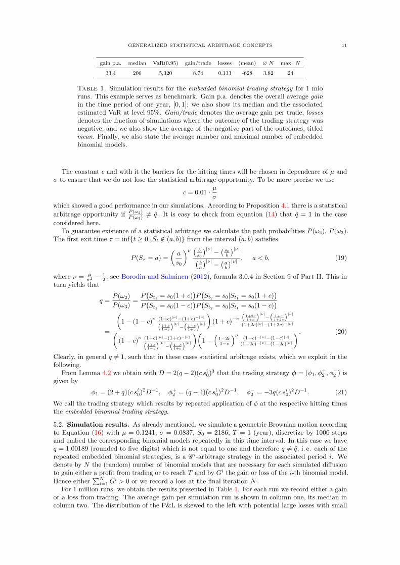
Table 1. Simulation results for the embedded binomial trading strategy for 1 mioruns. This example serves as benchmark. Gain p.a. denotes the overall average gainin the time period of one year, [0, 1]; we also show its median and the associatedestimated VaR at level 95%. Gain/trade denotes the average gain per trade, lossesdenotes the fraction of simulations where the outcome of the trading strategy wasnegative, and we also show the average of the negative part of the outcomes, titledmean. Finally, we also state the average number and maximal number of embeddedbinomial models.
The constant c and with it the barriers for the hitting times will be chosen in dependence of µ andσ to ensure that we do not lose the statistical arbitrage opportunity. To be more precise we use
c = 0.01 · µσ
which showed a good performance in our simulations. According to Proposition 4.1 there is a statistical
arbitrage opportunity if P (ω2)P (ω3) 6= q. It is easy to check from equation (14) that q = 1 in the case
considered here.To guarantee existence of a statistical arbitrage we calculate the path probabilities P (ω2), P (ω3).
The first exit time τ = inft ≥ 0 |St /∈ (a, b) from the interval (a, b) satisfies
P (Sτ = a) =
(a
s0
)ν ( bs0
)|ν| − ( s0b )|ν|(ba
)|ν| − (ab )|ν| , a < b, (19)
where ν = µσ2 − 1
2 , see Borodin and Salminen (2012), formula 3.0.4 in Section 9 of Part II. This inturn yields that
q =P (ω2)
P (ω3)=P(St1 = s0(1 + c)
)P(St2 = s0|St1 = s0(1 + c)
)P(St1 = s0(1− c)
)P(St2 = s0|St1 = s0(1− c)
)
=
(1− (1− c)ν (1+c)|ν|−(1+c)−|ν|(
1+c1−c
)|ν|−(
1−c1+c
)|ν|) (1 + c)−ν(
1+2c1+c
)|ν|−(
1+c1+2c
)|ν|(1+2c)|ν|−(1+2c)−|ν|(
(1− c)ν (1+c)|ν|−(1+c)−|ν|(1+c1−c
)|ν|−(
1−c1+c
)|ν|)(1−(
1−2c1−c
)ν(1−c)−|ν|−(1−c)|ν|
(1−2c)−|ν|−(1−2c)|ν|
) . (20)
Clearly, in general q 6= 1, such that in these cases statistical arbitrage exists, which we exploit in thefollowing.
From Lemma 4.2 we obtain with D = 2(q − 2)(c si0)3 that the trading strategy φ = (φ1, φ+2 , φ
−2 ) is
given by
φ1 = (2 + q)(c si0)2D−1, φ+2 = (q − 4)(c si0)2D−1, φ−2 = −3q(c si0)2D−1. (21)
We call the trading strategy which results by repeated application of φ at the respective hitting timesthe embedded binomial trading strategy.
5.2. Simulation results. As already mentioned, we simulate a geometric Brownian motion accordingto Equation (16) with µ = 0.1241, σ = 0.0837, S0 = 2186, T = 1 (year), discretize by 1000 stepsand embed the corresponding binomial models repeatedly in this time interval. In this case we haveq = 1.00189 (rounded to five digits) which is not equal to one and therefore q 6= q, i. e. each of therepeated embedded binomial strategies, is a G i-arbitrage strategy in the associated period i. Wedenote by N the (random) number of binomial models that are necessary for each simulated diffusionto gain either a profit from trading or to reach T and by Gi the gain or loss of the i-th binomial model.
Hence either∑Ni=1G
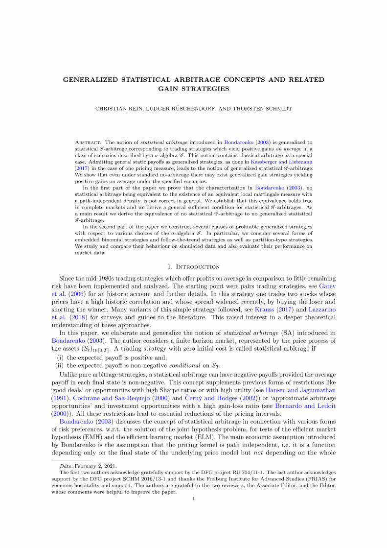
i > 0 or we record a loss at the final iteration N .For 1 million runs, we obtain the results presented in Table 1. For each run we record either a gain
or a loss from trading. The average gain per simulation run is shown in column one, its median incolumn two. The distribution of the P&L is skewed to the left with potential large losses with small
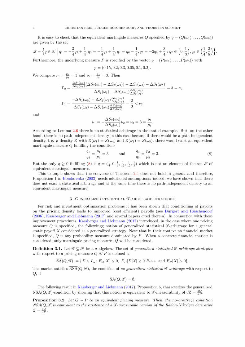
12 CHRISTIAN REIN, LUDGER RUSCHENDORF, AND THORSTEN SCHMIDT
−10000 −8000 −6000 −4000 −2000 0 2000
0e+0
01e
+05
2e+0
53e
+05
4e+0
55e
+05
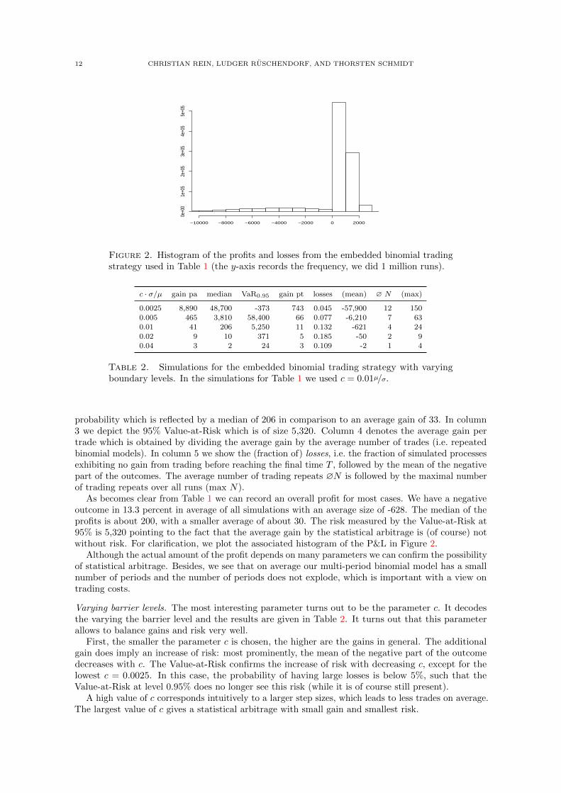
Figure 2. Histogram of the profits and losses from the embedded binomial tradingstrategy used in Table 1 (the y-axis records the frequency, we did 1 million runs).
c · σ/µ gain pa median VaR0.95 gain pt losses (mean) ∅ N (max)
0.0025 8,890 48,700 -373 743 0.045 -57,900 12 1500.005 465 3,810 58,400 66 0.077 -6,210 7 63
0.01 41 206 5,250 11 0.132 -621 4 24
0.02 9 10 371 5 0.185 -50 2 90.04 3 2 24 3 0.109 -2 1 4
Table 2. Simulations for the embedded binomial trading strategy with varyingboundary levels. In the simulations for Table 1 we used c = 0.01µ/σ.
probability which is reflected by a median of 206 in comparison to an average gain of 33. In column3 we depict the 95% Value-at-Risk which is of size 5,320. Column 4 denotes the average gain pertrade which is obtained by dividing the average gain by the average number of trades (i.e. repeatedbinomial models). In column 5 we show the (fraction of) losses, i.e. the fraction of simulated processesexhibiting no gain from trading before reaching the final time T , followed by the mean of the negativepart of the outcomes. The average number of trading repeats ∅N is followed by the maximal numberof trading repeats over all runs (max N).
As becomes clear from Table 1 we can record an overall profit for most cases. We have a negativeoutcome in 13.3 percent in average of all simulations with an average size of -628. The median of theprofits is about 200, with a smaller average of about 30. The risk measured by the Value-at-Risk at95% is 5,320 pointing to the fact that the average gain by the statistical arbitrage is (of course) notwithout risk. For clarification, we plot the associated histogram of the P&L in Figure 2.
Although the actual amount of the profit depends on many parameters we can confirm the possibilityof statistical arbitrage. Besides, we see that on average our multi-period binomial model has a smallnumber of periods and the number of periods does not explode, which is important with a view ontrading costs.
Varying barrier levels. The most interesting parameter turns out to be the parameter c. It decodesthe varying the barrier level and the results are given in Table 2. It turns out that this parameterallows to balance gains and risk very well.
First, the smaller the parameter c is chosen, the higher are the gains in general. The additionalgain does imply an increase of risk: most prominently, the mean of the negative part of the outcomedecreases with c. The Value-at-Risk confirms the increase of risk with decreasing c, except for thelowest c = 0.0025. In this case, the probability of having large losses is below 5%, such that theValue-at-Risk at level 0.95% does no longer see this risk (while it is of course still present).
A high value of c corresponds intuitively to a larger step sizes, which leads to less trades on average.The largest value of c gives a statistical arbitrage with small gain and smallest risk.
GENERALIZED STATISTICAL ARBITRAGE CONCEPTS 13
η gain pa median VaR0.95 gain pt losses (mean) ∅ N (max)
0.50 170 4,360 94,500 36 0.13 -11,000 5 30
0.75 109 1,730 38,100 23 0.13 -4,400 5 30
1.00 64 913 20,400 14 0.12 -2,340 5 301.25 77 561 12,400 17 0.12 -1,400 5 30
2.00 42 197 4,430 9 0.11 -490 4 31
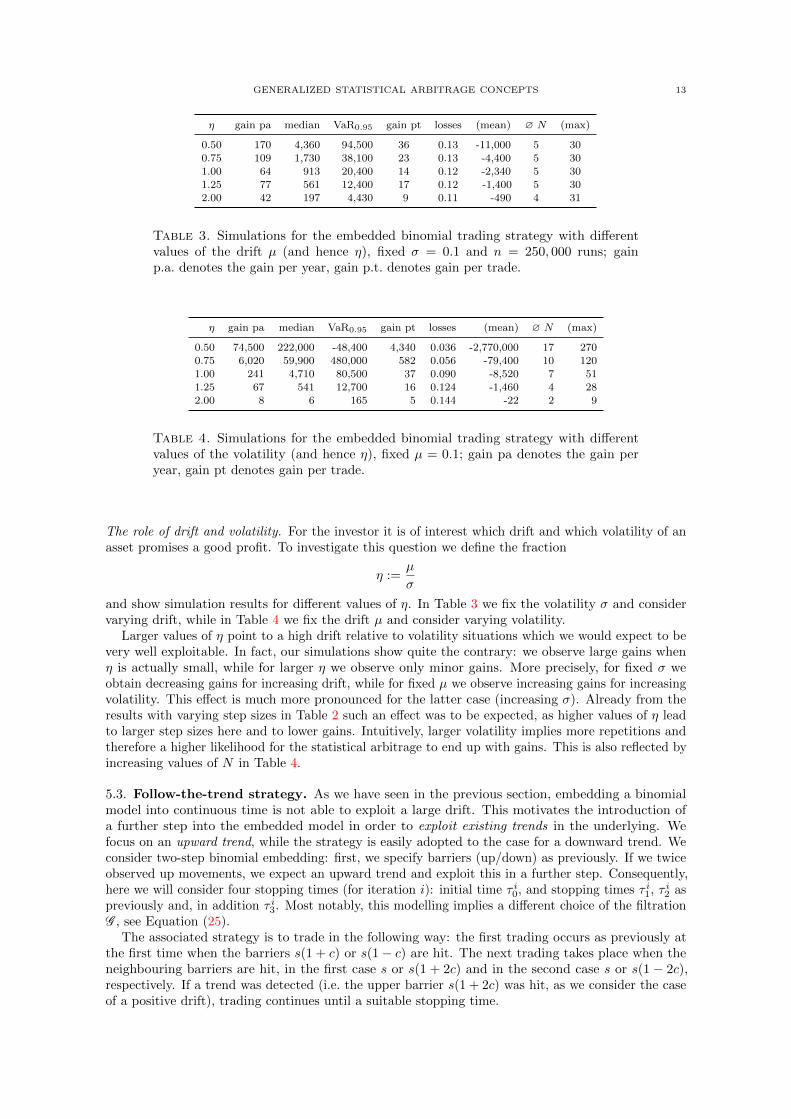
Table 3. Simulations for the embedded binomial trading strategy with differentvalues of the drift µ (and hence η), fixed σ = 0.1 and n = 250, 000 runs; gainp.a. denotes the gain per year, gain p.t. denotes gain per trade.
η gain pa median VaR0.95 gain pt losses (mean) ∅ N (max)
0.50 74,500 222,000 -48,400 4,340 0.036 -2,770,000 17 2700.75 6,020 59,900 480,000 582 0.056 -79,400 10 120
1.00 241 4,710 80,500 37 0.090 -8,520 7 51
1.25 67 541 12,700 16 0.124 -1,460 4 282.00 8 6 165 5 0.144 -22 2 9
Table 4. Simulations for the embedded binomial trading strategy with differentvalues of the volatility (and hence η), fixed µ = 0.1; gain pa denotes the gain peryear, gain pt denotes gain per trade.
The role of drift and volatility. For the investor it is of interest which drift and which volatility of anasset promises a good profit. To investigate this question we define the fraction
η :=µ
σ
and show simulation results for different values of η. In Table 3 we fix the volatility σ and considervarying drift, while in Table 4 we fix the drift µ and consider varying volatility.
Larger values of η point to a high drift relative to volatility situations which we would expect to bevery well exploitable. In fact, our simulations show quite the contrary: we observe large gains whenη is actually small, while for larger η we observe only minor gains. More precisely, for fixed σ weobtain decreasing gains for increasing drift, while for fixed µ we observe increasing gains for increasingvolatility. This effect is much more pronounced for the latter case (increasing σ). Already from theresults with varying step sizes in Table 2 such an effect was to be expected, as higher values of η leadto larger step sizes here and to lower gains. Intuitively, larger volatility implies more repetitions andtherefore a higher likelihood for the statistical arbitrage to end up with gains. This is also reflected byincreasing values of N in Table 4.
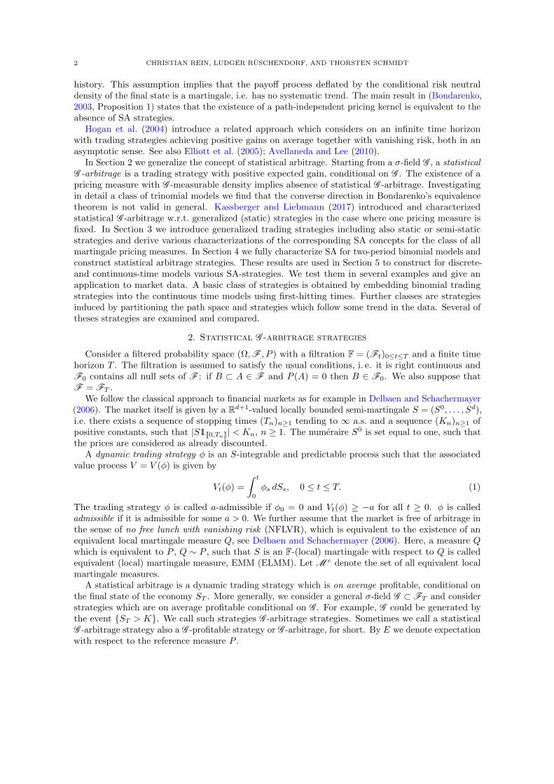
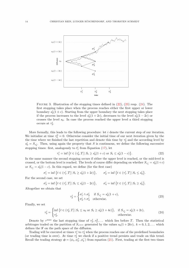
5.3. Follow-the-trend strategy. As we have seen in the previous section, embedding a binomialmodel into continuous time is not able to exploit a large drift. This motivates the introduction ofa further step into the embedded model in order to exploit existing trends in the underlying. Wefocus on an upward trend, while the strategy is easily adopted to the case for a downward trend. Weconsider two-step binomial embedding: first, we specify barriers (up/down) as previously. If we twiceobserved up movements, we expect an upward trend and exploit this in a further step. Consequently,here we will consider four stopping times (for iteration i): initial time τ i0, and stopping times τ i1, τ i2 aspreviously and, in addition τ i3. Most notably, this modelling implies a different choice of the filtrationG , see Equation (25).
The associated strategy is to trade in the following way: the first trading occurs as previously atthe first time when the barriers s(1 + c) or s(1− c) are hit. The next trading takes place when theneighbouring barriers are hit, in the first case s or s(1 + 2c) and in the second case s or s(1 − 2c),respectively. If a trend was detected (i.e. the upper barrier s(1 + 2c) was hit, as we consider the caseof a positive drift), trading continues until a suitable stopping time.
14 CHRISTIAN REIN, LUDGER RUSCHENDORF, AND THORSTEN SCHMIDT
Index
Diffu
sio
n
τ i1
σi1
σi2
σi3
τ i2 τ i3
s0
s0(1 − 2c)
s0(1 − 4c)
s0(1 + 2c)
s0(1 + 4c)
Figure 3. Illustration of the stopping times defined in (22), (23) resp. (24). Thefirst stopping takes place when the process reaches either the first upper or lowerboundary si0(1± c). Starting from the upper boundary the next stopping takes placeif the process increases to the level si0(1 + 2c), decreases to the level si0(1 − 2c) orcrosses the level s0. In case the process reached the upper level a third stoppingoccurs at τ i3.
More formally, this leads to the following procedure: let i denote the current step of our iteration.We initialize at time τ0
0 = 0. Otherwise consider the initial time of our next iteration given by thethe time where we finished the last repetition and denote this time by τ i0 and the according level bysi0 = Sτ i0 . Then, using again the property that S is continuous, we define the following successive
stopping times: first, analogously to ti1 from Equation (17), let
τ i1 = inft ∈ (τ i0, T ] |St ≥ si0(1 + c) or St ≤ si0(1− c)
. (22)
In the same manner the second stopping occurs if either the upper level is reached, or the mid-level iscrossed, or the bottom level is reached. The levels of course differ depending on whether Sτ i1 = si0(1+c)
or Sτ i1 = si0(1− c). In this regard, we define (for the first case)
σi1 = inft ∈ (τ i1, T ] |St ≥ si0(1 + 2c)
, σi2 = inf
t ∈ (τ i1, T ] |St ≤ si0
.
For the second case, we set
σi3 = inft ∈ (τ i1, T ] |St ≤ si0(1− 2c)
, σi4 = inf
t ∈ (τ i1, T ] |St ≥ si0
.
Altogether we obtain that
τ i2 =
σi1 ∧ σi2 if Sτ i1 = si0(1 + c),
σi3 ∧ σi4 otherwise.(23)
Finally, we set
τ i3 =
inft ∈ (τ i2, T ] |St ≤ s0 or St ≥ si0(1 + 4c)
, if Sτ i2 = si0(1 + 2c),
τ i2, otherwise.(24)
Denote by τmax the last stopping time of τ13 , τ
23 , . . . which lies before T . Then the statistical
arbitrages traded on the partition of Sτmax generated by the values s0(1 + 2kc), k = 0, 1, 2, . . . whichdefines the G on the path space of the diffusion.
Trading will be executed at times τ i1 to τ i3 when the process reaches one of the predefined boundaries(or trading time is over). At time τ i2 we check if a positive trend persists and trade on this trend.Recall the trading strategy φ = (φ1, φ
+2 , φ
−2 ) from equation (21). First, trading at the first two times
GENERALIZED STATISTICAL ARBITRAGE CONCEPTS 15
S3(ω1) = s+++
S2(ω1, ω5)
S1(ω1, ω2, ω5)
S0 = s S2(ω2, ω3) = s+− S3(ω5) = s++−
S1(ω3, ω4)
S2(ω4) = s−−
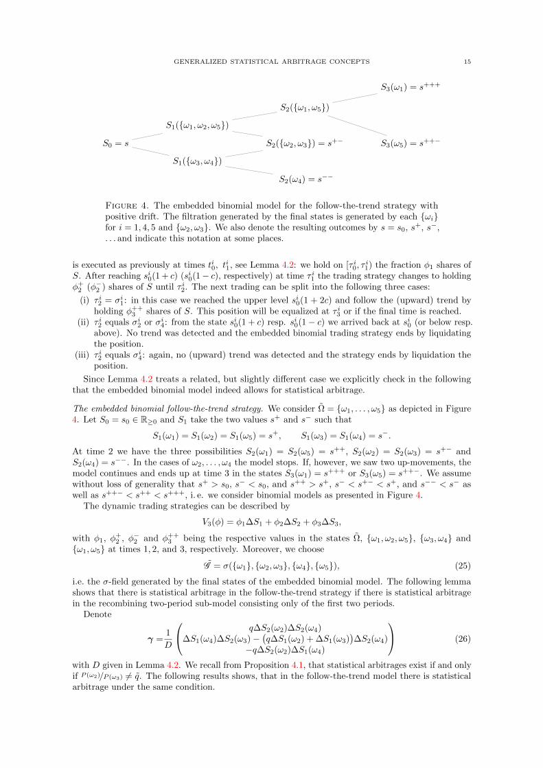
Figure 4. The embedded binomial model for the follow-the-trend strategy withpositive drift. The filtration generated by the final states is generated by each ωifor i = 1, 4, 5 and ω2, ω3. We also denote the resulting outcomes by s = s0, s+, s−,. . . and indicate this notation at some places.
is executed as previously at times ti0, ti1, see Lemma 4.2: we hold on [τ i0, τ
i1) the fraction φ1 shares of
S. After reaching si0(1 + c) (si0(1− c), respectively) at time τ i1 the trading strategy changes to holdingφ+
2 (φ−2 ) shares of S until τ i2. The next trading can be split into the following three cases:
(i) τ i2 = σi1: in this case we reached the upper level si0(1 + 2c) and follow the (upward) trend byholding φ++
3 shares of S. This position will be equalized at τ i3 or if the final time is reached.(ii) τ i2 equals σi2 or σi4: from the state si0(1 + c) resp. si0(1− c) we arrived back at si0 (or below resp.
above). No trend was detected and the embedded binomial trading strategy ends by liquidatingthe position.
(iii) τ i2 equals σi4: again, no (upward) trend was detected and the strategy ends by liquidation theposition.
Since Lemma 4.2 treats a related, but slightly different case we explicitly check in the followingthat the embedded binomial model indeed allows for statistical arbitrage.
The embedded binomial follow-the-trend strategy. We consider Ω = ω1, . . . , ω5 as depicted in Figure4. Let S0 = s0 ∈ R≥0 and S1 take the two values s+ and s− such that
S1(ω1) = S1(ω2) = S1(ω5) = s+, S1(ω3) = S1(ω4) = s−.
At time 2 we have the three possibilities S2(ω1) = S2(ω5) = s++, S2(ω2) = S2(ω3) = s+− andS2(ω4) = s−−. In the cases of ω2, . . . , ω4 the model stops. If, however, we saw two up-movements, themodel continues and ends up at time 3 in the states S3(ω1) = s+++ or S3(ω5) = s++−. We assumewithout loss of generality that s+ > s0, s
− < s0, and s++ > s+, s− < s+− < s+, and s−− < s− aswell as s++− < s++ < s+++, i. e. we consider binomial models as presented in Figure 4.
The dynamic trading strategies can be described by
V3(φ) = φ1∆S1 + φ2∆S2 + φ3∆S3,
with φ1, φ+2 , φ−2 and φ++
3 being the respective values in the states Ω, ω1, ω2, ω5, ω3, ω4 andω1, ω5 at times 1, 2, and 3, respectively. Moreover, we choose
G = σ(ω1, ω2, ω3, ω4, ω5), (25)
i.e. the σ-field generated by the final states of the embedded binomial model. The following lemmashows that there is statistical arbitrage in the follow-the-trend strategy if there is statistical arbitragein the recombining two-period sub-model consisting only of the first two periods.
Denote
γ =1
D
q∆S2(ω2)∆S2(ω4)∆S1(ω4)∆S2(ω3)−
(q∆S1(ω2) + ∆S1(ω3)
)∆S2(ω4)
−q∆S2(ω2)∆S1(ω4)
(26)
with D given in Lemma 4.2. We recall from Proposition 4.1, that statistical arbitrages exist if and onlyif P (ω2)/P (ω3) 6= q. The following results shows, that in the follow-the-trend model there is statisticalarbitrage under the same condition.
16 CHRISTIAN REIN, LUDGER RUSCHENDORF, AND THORSTEN SCHMIDT
gain pa mean VaR0.95 gain pt losses (mean) ∅ N (max)
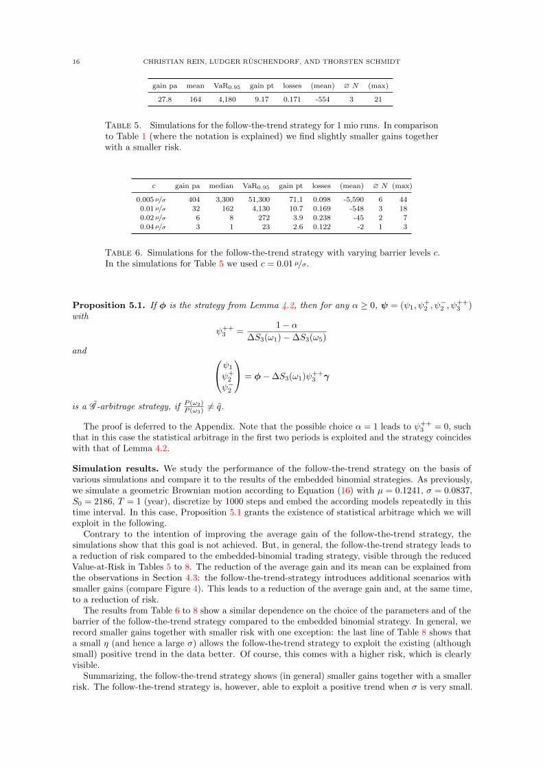
27.8 164 4,180 9.17 0.171 -554 3 21
Table 5. Simulations for the follow-the-trend strategy for 1 mio runs. In comparisonto Table 1 (where the notation is explained) we find slightly smaller gains togetherwith a smaller risk.
c gain pa median VaR0.95 gain pt losses (mean) ∅ N (max)
0.005 µ/σ 404 3,300 51,300 71.1 0.098 -5,590 6 44
0.01 µ/σ 32 162 4,130 10.7 0.169 -548 3 18
0.02 µ/σ 6 8 272 3.9 0.238 -45 2 70.04 µ/σ 3 1 23 2.6 0.122 -2 1 3
Table 6. Simulations for the follow-the-trend strategy with varying barrier levels c.In the simulations for Table 5 we used c = 0.01 µ/σ.
Proposition 5.1. If φ is the strategy from Lemma 4.2, then for any α ≥ 0, ψ = (ψ1, ψ+2 , ψ
−2 , ψ
++3 )
with
ψ++3 =
1− α∆S3(ω1)−∆S3(ω5)
and ψ1
ψ+2
ψ−2
= φ−∆S3(ω1)ψ++3 γ
is a G -arbitrage strategy, if P (ω2)P (ω3) 6= q.
The proof is deferred to the Appendix. Note that the possible choice α = 1 leads to ψ++3 = 0, such
that in this case the statistical arbitrage in the first two periods is exploited and the strategy coincideswith that of Lemma 4.2.
Simulation results. We study the performance of the follow-the-trend strategy on the basis ofvarious simulations and compare it to the results of the embedded binomial strategies. As previously,we simulate a geometric Brownian motion according to Equation (16) with µ = 0.1241, σ = 0.0837,S0 = 2186, T = 1 (year), discretize by 1000 steps and embed the according models repeatedly in thistime interval. In this case, Proposition 5.1 grants the existence of statistical arbitrage which we willexploit in the following.
Contrary to the intention of improving the average gain of the follow-the-trend strategy, thesimulations show that this goal is not achieved. But, in general, the follow-the-trend strategy leads toa reduction of risk compared to the embedded-binomial trading strategy, visible through the reducedValue-at-Risk in Tables 5 to 8. The reduction of the average gain and its mean can be explained fromthe observations in Section 4.3: the follow-the-trend-strategy introduces additional scenarios withsmaller gains (compare Figure 4). This leads to a reduction of the average gain and, at the same time,to a reduction of risk.
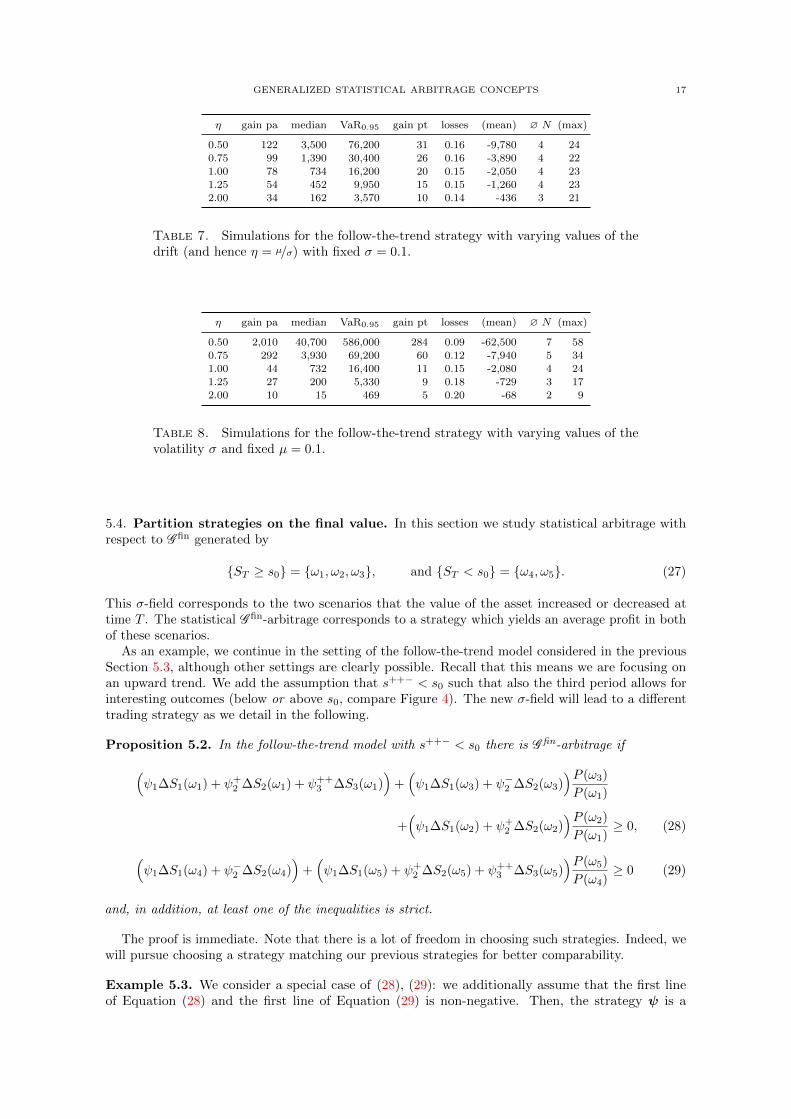
The results from Table 6 to 8 show a similar dependence on the choice of the parameters and of thebarrier of the follow-the-trend strategy compared to the embedded binomial strategy. In general, werecord smaller gains together with smaller risk with one exception: the last line of Table 8 shows thata small η (and hence a large σ) allows the follow-the-trend strategy to exploit the existing (althoughsmall) positive trend in the data better. Of course, this comes with a higher risk, which is clearlyvisible.
Summarizing, the follow-the-trend strategy shows (in general) smaller gains together with a smallerrisk. The follow-the-trend strategy is, however, able to exploit a positive trend when σ is very small.
GENERALIZED STATISTICAL ARBITRAGE CONCEPTS 17
η gain pa median VaR0.95 gain pt losses (mean) ∅ N (max)
0.50 122 3,500 76,200 31 0.16 -9,780 4 24
0.75 99 1,390 30,400 26 0.16 -3,890 4 22
1.00 78 734 16,200 20 0.15 -2,050 4 231.25 54 452 9,950 15 0.15 -1,260 4 23
2.00 34 162 3,570 10 0.14 -436 3 21
Table 7. Simulations for the follow-the-trend strategy with varying values of thedrift (and hence η = µ/σ) with fixed σ = 0.1.
η gain pa median VaR0.95 gain pt losses (mean) ∅ N (max)
0.50 2,010 40,700 586,000 284 0.09 -62,500 7 58
0.75 292 3,930 69,200 60 0.12 -7,940 5 341.00 44 732 16,400 11 0.15 -2,080 4 24
1.25 27 200 5,330 9 0.18 -729 3 17
2.00 10 15 469 5 0.20 -68 2 9
Table 8. Simulations for the follow-the-trend strategy with varying values of thevolatility σ and fixed µ = 0.1.
5.4. Partition strategies on the final value. In this section we study statistical arbitrage withrespect to G fin generated by
ST ≥ s0 = ω1, ω2, ω3, and ST < s0 = ω4, ω5. (27)
This σ-field corresponds to the two scenarios that the value of the asset increased or decreased attime T . The statistical G fin-arbitrage corresponds to a strategy which yields an average profit in bothof these scenarios.
As an example, we continue in the setting of the follow-the-trend model considered in the previousSection 5.3, although other settings are clearly possible. Recall that this means we are focusing onan upward trend. We add the assumption that s++− < s0 such that also the third period allows forinteresting outcomes (below or above s0, compare Figure 4). The new σ-field will lead to a differenttrading strategy as we detail in the following.
Proposition 5.2. In the follow-the-trend model with s++− < s0 there is G fin-arbitrage if(ψ1∆S1(ω1) + ψ+
2 ∆S2(ω1) + ψ++3 ∆S3(ω1)
)+(ψ1∆S1(ω3) + ψ−2 ∆S2(ω3)
)P (ω3)
P (ω1)
+(ψ1∆S1(ω2) + ψ+
2 ∆S2(ω2))P (ω2)
P (ω1)≥ 0, (28)
(ψ1∆S1(ω4) + ψ−2 ∆S2(ω4)
)+(ψ1∆S1(ω5) + ψ+
2 ∆S2(ω5) + ψ++3 ∆S3(ω5)
)P (ω5)
P (ω4)≥ 0 (29)
and, in addition, at least one of the inequalities is strict.
The proof is immediate. Note that there is a lot of freedom in choosing such strategies. Indeed, wewill pursue choosing a strategy matching our previous strategies for better comparability.
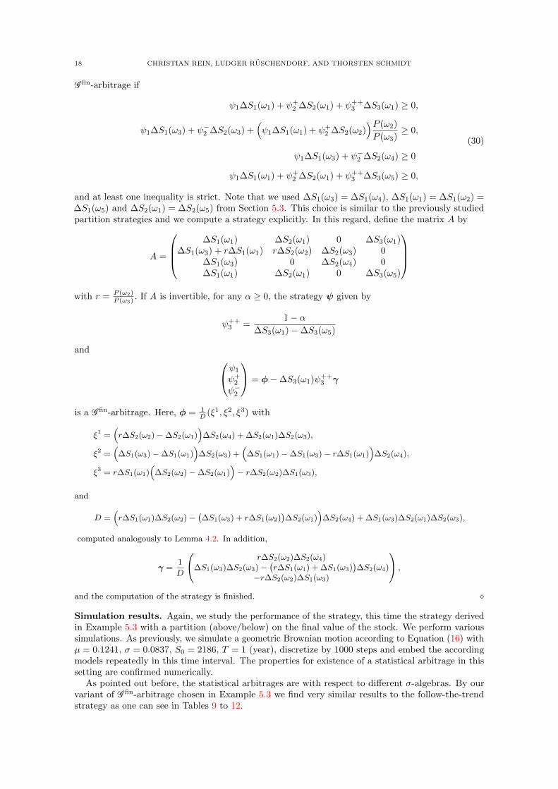
Example 5.3. We consider a special case of (28), (29): we additionally assume that the first lineof Equation (28) and the first line of Equation (29) is non-negative. Then, the strategy ψ is a
18 CHRISTIAN REIN, LUDGER RUSCHENDORF, AND THORSTEN SCHMIDT
G fin-arbitrage if
ψ1∆S1(ω1) + ψ+2 ∆S2(ω1) + ψ++
3 ∆S3(ω1) ≥ 0,
ψ1∆S1(ω3) + ψ−2 ∆S2(ω3) +(ψ1∆S1(ω1) + ψ+
2 ∆S2(ω2))P (ω2)
P (ω3)≥ 0,
ψ1∆S1(ω3) + ψ−2 ∆S2(ω4) ≥ 0
ψ1∆S1(ω1) + ψ+2 ∆S2(ω1) + ψ++
3 ∆S3(ω5) ≥ 0,
(30)
and at least one inequality is strict. Note that we used ∆S1(ω3) = ∆S1(ω4), ∆S1(ω1) = ∆S1(ω2) =∆S1(ω5) and ∆S2(ω1) = ∆S2(ω5) from Section 5.3. This choice is similar to the previously studiedpartition strategies and we compute a strategy explicitly. In this regard, define the matrix A by
A =
∆S1(ω1) ∆S2(ω1) 0 ∆S3(ω1)
∆S1(ω3) + r∆S1(ω1) r∆S2(ω2) ∆S2(ω3) 0∆S1(ω3) 0 ∆S2(ω4) 0∆S1(ω1) ∆S2(ω1) 0 ∆S3(ω5)
with r = P (ω2)
P (ω3) . If A is invertible, for any α ≥ 0, the strategy ψ given by
ψ++3 =
1− α∆S3(ω1)−∆S3(ω5)
and ψ1
ψ+2
ψ−2
= φ−∆S3(ω1)ψ++3 γ
is a G fin-arbitrage. Here, φ = 1D (ξ1, ξ2, ξ3) with
ξ1 =(r∆S2(ω2) − ∆S2(ω1)
)∆S2(ω4) + ∆S2(ω1)∆S2(ω3),
ξ2 =(
∆S1(ω3) − ∆S1(ω1))
∆S2(ω3) +(
∆S1(ω1) − ∆S1(ω3) − r∆S1(ω1))
∆S2(ω4),
ξ3 = r∆S1(ω1)(
∆S2(ω2) − ∆S2(ω1))− r∆S2(ω2)∆S1(ω3),
and
D =(r∆S1(ω1)∆S2(ω2) −
(∆S1(ω3) + r∆S1(ω2)
)∆S2(ω1)
)∆S2(ω4) + ∆S1(ω3)∆S2(ω1)∆S2(ω3),
computed analogously to Lemma 4.2. In addition,
γ =1
D
r∆S2(ω2)∆S2(ω4)∆S1(ω3)∆S2(ω3) −
(r∆S1(ω1) + ∆S1(ω3)
)∆S2(ω4)
−r∆S2(ω2)∆S1(ω3)
,
and the computation of the strategy is finished.
Simulation results. Again, we study the performance of the strategy, this time the strategy derivedin Example 5.3 with a partition (above/below) on the final value of the stock. We perform varioussimulations. As previously, we simulate a geometric Brownian motion according to Equation (16) withµ = 0.1241, σ = 0.0837, S0 = 2186, T = 1 (year), discretize by 1000 steps and embed the accordingmodels repeatedly in this time interval. The properties for existence of a statistical arbitrage in thissetting are confirmed numerically.
As pointed out before, the statistical arbitrages are with respect to different σ-algebras. By ourvariant of G fin-arbitrage chosen in Example 5.3 we find very similar results to the follow-the-trendstrategy as one can see in Tables 9 to 12.
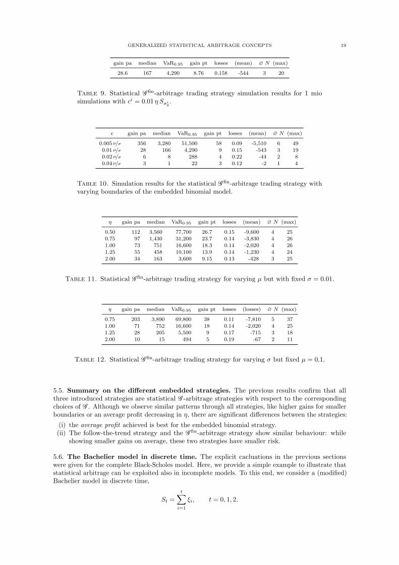
GENERALIZED STATISTICAL ARBITRAGE CONCEPTS 19
gain pa median VaR0.95 gain pt losses (mean) ∅ N (max)
28.6 167 4,290 8.76 0.158 -544 3 20
Table 9. Statistical G fin-arbitrage trading strategy simulation results for 1 miosimulations with ci = 0.01 η Sσi0 .
c gain pa median VaR0.95 gain pt losses (mean) ∅ N (max)
0.005 µ/σ 356 3,280 51,500 58 0.09 -5,510 6 49
0.01 µ/σ 28 166 4,290 9 0.15 -543 3 190.02 µ/σ 6 8 288 4 0.22 -44 2 8
0.04 µ/σ 3 1 22 3 0.12 -2 1 4
Table 10. Simulation results for the statistical G fin-arbitrage trading strategy withvarying boundaries of the embedded binomial model.
η gain pa median VaR0.95 gain pt losses (mean) ∅ N (max)
0.50 112 3,560 77,700 26.7 0.15 -9,600 4 25
0.75 97 1,430 31,200 23.7 0.14 -3,830 4 261.00 73 751 16,600 18.3 0.14 -2,020 4 26
1.25 55 458 10,100 13.9 0.14 -1,230 4 24
2.00 34 163 3,600 9.15 0.13 -428 3 25
Table 11. Statistical G fin-arbitrage trading strategy for varying µ but with fixed σ = 0.01.
η gain pa median VaR0.95 gain pt losses (losses) ∅ N (max)
0.75 203 3,890 69,800 38 0.11 -7,810 5 37
1.00 71 752 16,600 18 0.14 -2,020 4 251.25 28 205 5,500 9 0.17 -715 3 18
2.00 10 15 494 5 0.19 -67 2 11
Table 12. Statistical G fin-arbitrage trading strategy for varying σ but fixed µ = 0.1.
5.5. Summary on the different embedded strategies. The previous results confirm that allthree introduced strategies are statistical G -arbitrage strategies with respect to the correspondingchoices of G . Although we observe similar patterns through all strategies, like higher gains for smallerboundaries or an average profit decreasing in η, there are significant differences between the strategies:
(i) the average profit achieved is best for the embedded binomial strategy.(ii) The follow-the-trend strategy and the G fin-arbitrage strategy show similar behaviour: while
showing smaller gains on average, these two strategies have smaller risk.
5.6. The Bachelier model in discrete time. The explicit cacluations in the previous sectionswere given for the complete Black-Scholes model. Here, we provide a simple example to illustrate thatstatistical arbitrage can be exploited also in incomplete models. To this end, we consider a (modified)Bachelier model in discrete time,
St =
t∑i=1
ξi, t = 0, 1, 2.
20 CHRISTIAN REIN, LUDGER RUSCHENDORF, AND THORSTEN SCHMIDT
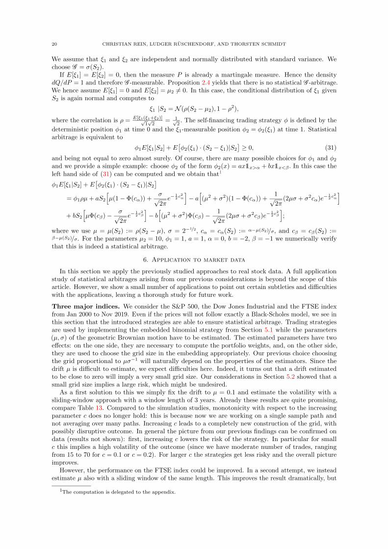
We assume that ξ1 and ξ2 are independent and normally distributed with standard variance. Wechoose G = σ(S2).
If E[ξ1] = E[ξ2] = 0, then the measure P is already a martingale measure. Hence the densitydQ/dP = 1 and therefore G -measurable. Proposition 2.4 yields that there is no statistical G -arbitrage.We hence assume E[ξ1] = 0 and E[ξ2] = µ2 6= 0. In this case, the conditional distribution of ξ1 givenS2 is again normal and computes to
ξ1 |S2 = N (ρ(S2 − µ2), 1− ρ2),
where the correlation is ρ = E[ξ1(ξ1+ξ2)]√1√
2= 1√
2. The self-financing trading strategy φ is defined by the
deterministic position φ1 at time 0 and the ξ1-measurable position φ2 = φ2(ξ1) at time 1. Statisticalarbitrage is equivalent to
φ1E[ξ1|S2] + E[φ2(ξ1) · (S2 − ξ1)|S2
]≥ 0, (31)
and being not equal to zero almost surely. Of course, there are many possible choices for φ1 and φ2
and we provide a simple example: choose φ2 of the form φ2(x) = ax1x>α + bx1x<β . In this case theleft hand side of (31) can be computed and we obtain that1
φ1E[ξ1|S2] + E[φ2(ξ1) · (S2 − ξ1)|S2
]= φ1ρµ+ aS2
[µ(1− Φ(cα)) +
σ√2πe−
12 c
2α
]− a[(µ2 + σ2)(1− Φ(cα)) +
1√2π
(2µσ + σ2cα)e−12 c
2α
]+ bS2
[µΦ(cβ)− σ√
2πe−
12 c
2β
]− b[(µ2 + σ2)Φ(cβ)− 1√
2π(2µσ + σ2cβ)e−
12 c
2β
];
where we use µ = µ(S2) := ρ(S2 − µ), σ = 2−1/2, cα = cα(S2) := α−µ(S2)/σ, and cβ = cβ(S2) :=β−µ(S2)/σ. For the parameters µ2 = 10, φ1 = 1, a = 1, α = 0, b = −2, β = −1 we numerically verifythat this is indeed a statistical arbitrage.
6. Application to market data
In this section we apply the previously studied approaches to real stock data. A full applicationstudy of statistical arbitrages arising from our previous considerations is beyond the scope of thisarticle. However, we show a small number of applications to point out certain subtleties and difficultieswith the applications, leaving a thorough study for future work.
Three major indices. We consider the S&P 500, the Dow Jones Industrial and the FTSE indexfrom Jan 2000 to Nov 2019. Even if the prices will not follow exactly a Black-Scholes model, we see inthis section that the introduced strategies are able to ensure statistical arbitrage. Trading strategiesare used by implementing the embedded binomial strategy from Section 5.1 while the parameters(µ, σ) of the geometric Brownian motion have to be estimated. The estimated parameters have twoeffects: on the one side, they are necessary to compute the portfolio weights, and, on the other side,they are used to choose the grid size in the embedding appropriately. Our previous choice choosingthe grid proportional to µσ−1 will naturally depend on the properties of the estimators. Since thedrift µ is difficult to estimate, we expect difficulties here. Indeed, it turns out that a drift estimatedto be close to zero will imply a very small grid size. Our considerations in Section 5.2 showed that asmall grid size implies a large risk, which might be undesired.
As a first solution to this we simply fix the drift to µ = 0.1 and estimate the volatility with asliding-window approach with a window length of 3 years. Already these results are quite promising,compare Table 13. Compared to the simulation studies, monotonicity with respect to the increasingparameter c does no longer hold: this is because now we are working on a single sample path andnot averaging over many paths. Increasing c leads to a completely new construction of the grid, withpossibly disruptive outcome. In general the picture from our previous findings can be confirmed ondata (results not shown): first, increasing c lowers the risk of the strategy. In particular for smallc this implies a high volatility of the outcome (since we have moderate number of trades, rangingfrom 15 to 70 for c = 0.1 or c = 0.2). For larger c the strategies get less risky and the overall pictureimproves.
However, the performance on the FTSE index could be improved. In a second attempt, we insteadestimate µ also with a sliding window of the same length. This improves the result dramatically, but
1The computation is delegated to the appendix.
GENERALIZED STATISTICAL ARBITRAGE CONCEPTS 21
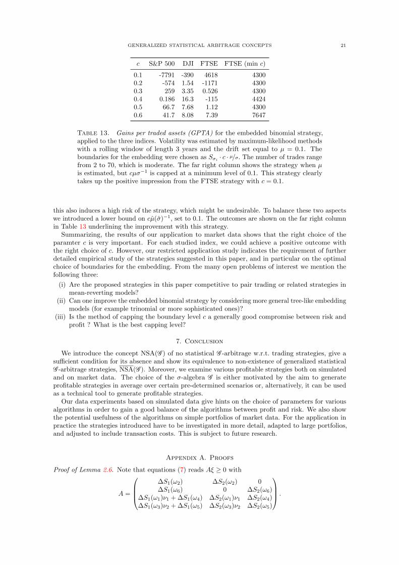
c S&P 500 DJI FTSE FTSE (min c)
0.1 -7791 -390 4618 43000.2 -574 1.54 -1171 43000.3 259 3.35 0.526 43000.4 0.186 16.3 -115 44240.5 66.7 7.68 1.12 43000.6 41.7 8.08 7.39 7647
Table 13. Gains per traded assets (GPTA) for the embedded binomial strategy,applied to the three indices. Volatility was estimated by maximum-likelihood methodswith a rolling window of length 3 years and the drift set equal to µ = 0.1. Theboundaries for the embedding were chosen as Sσi · c · µ/σ. The number of trades rangefrom 2 to 70, which is moderate. The far right column shows the strategy when µis estimated, but cµσ−1 is capped at a minimum level of 0.1. This strategy clearlytakes up the positive impression from the FTSE strategy with c = 0.1.
this also induces a high risk of the strategy, which might be undesirable. To balance these two aspectswe introduced a lower bound on cµ(σ)−1, set to 0.1. The outcomes are shown on the far right columnin Table 13 underlining the improvement with this strategy.
Summarizing, the results of our application to market data shows that the right choice of theparamter c is very important. For each studied index, we could achieve a positive outcome withthe right choice of c. However, our restricted application study indicates the requirement of furtherdetailed empirical study of the strategies suggested in this paper, and in particular on the optimalchoice of boundaries for the embedding. From the many open problems of interest we mention thefollowing three:
(i) Are the proposed strategies in this paper competitive to pair trading or related strategies inmean-reverting models?
(ii) Can one improve the embedded binomial strategy by considering more general tree-like embeddingmodels (for example trinomial or more sophisticated ones)?
(iii) Is the method of capping the boundary level c a generally good compromise between risk andprofit ? What is the best capping level?
7. Conclusion
We introduce the concept NSA(G ) of no statistical G -arbitrage w.r.t. trading strategies, give asufficient condition for its absence and show its equivalence to non-existence of generalized statisticalG -arbitrage strategies, NSA(G ). Moreover, we examine various profitable strategies both on simulatedand on market data. The choice of the σ-algebra G is either motivated by the aim to generateprofitable strategies in average over certain pre-determined scenarios or, alternatively, it can be usedas a technical tool to generate profitable strategies.
Our data experiments based on simulated data give hints on the choice of parameters for variousalgorithms in order to gain a good balance of the algorithms between profit and risk. We also showthe potential usefulness of the algorithms on simple portfolios of market data. For the application inpractice the strategies introduced have to be investigated in more detail, adapted to large portfolios,and adjusted to include transaction costs. This is subject to future research.
Appendix A. Proofs
Proof of Lemma 2.6. Note that equations (7) reads Aξ ≥ 0 with
A =
∆S1(ω2) ∆S2(ω2) 0∆S1(ω6) 0 ∆S2(ω6)
∆S1(ω1)ν1 + ∆S1(ω4) ∆S2(ω1)ν1 ∆S2(ω4)∆S1(ω3)ν2 + ∆S1(ω5) ∆S2(ω3)ν2 ∆S2(ω5)
.
22 CHRISTIAN REIN, LUDGER RUSCHENDORF, AND THORSTEN SCHMIDT
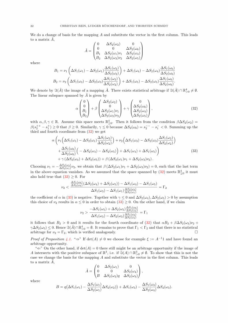
We do a change of basis for the mapping A and substitute the vector in the first column. This leadsto a matrix A,
A =
0 ∆S2(ω2) 00 0 ∆S2(ω6)B1 ∆S2(ω1)ν1 ∆S2(ω4)B2 ∆S2(ω3)ν2 ∆S2(ω5)
where
B1 = ν1
(∆S1(ω1)−∆S2(ω1)
∆S1(ω2)
∆S2(ω2)
)+ ∆S1(ω4)−∆S2(ω4)
∆S1(ω6)
∆S2(ω6)
B2 = ν2
(∆S1(ω3)−∆S2(ω3)
∆S1(ω2)
∆S2(ω2)
)+ ∆S1(ω5)−∆S2(ω5)
∆S1(ω6)
∆S2(ω6).
We denote by =(A) the image of a mapping A. There exists statistical arbitrage if =(A) ∩ R4>0 6= ∅.
The linear subspace spanned by A is given by
α
00B1
B2
+ β
∆S2(ω2)
0∆S2(ω1)ν1
∆S2(ω3)ν2
+ γ
0
∆S2(ω6)∆S2(ω4)∆S2(ω5)
, (32)
with α, β, γ ∈ R. Assume this space meets R4≥0. Then it follows from the condition β∆S2(ω2) =
β(s++2 − s+
1 ) ≥ 0 that β ≥ 0. Similarily, γ ≤ 0 because ∆S2(ω6) = s−−2 − s−1 < 0. Summing up thethird and fourth coordinate from (32) we get
α
(ν1
(∆S1(ω1)−∆S2(ω1)
∆S1(ω2)
∆S2(ω2)
)+ ν2
(∆S1(ω3)−∆S2(ω3)
∆S1(ω2)
∆S2(ω2)
)+
∆S1(ω6)
∆S2(ω6)
(−∆S2(ω4)−∆S2(ω5)
)+ ∆S1(ω4) + ∆S1(ω5)
)(33)
+ γ (∆S2(ω4) + ∆S2(ω5)) + β (∆S2(ω1)ν1 + ∆S2(ω3)ν2) .
Choosing ν1 = −∆S2(ω3)∆S2(ω1)ν2, we obtain that β (∆S2(ω1)ν1 + ∆S2(ω3)ν2) = 0, such that the last term
in the above equation vanishes. As we assumed that the space spanned by (32) meets R4≥0 it must
also hold true that (33) ≥ 0. For
ν2 <
∆S1(ω6)∆S2(ω6) (∆S2(ω4) + ∆S2(ω5))−∆S1(ω4)−∆S1(ω5)
∆S1(ω3)−∆S1(ω1)∆S2(ω3)∆S2(ω1)
= Γ2
the coefficient of α in (33) is negative. Together with γ ≤ 0 and ∆S2(ω4),∆S2(ω5) > 0 by assumptionthis choice of ν2 results in α ≤ 0 in order to obtain (33) ≥ 0. On the other hand, if we claim
ν2 >−∆S1(ω5) + ∆S2(ω5)∆S1(ω6)
∆S2(ω6)
∆S1(ω3)−∆S2(ω3)∆S1(ω2)∆S2(ω2)
= Γ1
it follows that B2 > 0 and it results for the fourth coordinate of (32) that αB2 + β∆S2(ω3)ν2 +
γ∆S2(ω5) ≤ 0. Hence =(A)∩R4>0 = ∅. It remains to prove that Γ1 < Γ2 and that there is no statistical
arbitrage for ν2 = Γ2, which is verified analogously.
Proof of Proposition 4.1. “⇒” If det(A) 6= 0 we choose for example ξ := A−11 and have found anarbitrage opportunity.
“⇐” On the other hand, if det(A) = 0 there still might be an arbitrage opportunity if the image ofA intersects with the positive subspace of R3, i.e. if =(A) ∩ R3
>0 6= ∅. To show that this is not thecase we change the basis for the mapping A and substitute the vector in the first column. This leadsto a matrix A,
A =
0 ∆S2(ω1) 00 0 ∆S2(ω4)B ∆S2(ω2)q ∆S2(ω3)
,
where
B = q(∆S1(ω1)− ∆S1(ω1)
∆S2(ω1)∆S2(ω2)
)+ ∆S1(ω3)− ∆S1(ω3)
∆S2(ω4)∆S2(ω3).
GENERALIZED STATISTICAL ARBITRAGE CONCEPTS 23
Hence, 0 = det(A) = B∆S2(ω1)∆S2(ω4) leading to B = 0. In this case the linear subspace spanned
by A is given by
α
∆S2(ω1)0
q∆S2(ω2)
+ β
0∆S2(ω4)∆S2(ω3)
, (34)
with α, β ∈ R. Because ∆S2(ω1) > 0 we need α ≥ 0 to have arbitrage opportunities. Similar we needto have β ≤ 0 because of ∆S2(ω4) < 0 by assumption. But, as ∆S2(ω2) < 0 and ∆S2(ω3) > 0, weobtain for the third coordinate that αq∆S2(ω2) + β∆S2(ω3) ≤ 0 and hence =(A) ∩ R3
>0 = ∅, whichprooves the first part. For the second part, we simply compute det(A) from Equation (13).
Proof of Proposition 5.1. Following Definition 2.1 the strategy ψ is a statistical G -arbitrage strategyif the following holds
ψ1∆S1(ω1) + ψ+2 ∆S2(ω1) + ψ++
3 ∆S3(ω1) ≥ 0
ψ1∆S1(ω4) + ψ−2 ∆S2(ω4) ≥ 0
ψ1∆S1(ω2)P (ω2) + ψ+2 ∆S2(ω2)P (ω2) + ψ1∆S1(ω3)P (ω3) + ψ−2 ∆S2(ω3)P (ω3) ≥ 0,
ψ1∆S1(ω5) + ψ+2 ∆S2(ω5) + ψ++
3 ∆S3(ω5) ≥ 0
(35)
and, in addition, at least one of the inequalities is strict. We extend the setting from Lemma 4.2.First, we let
A =
∆S1(ω1) ∆S2(ω1) 0 ∆S3(ω1)∆S1(ω4) 0 ∆S2(ω4) 0
q∆S1(ω2) + ∆S1(ω3) q∆S2(ω2) ∆S2(ω3) 0∆S1(ω5) ∆S2(ω5) 0 ∆S3(ω5)
.
Then Equations (35) are equivalent to Aψ ≥ 0. Note that Si(ω1) = Si(ω5) for i = 1, 2 such that
Aψ = x with x = (x1, . . . , x4)> reveals
ψ++3 =
x1 − x4
∆S3(ω1)−∆S3(ω5).
As for Lemma 4.2, we will consider the case where A is invertible. Note that the three times threesubmatrix (upper left) of A equals the matrix A from Equation (13). Then, denoting x = (x1, x2, x3)>,ψ1
ψ+2
ψ−2
= A−1x−A−1
∆S3(ω1)ψ++3
00
= A−1x−∆S3(ω1)ψ++3 γ
with vector γ from Equation (26). Up to now we where free to choose any x ∈ R4>0. If we choose
x = 13, then φ = A−113 is the strategy computed in Lemma 4.2 and the result follows.
Appendix B. Computation of a specific example of Equation (31)
Consider a random variable ξ ∼ N (µ, σ2), such that ξ = µ+ ση with standard normal η. Then itis easy to verify that
E[ξ1ξ>α] = E[µ1η>cα] + σE[η1η>cα] = µ(1− Φ(cα)) +σ√2πe−
12 c
2α ,
E[ξ21ξ>α] = (µ2 + σ2)(1− Φ(cα)) +1√2π
(2µσ + σ2cα)e−12 c
2α ,
E[ξ1ξ<β] = µΦ(cβ)− σ√2πe−
12 c
2β ,
E[ξ21ξ<β] = (µ2 + σ2)Φ(cβ)− 1√2π
(2µσ + σ2cβ)e−12 c
2β .
Now, we obtain E[φ2(ξ1)(S2 − ξ1)|S2 = s] = E[φ2(ξ)(s − ξ)], where µ = µ(s) = ρ(s − µ2) andξ ∼ N (µ, σ2). Using the specific form of φ2 and the above computations gives the result.
24 CHRISTIAN REIN, LUDGER RUSCHENDORF, AND THORSTEN SCHMIDT
References
Ananova, A., Cont, R. and Xu, R. (2020), ‘Excursion risk’, arXiv preprint arXiv:2011.02870 .Avellaneda, M. and Lee, J.-H. (2010), ‘Statistical arbitrage in the US equities market’, Quantitative
Finance 10(7), 761–782.Bernardo, A. E. and Ledoit, O. (2000), ‘Gain, loss, and asset pricing’, Journal of political economy
108(1), 144–172.Bondarenko, O. (2003), ‘Statistical arbitrage and securities prices’, The Review of Financial Studies
16(3), 875–919.Borodin, A. N. and Salminen, P. (2012), Handbook of Brownian motion-facts and formulae, Birkhauser.Burgert, C. and Ruschendorf, L. (2006), ‘On the optimal risk allocation problem’, Statistics & decisions
24(1/2006), 153–171.Cerny, A. and Hodges, S. (2002), The theory of good-deal pricing in financial markets, in ‘Mathematical
Finance—Bachelier Congress 2000’, Springer, pp. 175–202.Cochrane, J. H. and Saa-Requejo, J. (2000), ‘Beyond arbitrage: Good-deal asset price bounds in
incomplete markets’, Journal of political economy 108(1), 79–119.Delbaen, F. and Schachermayer, W. (1995), ‘The no-arbitrage property under a change of numeraire’,
Stochastics and Stochastic Reports 53(3-4), 213–226.Delbaen, F. and Schachermayer, W. (2006), The mathematics of arbitrage, Springer Science & Business
Media.Elliott, R. J., Van Der Hoek, J. and Malcolm, W. P. (2005), ‘Pairs trading’, Quantitative Finance
5(3), 271–276.Gatev, E., Goetzmann, W. N. and Rouwenhorst, K. G. (2006), ‘Pairs trading: Performance of a
relative-value arbitrage rule’, The Review of Financial Studies 19(3), 797–827.Goncu, A. (2015), ‘Statistical arbitrage in the Black–Scholes framework’, Quantitative Finance
15(9), 1489–1499.Hansen, L. P. and Jagannathan, R. (1991), ‘Implications of security market data for models of dynamic
economies’, Journal of political economy 99(2), 225–262.Hogan, S., Jarrow, R., Teo, M. and Warachka, M. (2004), ‘Testing market efficiency using statistical
arbitrage with applications to momentum and value strategies’, Journal of Financial economics73(3), 525–565.
Kassberger, S. and Liebmann, T. (2017), ‘Additive portfolio improvement and utility-efficient payoffs’,Mathematics and Financial Economics 11(2), 241–262.
Krauss, C. (2017), ‘Statistical arbitrage pairs trading strategies: Review and outlook’, Journal ofEconomic Surveys 31(2), 513–545.
Lazzarino, M., Berrill, J. and Sevic, A. (2018), ‘What is statistical arbitrage?’, Theoretical EconomicsLetters 8(05), 888.
University of Freiburg, Department of Mathematical Stochastics, Ernst-Zermelo-Str. 1, 79104 Freiburg,Germany
Email address: [email protected]
Email address: [email protected]
Email address: [email protected]