Generalized Nonlinear Models in R

Generalized Nonlinear Models in R

Heather Turner1,2, David Firth2 and Ioannis Kosmidis3

1 Independent consultant2 University of Warwick, UK

3 UCL, UK

Turner, Firth & Kosmidis GNM in R ERCIM 2013 1 / 30

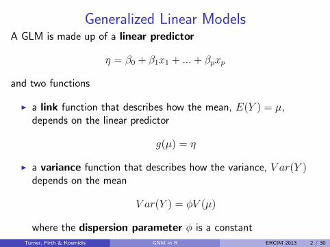
Generalized Linear ModelsA GLM is made up of a linear predictor

η = β0 + β1x1 + ...+ βpxp

and two functions

I a link function that describes how the mean, E(Y ) = µ,depends on the linear predictor

g(µ) = η

I a variance function that describes how the variance, V ar(Y )depends on the mean

V ar(Y ) = φV (µ)

where the dispersion parameter φ is a constantTurner, Firth & Kosmidis GNM in R ERCIM 2013 2 / 30

Generalized Nonlinear Models

A generalized nonlinear model (GNM) is the same as a GLMexcept that we have

g(µ) = η(x; β)

where η(x; β) is nonlinear in the parameters β.

Equivalently an extension of nonlinear least squares model, where thevariance of Y is allowed to depend on the mean.

Using a nonlinear predictor can produce a more parsimonious andinterpretable model.


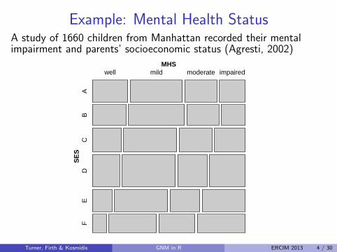
Example: Mental Health StatusA study of 1660 children from Manhattan recorded their mentalimpairment and parents’ socioeconomic status (Agresti, 2002)

MHS

SE

SF

ED

CB

A

well mild moderate impaired


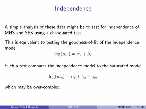
Independence

A simple analysis of these data might be to test for independence ofMHS and SES using a chi-squared test.

This is equivalent to testing the goodness-of-fit of the independencemodel

log(µrc) = αr + βc

Such a test compares the independence model to the saturated model

log(µrc) = αr + βc + γrc

which may be over-complex.


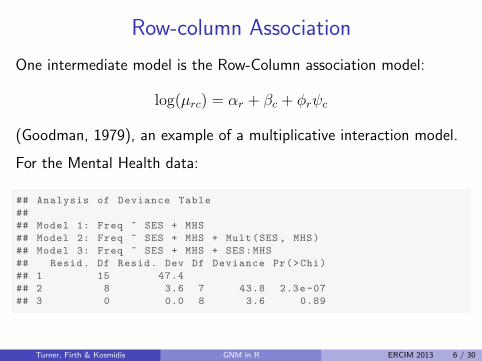
Row-column Association

One intermediate model is the Row-Column association model:

log(µrc) = αr + βc + φrψc

(Goodman, 1979), an example of a multiplicative interaction model.

For the Mental Health data:

## Analysis of Deviance Table

##

## Model 1: Freq ~ SES + MHS

## Model 2: Freq ~ SES + MHS + Mult(SES , MHS)

## Model 3: Freq ~ SES + MHS + SES:MHS

## Resid. Df Resid. Dev Df Deviance Pr(>Chi)

## 1 15 47.4

## 2 8 3.6 7 43.8 2.3e-07

## 3 0 0.0 8 3.6 0.89


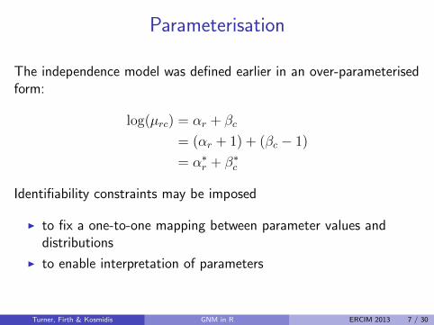
Parameterisation

The independence model was defined earlier in an over-parameterisedform:

log(µrc) = αr + βc

= (αr + 1) + (βc − 1)

= α∗r + β∗

c

Identifiability constraints may be imposed

I to fix a one-to-one mapping between parameter values anddistributions

I to enable interpretation of parameters


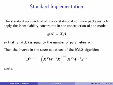
Standard Implementation

The standard approach of all major statistical software packages is toapply the identifiability constraints in the construction of the model

g(µ) =Xβ

so that rank(X) is equal to the number of parameters p.

Then the inverse in the score equations of the IWLS algorithm

β(r+1) =(XTW (r)X

)−1

XTW (r)z(r)

exists.


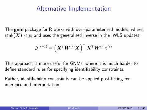
Alternative Implementation

The gnm package for R works with over-parameterised models, whererank(X) < p, and uses the generalised inverse in the IWLS updates:

β(r+1) =(XTW (r)X

)−XTW (r)z(r)

This approach is more useful for GNMs, where it is much harder todefine standard rules for specifying identifiability constraints.

Rather, identifiability constraints can be applied post-fitting forinference and interpretation.


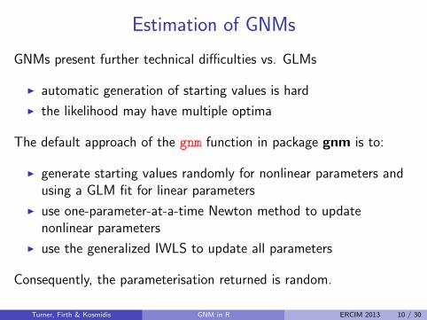
Estimation of GNMs

GNMs present further technical difficulties vs. GLMs

I automatic generation of starting values is hard

I the likelihood may have multiple optima

The default approach of the gnm function in package gnm is to:

I generate starting values randomly for nonlinear parameters andusing a GLM fit for linear parameters

I use one-parameter-at-a-time Newton method to updatenonlinear parameters

I use the generalized IWLS to update all parameters

Consequently, the parameterisation returned is random.


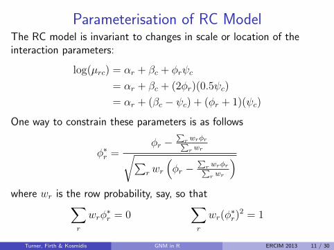
Parameterisation of RC ModelThe RC model is invariant to changes in scale or location of theinteraction parameters:

log(µrc) = αr + βc + φrψc

= αr + βc + (2φr)(0.5ψc)

= αr + (βc − ψc) + (φr + 1)(ψc)

One way to constrain these parameters is as follows

φ∗r =

φr −∑

r wrφr∑r wr√∑

r wr

(φr −

∑r wrφr∑r wr

)where wr is the row probability, say, so that∑

r

wrφ∗r = 0

∑r

wr(φ∗r)

2 = 1


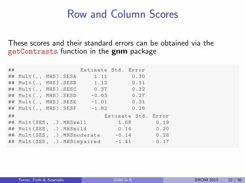
Row and Column Scores

These scores and their standard errors can be obtained via thegetContrasts function in the gnm package

## Estimate Std. Error

## Mult(., MHS).SESA 1.11 0.30

## Mult(., MHS).SESB 1.12 0.31

## Mult(., MHS).SESC 0.37 0.32

## Mult(., MHS).SESD -0.03 0.27

## Mult(., MHS).SESE -1.01 0.31

## Mult(., MHS).SESF -1.82 0.28

## Estimate Std. Error

## Mult(SES , .).MHSwell 1.68 0.19

## Mult(SES , .).MHSmild 0.14 0.20

## Mult(SES , .).MHSmoderate -0.14 0.28

## Mult(SES , .).MHSimpaired -1.41 0.17


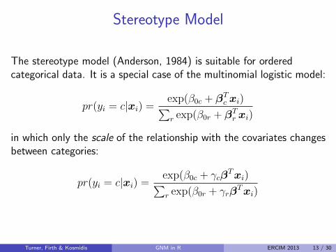
Stereotype Model

The stereotype model (Anderson, 1984) is suitable for orderedcategorical data. It is a special case of the multinomial logistic model:

pr(yi = c|xi) =exp(β0c + β

Tc xi)∑

r exp(β0r + βTr xi)

in which only the scale of the relationship with the covariates changesbetween categories:

pr(yi = c|xi) =exp(β0c + γcβ

Txi)∑r exp(β0r + γrβ

Txi)


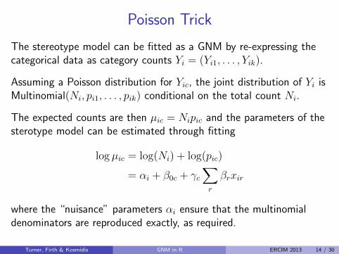
Poisson Trick

The stereotype model can be fitted as a GNM by re-expressing thecategorical data as category counts Yi = (Yi1, . . . , Yik).

Assuming a Poisson distribution for Yic, the joint distribution of Yi isMultinomial(Ni, pi1, . . . , pik) conditional on the total count Ni.

The expected counts are then µic = Nipic and the parameters of thesterotype model can be estimated through fitting

log µic = log(Ni) + log(pic)

= αi + β0c + γc∑r

βrxir

where the “nuisance” parameters αi ensure that the multinomialdenominators are reproduced exactly, as required.


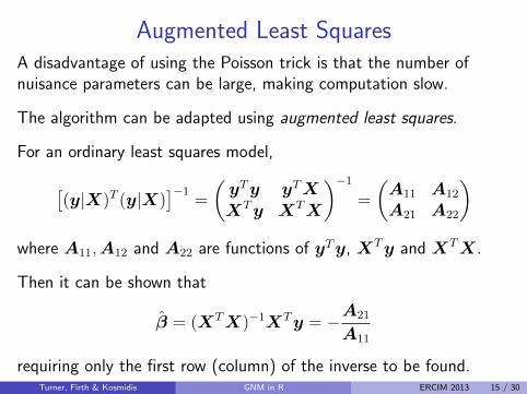
Augmented Least SquaresA disadvantage of using the Poisson trick is that the number ofnuisance parameters can be large, making computation slow.

The algorithm can be adapted using augmented least squares.

For an ordinary least squares model,

[(y|X)T (y|X)

]−1=

(yTy yTXXTy XTX

)−1

=

(A11 A12

A21 A22

)where A11,A12 and A22 are functions of yTy, XTy and XTX.

Then it can be shown that

β̂ = (XTX)−1XTy = −A21

A11

requiring only the first row (column) of the inverse to be found.Turner, Firth & Kosmidis GNM in R ERCIM 2013 15 / 30

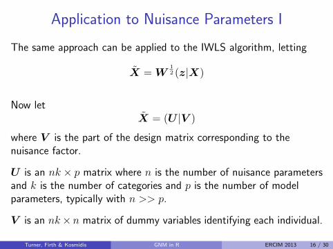
Application to Nuisance Parameters I

The same approach can be applied to the IWLS algorithm, letting

X̃ =W12 (z|X)

Now letX̃ = (U |V )

where V is the part of the design matrix corresponding to thenuisance factor.

U is an nk × p matrix where n is the number of nuisance parametersand k is the number of categories and p is the number of modelparameters, typically with n >> p.

V is an nk×n matrix of dummy variables identifying each individual.


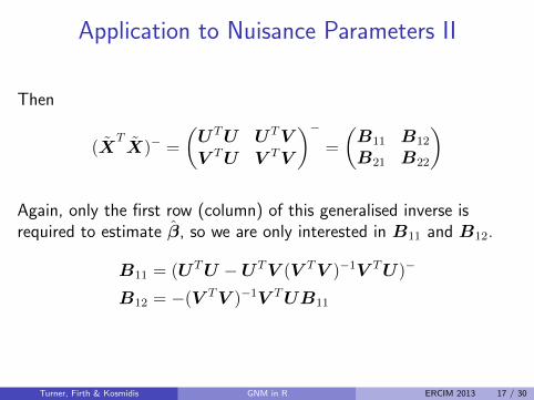
Application to Nuisance Parameters II

Then

(X̃TX̃)− =

(UTU UTVV TU V TV

)−

=

(B11 B12

B21 B22

)

Again, only the first row (column) of this generalised inverse isrequired to estimate β̂, so we are only interested in B11 and B12.

B11 = (UTU −UTV (V TV )−1V TU)−

B12 = −(V TV )−1V TUB11


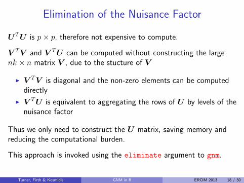
Elimination of the Nuisance Factor

UTU is p× p, therefore not expensive to compute.

V TV and V TU can be computed without constructing the largenk × n matrix V , due to the stucture of V

I V TV is diagonal and the non-zero elements can be computeddirectly

I V TU is equivalent to aggregating the rows of U by levels of thenuisance factor

Thus we only need to construct the U matrix, saving memory andreducing the computational burden.

This approach is invoked using the eliminate argument to gnm.


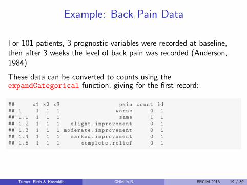
Example: Back Pain Data

For 101 patients, 3 prognostic variables were recorded at baseline,then after 3 weeks the level of back pain was recorded (Anderson,1984)

These data can be converted to counts using theexpandCategorical function, giving for the first record:

## x1 x2 x3 pain count id

## 1 1 1 1 worse 0 1

## 1.1 1 1 1 same 1 1

## 1.2 1 1 1 slight.improvement 0 1

## 1.3 1 1 1 moderate.improvement 0 1

## 1.4 1 1 1 marked.improvement 0 1

## 1.5 1 1 1 complete.relief 0 1


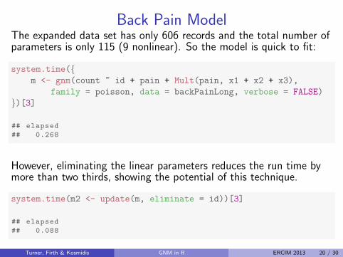
Back Pain ModelThe expanded data set has only 606 records and the total number ofparameters is only 115 (9 nonlinear). So the model is quick to fit:

system.time({m <- gnm(count ~ id + pain + Mult(pain, x1 + x2 + x3),

family = poisson, data = backPainLong, verbose = FALSE)

})[3]

## elapsed

## 0.268

However, eliminating the linear parameters reduces the run time bymore than two thirds, showing the potential of this technique.

system.time(m2 <- update(m, eliminate = id))[3]

## elapsed

## 0.088


Rasch Models

Rasch models are used in Item Response Theory to model the binaryresponses of subjects over a set of items.

The simplest one parameter logistic (1PL) model has the form

logπis

1− πis= αi + γs

The one-dimensional Rasch model extends the 1PL as follows:

logπis

1− πis= αi + βiγs

where βi measures the discrimination of item i: the larger βi thesteeper the item-response function that maps γs to πis.


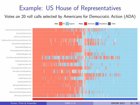
Example: US House of RepresentativesVotes on 20 roll calls selected by Americans for Democratic Action (ADA)

BankruptcyOverhaul.Yes

ErgonomicsRuleDisapproval.No

IncomeTaxReduction.No

MarriageTaxReduction.Yes

EstateTaxRelief.Yes

FetalProtection.No

SchoolVouchers.No

TaxCutReconciliationBill.No

CampaignFinanceReform.No

FlagDesecration.No

FaithBasedInitiative.Yes

ChinaNormalizedTradeRelations.Yes

ANWRDrillingBan.Yes

PatientsRightsHMOLiability.No

PatientsBillOfRights.No

DomesticPartnerBenefits.No

USMilitaryPersonnelOverseasAbortions.Yes

AntiTerrorismAuthority.No

EconomicStimulus.No

TradePromotionAuthorityFastTrack.No

Vote For Against Party Democrat Republican Other


Complete Separation

For representatives that always vote “For” or “Against” the ASAposition, maximum likelihood will produce infinite γs estimates, sothat the fitted probabilities are 0 or 1.

Two possible remedies:

1. Add δ to yis and 2δ to the totals nisI hard to quantify effect of adjustmentI different δ give different results

2. Bias reduction (Firth, 1993; Kosmidis and Firth, 2009)I requires identifiable parameterization


Bias Reduction in the 1D Rasch Model

ML estimates are obtained by solving the score equations, which forthe one dimensional Rasch model with θ = (αT , βT , γT )T are

Ut =I∑i=1

S∑s=1

(yis − nisπis)zist = 0

where zist = ∂ηis/∂θt.

The bias reduction method of Kosmidis and Firth (2009) works byadjusting the scores, in this case giving

U∗t =

I∑i=1

S∑s=1

{yis +

1

2his + cisvis − (nis + his)πis

}zist = 0

where vis, his and cis are depend on the model parameters.


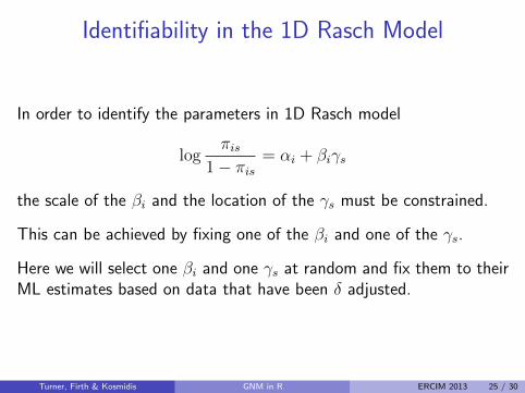
Identifiability in the 1D Rasch Model

In order to identify the parameters in 1D Rasch model

logπis

1− πis= αi + βiγs

the scale of the βi and the location of the γs must be constrained.

This can be achieved by fixing one of the βi and one of the γs.

Here we will select one βi and one γs at random and fix them to theirML estimates based on data that have been δ adjusted.


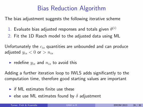
Bias Reduction Algorithm

The bias adjustment suggests the following iterative scheme

1. Evaluate bias adjusted responses and totals given θ(i)

2. Fit the 1D Rasch model to the adjusted data using ML

Unfortunately the cis quantities are unbounded and can produceadjusted yis < 0 or > nis

I redefine yis and nis to avoid this

Adding a further iteration loop to IWLS adds significantly to thecomputation time, therefore good starting values are important

I if ML estimates finite use these

I else use ML estimates found by δ adjustment


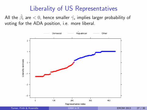
Liberality of US RepresentativesAll the β̂i are < 0, hence smaller γ̂s implies larger probability ofvoting for the ADA position, i.e. more liberal.


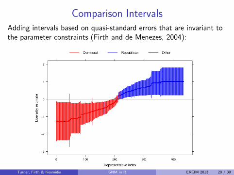
Comparison IntervalsAdding intervals based on quasi-standard errors that are invariant tothe parameter constraints (Firth and de Menezes, 2004):


Summary

I Working with over-parameterized models enables a generalframework to be implemented for GNMs

I Some of the computational methods from GLMs can be applieddirectly to GNMs. . .

I . . . whilst others require much more work!

I Further examples can be found in the help files and manualaccompanying the gnm package which is available on CRAN.


References

Agresti, A. (2002). Categorical Data Analysis (2nd ed.). New York: Wiley.

Anderson, J. A. (1984). Regression and Ordered Categorical Variables. J.R. Statist. Soc. B 46(1), 1–30.

Firth, D. (1993). Bias reduction of maximum likelihood estimates.Biometrika 80(1), 27–38.

Firth, D. and R. X. de Menezes (2004). Quasi-variances. Biometrika 91,65–80.

Goodman, L. A. (1979). Simple models for the analysis of association incross-classifications having ordered categories. J. Amer. Statist.Assoc. 74, 537–552.

Kosmidis, I. and D. Firth (2009). Bias reduction in exponential familynonlinear models. Biometrika 96(4), 793–804.


Generalized Nonlinear Models in R

Data & Analytics

Transcript of Generalized Nonlinear Models in R