General state space Markov chains and MCMC algorithms · General state space Markov chains and ......

arX

iv:m

ath/

0404

033v

4 [

mat

h.PR

] 1

1 A

pr 2

007

Probability Surveys

Vol. 1 (2004) 20–71ISSN: 1549-5787DOI: 10.1214/154957804100000024

General state space Markov chains and

MCMC algorithms∗

Gareth O. Roberts

Department of Mathematics and Statistics, Fylde College, Lancaster University, Lancaster,LA1 4YF, England

e-mail: [email protected]

Jeffrey S. Rosenthal†

Department of Statistics, University of Toronto, Toronto, Ontario, Canada M5S 3G3e-mail: [email protected]

Abstract: This paper surveys various results about Markov chains on gen-eral (non-countable) state spaces. It begins with an introduction to Markovchain Monte Carlo (MCMC) algorithms, which provide the motivation andcontext for the theory which follows. Then, sufficient conditions for geomet-ric and uniform ergodicity are presented, along with quantitative boundson the rate of convergence to stationarity. Many of these results are provedusing direct coupling constructions based on minorisation and drift con-ditions. Necessary and sufficient conditions for Central Limit Theorems(CLTs) are also presented, in some cases proved via the Poisson Equa-tion or direct regeneration constructions. Finally, optimal scaling and weakconvergence results for Metropolis-Hastings algorithms are discussed. Noneof the results presented is new, though many of the proofs are. We alsodescribe some Open Problems.

Received March 2004.

1. Introduction

Markov chain Monte Carlo (MCMC) algorithms – such as the Metropolis-Hastings algorithm ([53], [37]) and the Gibbs sampler (e.g. Geman and Ge-man [32]; Gelfand and Smith [30]) – have become extremely popular in statis-tics, as a way of approximately sampling from complicated probability distribu-tions in high dimensions (see for example the reviews [93], [89], [33], [71]). Mostdramatically, the existence of MCMC algorithms has transformed Bayesian in-ference, by allowing practitioners to sample from posterior distributions of com-plicated statistical models.

In addition to their importance to applications in statistics and other sub-jects, these algorithms also raise numerous questions related to probability the-ory and the mathematics of Markov chains. In particular, MCMC algorithmsinvolve Markov chains {Xn} having a (complicated) stationary distribution π(·),for which it is important to understand as precisely as possible the nature andspeed of the convergence of the law of Xn to π(·) as n increases.

∗This is an original survey paper.†Web: http://probability.ca/jeff/ . Supported in part by NSERC of Canada.

20

http://arXiv.org/abs/math/0404033v4

http://stat-www.berkeley.edu/users/prsurvey

http://dx.doi.org/10.1214/154957804100000024

mailto:[email protected]

mailto:[email protected]

http://probability.ca/jeff/

G.O. Roberts, J.S. Rosenthal/Markov chains and MCMC algorithms 21

This paper attempts to explain and summarise MCMC algorithms and theprobability theory questions that they generate. After introducing the algo-rithms (Section 2), we discuss various important theoretical questions relatedto them. In Section 3 we present various convergence rate results commonlyused in MCMC. Most of these are proved in Section 4, using direct couplingarguments and thereby avoiding many of the analytic technicalities of previousproofs. We consider MCMC central limit theorems in Section 5, and optimalscaling and weak convergence results in Section 6. Numerous references to theMCMC literature are given throughout. We also describe some Open Problems.

1.1. The problem

The problem addressed by MCMC algorithms is the following. We’re given adensity function πu, on some state space X , which is possibly unnormalised butat least satisfies 0 <

∫

X πu < ∞. (Typically X is an open subset of Rd, and thedensities are taken with respect to Lebesgue measure, though other settings –including discrete state spaces – are also possible.) This density gives rise to aprobability measure π(·) on X , by

π(A) =

∫

Aπu(x)dx

∫

X πu(x)dx. (1)

We want to (say) estimate expectations of functions f : X → R with respectto π(·), i.e. we want to estimate

π(f) = Eπ[f(X)] =

∫

X f(x)πu(x)dx∫

X πu(x)dx. (2)

If X is high-dimensional, and πu is a complicated function, then direct integra-tion (either analytic or numerical) of the integrals in (2) is infeasible.

The classical Monte Carlo solution to this problem is to simulate i.i.d. ran-dom variables Z1, Z2, . . . , ZN ∼ π(·), and then estimate π(f) by

π(f) = (1/N)

N∑

i=1

f(Zi). (3)

This gives an unbiased estimate, having standard deviation of order O(1/√

N).Furthermore, if π(f2) < ∞, then by the classical Central Limit Theorem, theerror π(f) − π(f) will have a limiting normal distribution, which is also useful.The problem, however, is that if πu is complicated, then it is very difficult todirectly simulate i.i.d. random variables from π(·).

The Markov chain Monte Carlo (MCMC) solution is to instead construct aMarkov chain on X which is easily run on a computer, and which has π(·) asa stationary distribution. That is, we want to define easily-simulated Markovchain transition probabilities P (x, dy) for x, y ∈ X , such that

∫

x∈Xπ(dx)P (x, dy) = π(dy). (4)


Then hopefully (see Subsection 3.2), if we run the Markov chain for a longtime (started from anywhere), then for large n the distribution of Xn will beapproximately stationary: L(Xn) ≈ π(·). We can then (say) set Z1 = Xn, andthen restart and rerun the Markov chain to obtain Z2, Z3, etc., and then doestimates as in (3).

It may seem at first to be even more difficult to find such a Markov chain,then to estimate π(f) directly. However, we shall see in the next section thatconstructing (and running) such Markov chains is often surprisingly straightfor-ward.

Remark. In the practical use of MCMC, rather than start a fresh Markovchain for each new sample, often an entire tail of the Markov chain run {Xn} is

used to create an estimate such as (N −B)−1∑N

i=B+1 f(Xi), where the burn-invalue B is hopefully chosen large enough that L(XB) ≈ π(·). In that case thedifferent f(Xi) are not independent, but the estimate can be computed moreefficiently. Since many of the mathematical issues which arise are similar ineither implementation, we largely ignore this modification herein.

Remark. MCMC is, of course, not the only way to sample or estimate fromcomplicated probability distributions. Other possible sampling algorithms in-clude “rejection sampling” and “importance sampling”, not reviewed here; butthese alternative algorithms only work well in certain particular cases and arenot as widely applicable as MCMC algorithms.

1.2. Motivation: Bayesian Statistics Computations

While MCMC algorithms are used in many fields (statistical physics, computerscience), their most widespread application is in Bayesian statistical inference.

Let L(y|θ) be the likelihood function (i.e., density of data y given unknownparameters θ) of a statistical model, for θ ∈ X . (Usually X ⊆ Rd.) Let the“prior” density of θ be p(θ). Then the “posterior” distribution of θ given y isthe density which is proportional to

πu(θ) ≡ L(y | θ) p(θ).

(Of course, the normalisation constant is simply the density for the data y,though that constant may be impossible to compute.) The “posterior mean” ofany functional f is then given by:

π(f) =

∫

X f(x)πu(x)dx∫

X πu(x)dx.

For this reason, Bayesians are anxious (even desperate!) to estimate suchπ(f). Good estimates allow Bayesian inference can be used to estimate a widevariety of parameters, probabilities, means, etc. MCMC has proven to be ex-tremely helpful for such Bayesian estimates, and MCMC is now extremely widelyused in the Bayesian statistical community.


2. Constructing MCMC Algorithms

We see from the above that an MCMC algorithm requires, given a probabilitydistribution π(·) on a state space X , a Markov chain on X which is easilyrun on a computer, and which has π(·) as its stationary distribution as in (4).This section explains how such Markov chains are constructed. It thus providesmotivation and context for the theory which follows; however, for the readerinterested purely in the mathematical results, this section can be omitted withlittle loss of continuity.

A key notion is reversibility, as follows.

Definition. A Markov chain on a state space X is reversible with respect to aprobability distribution π(·) on X , if

π(dx)P (x, dy) = π(dy)P (y, dx), x, y ∈ X .

A very important property of reversibility is the following.

Proposition 1. If Markov chain is reversible with respect to π(·), then π(·) isstationary for the chain.

Proof. We compute that∫

x∈Xπ(dx)P (x, dy) =

∫

x∈Xπ(dy)P (y, dx) = π(dy)

∫

x∈XP (y, dx) = π(dy).

We see from this lemma that, when constructing an MCMC algorithm, itsuffices to create a Markov chain which is easily run, and which is reversiblewith respect to π(·). The simplest way to do so is to use the Metropolis-Hastingsalgorithm, as we now discuss.

2.1. The Metropolis-Hastings Algorithm

Suppose again that π(·) has a (possibly unnormalised) density πu, as in (1).Let Q(x, ·) be essentially any other Markov chain, whose transitions also havea (possibly unnormalised) density, i.e. Q(x, dy) ∝ q(x, y) dy.

The Metropolis-Hastings algorithm proceeds as follows. First choose some X0.Then, given Xn, generate a proposal Yn+1 from Q(Xn, ·). Also flip an indepen-dent coin, whose probability of heads equals α(Xn, Yn+1), where

α(x, y) = min

[

1,πu(y) q(y, x)

πu(x) q(x, y)

]

.

(To avoid ambiguity, we set α(x, y) = 1 whenever π(x) q(x, y) = 0.) Then, ifthe coin is heads, “accept” the proposal by setting Xn+1 = Yn+1; if the coin istails then “reject” the proposal by setting Xn+1 = Xn. Replace n by n + 1 andrepeat.

The reason for the unusual formula for α(x, y) is the following:


Proposition 2. The Metropolis-Hastings algorithm (as described above) pro-duces a Markov chain {Xn} which is reversible with respect to π(·).Proof. We need to show

π(dx)P (x, dy) = π(dy)P (y, dx).

It suffices to assume x 6= y (since if x = y then the equation is trivial). But forx 6= y, setting c =

∫

X πu(x) dx,

π(dx)P (x, dy) = [c−1πu(x) dx] [q(x, y)α(x, y) dy]

= c−1πu(x) q(x, y) min

[

1,πu(y)q(y, x)

πu(x)q(x, y)

]

dx dy

= c−1 min[πu(x) q(x, y), πu(y)q(y, x)] dx dy,

which is symmetric in x and y.

To run the Metropolis-Hastings algorithm on a computer, we just need tobe able to run the proposal chain Q(x, ·) (which is easy, for appropriate choicesof Q), and then do the accept/reject step (which is easy, provided we can easilycompute the densities at individual points). Thus, running the algorithm isquite feasible. Furthermore we need to compute only ratios of densities [e.g.πu(y) / πu(x)], so we don’t require the normalising constants c =

∫

X πu(x)dx.However, this algorithm in turn suggests further questions. Most obviously,

how should we choose the proposal distributions Q(x, ·)? In addition, onceQ(x, ·) is chosen, then will we really have L(Xn) ≈ π(·) for large enough n?How large is large enough? We will return to these questions below.

Regarding the first question, there are many different classes of ways ofchoosing the proposal density, such as:

•Symmetric Metropolis Algorithm. Here q(x, y) = q(y, x), and the ac-ceptance probability simplifies to

α(x, y) = min

[

1,πu(y)

πu(x)

]

•Random walk Metropolis-Hastings. Here q(x, y) = q(y − x). For ex-ample, perhaps Q(x, ·) = N(x, σ2), or Q(x, ·) = Uniform(x − 1, x + 1).

•Independence sampler. Here q(x, y) = q(y), i.e. Q(x, ·) does not dependon x.

•Langevin algorithm. Here the proposal is generated by

Yn+1 ∼ N(Xn + (δ/2)∇ log π(Xn), δ),

for some (small) δ > 0. (This is motivated by a discrete approximation to aLangevin diffusion processes.)

More about optimal choices of proposal distributions will be discussed in alater section, as will the second question about time to stationarity (i.e. howlarge does n need to be).


2.2. Combining Chains

If P1 and P2 are two different chains, each having stationary distribution π(·),then the new chain P1P2 also has stationary distribution π(·).

Thus, it is perfectly acceptable, and quite common (see e.g. Tierney [93] and[69]), to make new MCMC algorithms out of old ones, by specifying that thenew algorithm applies first the chain P1, then the chain P2, then the chain P1

again, etc. (And, more generally, it is possible to combine many different chainsin this manner.)

Note that, even if each of P1 and P2 are reversible, the combined chain P1P2

will in general not be reversible. It is for this reason that it is important, whenstudying MCMC, to allow for non-reversible chains as well.

2.3. The Gibbs Sampler

The Gibbs sampler is also known as the “heat bath” algorithm, or as “Glauberdynamics”. Suppose again that πu(·) is d-dimensional density, with X an opensubset of Rd, and write x = (x1, . . . , xd).

The ith component Gibbs sampler is defined such that Pi leaves allcomponents besides i unchanged, and replaces the ith component by a draw fromthe full conditional distribution of π(·) conditional on all the other components.

More formally, let

Sx,i,a,b = {y ∈ X ; yj = xj for j 6= i, and a ≤ yi ≤ b}.

Then

Pi(x, Sx,i,a,b) =

∫ b

a πu(x1, . . . , xi−1, t, xi+1, . . . , xn) dt∫∞−∞ πu(x1, . . . , xi−1, t, xi+1, . . . , xn) dt

, a ≤ b.

It follows immediately (from direct computation, or from the definition ofconditional density), that Pi, is reversible with respect to π(·). (In fact, Pi

may be regarded as a special case of a Metropolis-Hastings algorithm, withα(x, y) ≡ 1.) Hence, Pi has π(·) as a stationary distribution.

We then construct the full Gibbs sampler out of the various Pi, by combiningthem (as in the previous subsection) in one of two ways:

•The deterministic-scan Gibbs sampler is

P = P1P2 . . . Pd.

That is, it performs the d different Gibbs sampler components, in sequentialorder.

•The random-scan Gibbs sampler is

P =1

d

d∑

i=1

Pi.


That is, it does one of the d different Gibbs sampler components, chosen uni-formly at random.

Either version produces an MCMC algorithm having π(·) as its stationarydistribution. The output of a Gibbs sampler is thus a “zig-zag pattern”, wherethe components get updated one at a time. (Also, the random-scan Gibbs sam-pler is reversible, while the deterministic-scan Gibbs sampler usually is not.)

2.4. Detailed Bayesian Example: Variance Components Model

We close this section by presenting a typical example of a target density πu thatarises in Bayesian statistics, in an effort to illustrate the problems and issueswhich arise.

The model involves fixed constant µ0 and positive constants a1, b1, a2, b2, andσ2

0 . It involves three hyperparameters, σ2θ , σ2

e , and µ, each having priors basedupon these constants as follows: σ2

θ ∼ IG(a1, b1); σ2e ∼ IG(a2, b2); and

µ ∼ N(µ0, σ20). It involves K further parameters θ1, θ2, . . . , θK , conditionally

independent given the above hyperparameters, with θi ∼ N(µ, σ2θ). In terms of

these parameters, the data {Yij} (1 ≤ i ≤ K, 1 ≤ j ≤ J) are assumed to be dis-tributed as Yij ∼ N(θi, σ

2e), conditionally independently given the parameters.

A graphical representation of the model is as follows:

µւ↓ ց

θ1 . . . . . . θK θi ∼ N(µ, σ2θ)

↓ ↓Y11, . . . , Y1J YK1, . . . , YKJ Yij ∼ N(θi, σ

2e)

The Bayesian paradigm then involves conditioning on the values of the data{Yij}, and considering the joint distribution of all K + 3 parameters given thisdata. That is, we are interested in the distribution

π(·) = L(σ2θ , σ2

e , µ, θ1, . . . , θK | {Yij}),

defined on the state space X = (0,∞)2 ×RK+1. We would like to sample fromthis distribution π(·). We compute that this distribution’s unnormalised densityis given by

πu(σ2θ , σ2

e , µ, θ1, . . . , θK) ∝

e−b1/σ2θ σ2

θ−a1−1

e−b2/σ2e σ2

e−a2−1

e−(µ−µ0)2/2σ2

0

×K∏

i=1

[e−(θi−µ)2/2σ2θ /σθ] ×

K∏

i=1

J∏

j=1

[e−(Yij−θi)2/2σ2

e /σe].


This is a very typical target density for MCMC in statistics, in that it is high-dimensional (K +3), its formula is messy and irregular, it is positive throughoutX , and it is larger in “center” of X and smaller in “tails” of X .

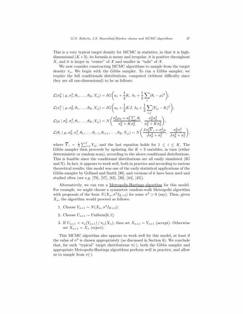
We now consider constructing MCMC algorithms to sample from the targetdensity πu. We begin with the Gibbs sampler. To run a Gibbs sampler, werequire the full conditionals distributions, computed (without difficulty sincethey are all one-dimensional) to be as follows:

L(σ2θ | µ, σ2

e , θ1, . . . , θK , Yij) = IG

(

a1 +1

2K, b1 +

1

2

∑

i

(θi − µ)2)

;

L(σ2e | µ, σ2

θ , θ1, . . . , θK , Yij) = IG

(

a2 +1

2KJ, b2 +

1

2

∑

i,j

(Yij − θi)2

)

;

L(µ | σ2θ , σ2

e , θ1, . . . , θK , Yij) = N

(

σ2θµ0 + σ2

0

∑

i θi

σ2θ + Kσ2

0

,σ2

θσ20

σ2θ + Kσ2

0

)

;

L(θi | µ, σ2θ , σ2

e , θ1, . . . , θi−1, θi+1, . . . , θK , Yij) = N

(

Jσ2θY i + σ2

eµ

Jσ2θ + σ2

e

,σ2

θσ2e

Jσ2θ + σ2

e

)

,

where Y i = 1J

∑Jj=1 Yij , and the last equation holds for 1 ≤ i ≤ K. The

Gibbs sampler then proceeds by updating the K + 3 variables, in turn (eitherdeterministic or random scan), according to the above conditional distributions.This is feasible since the conditional distributions are all easily simulated (IGand N). In fact, it appears to work well, both in practice and according to varioustheoretical results; this model was one of the early statistical applications of theGibbs sampler by Gelfand and Smith [30], and versions of it have been used andstudied often (see e.g. [79], [57], [82], [20], [44], [45]).

Alternatively, we can run a Metropolis-Hastings algorithm for this model.For example, we might choose a symmetric random-walk Metropolis algorithmwith proposals of the form N(Xn, σ2IK+3) for some σ2 > 0 (say). Then, givenXn, the algorithm would proceed as follows:

1. Choose Yn+1 ∼ N(Xn, σ2IK+3);

2. Choose Un+1 ∼ Uniform[0, 1];

3. If Un+1 < πu(Yn+1) / πu(Xn), then set Xn+1 = Yn+1 (accept). Otherwiseset Xn+1 = Xn (reject).

This MCMC algorithm also appears to work well for this model, at least ifthe value of σ2 is chosen appropriately (as discussed in Section 6). We concludethat, for such “typical” target distributions π(·), both the Gibbs sampler andappropriate Metropolis-Hastings algorithms perform well in practice, and allowus to sample from π(·).


3. Bounds on Markov Chain Convergence Times

Once we know how to construct (and run) lots of different MCMC algorithms,other questions arise. Most obviously, do they converge to the distribution π(·)?And, how quickly does this convergence take place?

To proceed, write Pn(x, A) for the n-step transition law of the Markov chain:

Pn(x, A) = P[Xn ∈ A | X0 = x].

The main MCMC convergence questions are, is Pn(x, A) “close” to π(A) forlarge enough n? And, how large is large enough?

3.1. Total Variation Distance

We shall measure the distance to stationary in terms of total variation distance,defined as follows:

Definition. The total variation distance between two probability measures ν1(·)and ν2(·) is:

‖ν1(·) − ν2(·)‖ = supA

|ν1(A) − ν2(A)|.

We can then ask, is limn→∞ ‖Pn(x, ·) − π(·)‖ = 0? And, given ǫ > 0, howlarge must n be so that ‖Pn(x, ·)−π(·)‖ < ǫ? We consider such questions herein.

We first pause to note some simple properties of total variation distance.

Proposition 3. (a) ‖ν1(·) − ν2(·)‖ = supf :X→[0,1] |∫

fdν1 −∫

fdν2|.(b) ‖ν1(·) − ν2(·)‖ = 1

b−a supf :X→[a,b] |∫

fdν1 −∫

fdν2| for any a < b, and in

particular ‖ν1(·) − ν2(·)‖ = 12 supf :X→[−1,1] |

∫

fdν1 −∫

fdν2|.(c) If π(·) is stationary for a Markov chain kernel P , then ‖Pn(x, ·) − π(·)‖ isnon-increasing in n, i.e. ‖Pn(x, ·) − π(·)‖ ≤ ‖Pn−1(x, ·) − π(·)‖ for n ∈ N.(d) More generally, letting (νiP )(A) =

∫

νi(dx)P (x, A), we always have ‖(ν1P )(·)−(ν2P )(·)‖ ≤ ‖ν1(·) − ν2(·)‖.(e) Let t(n) = 2 supx∈X ‖Pn(x, ·) − π(·)‖, where π(·) is stationary. Then t issub-multiplicative, i.e. t(m + n) ≤ t(m) t(n) for m, n ∈ N.(f) If µ(·) and ν(·) have densities g and h, respectively, with respect to someσ-finite measure ρ(·), and M = max(g, h) and m = min(g, h), then

‖µ(·) − ν(·)‖ =1

2

∫

X(M − m) dρ = 1 −

∫

Xm dρ.

(g) Given probability measures µ(·) and ν(·), there are jointly defined randomvariables X and Y such that X ∼ µ(·), Y ∼ ν(·), and P[X = Y ] = 1 − ‖µ(·) −ν(·)‖.


Proof. For (a), let ρ(·) be any σ-finite measure such that ν1 ≪ ρ and ν2 ≪ ρ(e.g. ρ = ν1+ν2), and set g = dν1/dρ and h = dν2/dρ. Then |

∫

fdν1−∫

fdν2| =|∫

f(g − h) dρ|. This is maximised (over all 0 ≤ f ≤ 1) when f = 1 on {g > h}and f = 0 on {h > g} (or vice-versa), in which case it equals |ν1(A) − ν2(A)|for A = {g > h} (or {g < h}), thus proving the equivalence.

Part (b) follows very similarly to (a), except now f = b on {g > h} and f = aon {g < h} (or vice-versa), leading to |

∫

fdν1−∫

fdν2| = (b−a) |ν1(A)−ν2(A)|.For part (c), we compute that

|Pn+1(x, A) − π(A)| =

∣

∣

∣

∣

∫

y∈XPn(x, dy)P (y, A) −

∫

y∈Xπ(dy)P (y, A)

∣

∣

∣

∣

=

∣

∣

∣

∣

∫

y∈XPn(x, dy)f(y) −

∫

y∈Xπ(dy)f(y)

∣

∣

∣

∣

≤ ‖Pn(x, ·) − π(·)‖,

where f(y) = P (y, A), and where the inequality comes from part (a).Part (d) follows very similarly to part (c).Part (e) follows since t(n) is an L∞ operator norm of Pn (cf. Meyn and

Tweedie [54], Lemma 16.1.1). More specifically, let P (x, ·) = Pn(x, ·)−π(·) andQ(x, ·) = Pm(x, ·) − π(·), so that

(P Qf)(x) ≡∫

y∈Xf(y)

∫

z∈X[Pn(x, dz) − π(dz)] [Pm(z, dy) − π(dy)]

=

∫

y∈Xf(y) [Pn+m(x, dy) − π(dy) − π(dy) + π(dy)]

=

∫

y∈Xf(y) [Pn+m(x, dy) − π(dy)].

Then let f : X → [0, 1], let g(x) = (Qf)(x) ≡∫

y∈X Q(x, dy)f(y), and let

g∗ = supx∈X |g(x)|. Then g∗ ≤ 12 t(m) by part (a). Now, if g∗ = 0, then clearly

P Qf = 0. Otherwise, we compute that

2 supx∈X

|(P Qf)(x)| = 2 g∗ supx∈X

|(P [g/g∗])(x)| ≤ t(m) supx∈X

(P [g/g∗])(x)|. (5)

Since −1 ≤ g/g∗ ≤ 1, we have (P [g/g∗])(x) ≤ 2 ‖Pn(x, ·)−π(·)‖ by part (b), sothat supx∈X (P [g/g∗])(x) ≤ t(n). The result then follows from part (a) togetherwith (5).

The first equality of part (f) follows since, as in the proof of part (b) witha = −1 and b = 1, we have

‖µ(·) − ν(·)‖ =1

2

(

∫

g>h

(g − h) dρ +

∫

h>g

(h − g) dρ)

=1

2

∫

X(M − m) dρ.

The second equality of part (f) then follows since M + m = g + h, so that∫

X (M + m) dρ = 2, and hence


1

2

∫

X(M − m) dρ = 1 − 1

2

(

2 −∫

X(M − m) dρ

)

= 1 − 1

2

∫

X

(

(M + m) − (M − m))

dρ = 1 −∫

Xm dρ.

For part (g), we let a =∫

X m dρ, b =∫

X (g − m) dρ, and c =∫

X (h − m) dρ.The statement is trivial if any of a, b, c equal zero, so assume they are all positive.We then jointly construct random variables Z, U, V, I such that Z has densitym/a, U has density (g − m)/b, V has density (h − m)/b, and I is independentof Z, U, V with P[I = 1] = a and P[I = 0] = 1 − a. We then let X = Y = Z ifI = 1, and X = U and Y = V if I = 0. Then it is easily checked that X ∼ µ(·)and Y ∼ ν(·). Furthermore U and V have disjoint support, so P[U = V ] = 0.Then using part (f),

P[X = Y ] = P[I = 1] = a = 1 − ‖µ(·) − ν(·)‖,

as claimed.

Remark. Proposition 3(e) is false without the factor of 2. For example, supposeX = {1, 2}, with P (1, {1}) = 0.3, P (1, {2}) = 0.7, P (2, {1}) = 0.4, P (2, {2}) =0.6, π(1) = 4

11 , and π(2) = 711 . Then π(·) is stationary, and supx∈X ‖P (x, ·) −

π(·)‖ = 0.0636, and supx∈X ‖P 2(x, ·)−π(·)‖ = 0.00636, but 0.00636 > (0.0636)2.On the other hand, some authors instead define total variation distance as twicethe value used here, in which case the factor of 2 in Proposition 3(e) is notwritten explicitly.

3.2. Asymptotic Convergence

Even if a Markov chain has stationary distribution π(·), it may still fail toconverge to stationarity:

Example 1. Suppose X = {1, 2, 3}, with π{1} = π{2} = π{3} = 1/3. LetP (1, {1}) = P (1, {2}) = P (2, {1}) = P (2, {2}) = 1/2, and P (3, {3}) = 1.Then π(·) is stationary. However, if X0 = 1, then Xn ∈ {1, 2} for all n, soP (Xn = 3) = 0 for all n, so P (Xn = 3) 6→ π{3}, and the distribution of Xn doesnot converge to π(·). (In fact, here the stationary distribution is not unique, andthe distribution of Xn converges to a different stationary distribution definedby π{1} = π{2} = 1/2.)

The above example is “reducible”, in that the chain can never get from state 1to state 3, in any number of steps. Now, the classical notion of “irreducibility” isthat the chain has positive probability of eventually reaching any state from anyother state, but if X is uncountable then that condition is impossible. Instead,we demand the weaker condition of φ-irreducibility:


Definition. A chain is φ-irreducible if there exists a non-zero σ-finite measureφ on X such that for all A ⊆ X with φ(A) > 0, and for all x ∈ X , there existsa positive integer n = n(x, A) such that Pn(x, A) > 0.

For example, if φ(A) = δx∗(A), then this requires that x∗ has positive prob-

ability of eventually being reached from any state x. Thus, if a chain has anyone state which is reachable from anywhere (which on a finite state space isequivalent to being indecomposible), then it is φ-irreducible. However, if X isuncountable then often P (x, {y}) = 0 for all x and y. In that case, φ(·) mightinstead be e.g. Lebesgue measure on Rd, so that φ({x}) = 0 for all singletonsets, but such that all subsets A of positive Lebesgue measure are eventuallyreachable with positive probability from any x ∈ X .

Running Example. Here we introduce a running example, to which we shallreturn several times. Suppose that π(·) is a probability measure having unnor-malised density function πu with respect to d-dimensional Lebesgue measure.Consider the Metropolis-Hastings algorithm for πu with proposal density q(x, ·)with respect to d-dimensional Lebesgue measure. Then if q(·, ·) is positive andcontinuous on Rd × Rd, and πu is finite everywhere, then the algorithm is π-irreducible. Indeed, let π(A) > 0. Then there exists R > 0 such that π(AR) > 0,where AR = A∩BR(0), and BR(0) represents the ball of radius R centred at 0.Then by continuity, for any x ∈ Rd, infy∈AR

min{q(x,y), q(y,x)} ≥ ǫ for someǫ > 0, and thus we have (assuming πu(x) > 0, otherwise P (x, A) > 0 followsimmediately) that

P (x, A) ≥ P (x, AR) ≥∫

AR

q(x,y) min

[

1,πu(y) q(y,x)

πu(x) q(x,y)

]

dy

≥ ǫ Leb(

{y ∈ AR : πu(y) ≥ πu(x)})

+ǫ K

πu(x)π(

{y ∈ AR : πu(y) < πu(x)})

,

where K =∫

X πu(x) dx > 0. Since π(·) is absolutely continuous with respect toLebesgue measure, and since Leb(AR) > 0, it follows that the terms in this finalsum cannot both be 0, so that we must have P (x, A) > 0. Hence, the chain isπ-irreducible.

Even φ-irreducible chains might not converge in distribution, due to period-icity problems, as in the following simple example.

Example 2. Suppose again X = {1, 2, 3}, with π{1} = π{2} = π{3} = 1/3.Let P (1, {2}) = P (2, {3}) = P (3, {1}) = 1. Then π(·) is stationary, and thechain is φ-irreducible [e.g. with φ(·) = δ1(·)]. However, if X0 = 1 (say), thenXn = 1 whenever n is a multiple of 3, so P (Xn = 1) oscillates between 0 and 1,so again P (Xn = 1) 6→ π{3}, and there is again no convergence to π(·).

To avoid this problem, we require aperiodicity, and we adopt the followingdefinition (which suffices for the φ-irreducible chains with stationary distribu-tions that we shall study; for more general relationships see e.g. Meyn andTweedie [54], Theorem 5.4.4):


Definition. A Markov chain with stationary distribution π(·) is aperiodic ifthere do not exist d ≥ 2 and disjoint subsets X1,X2, . . . ,Xd ⊆ X withP (x,Xi+1) = 1 for all x ∈ Xi (1 ≤ i ≤ d − 1), and P (x,X1) = 1 for allx ∈ Xd, such that π(X1) > 0 (and hence π(Xi) > 0 for all i). (Otherwise, thechain is periodic, with period d, and periodic decomposition X1, . . . ,Xd.)

Running Example, Continued. Here we return to the Running Example in-troduced above, and demonstrate that no additional assumptions are necessaryto ensure aperiodicity. To see this, suppose that X1 and X2 are disjoint subsetsof X both of positive π measure, with P (x,X2) = 1 for all x ∈ X1. But just takeany x ∈ X1, then since X1 must have positive Lebesgue measure,

P (x,X1) ≥∫

y∈X1

q(x,y)α(x,y) dy > 0

for a contradiction. Therefore aperiodicity must hold. (It is possible to demon-strate similar results for other MCMC algorithms, such as the Gibbs sampler, seee.g. Tierney [93]. Indeed, it is rather rare for MCMC algorithms to be periodic.)

Now we can state the main asymptotic convergence theorem, whose proof isdescribed in Section 4. (This theorem assumes that the state space’s σ-algebrais countably generated, but this is a very weak assumption which is true for e.g.any countable state space, or any subset of Rd with the usual Borel σ-algebra,since that σ-algebra is generated by the balls with rational centers and rationalradii.)

Theorem 4. If a Markov chain on a state space with countably generated σ-algebra is φ-irreducible and aperiodic, and has a stationary distribution π(·),then for π-a.e. x ∈ X ,

limn→∞

‖Pn(x, ·) − π(·)‖ = 0.

In particular, limn→∞ Pn(x, A) = π(A) for all measurable A ⊆ X .

Fact 5. In fact, under the conditions of Theorem 4, if h : X → R withπ(|h|) < ∞, then a “strong law of large numbers” also holds (see e.g. Meynand Tweedie [54], Theorem 17.0.1), as follows:

limn→∞

(1/n)

n∑

i=1

h(Xi) = π(h) w.p. 1. (6)

Theorem 4 requires that the chain be φ-irreducible and aperiodic, and havestationary distribution π(·). Now, MCMC algorithms are created precisely sothat π(·) is stationary, so this requirement is not a problem. Furthermore, itis usually straightforward to verify that chain is φ-irreducible, where e.g. φ isLebesgue measure on an appropriate region. Also, aperiodicity almost always


holds, e.g. for virtually any Metropolis algorithm or Gibbs sampler. Hence, The-orem 4 is widely applicable to MCMC algorithms.

It is worth asking why the convergence in Theorem 4 is just from π-a.e.x ∈ X . The problem is that the chain may have unpredictable behaviour on a“null set” of π-measure 0, and fail to converge there. Here is a simple exampledue to C. Geyer (personal communication):

Example 3. Let X = {1, 2, . . .}. Let P (1, {1}) = 1, and for x ≥ 2, P (x, {1}) =1/x2 and P (x, {x + 1}) = 1 − (1/x2). Then chain has stationary distributionπ(·) = δ1(·), and it is π-irreducible and aperiodic. On the other hand, if X0 =x ≥ 2, then P[Xn = x+n for all n] =

∏∞j=x(1− (1/j2)) > 0, so that ‖Pn(x, ·)−

π(·)‖ 6→ 0. Here Theorem 4 holds for x = 1 which is indeed π-a.e. x ∈ X , but itdoes not hold for x ≥ 2.

Remark. The transient behaviour of the chain on the null set in Example 3is not accidental. If instead the chain converged on the null set to some otherstationary distribution, but still had positive probability of escaping the nullset (as it must to be φ-irreducible), then with probability 1 the chain wouldeventually exit the null set, and would thus converge to π(·) from the null setafter all.

It is reasonable to ask under what circumstances the conclusions of The-orem 4 will hold for all x ∈ X , not just π-a.e. Obviously, this will hold ifthe transition kernels P (x, ·) are all absolutely continuous with respect to π(·)(i.e., P (x, dy) = p(x, y)π(dy) for some function p : X ×X → [0,∞)), or for anyMetropolis algorithm whose proposal distributions Q(x, ·) are absolutely contin-uous with respect to π(·). It is also easy to see that this will hold for our RunningExample described above. More generally, it suffices that the chain be Harris re-current, meaning that for all B ⊆ X with π(B) > 0, and all x ∈ X , the chain willeventually reach B from x with probability 1, i.e. P[∃n : Xn ∈ B |X0 = x] = 1.This condition is stronger than π-irreducibility (as evidenced by Example 3); forfurther discussions of this see e.g. Orey [61], Tierney [93], Chan and Geyer [15],and [75].

Finally, we note that periodic chains occasionally arise in MCMC (see e.g.Neal [58]), and much of the theory can be applied to this case. For example, wehave the following.

Corollary 6. If a Markov chain is φ-irreducible, with period d ≥ 2, and has astationary distribution π(·), then for π-a.e. x ∈ X ,

limn→∞

∥

∥

∥(1/d)

n+d−1∑

i=n

P i(x, ·) − π(·)∥

∥

∥= 0, (7)

and also the strong law of large numbers (6) continues to hold without change.


Proof. Let the chain have periodic decomposition X1, . . . ,Xd ⊆ X , and letP ′ be the d-step chain P d restricted to the state space X1. Then P ′ is φ-irreducible and aperiodic on X1, with stationary distribution π′(·) which sat-

isfies that π(·) = (1/d)∑d−1

j=0 (π′ P j)(·). Now, from Proposition 3(c), it sufficesto prove the Corollary when n = md with m → ∞, and for simplicity we as-sume without loss of generality that x ∈ X1. From Proposition 3(d), we have‖Pmd+j(x, ·)− (π′ P j)(·)‖ ≤ ‖Pmd(x, ·)−π′(·)‖ for j ∈ N. Then, by the triangleinequality,

∥

∥

∥(1/d)

md+d−1∑

i=md

P i(x, ·) − π(·)∥

∥

∥=∥

∥

∥(1/d)

d−1∑

j=0

Pmd+j(x, ·) − (1/d)

d−1∑

j=0

(π′ P j)(·)∥

∥

∥

≤ (1/d)

d−1∑

j=0

‖Pmd+j(x, ·) − (π′ P j)(·)‖ ≤ (1/d)

d−1∑

j=0

‖Pmd(x, ·) − π′(·)‖.

But applying Theorem 4 to P ′, we obtain that limm→∞ ‖Pmd(x, ·)− π′(·)‖ = 0for π′-a.e. x ∈ X1, thus giving the first result.

To establish (6), let P be the transition kernel for the Markov chain onX1× . . .×Xd corresponding to the sequence {(Xmd, Xmd+1, . . . , Xmd+d−1)}∞m=0,and let h(x0, . . . , xd−1) = (1/d)(h(x0) + . . . + h(xd−1)). Then just like P ′, wesee that P is φ-irreducible and aperiodic, with stationary distribution given by

π = π′ × (π′P ) × (π′P 2) × . . . × (π′P d−1).

Applying Fact 5 to P and h establishes that (6) holds without change.

Remark. By similar methods, it follows that (5) also remains true in the peri-odic case, i.e. that

limn→∞

(1/n)

n∑

i=1

h(Xi) = π(h) w.p. 1

whenever h : X → R with π(|h|) < ∞, provided the Markov chain is φ-irreducible and countably generated, without any assumption of aperiodicity.In particular, both (7) and (5) hold (without further assumptions re period-icity) for any irreducible (or indecomposible) Markov chain on a finite statespace.

A related question for periodic chains, not considered here, is to considerquantitative bounds on the difference of average distributions,

∥

∥

∥

∥

∥

(1/n)

n∑

i=1

P i(x, ·) − π(·)∥

∥

∥

∥

∥

,

through the use of shift-coupling; see Aldous and Thorisson [3], and [68].


3.3. Uniform Ergodicity

Theorem 4 implies asymptotic convergence to stationarity, but does not sayanything about the rate of this convergence. One “qualitative” convergence rateproperty is uniform ergodicity:

Definition. A Markov chain having stationary distribution π(·) is uniformlyergodic if

‖Pn(x, ·) − π(·)‖ ≤ M ρn, n = 1, 2, 3, . . .

for some ρ < 1 and M < ∞.

One equivalence of uniform ergodicity is:

Proposition 7. A Markov chain with stationary distribution π(·) is uniformlyergodic if and only if supx∈X ‖Pn(x, ·) − π(·)‖ < 1/2 for some n ∈ N.

Proof. If the chain is uniformly ergodic, then

limn→∞

supx∈X

‖Pn(x, ·) − π(·)‖ ≤ limn→∞

M ρn = 0,

so supx∈X ‖Pn(x, ·) − π(·)‖ < 1/2 for all sufficiently large n. Conversely, ifsupx∈X ‖Pn(x, ·) − π(·)‖ < 1/2 for some n ∈ N, then in the notation of Propo-

sition 3(e), we have that d(n) ≡ β < 1, so that for all j ∈ N, d(jn) ≤(

d(n))j

=βj . Hence, from Proposition 3(c),

‖Pm(x, ·) − π(·)‖ ≤ ‖P ⌊m/n⌋n(x, ·) − π(·)‖ ≤ 1

2d (⌊m/n⌋n)

≤ β⌊m/n⌋ ≤ β−1(

β1/n)m

,

so the chain is uniformly ergodic with M = β−1 and ρ = β1/n.

Remark. The above Proposition of course continues to hold if we replace 1/2by δ for any 0 < δ < 1/2. However, it is false for δ ≥ 1/2. For example, ifX = {1, 2}, with P (1, {1}) = P (2, {2}) = 1, and π(·) is uniform on X , then‖Pn(x, ·) − π(·)‖ = 1/2 for all x ∈ X and n ∈ N.

To develop further conditions which ensure uniform ergodicity, we require adefinition.

Definition. A subset C ⊆ X is small (or, (n0, ǫ, ν)-small) if there exists apositive integer n0, ǫ > 0, and a probability measure ν(·) on X such that thefollowing minorisation condition holds:

Pn0(x, ·) ≥ ǫ ν(·) x ∈ C, (8)

i.e. Pn0(x, A) ≥ ǫ ν(A) for all x ∈ C and all measurable A ⊆ X .


Remark. Some authors (e.g. Meyn and Tweedie [54]) also require that C havepositive stationary measure, but for simplicity we don’t explicitly require thathere. In any case, π(C) > 0 follows under the additional assumption of the driftcondition (10) considered in the next section.

Intuitively, this condition means that all of the n0-step transitions fromwithin C, all have an “ǫ-overlap”, i.e. a component of size ǫ in common. (Thisconcept goes back to Doeblin [22]; for further background, see e.g. [23], [8], [60],[4], and [54]; for applications to convergence rates see e.g. [55], [80], [82], [71],[77], [24], [85].) We note that if X is countable, and if

ǫn0 ≡∑

y∈Xinfx∈C

Pn0(x, {y}) > 0, (9)

then C is (n0, ǫn0 , ν)-small where ν{y} = ǫ−1n0

infx∈C Pn0(x, {y}). (Furthermore,for an irreducible (or just indecomposible) and aperiodic chain on a finite statespace, we always have ǫn0 > 0 for sufficiently large n0 (see e.g. [81]), so thismethod always applies in principle.) Similarly, if the transition probabilities havedensities with respect to some measure η(·), i.e. if Pn0(x, dy) = pn0(x, y) η(dy),then we can take ǫn0 =

∫

y∈X(

infx∈X pn0(x, y))

η(dy).

Remark. As observed in [72], small-set conditions of the form P (x, ·) ≥ ǫ ν(·)for all x ∈ C, can be replaced by pseudo-small conditions of the form P (x, ·) ≥ǫ νxy(·) and P (y, ·) ≥ ǫ νxy(·) for all x, y ∈ C, without affecting any bounds whichuse pairwise coupling (which includes all of the bounds considered here beforeSection 5. Thus, all of the results stated in this section remain true withoutchange if “small set” is replaced by “pseudo-small set” in the hypotheses. Forease of exposition, we do not emphasise this point herein.

The main result guaranteeing uniform ergodicity, which goes back to Doe-blin [22] and Doob [23] and in some sense even to Markov [50], is the following.

Theorem 8. Consider a Markov chain with invariant probability distributionπ(·). Suppose the minorisation condition (8) is satisfied for some n0 ∈ N andǫ > 0 and probability measure ν(·), in the special case C = X (i.e., the en-tire state space is small). Then the chain is uniformly ergodic, and in fact‖Pn(x, ·) − π(·)‖ ≤ (1 − ǫ)⌊n/n0⌋ for all x ∈ X , where ⌊r⌋ is the greatest in-teger not exceeding r.

Theorem 8 is proved in Section 4. We note also that Theorem 8 providesa quantitative bound on the distance to stationarity ‖Pn(x, ·) − π(·)‖, namelythat it must be ≤ (1− ǫ)⌊n/n0⌋. Thus, once n0 and ǫ are known, we can find n∗such that, say, ‖Pn∗(x, ·) − π(·)‖ ≤ 0.01, a fact which can be applied in certainMCMC contexts (see e.g. [78]). We can then say that n∗ iterations “sufficesfor convergence” of the Markov chain. On a discrete state space, we have that‖Pn(x, ·) − π(·)‖ ≤ (1 − ǫn0)

⌊n/n0⌋ with ǫn0 as in (9).


Running Example, Continued. Recall our Running Example, introducedabove. Since we have imposed strong continuity conditions on q, it is natural toconjecture that compact sets are small. However this is not true without extraregularity conditions. For instance, consider dimension d = 1, and suppose thatπu(x) = 10<|x|<1|x|−1/2, and let q(x, y) ∝ exp{−(x − y)2/2}, then it is easy tocheck that any neighbourhood of 0 is not small. However in the general setupof our Running Example, all compact sets on which πu is bounded are small.To see this, suppose C is a compact set on which πu is bounded by k < ∞. Letx ∈ C, and let D be any compact set of positive Lebesgue and π measure, suchthat infx∈C,y∈D q(x,y) = ǫ > 0 for all y ∈ D. We then have,

P (x, dy) ≥ q(x,y) dy min

{

1,πu(y)

πu(x)

}

≥ ǫ dymin

{

1,πu(y)

k

}

,

which is a positive measure independent of x. Hence, C is small. (This examplealso shows that if πu is continuous, the state space X is compact, and q iscontinuous and positive, then X is small, and so the chain must be uniformlyergodic.)

If a Markov chain is not uniformly ergodic (as few MCMC algorithms onunbounded state spaces are), then Theorem 8 cannot be applied. However, itis still of great importance, given a Markov chain kernel P and an initial statex, to be able to find n∗ so that, say, ‖Pn∗(x, ·) − π(·)‖ ≤ 0.01. This issue isdiscussed further below.

3.4. Geometric ergodicity

A weaker condition than uniform ergodicity is geometric ergodicity, as follows(for background and history, see e.g. Nummelin [60], and Meyn and Tweedie [54]):

Definition. A Markov chain with stationary distribution π(·) is geometricallyergodic if

‖Pn(x, ·) − π(·)‖ ≤ M(x) ρn, n = 1, 2, 3, . . .

for some ρ < 1, where M(x) < ∞ for π-a.e. x ∈ X .

The difference between geometric ergodicity and uniform ergodicity is thatnow the constant M may depend on the initial state x.

Of course, if the state space X is finite, then all irreducible and aperi-odic Markov chains are geometrically (in fact, uniformly) ergodic. However,for infinite X this is not the case. For example, it is shown by Mengersen andTweedie [52] (see also [76]) that a symmetric random-walk Metropolis algorithmis geometrically ergodic essentially if and only if π(·) has finite exponential mo-ments. (For chains which are not geometrically ergodic, it is possible also tostudy polynomial ergodicity, not considered here; see Fort and Moulines [29],and Jarner and Roberts [42].) Hence, we now discuss conditions which ensuregeometric ergodicity.


Definition. Given Markov chain transition probabilities P on a state space X ,and a measurable function f : X → R, define the function Pf : X → R suchthat (Pf)(x) is the conditional expected value of f(Xn+1), given that Xn = x.In symbols, (Pf)(x) =

∫

y∈X f(y)P (x, dy).

Definition. A Markov chain satisfies a drift condition (or, univariate geometricdrift condition) if there are constants 0 < λ < 1 and b < ∞, and a functionV : X → [1,∞], such that

PV ≤ λV + b1C , (10)

i.e. such that∫

X P (x, dy)V (y) ≤ λV (x) + b1C(x) for all x ∈ X .

The main result guaranteeing geometric ergodicity is the following.

Theorem 9. Consider a φ-irreducible, aperiodic Markov chain with stationarydistribution π(·). Suppose the minorisation condition (8) is satisfied for someC ⊂ X and ǫ > 0 and probability measure ν(·). Suppose further that the driftcondition (10) is satisfied for some constants 0 < λ < 1 and b < ∞ , and afunction V : X → [1,∞] with V (x) < ∞ for at least one (and hence for π-a.e.)x ∈ X . Then then chain is geometrically ergodic.

Theorem 9 is usually proved by complicated analytic arguments (see e.g. [60],[54], [7]). In Section 4, we describe a proof of Theorem 9 which uses direct cou-pling constructions instead. Note also that Theorem 9 provides no quantitativebounds on M(x) or ρ, though this is remedied in Theorem 12 below.

Fact 10. In fact, it follows from Theorems 15.0.1, 16.0.1, and 14.3.7 of Meynand Tweedie [54], and Proposition 1 of [69], that the minorisation condition (8)and drift condition (10) of Theorem 9 are equivalent (assuming φ-irreducibilityand aperiodicity) to the apparently stronger property of “V -uniform ergodicity”,i.e. that there is C < ∞ and ρ < 1 such that

sup|f |≤V

|Pnf(x) − π(f)| ≤ C V (x) ρn, x ∈ X ,

where π(f) =∫

x∈X f(x)π(dx). That is, we can take sup|f |≤V instead of justsup0<f<1 (compare Proposition 3 parts (a) and (b)), and we can let M(x) =C V (x) in the geometric ergodicity bound. Furthermore, we always have π(V ) <∞. (The term “V -uniform ergodicity”, as used in [54], perhaps also implies thatV (x) < ∞ for all x ∈ X , rather than just for π-a.e. x ∈ X , though we do notconsider that distinction further here.)


Open Problem # 1. Can direct coupling methods, similar to those used belowto prove Theorem 9, also be used to provide an alternative proof of Fact 10?

Example 4. Here we consider a simple example of geometric ergodicity ofMetropolis algorithms on R (see Mengersen and Tweedie [52], and [76]). Supposethat X = R+ and πu(x) = e−x. We will use a symmetric (about x) proposaldistribution q(x, y) = q(|y − x|) with support contained in [x− a, x + a]. In thissimple situation, a natural drift function to take is V (x) = ecx for some c > 0.For x ≥ a, we compute:

PV (x) =

∫ x

x−a

V (y)q(x, y)dy +

∫ x+a

x

V (y)q(x, y)dyπu(y)

πu(x)

+ V (x)

∫ x+a

x

q(x, y)dy(1 − πu(y)/πu(x)).

By the symmetry of q, this can be written as

∫ x+a

x

I(x, y) q(x, y) dy,

where

I(x, y) =V (y)πu(y)

πu(x)+ V (2x − y) + V (x)

(

1 − πu(y)

πu(x)

)

= ecx[

e(c−1)u + e−cu + 1 − e−u]

= ecx[

2 − (1 + e(c−1)u)(1 − e−cu)]

,

and where u = y − x. For c < 1, this is equal to 2(1 − ǫ)V (x) for some positiveconstant ǫ. Thus in this case we have shown that for all x > a

PV (x) ≤∫ x+a

x

2V (x)(1 − ǫ)q(x, y)dy = (1 − ǫ)V (x).

Furthermore, it is easy to show that PV (x) is bounded on [0, a] and that [0, a]is in fact a small set. Thus, we have demonstrated that the drift condition (10)holds. Hence, the algorithm is geometrically ergodic by Theorem 9. (It turnsout that for such Metropolis algorithms, a certain condition, which essentiallyrequires an exponential bound on the tail probabilities of π(·), is in fact necessaryfor geometric ergodicity; see [76].)

Implications of geometric ergodicity for central limit theorems are discussedin Section 5. In general, it believed by practitioners of MCMC that geometricergodicity is a useful property. But does geometric ergodicity really matter?Consider the following examples.


Example 5. ([71]) Consider an independence sampler, with π(·) an Expo-nential(1) distribution, and Q(x, ·) an Exponential(λ) distribution. Then if 0 <λ ≤ 1, the sampler is geometrically ergodic, has central limit theorems (seeSection 5), and generally behaves fairly well even for very small λ. On the otherhand, for λ > 1 the sampler fails to be geometrically ergodic, and indeed forλ ≥ 2 it fails to have central limit theorems, and generally behaves quite poorly.For example, the simulations in [71] indicate that with λ = 5, when startedin stationarity and averaged over the first million iterations, the sampler willusually return an average value of about 0.8 instead of 1, and then occasionallyreturn a very large value instead, leading to very unstable behaviour. Thus, thisis an example where the property of geometric ergodicity does indeed correspondto stable, useful convergence behaviour.

However, geometric ergodicity does not always guarantee a useful Markovchain algorithm, as the following two examples show.

Example 6. (“Witch’s Hat”, e.g. Matthews [51]) Let X = [0, 1], let δ = 10−100

(say), let 0 < a < 1 − δ, and let πu(x) = δ + 1[a,a+δ](x). Then π([a, a +δ]) ≈ 1/2. Now, consider running a typical Metropolis algorithm on πu. UnlessX0 ∈ [a, a + δ], or the sampler gets “lucky” and achieves Xn ∈ [a, a + δ] forsome moderate n, then the algorithm will likely miss the tiny interval [a, a + δ]entirely, over any feasible time period. The algorithm will thus “appear” (to thenaked eye or to any statistical test) to converge to the Uniform(X ) distribution,even though Uniform(X ) is very different from π(·). Nevertheless, this algorithmis still geometrically ergodic (in fact uniformly ergodic). So in this example,geometric ergodicity does not guarantee a well-behaved sampler.

Example 7. Let X = R, and let πu(x) = 1/(1 + x2) be the (unnormalised)density of the Cauchy distribution. Then a random-walk Metropolis algorithmfor πu (with, say, X0 = 0 and Q(x, ·) = Uniform[x−1, x+1]) is ergodic but is notgeometrically ergodic. And, indeed, this sampler has very slow, poor convergenceproperties. On the other hand, let π′

u(x) = πu(x)1|x|≤10100 , i.e. π′u corresponds

to πu truncated at ± one googol. Then the same random-walk Metropolis algo-rithm for π′

u is geometrically ergodic, in fact uniformly ergodic. However, thetwo algorithms are indistinguishable when run for any remotely feasible numberof iterations. Thus, this is an example where geometric ergodicity does not inany way indicate improved performance of the algorithm.

In addition to the above two examples, there are also numerous examplesof important Markov chains on finite state spaces (such as the single-site Gibbssampler for the Ising model at low temperature on a large but finite grid) whichare irreducible and aperiodic, and hence uniformly (and thus also geometrically)ergodic, but which converge to stationarity extremely slowly.

The above examples illustrate a limitation of qualitative convergence prop-erties such as geometric ergodicity. It is thus desirable where possible to insteadobtain quantitative bounds on Markov chain convergence. We consider this issuenext.


3.5. Quantitative Convergence Rates

In light of the above, we ideally want quantitative bounds on convergence rates,i.e. bounds of the form ‖Pn(x, ·) − π(·)‖ ≤ g(x, n) for some explicit functiong(x, n), which (hopefully) is small for large n. Such questions now have a sub-stantial history in MCMC, see e.g. [55], [80], [82], [49], [20], [77], [44], [45], [24],[11], [85], [28], [9], [86], [87].

We here present a result from [85], which follows as a special case of [24]; it isbased on the approach of [80] while also taking into account a small improvementfrom [77].

Our result requires a bivariate drift condition of the form

Ph(x, y) ≤ h(x, y)/α, (x, y) /∈ C × C (11)

for some function h : X × X → [1,∞) and some α > 1, where

Ph(x, y) ≡∫

X

∫

Xh(z, w)P (x, dz)P (y, dw).

(Thus, P represents running two independent copies of the chain.) Of course, (11)is closely related to (10); for example we have the following (see also [80], andProposition 2 of [87]):

Proposition 11. Suppose the univariate drift condition (10) is satisfied forsome V : X → [1,∞], C ⊆ X , λ < 1, and b < ∞. Let d = infx∈Cc V (x). Thenif d > [b/(1 − λ)] − 1, then the bivariate drift condition (11) is satisfied for thesame C, with h(x, y) = 1

2 [V (x) + V (y)] and α−1 = λ + b/(d + 1) < 1.

Proof. If (x, y) /∈ C × C, then either x /∈ C or y /∈ C (or both), so h(x, y) ≥(1 + d)/2, and PV (x) + PV (y) ≤ λV (x) + λV (y) + b. Then

Ph(x, y) =1

2[PV (x) + PV (y)] ≤ 1

2[λV (x) + λV (y) + b]

= λh(x, y) + b/2 ≤ λh(x, y) + (b/2)[h(x, y)/((1 + d)/2)]

= [λ + b/(1 + d)] h(x, y).

Furthermore, d > [b/(1 − λ)] − 1 implies that λ + b/(1 + d) < 1.

Finally, we let

Bn0 = max

[

1, αn0(1 − ǫ) supC×C

Rh

]

, (12)

where for (x, y) ∈ C × C,

Rh(x, y) =

∫

X

∫

X(1 − ǫ)−2h(z, w) (Pn0(x, dz) − ǫν(dz)) (Pn0(y, dw) − ǫν(dw)).

In terms of these assumptions, we state our result as follows.


Theorem 12. Consider a Markov chain on a state space X , having transitionkernel P . Suppose there is C ⊆ X , h : X ×X → [1,∞), a probability distributionν(·) on X , α > 1, n0 ∈ N, and ǫ > 0, such that (8) and (11) hold. Define Bn0

by (12). Then for any joint initial distribution L(X0, X′0), and any integers

1 ≤ j ≤ k, if {Xn} and {X ′n} are two copies of the Markov chain started in the

joint initial distribution L(X0, X′0), then

‖L(Xk) − L(X ′k)‖TV ≤ (1 − ǫ)j + α−k (Bn0)

j−1 E[h(X0, X′0)].

In particular, by choosing j = ⌊rk⌋ for sufficiently small r > 0, we obtain anexplicit, quantitative convergence bound which goes to 0 exponentially quickly ask → ∞.

Theorem 12 is proved in Section 4. Versions of this theorem have been appliedto various realistic MCMC algorithms, including for versions of the variancecomponents model described earlier, resulting in bounds like ‖Pn(x, ·)−π(·)‖ <0.01 for n = 140 or n = 3415; see e.g. [82], and Jones and Hobert [45]. Thus,while it is admittedly hard work to apply Theorem 12 to realistic MCMC al-gorithms, it is indeed possible and often can establish rigorously that perfectlyfeasible numbers of iterations are sufficient to ensure convergence.

Remark. For complicated Markov chains, it might be difficult to apply Theo-rem 12 successfully. In such cases, MCMC practitioners instead use “convergencediagnostics”, i.e. do statistical analysis of the realised output X1, X2, . . ., to seeif the distributions of Xn appear to be “stable” for large enough n. Many suchdiagnostics involve running the Markov chain repeatedly from different initialstates, and checking if the chains all converge to approximately the same dis-tribution (see e.g. Gelman and Rubin [31], and Cowles and Carlin [18]). Thistechnique often works well in practice. However, it provides no rigorous guar-antees and can sometimes be fooled into prematurely claiming convergence (seee.g. [51]), as is likely to happen for the examples at the end of Section 3. Fur-thermore, convergence diagnostics can also introduce bias into the resultingestimates (see [19]). Overall, despite the extensive theory surveyed herein, the“convergence time problem” remains largely unresolved for practical applicationof MCMC. (This is also the motivation for “perfect MCMC” algorithms, orig-inally developed by Propp and Wilson [63] and not discussed here; for furtherdiscussion see e.g. Kendall and Møller [46], Thonnes [92], and Fill et al. [27].)

4. Convergence Proofs using Coupling Constructions

In this section, we prove some of the theorems stated earlier. There are of coursemany methods available for bounding convergence of Markov chains, appropriateto various settings (see e.g. [1], [21], [88], [2], [90], and Subsection 5.4 herein),including the setting of large but finite state spaces that often arises in computerscience (see e.g. Sinclair [88] and Randall [64]) but is not our emphasis here. Inthis section, we focus on the method of coupling, which seems particularly well-suited to analysing MCMC algorithms on general (uncountable) state spaces.It is also particularly well-suited to incorporating small sets (though small sets


can also be combined with regeneration theory, see e.g. [8], [4], [57], [38]). Someof the proofs below are new, and avoid many of the long analytic arguments ofsome previous proofs (e.g. Nummelin [60], and Meyn and Tweedie [54]).

4.1. The Coupling Inequality

The basic idea of coupling is the following. Suppose we have two random vari-ables X and Y , defined jointly on some space X . If we write L(X) and L(Y )for their respective probability distributions, then we can write

‖L(X) − L(Y )‖ = supA

|P (X ∈ A) − P (Y ∈ A)|

= supA

|P (X ∈ A, X = Y ) + P (X ∈ A, X 6= Y )

− P (Y ∈ A, Y = X) − P (Y ∈ A, Y 6= X)|= sup

A|P (X ∈ A, X 6= Y ) − P (Y ∈ A, Y 6= X)|

≤ P (X 6= Y ),

so that‖L(X) − L(Y )‖ ≤ P (X 6= Y ). (13)

That is, the variation distance between the laws of two random variables isbounded by the probability that they are unequal. For background, see e.g.Pitman [62], Lindvall [48], and Thorisson [91].

4.2. Small Sets and Coupling

Suppose now that C is a small set. We shall use the following coupling con-struction, which is essentially the “splitting technique” of Nummelin [59] andAthreya and Ney [8]; see also Nummelin [60], and Meyn and Tweedie [54]. Theidea is to run two copies {Xn} and {X ′

n} of the Markov chain, each of whichmarginally follows the updating rules P (x, ·), but whose joint construction (us-ing C) gives them as high a probability as possible of becoming equal to eachother.

THE COUPLING CONSTRUCTION:Start with X0 = x and X ′

0 ∼ π(·), and n = 0, and repeat the following loopforever.

Beginning of Loop. Given Xn and X ′n:

1. If Xn = X ′n, choose Xn+1 = X ′

n+1 ∼ P (Xn, ·), and replace n by n + 1.

2. Else, if (Xn, X ′n) ∈ C × C, then:

(a) w.p. ǫ, choose Xn+n0 = X ′n+n0

∼ ν(·);(b) else, w.p. 1 − ǫ, conditionally independently choose

Xn+n0 ∼ 1

1 − ǫ[Pn0(Xn, ·) − ǫ ν(·)],


X ′n+n0

∼ 1

1 − ǫ[Pn0(X ′

n, ·) − ǫ ν(·)].

In the case n0 > 1, for completeness go back and construct Xn+1, . . . , Xn+n0−1

from their correct conditional distributions given Xn and Xn+n0 , andsimilarly (and conditionally independently) construct X ′

n+1, . . . , X′n+n0−1

from their correct conditional distributions given X ′n and X ′

n+n0. In any

case, replace n by n + n0.

3. Else, conditionally independently choose Xn+1 ∼ P (Xn, ·) and X ′n+1 ∼

P (X ′n, ·), and replace n by n + 1.

Then return to Beginning of Loop.

Under this construction, it is easily checked that Xn and X ′n are each

marginally updated according to the correct transition kernel P . It follows thatP[Xn ∈ A] = Pn(x, ·) and P[X ′

n ∈ A] = π(A) for all n. Moreover the two chainsare run independently until they both enter C at which time the minorisationsplitting construction (step 2) is utilised. Without such a construction, on un-countable state spaces, we would not be able to ensure successful coupling ofthe two processes.

The coupling inequality then says that ‖Pn(x, ·)−π(·)‖ ≤ P[Xn 6= X ′n]. The

question is, can we use this to obtain useful bounds on ‖Pn(x, ·) − π(·)‖? Infact, we shall now provide proofs (nearly self-contained) of all of the theoremsstated earlier, in terms of this coupling construction. This allows for intuitiveunderstanding of the theorems, while also avoiding various analytic technicalitiesof the previous proofs of some of these theorems.

4.3. Proof of Theorem 8

In this case, C = X , so every n0 iterations we have probability at least ǫ ofmaking Xn and X ′

n equal. It follows that if n = n0m, then P[Xn 6= X ′n] ≤

(1 − ǫ)m. Hence, from the coupling inequality, ‖Pn(x, ·) − π(·)‖ ≤ (1 − ǫ)m =(1 − ǫ)n/n0 in this case. It then follows from Proposition 3(c) that ‖Pn(x, ·) −π(·)‖ ≤ (1 − ǫ)⌊n/n0⌋ for any n.


We follow the general outline of [85]. We again begin by assuming that n0 = 1in the minorisation condition for the small set C (and thus write Bn0 as B),and indicate at the end what changes are required if n0 > 1.

LetNk = #{m : 0 ≤ m ≤ k, (Xm, X ′

m) ∈ C × C},and let τ1, τ2, . . . be the times of the successive visits of {(Xn, X ′

n)} to C × C.Then for any integer j with 1 ≤ j ≤ k,

P[Xk 6= X ′k] = P[Xk 6= X ′

k, Nk−1 ≥ j] + P[Xk 6= X ′k, Nk−1 < j]. (14)


Now, the event {Xk 6= X ′k, Nk−1 ≥ j} is contained in the event that the

first j coin flips all came up tails. Hence, P[Xk 6= X ′k, Nk−1 ≥ j] ≤ (1 − ǫ)j .

which bounds the first term in (14).To bound the second term in (14), let

Mk = αkB−Nk−1h(Xk, X ′k)1(Xk 6= X ′

k), k = 0, 1, 2, . . .

(where N−1 = 0).

Lemma 13. We have

E[Mk+1 | X0, . . . , Xk, X ′0, . . . , X

′k] ≤ Mk,

i.e. {Mk} is a supermartingale.

Proof. If (Xk, X ′k) /∈ C × C, then Nk = Nk−1, so

E[Mk+1 | X0, . . . , Xk, X ′0, . . . , X

′k]

= αk+1B−Nk−1E[h(Xk+1, X′k+1)1(Xk+1 6= X ′

k+1) | Xk, X ′k]

(since our coupling construction is Markovian)

≤ αk+1B−Nk−1E[h(Xk+1, X′k+1) | Xk, X ′

k]1(Xk 6= X ′k)

= Mk α E[h(Xk+1, X′k+1) | Xk, X ′

k] / h(Xk, X ′k)

≤ Mk,

by (9). Similarly, if (Xk, X ′k) ∈ C × C, then Nk = Nk−1 + 1, so assuming

Xk 6= X ′k (since if Xk = X ′

k, then the result is trivial), we have

E[Mk+1 | X0, . . . , Xk, X ′0, . . . , X

′k]

= αk+1B−Nk−1−1E[h(Xk+1, X′k+1)1(Xk+1 6= X ′

k+1) | Xk.X ′k]

= αk+1B−Nk−1−1(1 − ǫ)(Rh)(Xk, X ′k)

= MkαB−1(1 − ǫ)(Rh)(Xk, X ′k)/h(Xk, X ′

k)

≤ Mk,

by (10). Hence, {Mk} is a supermartingale.

To proceed, we note that since B ≥ 1,

P[Xk 6= X ′k, Nk−1 < j] = P[Xk 6= X ′

k, Nk−1 ≤ j − 1]

≤ P[Xk 6= X ′k, B−Nk−1 ≥ B−(j−1)]

= P[1(Xk 6= X ′k)B−Nk−1 ≥ B−(j−1)]

≤ Bj−1E[1(Xk 6= X ′k)B−Nk−1 ] (by Markov’s inequality)

≤ Bj−1E[1(Xk 6= X ′k)B−Nk−1 h(Xk, X ′

k)] (since h ≥ 1)

= α−kBj−1E[Mk] (by defn of Mk)

≤ α−kBj−1E[M0] (since {Mk} is supermartingale)

= α−kBj−1E[h(X0, X′0)] (by defn of M0).


Theorem 12 now follows (in the case n0 = 1), by combining these two boundswith (14) and (13).

Finally, we consider the changes required if n0 > 1. In this case, the mainchange is that we do not wish to count visits to C × C during which the jointchain could not try to couple, i.e. visits which correspond to the “filling in”times for going back and constructing Xn+1, . . . , Xn+n0 [and similarly for X ′]in step 2 of the coupling construction. Thus, we instead let Nk count the numberof visits to C × C, and {τi} the actual visit times, avoiding all such “filling in”times. Also, we replace Nk−1 by Nk−n0 in (14) and in the definition of Mk.Finally, what is a supermartingale is not {Mk} but rather {Mt(k)}, where t(k)is the latest time ≤ k which does not correspond to a “filling in” time. (Thus,t(k) will take the value k, unless the joint chain visited C × C at some timebetween k − n0 and k − 1.) With these changes, the proof goes through just asbefore.


Here we give a direct coupling proof of Theorem 9, thereby somewhat avoidingthe technicalities of e.g. Meyn and Tweedie [54] (though admittedly with aslightly weaker conclusion; see Fact 10). Our approach shall be to make use ofTheorem 12. To begin, set h(x, y) = 1

2 [V (x) + V (y)]. Our proof will use thefollowing technical result.

Lemma 14. We may assume without loss of generality that

supx∈C

V (x) < ∞. (15)

Specifically, given a small set C and drift function V satisfying (8) and (10), wecan find a small set C0 ⊆ C such that (8) and (10) still hold (with the same n0

and ǫ and b, but with λ replaced by some λ0 < 1), and such that (15) also holds.

Proof. Let λ and b be as in (10). Choose δ with 0 < δ < 1 − λ, let λ0 = 1 − δ,let K = b/(1 − λ − δ), and set

C0 = C ∩ {x ∈ X : V (x) ≤ K}.

Then clearly (8) continues to hold on C0, since C0 ⊆ C. It remains to verifythat (10) holds with C replaced by C0, and λ replaced by λ0. Now, (10) clearlyholds for x ∈ C0 and x /∈ C, by inspection. Finally, for x ∈ C \ C0, we haveV (x) ≥ K, and so using the original drift condition (10), we have

(PV )(x) ≤ λV (x) + b 1C(x) = (1 − δ)V (x) − (1 − λ − δ)V (x) + b

≤ (1 − δ)V (x) − (1 − λ − δ)K + b = (1 − δ)V (x) = λ0 V (x),

showing that (10) still holds, with C replaced by C0 and λ replaced by λ0.


As an aside, we note that in Lemma 14, it may not be possible to satisfy (15)by instead modifying V and leaving C unchanged:

Proposition 15. There exists a geometrically ergodic Markov chain, with smallset C and drift function V satisfying (8) and (10), such that there does not exista drift function V0 : X → [0,∞] with the property that upon replacing V byV0, (8) and (10) continue to hold, and (15) also holds.

Proof. Consider the Markov chain on X = (0,∞), defined as follows. For x ≥ 2,P (x, ·) = δx−1(·), a point-mass at x − 1. For 1 < x < 2, P (x, ·) is uniformon [1/2, 1]. For 0 < x ≤ 1, P (x, ·) = 1

2 λ(·) + 12 δh(x)(·), where λ is Lebesgue

measure on (0, 1), and h(x) = 1 +√

log(1/x).For this chain, the interval C = (0, 1) is clearly (1, 1/2, λ)-small. Further-

more, since∫ 1

0

√

log(1/x) dx =√

π/2 < ∞, the return times to C have finitemean, so the chain has a stationary distribution by standard renewal theoryarguments (see e.g. Asmussen [4]). In addition, with drift function V (x) =max(ex, x−1/2), we can compute (PV )(x) explicitly, and verify directly that(say) PV (x) ≤ 0.8 V (x) + 4 1C(x) for all x ∈ X , thus verifying (10) withλ = 0.8 and b = 4. Hence, by Theorem 9, the chain is geometrically er-godic.

On the other hand, suppose we had a some drift function V0 satisfying (10),

such that supx∈C V0(x) < ∞. Then since PV0(x) = 12V0(h(x)) + 1

2

∫ 1

0V0(y) dy,

this would imply that supx∈C V0((h(x)) < ∞, i.e. that V0(h(x)) is bounded forall 0 < x ≤ 1, which would in turn imply that V0 were bounded everywhere onX . But then Fact 10 would imply that the chain is uniformly ergodic, which itclearly is not. This gives a contradiction.

Thus, for the remainder of this proof, we can (and do) assume that (15)holds. This, together with (10), implies that

sup(x,y)∈C×C

Rh(x, y) < ∞, (16)

which in turn ensures that the quantity Bn0 of (12) is finite.To continue, let d = infCc V . Then we see from Proposition 11 that the

bivariate drift condition (11) will hold, provided that d > b/(1 − λ) − 1. Inthat case, Theorem 9 follows immediately (in fact, in a quantitative version) bycombining Proposition 11 with Theorem 12.

However, if d ≤ b/(1−λ)−1, then this argument does not go through. This isnot merely a technicality; the condition d > b/(1−λ)−1 ensures that the chainis aperiodic, and without this condition we must somehow use the assumptionaperiodicity more directly in the proof.

Our plan shall be to enlarge C so that the new value of d satisfies d >b/(1 − λ) − 1, and to use aperiodicity to show that C remains a small set (i.e.,


that (8) still holds though perhaps for uncontrollably larger n0 and smallerǫ > 0). Theorem 9 will then follow from Proposition 11 and Theorem 12 asabove. (Note that we will have no direct control over the new values of n0 andC, which is why this approach does not provide a quantitative convergence ratebound.)

To proceed, choose any d′ > b/(1 − λ) − 1, let S = {x ∈ X ; V (x) ≤ d},and set C′ = C ∪ S. This ensures that infx∈C′c V (x) ≥ d′ > b/(1 − λ) − 1.Furthermore, since V is bounded on S by construction, we see that (15) willstill hold with C replaced by C′. It then follows from (16) and (10) that we willstill have Bn0 < ∞ even upon replacing C by C′. Thus, Theorem 9 will followfrom Proposition 11 and Theorem 12 if we can prove:

Lemma 16. C′ is a small set.

To prove Lemma 16, we use the notion of “petite set”, following [54].

Definition. A subset C ⊆ X is petite (or, (n0, ǫ, ν)-petite), relative to a smallset C, if there exists a positive integer n0, ǫ > 0, and a probability measure ν(·)on X such that

n0∑

i=1

P i(x, ·) ≥ ǫ ν(·) x ∈ C. (17)

Intuitively, the definition of petite set is like that of small set, except thatit allows the different states in C to cover the minorisation measure ǫ ν(·) atdifferent times i. Obviously, any small set is petite. The converse is false ingeneral, as the petite set condition does not itself rule out periodic behaviour ofthe chain (for example, perhaps some of the states x ∈ C cover ǫ ν(·) only at oddtimes, and others only at even times). However, for an aperiodic, φ-irreducibleMarkov chain, we have the following result, whose proof is presented in theAppendix.

Lemma 17. (Meyn and Tweedie [54], Theorem 5.5.7) For an aperiodic,φ-irreducible Markov chain, all petite sets are small sets.

To make use of Lemma 17, we use the following.

Lemma 18. Let C′ = C ∪ S where S = {x ∈ X ; V (x) ≤ d} for some d < ∞,as above. Then C′ is petite.

Proof. To begin, choose N large enough that r ≡ 1 − λNd > 0. Let τC =inf{n ≥ 1; Xn ∈ C} be the first return time to C. Let Zn = λ−nV (Xn),and let Wn = Zmin(n,τC). Then the drift condition (10) implies that Wn is asupermartingale. Indeed, if τC ≤ n, then

E[Wn+1 | X0, X1, . . . , Xn] = E[Zτc| X0, X1, . . . , Xn] = Zτc

= Wn,


while if τC > n, then Xn /∈ C, so using (10),

E[Wn+1 | X0, X1, ...Xn] = λ−(n+1)(PV )(Xn)

≤ λ−(n+1)λV (Xn)

= λnV (Xn)

= Wn.

Hence, for x ∈ S, using Markov’s inequality and the fact that V ≥ 1,

P[τC ≥ N | X0 = x] = P[λ−τC ≥ λ−N | X0 = x]

≤ λN E[λ−τC | X0 = x] ≤ λN E[ZτC| X0 = x]

≤ λN E[Z0 | X0 = x] = λN V (x) ≤ λN d,

so that P[τC < N | X0 = x] ≥ r.On the other hand, recall that C is (n0, ǫ, ν(·))-small, so that Pn0(x, ·) ≥

ǫ ν(·) for x ∈ C. It follows that for x ∈ S,∑N+n0

i=1+n0P i(x, ·) ≥ r ǫ ν(·). Hence, for

x ∈ S ∪ C,∑N+n0

i=n0P i(x, ·) ≥ r ǫ ν(·). This shows that S ∪ C is petite.

eCombining Lemmas 18 and 17, we see that C′ must be small, proving

Lemma 16, and hence proving Theorem 9.


Theorem 4 does not assume the existence of any small set C, so it is not clearhow to make use of our coupling construction in this case. However, help is athand in the form of a remarkable result about the existence of small sets, dueto Jain and Jameson [41] (see also Orey [61]). We shall not prove it here; formodern proofs see e.g. [60], p. 16, or [54], Theorem 5.2.2. The key idea (see e.g.Meyn and Tweedie [54], Theorem 5.2.1) is to extract the part of Pn0(x, ·) whichis absolutely continuous with respect to the measure φ, and then to find a Cwith φ(C) > 0 such that this density part is at least δ > 0 throughout C.

Theorem 19. (Jain and Jameson [41]) Every φ-irreducible Markov chain, ona state space with countably generated σ-algebra, contains a small set C ⊆ Xwith φ(C) > 0. (In fact, each B ⊆ X with φ(B) > 0 in turn contains a smallset C ⊆ B with φ(C) > 0.) Furthermore, the minorisation measure ν(·) may betaken to satisfy ν(C) > 0.

In terms of our coupling construction, if we can show that the pair (Xn, X ′n)

will hit C ×C infinitely often, then they will have infinitely many opportunitiesto couple, with probability ≥ ǫ > 0 of coupling each time. Hence, they willeventually couple with probability 1, thus proving Theorem 4.

We prove this following the outline of [84]. We begin with a lemma aboutreturn probabilities:


Lemma 20. Consider a Markov chain on a state space X , having stationarydistribution π(·). Suppose that for some A ⊆ X , we have Px(τA < ∞) > 0 forall x ∈ X . Then for π-almost-every x ∈ X , Px(τA < ∞) = 1.

Proof. Suppose to the contrary that the conclusion does not hold, i.e. that

π{

x ∈ X : Px(τA = ∞) > 0}

> 0. (18)

Then we make the following claims (proved below):

Claim 1. Condition (18) implies that there are constants ℓ, ℓ0 ∈ N, δ > 0, andB ⊆ X with π(B) > 0, such that

Px (τA = ∞, sup{k ≥ 1; Xkℓ0 ∈ B} < ℓ) ≥ δ, x ∈ B.

Claim 2. Let B, ℓ, ℓ0, and δ be as in Claim 1. Let L = ℓℓ0, and let S = sup{k ≥1; XkL ∈ B}, using the convention that S = −∞ if the set {k ≥ 1; XkL ∈ B}is empty. Then for all integers 1 ≤ r ≤ j,

∫

x∈Xπ(dx)Px[S = r, XjL /∈ A] ≥ π(B) δ.

Assuming the claims, we complete the proof as follows. We have by station-arity that for any j ∈ N,

π(AC) =

∫

x∈Xπ(dx)P jL(x, AC) =

∫

x∈Xπ(dx)Px[XjL /∈ A]

≥j∑

r=1

∫

x∈Xπ(dx)Px[S = r, XjL /∈ A] ≥

j∑

r=1

π(B) δ = j π(B) δ.

For j > 1/π(B) δ, this gives π(AC) > 1, which is impossible. This gives acontradiction, and hence completes the proof of Lemma 20, subject to the proofsof Claims 1 and 2 below.

Proof of Claim 1. By (18), we can find δ1 and a subset B1 ⊆ X with π(B1) >0, such that Px(τA < ∞) ≤ 1 − δ1 for all x ∈ B1. On the other hand, sincePx(τA < ∞) > 0 for all x ∈ X , we can find ℓ0 ∈ N and δ2 > 0 and B2 ⊆ B1

with π(B2) > 0 and with P ℓ0(x, A) ≥ δ2 for all x ∈ B2.Set η = #{k ≥ 1; Xkℓ0 ∈ B2}. Then for any r ∈ N and x ∈ X , we have

Px(τA = ∞, η = r) ≤ (1−δ2)r. In particular, Px(τA = ∞, η = ∞) = 0. Hence,

for x ∈ B2, we have

Px(τA = ∞, η < ∞) = 1 − Px(τA = ∞, η = ∞) − Px(τA < ∞)

≥ 1 − 0 + (1 − δ1) = δ1.

Hence, there is ℓ ∈ N, δ > 0, and B ⊆ B2 with π(B) > 0, such that

Px (τA = ∞, sup{k ≥ 1; Xkℓ0 ∈ B2} < ℓ) ≥ δ, x ∈ B.


Finally, since B ⊆ B2, we have sup{k ≥ 1; Xkℓ0 ∈ B2} ≥ sup{k ≥ 1;Xkℓ0 ∈ B}, thus establishing the claim.

Proof of Claim 2. We compute using stationarity and then Claim 1 that

∫

x∈Xπ(dx)Px[S = r, XjL /∈ A]

=

∫

x∈Xπ(dx)

∫

y∈B

P rL(x, dy)Py[S = −∞, X(j−r)L /∈ A]

=

∫

y∈B

∫

x∈Xπ(dx)P rL(x, dy)Py [S = −∞, X(j−r)L /∈ A]

=

∫

y∈B

π(dy)Py[S = −∞, X(j−r)L /∈ A]

≥∫

y∈B

π(dy) δ = π(B) δ.

To proceed, we let C be a small set as in Theorem 19. Consider again thecoupling construction {(Xn, Yn)}. Let G ⊆ X × X be the set of (x, y) forwhich P(x,y)

(

∃n ≥ 1; Xn = Yn

)

= 1. From the coupling construction, wesee that if (X0, X

′0) ≡ (x, X ′

0) ∈ G, then limn→∞ P[Xn = X ′n] = 1, so that

limn→∞ ‖Pn(x, ·) − π(·)‖ = 0, proving Theorem 4. Hence, it suffices to showthat for π-a.e. x ∈ X , we have P[(x, X ′

0) ∈ G] = 1.Let G be as above, let Gx = {y ∈ X ; (x, y) ∈ G} for x ∈ X , and let

G = {x ∈ X ; π(Gx) = 1}. Then Theorem 4 follows from:

Lemma 21. π(G) = 1.

Proof. We first prove that (π × π)(G) = 1. Indeed, since ν(C) > 0 by Theo-rem 19, it follows from Lemma 35 that, from any (x, y) ∈ X × X , the jointchain has positive probability of eventually hitting C × C. It then followsby applying Lemma 20 to the joint chain, that the joint chain will return toC × C with probability 1 from (π × π)-a.e. (x, y) /∈ C × C. Once the jointchain reaches C × C, then conditional on not coupling, the joint chain willupdate from R which must be absolutely continuous with respect to π × π,and hence (again by Lemma 20) will return again to C × C with probabil-ity 1. Hence, the joint chain will repeatedly return to C × C with proba-bility 1, until such time as Xn = X ′

n. And by the coupling construction,each time the joint chain is in C × C, it has probability ≥ ǫ of then forc-ing Xn = X ′

n. Hence, eventually we will have Xn = X ′n, thus proving that

(π × π)(G) = 1.


Now, if we had π(G) < 1, then we would have

(π × π)(GC) =

∫

Xπ(dx)π(GC

x ) =

∫

GC

π(dx)[1 − π(Gx)] > 0,

contradicting the fact that (π × π)(G) = 1.

5. Central Limit Theorems for Markov Chains

Suppose {Xn} is a Markov chain on a state space X which is φ-irreducible andaperiodic, and has a stationary distribution π(·). Assume the chain begins instationarity, i.e. that X0 ∼ π(·). Let h : X → R be some functional with finitestationary mean π(h) ≡

∫

x∈X h(x)π(dx).

We say that h satisfies a Central Limit Theorem (CLT) (or,√

n-CLT) ifthere is some σ2 < ∞ such that the normalised sum n−1/2

∑ni=1[h(Xi) − π(h)]

converges weakly to a N(0, σ2) distribution. (We allow for the special caseσ2 = 0, corresponding to convergence to the constant 0.) It then follows (seee.g. Chan and Geyer [15]) that

σ2 = limn→∞

1

nE

[(

n∑

i=1

[h(Xi) − π(h)]

)2]

, (19)

and also σ2 = τ Varπ(h), where τ =∑

k∈Z Corr(X0, Xk) is the integrated auto-correlation time. (In the reversible case this is also related to spectral measures;see e.g. [47], [34], [69].) Clearly σ2 < ∞ requires that Varπ(h) < ∞, i.e. thatπ(h2) < ∞.

Such CLTs are helpful for understanding the errors which arise from MonteCarlo estimation, and are thus the subject of considerable discussion in theMCMC literature (e.g. [34], [93], [15], [54], [76], [38], [6], [43]).

5.1. A Negative Result

One might expect that CLTs always hold when π(h2) is finite, but this is false.For example, it is shown in [66] that Metropolis-Hastings algorithms whoseacceptance probabilities are too low may get so “stuck” that τ = ∞ and theywill not have a

√n-CLT. More specifically, the following is proved:

Theorem 22. Consider a reversible Markov chain, beginning in its stationarydistribution π(·), and let r(x) = P[Xn+1 = Xn | Xn = x]. Then if

limn→∞

n π(

[h − π(h)]2 rn)

= ∞, (20)

then a√

n-CLT does not hold for h.


Proof. We compute directly from (19) that

σ2 = limn→∞

1

nE

[(

n∑

i=1

[h(Xi) − π(h)

)2]

≥ limn→∞

1

nE

[(

n∑

i=1

[h(Xi) − π(h)

)2

1(X0 = X1 = . . . = Xn)

]

= limn→∞

1

nE

[(

n[h(X0) − π(h)]

)2

r(X0)n

]

= limn→∞

n π(

[h − π(h)]2 rn)

= ∞,

by (20). Hence, a√

n-CLT cannot exist.

In particular, Theorem 22 is used in [66] to prove that for the independencesampler with target Exp(1) and i.i.d. proposals Exp(λ), the identity functionhas no

√n-CLT for any λ ≥ 2.

The question then arises of what conditions on the Markov chain transitions,and on the functional h, guarantee a

√n-CLT for h.

5.2. Conditions Guaranteeing CLTs

Here we present various positive results about the existence of CLTs. Some,though not all, of these results are then proved in the following two sections.

For i.i.d. samples, classical theory guarantees a CLT provided the secondmoments are finite (e.g. [13], Theorem 27.1; [83], p. 110). For uniformly ergodicchains, an identical result exists; it is shown in Corollary 4.2(ii) of Cogburn [17](cf. Theorem 5 of Tierney [93]) that:

Theorem 23. If a Markov chain with stationary distribution π(·) is uniformlyergodic, then a

√n-CLT holds for h whenever π(h2) < ∞.

If a chain is just geometrically ergodic but not uniformly ergodic, then asimilar result holds under the slightly stronger assumption of a finite 2 + δmoments. That is, it is shown in Theorem 18.5.3 of Ibragimov and Linnik [40](see also Theorem 2 of Chan and Geyer [15], and Theorem 2 of Hobert et al. [38])that:

Theorem 24. If a Markov chain with stationary distribution π(·) is geomet-rically ergodic, then a

√n-CLT holds for h whenever π(|h|2+δ) < ∞ for some

δ > 0.

It follows, for example, that the independence sampler example mentionedabove (which fails to have a

√n-CLT, but which has finite moments of all orders)

is not geometrically ergodic.It is shown in Corollary 3 of [69] that Theorem 24 can be strengthened if

the chain is reversible:


Theorem 25. If the Markov chain is geometrically ergodic and reversible, thena√

n-CLT holds for h whenever π(h2) < ∞.

Comparing Theorems 25 and 24 leads to the following yes-or-no question (see[6]): if a Markov chain is geometrically ergodic, but not necessarily reversible,and π(h2) < ∞, then does a

√n-CLT necessarily exist for h? In the first draft

of this paper, we posed that question as an Open Problem. However, it wasrecently solved by Haggstrom [36], who produced a counter-example to provethe following:

Theorem 26. There exists a (non-reversible) geometrically ergodic Markovchain, on a (countable) state space X , and a function h : X → R, such thatπ(h2) < ∞, but such that h does not satisfy a

√n-CLT (nor a CLT with any

other scaling).

If P is reversible, then it was proved by Kipnis and Varadhan [47] thatfiniteness of σ2 is all that is required:

Theorem 27. For a φ-irreducible and aperiodic Markov chain which is re-versible, a

√n-CLT holds for h whenever σ2 < ∞, where σ2 is given by (19).

In a different direction, we have the following:

Theorem 28. Suppose a Markov chain is geometrically ergodic, satisfying (10)for some V : X → [1,∞] which is finite π-a.e. Let h : X → R with h2 ≤ K Vfor some K < ∞. Then a

√n-CLT holds for h.

Before proving some of these results, we consider two extensions which arestraightforward mathematically, but which may be of practical importance.

Proposition 29. The above CLT results (i.e., Theorems 23, 24, 25, 27, and28) all remain true if instead of beginning with X0 ∼ π(·), as above, we beginwith X0 = x, for π-a.e. x ∈ X .

Proof. The hypotheses of the various CLT results all imply that the chain isφ-irreducible and aperiodic, with stationary distribution π(·). Hence, by Theo-rem 4, there is convergence to π(·) from π-a.e. x ∈ X . For such x, let ǫ > 0,and find m ∈ N such that ‖Pm(x, ·) − π(·)‖ ≤ ǫ. It then follows from Propo-sition 3(g) that we can jointly construct copies {Xn} and {X ′

n} of the Markovchain, with X0 = x and X ′

0 ∼ π(·), such that

P[Xn = X ′n for all n ≥ m] ≥ 1 − ǫ.


But this means that for any A ⊆ X ,

lim supn→∞

∣

∣

∣

∣

∣

P(

n−1/2n∑

i=1

[h(Xi)−π(h)] ∈ A)

−P(

n−1/2n∑

i=1

[h(X ′i)−π(h)] ∈ A

)

∣

∣

∣

∣

∣

≤ ǫ.

Since ǫ > 0 is arbitrary, and since we know that n−1/2∑n

i=1[h(X ′i) − π(h)]

converges in distribution to N(0, σ2), hence so does n−1/2∑n

i=1[h(Xi) − π(h)].

Proposition 30. The CLT Theorems 23 and 24 remain true if the chain isperiodic of period d ≥ 2, provided that the d-step chain P ′ = P d

∣

∣

X1(as in the

proof of Corollary 6) has all the other properties required of P in the originalresult (i.e. φ-irreducibility, and uniform or geometric ergodicity), and that thefunction h still satisfies the same moment condition.

Proof. As in the proof of Corollary 6, let P be the d-step chain defined onX1 × . . .×Xd, and h(x0, . . . , xd−1) = h(x0)+ . . .+h(xd−1). Then P inherits theirreducibility and ergodicity properties of P ′ (formally, since P ′ is de-initialisingfor P ; see [73]). Then, Theorem 23 or 24 establishes a CLT for P and h. However,this is easily seen to be equivalent to the corresponding CLT for the original Pand h, thus giving the result.

Remark. In particular, combining Theorem 23 with Proposition 30, we seethat a

√n-CLT holds for any function h for any irreducible (or indecomposible)

Markov chain on a finite state space, without any assumption of aperiodicity.(See also the Remark following Corollary 6 above.)

Remark. We note that for periodic chains as in Proposition 30, the formula (19)for the asymptotic variance σ2 continues to hold without change. The rela-tion σ2 = τ Varπ(h) also continues to hold, except that now the formulafor the integrated autocorrelation time τ requires that the sum taken overranges whose lengths are multiples of d, i.e. the flexibly-ordered infinite sumτ =

∑

k∈Z Corr(X0, Xk) must be replaced by the more precisely limited sum

τ = limm,ℓ→∞∑md

k=−ℓd Corr(X0, Xk) (otherwise the sum will not converge, sincenow the individual terms do not go to 0).

5.3. CLT Proofs using the Poisson Equation

Here we provide proofs of some of the results stated in the previous subsection.We begin by stating a version of the martingale central limit theorem, which

was proved independently by Billingsley [12] and Ibragimov [39]; see e.g. p. 375of Durrett [25].


Theorem 31. (Billingsley [12] and Ibragimov [39]) Let {Zn} be a stationaryergodic sequence, with E[Zn | Z1, . . . , Zn−1] = 0 and E[(Zn)2] < ∞. Thenn−1/2

∑ni=1 Zi converges weakly to a N(0, σ2) distribution for some σ2 < ∞.

To make use of Theorem 31, consider the Poisson equation: h − π(h) =g − Pg. A useful result is the following (see e.g. Theorem 17.4.4 of Meyn andTweedie [54]):

Theorem 32. Let P be a transition kernel for an aperiodic, φ-irreducibleMarkov chain on a state space X , having stationary distribution π(·), with X0 ∼π(·). Let h : X → R with π(h2) < ∞, and suppose there exists g : X → R withπ(g2) < ∞ which solves the Poisson equation, i.e. such that h− π(h) = g −Pg.Then h satisfies a

√n-CLT.

Proof. Let Zn = g(Xn) − Pg(Xn−1). Then {Zn} is stationary since X0 ∼ π(·).Also {Zn} is ergodic since the Markov chain converges asymptotically (by The-orem 4). Furthermore, E[Z2

n] ≤ 4 π(g2) < ∞. Also,

E[g(Xn) − Pg(Xn−1) | X0, . . . , Xn−1] = E[g(Xn) | Xn−1] − Pg(Xn−1)

= Pg(Xn−1) − Pg(Xn−1) = 0.

Since Z1, . . . , Zn−1 ∈ σ(X0, . . . , Xn−1), it follows that Eπ[Zn | Z1, . . . , Zn−1] =0. Hence, by Theorem 31, n−1/2

∑ni=1 Zi converges weakly to N(0, σ2). But

n−1/2n∑

i=1

[h(Xi) − π(h)] = n−1/2n∑

i=1

[g(Xi) − Pg(Xi)]

= n−1/2n∑

i=1

[g(Xi) − Pg(Xi−1)] + n−1/2Pg(X0) − n−1/2Pg(Xn)

= n−1/2n∑

i=1

Zi + n−1/2Pg(X0) − n−1/2Pg(Xn).

The result follows since n−1/2g(X0) and n−1/2Pg(Xn) both converge to zero inprobability as n → ∞.

Corollary 33. If∑∞

k=0

√

π((P k[h − π(h)])2) < ∞, then h satisfies a√

n-CLT.

Proof. Letgk(x) = P kh(x) − π(h) = P k[h − π(h)](x),

where by convention P 0h(x) = h(x), and let g(x) =∑∞

k=0 gk(x). Then wecompute directly that

(g − Pg)(x) =

∞∑

k=0

gk(x) −∞∑

k=0

Pgk(x) =

∞∑

k=0

gk(x) −∞∑

k=1

gk(x)

= g0(x) = P 0h(x) − π(h) = h(x) − π(h).


Hence, the result follows from Theorem 32, provided that π(g2) < ∞. On theother hand, it is known (in fact, since Cov(X, Y ) ≤

√

Var(X)Var(Y )) thatthe L2(π) norm satisfies the triangle inequality, so that

√

π(g2) ≤∞∑

k=0

√

π(g2k),

so that π(g2) < ∞ provided∑∞

k=0

√

π(g2k) < ∞.

Proof of Theorem 25. Let

‖P‖L2(π) = supπ(f)=0

π(f2)=1

π(

(Pf)2)

= supπ(f)=0

π(f2)=1

∫

x∈X

(∫

y∈Xf(y)P (x, dy)

)2

π(dx)

be the usual L2(π) operator norm for P , when restricted to those functionalsf with π(f) = 0 and π(f2) < ∞. Then it is shown in Theorem 2 of [69] thatreversible chains are geometrically ergodic if and only if they satisfy ‖P‖L2(π) <1, i.e. there is β < 1 with π((Pf)2) ≤ β2π(f2) whenever π(f) = 0 and π(f2) <∞. Furthermore, reversibility implies self-adjointness of P in L2(π), so that‖P k‖L2(π) = ‖P‖k

L2(π), and hence π((P kf)2) ≤ β2kπ(f2).

Let gk = P kh− π(h) as in the proof of Corollary 33. Then this implies thatπ((gk)2) ≤ β2k π((h − π(h)2), so that

∞∑

k=0

√

π(g2k) ≤

√

π((h − π(h))2)

∞∑

k=0

βk =√

π((h − π(h))2)/(1 − β) < ∞.

Hence, the result follows from Corollary 33.

Proof of Theorem 28. By Fact 10, there is C < ∞ and ρ < 1 with |Pnf(x)−π(f)| ≤ CV (x)ρn for x ∈ X and f ≤ V , and furthermore π(V ) < ∞. Letgk = P k[h−π(h)] as in the proof of Corollary 33. Then by the Cauchy-Schwartz

inequality, (gk)2 =(

P k[h−π(h)])2 ≤ P k

(

[h−π(h)]2)

. On the other hand, since

[h − π(h)]2 ≤ KV , so [h − π(h)]2/K ≤ V , we have (gk)2 ≤ P k(

[h − π(h)]2)

≤CKV ρk. This implies that π((gk)2) ≤ CKρkπ(V ), so that

∞∑

k=0

√

π(g2k) ≤

√

CKπ((h − π(h))2)

∞∑

k=0

ρk/2

=√

CKπ((h − π(h))2)/(1 −√ρ) < ∞.

Hence, the result again follows from Corollary 33.


5.4. Proof of Theorem 24 using Regenerations

Here we use regeneration theory to give a reasonably direct proof of Theorem 24,following the outline of Hobert et al. [38], thereby avoiding the technicalities ofthe original proof of Ibragimov and Linnik [40].

We begin by noting from Fact 10 that since the chain is geometrically ergodic,there is a small set C and a drift function V satisfying (8) and (10).

In terms of this, we consider a regeneration construction for the chain (cf.[8], [4], [57], [38]). This is very similar to the coupling construction presentedin Section 4, except now just for a single chain {Xn}. Thus, in the couplingconstruction we omit option 1, and merely update the single chain. More for-mally, given Xn, we proceed as follows. If Xn /∈ C, then we simply chooseXn+1 ∼ P (Xn, ·). Otherwise, if Xn ∈ C, then with probability ǫ we chooseXn+n0 ∼ ν(·), while with probability 1 − ǫ we choose Xn+n0 ∼ R(Xn, ·). [Ifn0 > 1, we then fill in the missing values Xn+1, . . . , Xn+n0−1 as usual.]

We let T1, T2, . . . be the regeneration times, i.e. the times such that XTi∼

ν(·) as above. Thus, the regeneration times occur with probability ǫ preciselyn0 iterations after each time the chain enters C (not counting those entries ofC which are within n0 of a previous regeneration attempt).

The benefit of regeneration times is that they break up sums like∑n

i=0[h(Xi)−π(h)] into sums over tours, each of the form

∑Tj+1−1i=Tj

[h(Xi) − π(h)]. Further-

more, since each subsequent tour begins from the same fixed distribution ν(·), wesee that the different tours, after the first one, are independent and identicallydistributed (i.i.d.).

More specifically, let T0 = 0, and let r(n) = sup{i ≥ 0; Ti ≤ n}. Then

n∑

i=1

[h(Xi) − π(h)] =

r(n)∑

j=1

Tj+1−1∑

i=Tj

[h(Xi) − π(h)] + E(n), (21)

where E(n) is an error term which collects the terms corresponding to theincomplete final tour XTr(n)+1

, . . . , Xn, and also the first tour X0, . . . , XT1−1.Now, the tours {{XTj

, XTj+1, . . . , XTj+1−1}, j = 1, 2, . . .} are independentand identically distributed. Moreover, elementary renewal theory (see for exam-ple [4]) ensures that r(n)/n → ǫπ(C) in probability. Hence, the classical centrallimit theorem (see e.g. [13], Theorem 27.1; or [83], p. 110) will prove Theorem 24,provided that each term has finite second moment, and that the error term E(n)can be neglected.

To continue, we note that geometric ergodicity implies (as in the proof ofLemma 18) exponential tails on the return times to C. It then follows (cf.Theorem 2.5 of [94]) that there is β > 1 with

Eπ[βT1 ] < ∞, and E[βTj+1−Tj ] < ∞. (22)

(This also follows from Theorem 15.0.1 of [54], together with a simple argumentusing probability generating functions.)

Now, it seems intuitively clear that E(n) is Op(1) as n → ∞, so whenmultiplied by n−1/2, it will not contribute to the limit. Formally, this follows


from (22), which implies by standard renewal theory that E(n) has a limitingdistribution as n → ∞, which in turn implies that E(n) is Op(1) as n → ∞.Thus, the term E(n) can be neglected without affecting the result.

Hence, it remains only to prove the finite second moments of each termin (21). Recalling that each tour begins in the distribution ν(·), we see that theproof of Theorem 24 is completed by the following lemma:

Lemma 34.∫

x∈X ν(dx)E[(∑T1−1

i=0 [h(Xi) − π(h)])2 ∣∣ X0 = x

]

< ∞.

Proof. Note that

π(·) =

∫

x∈Xπ(dx)P (x, ·) ≥

∫

x∈C

π(dx)P (x, ·) ≥ π(C) ǫ ν(·),

so that ν(dx) ≤ π(dx)/π(C) ǫ. Hence, it suffices to prove the lemma with ν(dx)replaced by π(dx) i.e. under the assumption that X0 ∼ π(·).

For notational simplicity, set Hi = h(Xi)− π(h), and Eπ[· · ·] =∫

x∈X E[· · · |X0 = x] π(dx). Note that (

∑T1−1i=0 [h(Xi) − π(h)])2 = (

∑∞i=0 1i<T1Hi)

2. Hence,by Cauchy-Schwartz,

Eπ

[(

T1−1∑

i=0

[h(Xi) − π(h)]

)2]

≤( ∞∑

i=0

√

Eπ

[

1i<T1H2i

]

)2

. (23)

To continue, let p = 1 + 2/δ and q = 1 + δ/2, so that 1/p + 1/q = 1. Thenby Holder’s inequality (e.g. [13], p. 80),

Eπ[1i<T1H2i ] ≤ Eπ[1i<T1 ]

1/p Eπ[|Hi|2q]1/q. (24)

Now, since X0 ∼ π(·), therefore Eπ[|Hi|2q] ≡ K is a constant, independentof i, which is finite since π(|h|2+δ) < ∞.

Also, using (22), Markov’s inequality then gives that Eπ[10≤i<T1 ] ≤Eπ[1βT1>βi ] ≤ β−iEπ[βT1 ]. Hence, combining (23) and (24), we obtain that

Eπ

[(

T1−1∑

i=0

[h(Xi) − π(h)]

)2]

≤( ∞∑

i=0

√

Eπ[1i<T1 ]1/p Eπ[|Hi|2q]1/q

)2

≤(

K1/2q∞∑

i=0

√

(β−iEπ[βT1 ])1/p

)2

=

(

K1/2qEπ[βT1 ]1/2p∞∑

i=0

β−i/2

)2

=(

K1/2qEπ[βT1 ]1/2p / (1 − β−1/2))2

< ∞.

It appears at first glance that Theorem 23 could be proved by similar regen-eration arguments. However, we have been unable to do so.


Open Problem # 2. Can Theorem 23 be proved by direct regeneration argu-ments, similar to the above proof of Theorem 24?

6. Optimal Scaling and Weak Convergence

Finally, we briefly discuss another application of probability theory to MCMC,namely the optimal scaling problem. Our presentation here is quite brief; forfurther details see the review article [74].

Let πu : Rd → [0,∞) be a continuous d-dimensional density (d large).Consider running a Metropolis-Hastings algorithm for πu. The optimal scalingproblem concerns the question of how we should choose the proposal distributionfor this algorithm.

For concreteness, consider either the random-walk Metropolis (RWM) algo-rithm with proposal distribution given by Q(x, ·) = N(x, σ2Id), or the Langevin

algorithm with proposal distribution given by Q(x, ·) = N(x+σ2

2 ∇ log πu(x), σ2Id).In either case, the question becomes, how should we choose σ2?

If σ2 is chosen to be too small, then by continuity the resulting Markovchain will nearly always accept its proposed value. However, the proposed valuewill usually be extremely close to the chain’s previous state, so that the chainwill move extremely slowly, leading to a very high acceptance rate, but verypoor performance. On the other hand, if σ2 is chosen to be too large, thenthe proposed values will usually be very far from the current state. Unless thechain gets very “lucky”, then those proposed values will usually be rejected,so that the chain will tend to get “stuck” at the same state for large periodsof time. This will lead to a very low acceptance rate, and again a very poorlyperforming algorithm. We conclude that proposal scalings satisfy a GoldilocksPrinciple: The choice of the proposal scaling σ2 should be “just right”, neithertoo small nor too large.

To prove theorems about this, assume for now that

πu(x) =

d∏

i=1

f(xi), (25)

i.e. that the density πu factors into i.i.d. components, each with (smooth) densityf . (This assumption is obviously very restrictive, and is uninteresting in practicesince then each coordinate can be simulated separately. However, it does allowus to develop some interesting theory, which may approximately apply in othercases as well.) Also, assume that chain begins in stationarity, i.e. that X0 ∼ π(·).

6.1. The Random Walk Metropolis (RWM) Case

For RWM, let I = E[((log f(Z))′)2] where Z ∼ f(z) dz. Then it turns out,essentially, that under the assumption (25), as d → ∞ it is optimal to chooseσ2 .

= (2.38)2/Id, leading to an asymptotic acceptance rate.= 0.234.


More precisely, set the proposal variance to be σ2d = ℓ2/d, where ℓ > 0 is to

be chosen later. Let {Xn} be the Random Walk Metropolis algorithm for π(·)on Rd with proposal variance σ2

d. Also, let {N(t)}t≥0 be a Poisson process withrate d which is independent of {Xn}. Finally, let

Zdt = X

(1)N(t), t ≥ 0.

Thus, {Zdt }t≥0 follows the first component of {Xn}, with time speeded up by a

factor of d.Then it is proved in [67] (see also [74]), using the theory from Ethier and

Kurtz [26], that as d → ∞, the process {Zdt }t≥0 converges weakly to a diffusion

process {Zt}t≥0 which satisfies the following stochastic differential equation:

dZt = h(ℓ)1/2 dBt +1

2h(ℓ)∇ log πu(Zt) dt.

Here

h(ℓ) = 2 ℓ2 Φ

(

−√

Iℓ

2

)

corresponds to the speed of the limiting diffusion, where Φ(x) = 1√2π

∫ x

−∞ e−s2/2ds

is the cdf of a standard normal distribution.We then compute numerically that the choice ℓ = ℓ

.= 2.38/

√I maximises

the above speed function h(ℓ), and thus must be the choice leading to optimallyfast mixing (at least, as d → ∞). Furthermore, it is also proved in [67] thatthe asymptotic (i.e., expected value with respect to the stationary distribution)

acceptance rate of the algorithm is given by the formula A(ℓ) = 2 Φ(

−√

Iℓ2

)

, and

we compute that A(ℓ).= 0.234, thus giving the optimal asymptotic acceptance

rate.

6.2. The Langevin Algorithm Case

In the Langevin case, let J = E[(5((log f(Z))′′′))2 − 3((log f(Z))′′)3)/48] whereagain Z ∼ f(z) dz. Then it turns out, essentially, that assuming (25), it isoptimal as d → ∞ to choose σ2 .

= (0.825)2/J1/2d1/3, leading to an asymptoticacceptance rate

.= 0.574.

More precisely, set σ2d = ℓ2/d1/3, let {Xn} be the Langevin Algorithm for

π(·) on Rd with proposal variance σ2d, let {N(t)}t≥0 be a Poisson process with

rate d1/3 which is independent of {Xn}, and let

Zdt = X

(1)N(t),

so that {Zdt }t≥0 follows the first component of {Xn}, with time speeded up by

a factor of d1/3. Then it is proved in [70] (see also [74]) that as d → ∞, theprocess {Zd

t }t≥0 converges weakly to a diffusion process {Zt}t≥0 which satisfiesthe following stochastic differential equation:

dZt = g(ℓ)1/2 dBt +1

2g(ℓ)∇ log πu(Zt) dt.


Hereg(ℓ) = 2 ℓ2 Φ

(

−Jℓ3)

represents the speed of the limiting diffusion. We then compute numericallythat the choice ℓ = ℓ = 0.825/

√J maximises g(ℓ), and thus must be the choice

leading to optimally fast mixing (at least, as d → ∞). Furthermore, it is proved

in [70] that the asymptotic acceptance rate satisfies A(ℓ) = 2 Φ(−Jℓ3).= 0.574,

thus giving the optimal asymptotic acceptance rate for the Langevin case.

6.3. Discussion of Optimal Scaling

The above results show that for either the RWM or the Langevin algorithm,under the assumption (25), we can determine the optimal proposal scaling justin terms of universally optimal asymptotic acceptance rates (0.234 for RWM,0.574 for Langevin). Such results are straightforward to apply in practice, since itis trivial for a computer to monitor the acceptance rate of the algorithm, and theuser can modify σ2 appropriately to achieve appropriate acceptance rates. Thus,these optimal scaling rates are often used in applied contexts (see e.g. Møller etal. [56]). (It may even be possible for the computer to adaptively modify σ2 toachieve the appropriate acceptance rates; see [5] and references therein. Howeverit is important to recognise that adaptive strategies can violate the stationarityof π so they have to be carefully implemented; see for example [35].)

The above results also describe the computational complexity of these algo-rithms. Specifically, they say that as d → ∞, the efficiency of RWM algorithmsscales like d−1, so its computational complexity is O(d). Similarly, the efficiencyof Langevin algorithms scales like d−1/3, so its computational complexity isO(d1/3) which is much lower order (i.e. better).

We note that for reasonable efficiency, we do not need the acceptance rateto be exactly 0.234 (or 0.574), just fairly close. Also, the dimension doesn’thave to be too large before asymptotics approximately kick in; often 0.234 isapproximately optimal in dimensions as low as 5 or 10. For further discussionof these issues, see the review article [74].

Now, the above results are only proved under the strong assumption (25).It is natural to ask what happens if this assumption is not satisfied. In thatcase, there are various extensions of the optimal-scaling results to cases ofinhomogeneously-scaled components of the form πu(x) =

∏di=1 Ci f(Cixi)

(see [74]), to the discrete hypercube [65], and to finite-range homogeneousMarkov random fields [14]; in particular, the optimal acceptance rate remains0.234 (under appropriate assumptions) in all of these cases. On the other hand,surprising behaviour can result if we do not start in stationarity, i.e. if the as-sumption X0 ∼ π(·) is violated and the chain instead begins way out in the tailsof π(·); see [16]. The true level of generality of these optimal scaling results iscurrently unknown, though investigations are ongoing [10]. In general this is anopen problem:


Open Problem # 3. Determine the extent to which the above optimal scalingresults continue to apply, even when assumption (25) is violated.

APPENDIX: Proof of Lemma 17

Lemma 17 above states (Meyn and Tweedie [54], Theorem 5.5.7) that for anaperiodic, φ-irreducible Markov chain, all petite sets are small sets.

To prove this, we require a lemma related to aperiodicity:

Lemma 35. Consider an aperiodic Markov chain on a state space X , withstationary distribution π(·). Let ν(·) be any probability measure on X . Assumethat ν(·) ≪ π(·), and that for all x ∈ X , there is n = n(x) ∈ N and δ =δ(x) > 0 such that Pn(x, ·) ≥ δν(·) (for example, this always holds if ν(·) isa minorisation measure for a small or petite set which is reachable from allstates). Let T = {n ≥ 1; ∃δn > 0 s.t.

∫

ν(dx)Pn(x, ·) ≥ δnν(·)}, and assumethat T is non-empty. Then there is n∗ ∈ N with T ⊇ {n∗, n∗ + 1, n∗ + 2, . . .}.

Proof. Since P (n(x))(x, ·) ≥ δ(x) ν(·) for all x ∈ X , it follows that T is non-empty.

Now, if n, m ∈ T , then since∫

x∈X ν(dx)Pn+m(x, ·) =∫

x∈X∫

y∈X ν(dx) ×Pn(x, dy)Pm(y, ·) ≥

∫

y∈X δnν(dy)Pm(y, ·) ≥ δnδmν(·), we see that T is additive,i.e. if n, m ∈ T then n + m ∈ T .

We shall prove below that gcd(T ) = 1. It is then a standard and easy fact (e.g.[13], p. 541; or [83], p. 77) that if T is non-empty and additive, and gcd(T ) = 1,then there is n∗ ∈ N such that T ⊇ {n∗, n∗ + 1, n∗ + 2, . . .}, as claimed.

We now proceed to prove that gcd(T ) = 1. Indeed, suppose to the contrarythat gcd(T ) = d > 1. We will derive a contradiction.

For 1 ≤ i ≤ d, let

Xi = {x ∈ X ; ∃ℓ ∈ N and δ > 0 s.t. P ℓd−i(x, ·) ≥ δν(·)}.

Then⋃d

i=1 Xi = X by assumption. Now, let

S =⋃

i6=j

(Xi ∩ Xj),

letS = S ∪ {x ∈ X ; ∃m ∈ N s.t. Pm(x, S) > 0},

and letX ′

i = Xi \ S.

Then X1,X2, . . . ,Xd are disjoint by construction (since we have removed S).

Also if x ∈ X ′i , then P (x, S) = 0, so that P (x,

⋃dj=1 X ′

j) = 1 by construction.In fact we must have P (x,X ′

i+1) = 1 in the case i < d (with P (x,X ′1) = 1 for

i = d), for if not then x would be in two different X ′j at once, contradicting their

disjointedness.


We claim that for all m ≥ 0, νPm(Xi∩Xj) = 0 whenever i 6= j. Indeed, if wehad νPm(Xi ∩ Xj) > 0 for some i 6= j, then there would be S′ ⊆ X , ℓ1, ℓ2 ∈ N,and δ > 0 such that for all x ∈ S′, P ℓ1d+i(x, ·) ≥ ν(·) and P ℓ2>d+j(x, ·) ≥ ν(·),implying that ℓ1d + i + m ∈ T and ℓ2d + j + m ∈ T , contradicting the fact thatgcd(T ) = d.

It then follows (by sub-additivity of measures) that ν(S) = 0. Therefore,

ν(⋃d

i=1 X ′i ) = ν(

⋃di=1 Xi) = ν(X ) = 1. Since ν ≪ π, we must have π(

⋃di=1 X ′

i ) >0.

We conclude from all of this that X ′1, . . . ,X ′

d are subsets of positive π-measure, with respect to which the Markov chain is periodic (of period d),contradicting the assumption of aperiodicity.

Proof of Lemma 17. Let R be (n0, ǫ, ν(·))-petite, so that∑n0

i=1 P i(x, ·) ≥ ǫν(·)for all x ∈ R. Let T be as in Lemma 35. Then

∑n0

i=1

∫

x∈X ν(dx)P i(x, ·) ≥ ǫν(·),so we must have i ∈ T for some 1 ≤ i ≤ n0, so that T is non-empty. Hence,from Lemma 35, we can find n∗ and δn > 0 such that

∫

ν(dx)Pn(x, ·) > δnν(·)for all n ≥ n∗. Let r = min

{

δn; n∗ ≤ n ≤ n∗ + n0 − 1}

, and set N = n∗ + n0.

Then for x ∈ R,

PN (x, ·) ≥n0∑

i=1

∫

y∈XPN−i(x, dy)P i(y, ·)

≥n0∑

i=1

∫

y∈R

rν(dy)P i(y, ·)

&ge∫

y∈Rrν(dy)ǫν(·) = rǫν(·).

Thus, R is (N, rǫ, ν(·))-small.

Acknowledgements

The authors are sincerely grateful to Kun Zhang and to an anonymous refereefor their extremely careful readings of this manuscript and their many insightfulcomments which lead to numerous improvements.


References

[1] D.J. Aldous, (1983), Random walk on finite groups and rapidly mixingMarkov chains. Seminaire de Probabilites XVII. Lecture Notes in Math.986, 243–297. Springer, New York. MR770418

[2] D.J. Aldous and P. Diaconis (1987), Strong stopping times and finite ran-dom walks. Adv. Appl. Math. 8, 69–97. MR876954

[3] D.J. Aldous and H. Thorisson (1993), Shift-coupling. Stoch. Proc. Appl.44, 1–14. MR1198659

[4] S. Asmussen (1987), Applied Probability and Queues. John Wiley & Sons,New York. MR889893

[5] Y.F. Atchade and J.S. Rosenthal (2003), On Adaptive Markov Chain MonteCarlo Algorithms. Submitted.

[6] Y.F. Atchade and J.S. Rosenthal (2003), Central Limit Theorems for Ge-ometrically Ergodic Markov chains. Work in progress.

[7] K.B. Athreya, H. Doss, and J. Sethuraman (1996), On the Convergence ofthe Markov Chain Simulation Method. Ann. Stat. 24, 69–100. MR1389881

[8] K.B. Athreya and P. Ney (1978), A new approach to the limit theory of re-current Markov chains. Trans. Amer. Math. Soc. 245, 493–501. MR511425

[9] P.H. Baxendale (2003), Renewal theory and computable convergence ratesfor geometrically ergodic Markov chains. Preprint, University of SouthernCalifornia. MR2049402

[10] M. Bedard (2004), On the robustness of optimal scaling for Metropolis-Hastings algorithms. Ph.D. dissertation, University of Toronto. Work inprogress.

[11] K. Berenhaut and R.B. Lund (2001), Geometric renewal convergence ratesfrom hazard rates. J. Appl. Prob. 38, 180–194. MR1816122

[12] P. Billingsley (1961), The Lindeberg-Levy theorem for martingales. Proc.Amer. Math. Soc. 12, 788–792. MR126871

[13] P. Billingsley (1995), Probability and Measure, 3rd ed. John Wiley & Sons,New York. MR1324786

[14] L. Breyer and G.O. Roberts (2000), From Metropolis to diffusions: Gibbsstates and optimal scaling. Stoch. Proc. Appl. 90, 181–206. MR1794535

[15] K.S. Chan and C.J. Geyer (1994), Discussion to reference [93]. Ann. Stat.22, 1747–1758. MR1329179

http://www.ams.org/mathscinet-getitem?mr=770418













[16] O.F. Christensen, G.O. Roberts, and J.S. Rosenthal (2003), Scaling Limitsfor the Transient Phase of Local Metropolis-Hastings Algorithms. Submit-ted.

[17] R. Cogburn (1972), The central limit theorem for Markov processes. InProc. Sixth Berkeley Symp. Math. Statist. Probab. 2, 485–512.

[18] M.K. Cowles and B.P. Carlin (1996), Markov Chain Monte Carlo Con-vergence Diagnostics: A Comparative Review. J. Amer. Stat. Assoc. 91,883–904. MR1395755

[19] M.K. Cowles, G.O. Roberts, and J.S. Rosenthal (1999), Possible biasesinduced by MCMC convergence diagnostics. J. Stat. Comp. Sim. 64, 87–104. MR1741840

[20] M.K. Cowles and J.S. Rosenthal (1998), A simulation approach to con-vergence rates for Markov chain Monte Carlo algorithms. Statistics andComputing 8, 115–124.

[21] P. Diaconis (1988), Group representations in Probability and Statistics.Institute of Mathematical Statistics, Hayward, California. MR964069

[22] W. Doeblin (1938), Expose de la theorie des chaines simples constantes deMarkov a un nombre fini d’etats. Revue Mathematique de l’Union Inter-balkanique 2, 77–105.

[23] J.I. Doob (1953), Stochastic Processes. Wiley, New York. MR58896

[24] R. Douc, E. Moulines, and J.S. Rosenthal (2002), Quantitative bounds onconvergence of time-inhomogeneous Markov Chains. Ann. Appl. Prob., toappear.

[25] R. Durrett (1991), Probability: theory and examples. Wadsworth, PacificGrove, California. MR1068527

[26] S.N. Ethier and T.G. Kurtz (1986), Markov processes, characterization andconvergence. Wiley, New York. MR838085

[27] J.A. Fill, M. Machida, D.J. Murdoch, and J.S. Rosenthal (2000), Extensionof Fill’s perfect rejection sampling algorithm to general chains. RandomStruct. Alg. 17, 290–316. MR1801136

[28] G. Fort (2003), Computable bounds for V-geometric ergodicity of Markovtransition kernels. Preprint, Universite Joseph Fourier, Grenoble, France.

[29] G. Fort and E. Moulines (2003), Polynomial ergodicity of Markov transitionkernels. Stoch. Proc. Appl. 103, 57–99. MR1947960

[30] A.E. Gelfand and A.F.M. Smith (1990), Sampling based approaches to cal-culating marginal densities. J. Amer. Stat. Assoc. 85, 398–409. MR1141740











[31] A. Gelman and D.B. Rubin (1992), Inference from iterative simulation usingmultiple sequences. Stat. Sci., Vol. 7, No. 4, 457-472.

[32] S. Geman and D. Geman (1984), Stochastic relaxation, Gibbs distributionsand the Bayesian restoration of images. IEEE Trans. on pattern analysisand machine intelligence 6, 721–741.

[33] W.R. Gilks, S. Richardson, and D.J. Spiegelhalter, ed. (1996), Markov chainMonte Carlo in practice. Chapman and Hall, London. MR1397966

[34] C. Geyer (1992), Practical Markov chain Monte Carlo. Stat. Sci., Vol. 7,No. 4, 473-483.

[35] W.R. Gilks, G.O. Roberts and S.K. Sahu (1998), Adaptive Markov ChainMonte Carlo, J. Am. Stat. Assoc., 93, 1045–1054. MR1649199

[36] O. Haggstrom (2004), On the central limit theorem for geometrically er-godic Markov chains. Prob. Th. Rel. Fields, to appear. (Available athttp://www.math.chalmers.se/∼olleh/papers.html.)

[37] W.K. Hastings (1970), Monte Carlo sampling methods using Markov chainsand their applications. Biometrika 57, 97–109.

[38] J.P. Hobert, G.L. Jones, B. Presnell, and J.S. Rosenthal (2002), On theApplicability of Regenerative Simulation in Markov Chain Monte Carlo.Biometrika 89, 731–743. MR1946508

[39] I.A. Ibragimov (1963), A central limit theorem for a class of dependentrandom variables. Theory Prob. Appl. 8, 83–89. MR151997

[40] I.A. Ibragimov and Y.V. Linnik (1971), Independent and Stationary Se-quences of Random Variables. Wolters-Noordhoff, Groningen (Englishtranslation). MR322926

[41] N. Jain and B. Jamison (1967), Contributions to Doeblin’s theory ofMarkov processes. Z. Wahrsch. Verw. Geb. 8, 19–40. MR221591

[42] S.F. Jarner and G.O. Roberts (2002), Polynomial convergence rates ofMarkov chains. Ann. Appl. Prob., 224–247, 2002. MR1890063

[43] G.L. Jones (2004), On the Central Limit Theorem for Markov Chains (re-view paper). Work in progress.

[44] G.L. Jones and J.P. Hobert (2001), Honest exploration of intractable prob-ability distributions via Markov chain Monte Carlo. Statistical Science 16,312–334. MR1888447

[45] G.L. Jones and J.P. Hobert (2004), Sufficient burn-in for Gibbs samplers fora hierarchical random effects model. Ann. Stat. 32, 784–817. MR2060178



http://www.math.chalmers.se/~olleh/papers.html









[46] W. Kendall and J. Møller (2000), Perfect simulation using dominating pro-cesses on ordered state spaces, with application to locally stable point pro-cesses. Adv. Appl. Prob. 32, 844–865. MR1788098

[47] C. Kipnis and S.R.S. Varadhan (1986), Central limit theorem for addi-tive functionals of reversible Markov processes and applications to simpleexclusions. Comm. Math. Phys. 104, 1-19. MR834478

[48] T. Lindvall (1992), Lectures on the Coupling Method. Wiley & Sons, NewYork. MR1180522

[49] R. Lund, S.P. Meyn, and R.L. Tweedie (1996), Rates of convergence ofstochastically monotone Markov processes. Ann. App. Prob. 6, 218–237.MR1389838

[50] A.A. Markov (1906), Extension of the law of large numbers to dependentquantities (in Russian). Izv. Fiz.-Matem. Obsch. Kazan Univ. (2nd Ser)15, 135–156.

[51] P. Matthews (1993), A slowly mixing Markov chain with implications forGibbs sampling. Stat. Prob. Lett. 17, 231–236. MR1229942

[52] K. L. Mengersen and R. L. Tweedie (1996), Rates of convergence of theHastings and Metropolis algorithms. Ann. Statist. 24, 101–121. MR1389882

[53] N. Metropolis, A. Rosenbluth, M. Rosenbluth, A. Teller, and E. Teller(1953), Equations of state calculations by fast computing machines. J.Chem. Phys. 21, 1087–1091.

[54] S.P. Meyn and R.L. Tweedie (1993), Markov chains andstochastic stability. Springer-Verlag, London. Available athttp://decision.csl.uiuc.edu/∼meyn/pages/TOC.html. MR1287609

[55] S.P. Meyn and R.L. Tweedie (1994), Computable bounds for convergencerates of Markov chains. Ann. Appl. Prob. 4, 981–1011. MR1304770

[56] J. Møller, A.R. Syversveen, and R. Waagepetersen (1998), Log GaussianCox processes. Scand. J. Statist. 25, 451–482. MR1650019

[57] P.A. Mykland, L. Tierney, and B. Yu (1995), Regeneration in Markov chainsamplers. J. Amer. Stat. Assoc. 90, 233–241. MR1325131

[58] R.M. Neal (2004), Improving Asymptotic Variance of MCMC Estimators:Non-reversible Chains are Better. Technical Report No. 0406, Dept. ofStatistics, University of Toronto.

[59] E. Nummelin (1978), Uniform and ratio limit theorems for Markov renewaland semi-regenerative processes on a general state space. Ann. Inst. HenriPoincare Series B 14, 119–143. MR507729







http://decision.csl.uiuc.edu/~meyn/pages/TOC.html







[60] E. Nummelin (1984), General irreducible Markov chains and non-negativeoperators. Cambridge University Press. MR776608

[61] S. Orey (1971), Lecture notes on limit theorems for Markov chain transitionprobabilities. Van Nostrand Reinhold, London. MR324774

[62] J.W. Pitman (1976), On coupling of Markov chains. Z. Wahrsch. verw.Gebiete 35, 315–322. MR415775

[63] J.G. Propp and D.B. Wilson (1996). Exact sampling with coupled Markovchains and applications to statistical mechanics. Random Structures andAlgorithms 9, 223–252. MR1611693

[64] D. Randall (2003), Mixing, a tutorial on Markov chains. FOCS 2003.

[65] G.O. Roberts (1998), Optimal Metropolis algorithms for product measureson the vertices of a hypercube. Stochastics and Stochastic Reports 62,275–283. MR1613256

[66] G.O. Roberts (1999), A note on acceptance rate criteria for CLTs forMetropolis-Hastings algorithms. J. Appl. Prob. 36, 1210–1217. MR1742161

[67] G.O. Roberts, A. Gelman, and W.R. Gilks (1997), Weak convergence andoptimal scaling of random walk Metropolis algorithms. Ann. Appl. Prob.7, 110–120. MR1428751

[68] G.O. Roberts and J.S. Rosenthal (1997), Shift-coupling and convergencerates of ergodic averages. Stochastic Models 13, 147–165. MR1430933

[69] G.O. Roberts and J.S. Rosenthal (1997), Geometric ergodicity and hybridMarkov chains. Electronic Comm. Prob. 2, Paper no. 2, 13–25. MR1448322

[70] G.O. Roberts and J.S. Rosenthal (1998), Optimal scaling of discrete ap-proximations to Langevin diffusions. J. Roy. Stat. Soc. B 60, 255–268.MR1625691

[71] G.O. Roberts and J.S. Rosenthal (1998), Markov chain Monte Carlo: Somepractical implications of theoretical results (with discussion). Canadian J.Stat. 26, 5–31. MR1624414

[72] G.O. Roberts and J.S. Rosenthal (2001), Small and Pseudo-Small Sets forMarkov Chains. Stochastic Models 17, 121–145. MR1853437

[73] G.O. Roberts and J.S. Rosenthal (2001), Markov chains and de-initialisingprocesses. Scandinavian Journal of Statistics 28, 489–504. MR1858413

[74] G.O. Roberts and J.S. Rosenthal (2001), Optimal scaling for variousMetropolis-Hastings algorithms. Stat. Sci. 16, 351–367. MR1888450

[75] G.O. Roberts and J.S. Rosenthal (2003), Harris Recurrence of Metropolis-Within-Gibbs and Transdimensional MCMC Algorithms. In preparation.
















[76] G.O. Roberts and R.L. Tweedie (1996), Geometric Convergence and Cen-tral Limit Theorems for Multidimensional Hastings and Metropolis Algo-rithms. Biometrika 83, 95–110. MR1399158

[77] G.O. Roberts and R.L. Tweedie (1999), Bounds on regeneration times andconvergence rates for Markov chains. Stoch. Proc. Appl. 80, 211–229. Seealso the corrigendum, Stoch. Proc. Appl. 91 (2001), 337–338. MR1682243

[78] J.S. Rosenthal (1993), Rates of convergence for data augmentation on finitesample spaces. Ann. Appl. Prob. 3, 819–839. MR1233628

[79] J.S. Rosenthal (1995), Rates of convergence for Gibbs sampler for variancecomponents models. Ann. Stat. 23, 740–761. MR1345197

[80] J.S. Rosenthal (1995), Minorization conditions and convergence rates forMarkov chain Monte Carlo. J. Amer. Stat. Assoc. 90, 558–566. MR1340509

[81] J.S. Rosenthal (1995), Convergence rates of Markov chains. SIAM Review37, 387–405. MR1355507

[82] J.S. Rosenthal (1996), Convergence of Gibbs sampler for a model relatedto James-Stein estimators. Stat. and Comput. 6, 269–275.

[83] J.S. Rosenthal (2000), A first look at rigorous probability theory. WorldScientific Publishing, Singapore. MR1767078

[84] J.S. Rosenthal (2001), A review of asymptotic convergence for general statespace Markov chains. Far East J. Theor. Stat. 5, 37–50. MR1848443

[85] J.S. Rosenthal (2002), Quantitative convergence rates of Markov chains: Asimple account. Elec. Comm. Prob. 7, No. 13, 123–128. MR1917546

[86] J.S. Rosenthal (2003), Asymptotic Variance and Convergence Rates ofNearly-Periodic MCMC Algorithms. J. Amer. Stat. Assoc. 98, 169–177.MR1965683

[87] J.S. Rosenthal (2003), Geometric Convergence Rates for Time-SampledMarkov Chains. J. Theor. Prob. 16, 671–688. MR2009198

[88] A. Sinclair (1992), Improved bounds for mixing rates of Markov chainsand multicommodity flow. Combinatorics, Prob., Comput. 1, 351–370.MR1211324

[89] A.F.M. Smith and G.O. Roberts (1993), Bayesian computation via theGibbs sampler and related Markov chain Monte Carlo methods (with dis-cussion). J. Roy. Stat. Soc. Ser. B 55, 3–24. MR1210421

[90] C. Stein (1971), A bound for the error in the normal approximation tothe distribution of a sum of dependent random variables. In Proc. SixthBerkeley Symp. Math. Statist. Prob. 3, 583–602. University of CaliforniaPress. MR402873
















[91] H. Thorisson (2000), Coupling, Stationarity, and Regeneration. Springer,New York. MR1741181

[92] E. Thonnes, A Primer in Perfect Simulation. In Statistical Physics andSpatial Statistics (K.R. Mecke and D. Stoyan, ed.), Springer Lecture Notesin Physics, 349–378. MR1870952

[93] L. Tierney (1994), Markov chains for exploring posterior distributions (withdiscussion). Ann. Stat. 22, 1701–1762. MR1329166

[94] P. Tuominen and R.L. Tweedie (1994), Subgeometric rates of convergenceof f -ergodic Markov chains. Adv. Appl. Prob. 26, 775–798. MR1285459





General state space Markov chains and MCMC algorithms · General state space Markov chains and ......

Documents

Transcript of General state space Markov chains and MCMC algorithms · General state space Markov chains and ......