FORMULAS FOR STRUCTURAL DYNAMICS δ−−−− Maths Issue 2.pdf · The single degree of freedom,...

−−−−

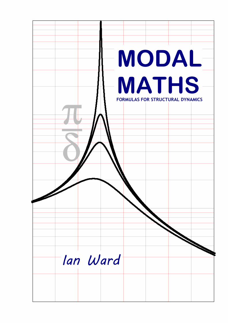
π

δ

MODAL

MATHS FORMULAS FOR STRUCTURAL DYNAMICS

Ian Ward

Time

CK

M x

< critical damping

critically damped

> critical damping

Time

Displace

ment

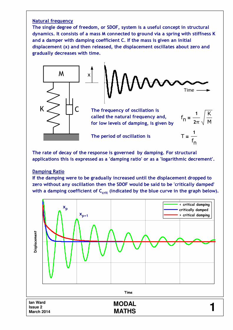
Natural frequency

The single degree of freedom, or SDOF, system is a useful concept in structural

dynamics. It consists of a mass M connected to ground via a spring with stiffness K

and a damper with damping coefficient C. If the mass is given an initial

displacement (x) and then released, the displacement oscillates about zero and

gradually decreases with time.

The frequency of oscillation is

called the natural frequency and,

for low levels of damping, is given byfn

1

2π

K

M=

The period of oscillation is T1

fn

=

The rate of decay of the response is governed by damping. For structural

applications this is expressed as a 'damping ratio' or as a 'logarithmic decrement'.

Damping Ratio

If the damping were to be gradually increased until the displacement dropped to

zero without any oscillation then the SDOF would be said to be 'critically damped'

with a damping coefficient of Ccrit (indicated by the blue curve in the graph below).

xp

xp+1

Ian Ward Issue 2 March 2014

MODALMATHS 1

Any further increase in the damping would give rise to a slower decay to zero

(the red curve in the graph). In practice, structural damping is only a fraction of

the critical value and the decay of vibration is more closely represented by the

green curve in the graph. The amount of damping can be defined in terms of a

critical damping ratio:

damping ratio ξC

Ccrit

=

The relationship between the damping ratio and the damping coefficient is

C 2ξMω= 2ξ MK=

with the circular frequency ω given by ω 2π f=

Logarithmic Decrement

An alternative way of describing the structural damping is to consider the height

of successive peaks in the vibration decay (denoted as xp and xp+1 in the graph on

the previous page). The natural logarithm of this ratio is the logarithmic

decrement δ (or 'log. dec.'):

logarithmic decrement δ lnxp

xp 1+

= i.e.xp

xp 1+

eδ

=

Or, if the decay over a number of cycles N is considered then

logarithmic decrement δ1

Nln

xp

xp N+

= i.e.xp

xp N+

eNδ

=

The relationship between the logarithmic decrement and the damping ratio is

δ 2πξ=

As a rough guide, a logarithmic decrement of 0.1 means that the peak amplitude

falls by approximately 10% in each successive cycle.

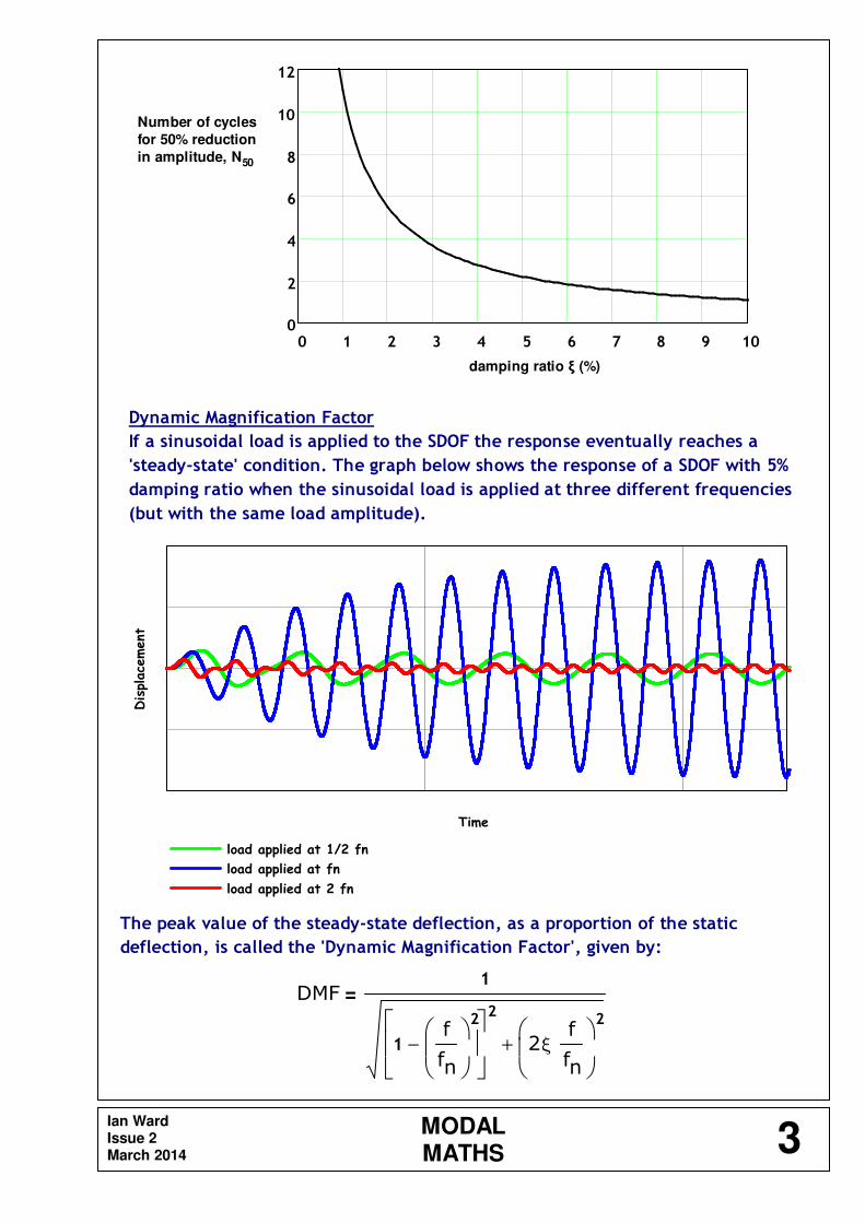
Another way of visualizing the vibration decay associated with a particular

damping value is by showing that the number of cycles required to cause the peak

amplitude to decay by, say, 50% is:

(this relationship is shown

in the graph overleaf)N50

ln1

0.5

δ=

ln 2( )

δ=

ln 2( )

2πξ=


MODALMATHS 2

0 1 2 3 4 5 6 7 8 9 100

2

4

6

8

10

12

load applied at 1/2 fn

load applied at fn

load applied at 2 fn

Time

Displace

ment

Number of cycles

for 50% reduction

in amplitude, N50

damping ratio ξ (%)

Dynamic Magnification Factor

If a sinusoidal load is applied to the SDOF the response eventually reaches a

'steady-state' condition. The graph below shows the response of a SDOF with 5%

damping ratio when the sinusoidal load is applied at three different frequencies

(but with the same load amplitude).

The peak value of the steady-state deflection, as a proportion of the static

deflection, is called the 'Dynamic Magnification Factor', given by:

DMF1

1f

fn

2

−

2

2ξf

fn

2

+

=


MODALMATHS 3

0 0.2 0.4 0.6 0.8 1 1.2 1.4 1.6 1.8 20.1

1

10

100damping ratio = 0.5%

damping ratio = 2%

damping ratio = 5%

damping ratio = 10%

damping ratio = 20%

22

DMF versus frequency ratio for different levels of damping

DMF

Note that, for high levels of damping,

the maximum response (resonance)

occurs when the forcing frequency is

slightly lower than the natural

frequency. For low damping levels,

when the forcing frequency increases

above the natural frequency the

response decreases back down to the

static value when f 2 fn=

frequency ratio f/fn


MODALMATHS 4

Frequency

DMF

The maximum DMF occurs when the forcing frequency is

fmax fn 1 2ξ2

−=

The value of the maximum DMF is

DMFmax1

2ξ=

π

δ=

From this it follows that the displacement at resonance is

xres1

2ξ

F

K=

π

δ

F

K=

and the acceleration at resonance is

ares1

2ξ

F

M=

π

δ

F

M=

The DMF curve also supplies a means for determining the damping ratio:

where >f is the width of the DMF curve at 1

2

times the resonant amplitude at frequency fmax.

ξ∆∆∆∆f

2fmax

=

This is referred to as the half-power bandwidth method for determining the

damping, and is shown graphically in the figure below.

DMFmax

>f DMFmax

2

fmax


MODALMATHS 5

Build-up of Resonant Response

The response after a number of cycles, N, as a proportion of the final resonant

response is given by:

x

xres1 e

2− πξN−( )=

This expression is illustrated in the figure below for a number of different damping

ratios.

0 10 20 30 40 50 60 70 80 90 1000

0.25

0.5

0.75

1

damping ratio = 5%

damping ratio = 2%

damping ratio = 1%

damping ratio = 0.5%

0.96

x/xres

Number of cycles to achieve resonance, N

An approximate relationship for the number of cycles required to reach the

maximum resonant response (strictly speaking, 96% of it) is:

Npeak1

2ξ=

π

δ=

The figure shows that roughly the same number of cycles again are required for

the response to build up from 96% to 100% of the maximum resonant response.


MODALMATHS 6

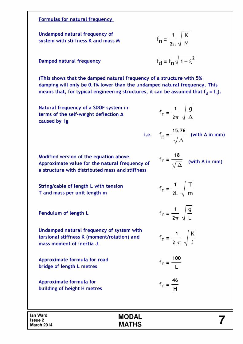
Formulas for natural frequency

Undamped natural frequency of

system with stiffness K and mass M fn1

2π

K

M=

Damped natural frequency fd fn 1 ξ2

−=

(This shows that the damped natural frequency of a structure with 5%

damping will only be 0.1% lower than the undamped natural frequency. This

means that, for typical engineering structures, it can be assumed that fd = fn).

Natural frequency of a SDOF system in

terms of the self-weight deflection >

caused by 1g

fn1

2π

g

∆=

i.e. fn15.76

∆= (with > in mm)

Modified version of the equation above.

Approximate value for the natural frequency of

a structure with distributed mass and stiffness

fn18

∆= (with > in mm)

String/cable of length L with tension

T and mass per unit length mfn

1

2L

T

m=

Pendulum of length L fn1

2π

g

L=

Undamped natural frequency of system with

torsional stiffness K (moment/rotation) and

mass moment of inertia J.fn

1

2 π

K

J=

Approximate formula for road

bridge of length L metres fn

100

L=

Approximate formula for

building of height H metres fn

46

H=


MODALMATHS 7

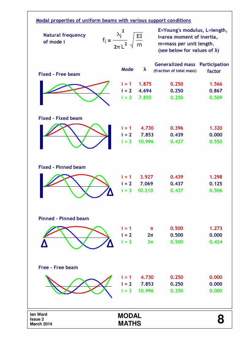
Natural frequency

of mode i fi

λi2

2πL2

EI

m=

Generalized mass

(fraction of total mass)

Participation

factorMode λ Fixed - Free beam

i = 1

i = 2

i = 3

1.875

4.694

7.855

0.250

0.250

0.250

1.566

0.867

0.509

Fixed - Fixed beam

i = 1

i = 2

i = 3

4.730

7.853

10.996

0.396

0.439

0.437

1.320

0.000

0.550

Fixed - Pinned beam

Modal properties of uniform beams with various support conditions

i = 1

i = 2

i = 3

3.927

7.069

10.210

0.439

0.437

0.437

1.298

0.125

0.506>

Pinned - Pinned beam

E=Young's modulus, L=length,

I=area moment of inertia,

m=mass per unit length.

(see below for values of λ)

i = 1

i = 2

i = 3

π

2π

3π

0.500

0.500

0.500

1.273

0.000

0.424> >

Free - Free beam

i = 1

i = 2

i = 3

4.730

7.853

10.996

0.250

0.250

0.250

0.000

0.000

0.000


MODALMATHS 8

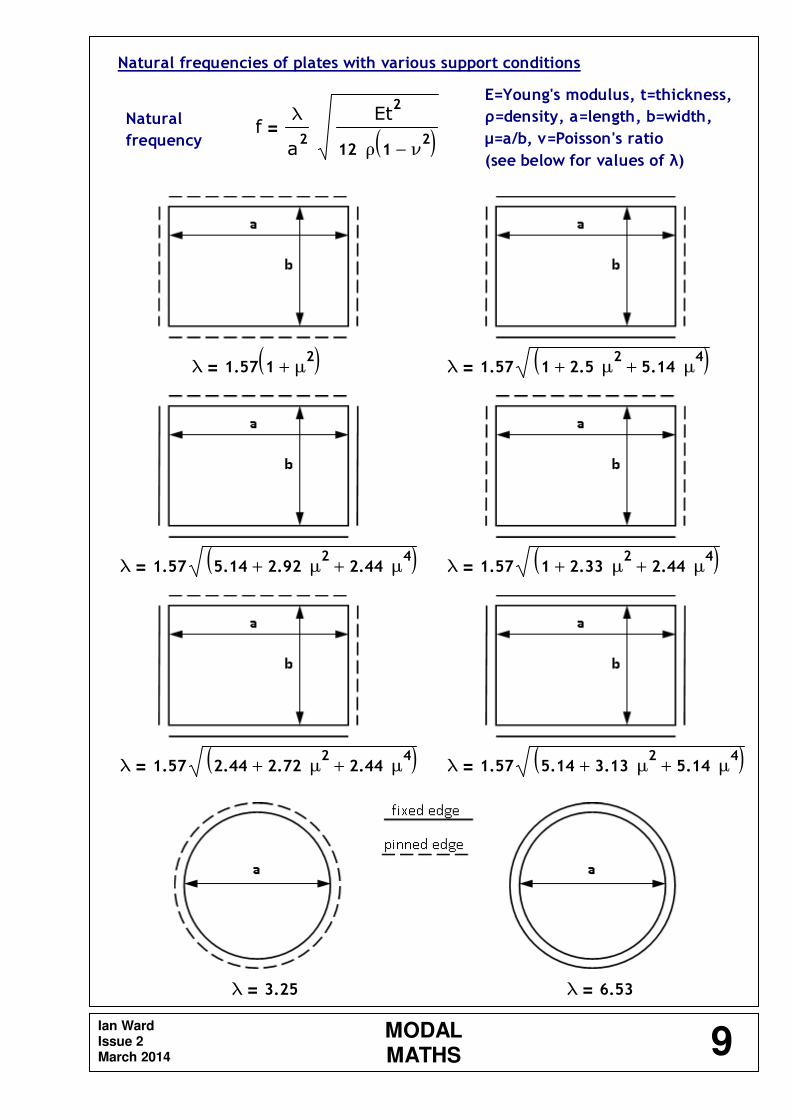
Natural frequencies of plates with various support conditions

E=Young's modulus, t=thickness,

ρ=density, a=length, b=width,

µ=a/b, ν=Poisson's ratio

(see below for values of λ)

Natural

frequency f

λ

a2

Et2

12 ρ 1 ν2

−( )=

λ 1.57 1 μ2

+( )= λ 1.57 1 2.5 μ2

+ 5.14 μ4

+( )=

λ 1.57 5.14 2.92 μ2

+ 2.44 μ4

+( )= λ 1.57 1 2.33 μ2

+ 2.44 μ4

+( )=

λ 1.57 2.44 2.72 μ2

+ 2.44 μ4

+( )= λ 1.57 5.14 3.13 μ2

+ 5.14 μ4

+( )=

λ 3.25= λ 6.53=


MODALMATHS 9

0 0.5 1 1.5 2 2.5 3 3.5 4 4.5 50

0.2

0.4

0.6

0.8

1

1.2

1.4

1.6

1.8

2

2.2

Maximum Response of an Undamped SDOF Elastic System

Subject to Various Load Pulses

DLFmax

K period T

force

M

time

force

td

time

force

td

time

force

td

time

force

td

time

force

td

td/T

In the derivation of these charts no damping has been included because it has no

significant effect. The maximum DLF usually corresponds to the first peak of

response, and the amount of damping normally encountered in structures is not

sufficient to sigificantly decrease this value.


MODALMATHS 10

ξa(%)

Tuned Mass Dampers

The TMD design chart below gives the

additional overall damping ratio (ξa)

provided by a TMD when attached to a

structure with inherent damping ξs.

The chart is based on a TMD with ξd=15%

and a structure with ξs in the range

0.5% - 2.5%. It also assumes that the TMD

is located at the position of maximum

response of the mode being damped.

The overall damping becomes ξs + ξa.

Tuned

Mass

Damper

Structure

modal

mass

ratio

Md/Ms

(%)

frequency ratio fd/fs (%)


MODALMATHS 11

me0

L

xm x( ) ϕ x( )2⌠

⌡

d

0

L

xϕ x( )2⌠

⌡

d

=

Tuned Mass Dampers

If the TMD can be tuned then the TMD chart

shows that the additional damping is roughly

ξa

Md

Ms

=

Maximum deflection of

TMD relative to structurexreld

1

2ξd

=π

δd

=

Optimum TMD frequency fd

fs

1 μ+= with μ

Md

Ms

=

Optimum TMD damping ratio ξd3 μ

8 1 μ+( )3

=

Wind-induced vortex shedding

fn=natural frequency,

D=across-wind dimension,

St=Strouhal number.

Critical wind speed

for vortex sheddingvcrit

fn D

St=

For a circular cylinder St is approximately 0.2 and therefore vcrit 5 fn D=

The susceptibility of vortex-induced vibrations depends on the structural damping

and the ratio of the structural mass to the fluid mass. This is expressed by the

Scruton number (Sc), also known as the 'mass-damping parameter'.

(equivalent mass

per unit length)Sc2 me δs

ρair D2

= with

Wind-induced galloping

dCy/dα is the rate of change

of the lateral force coefficient

with angle of attack

Critical wind speed

for gallopingvcrit

2 Sc fn D

dCy

dα

=

A section

is susceptible

to galloping if

dCy

dα0> note that

dCy

dα

dCL

dαCD+

−=

with CL=lift coefficient, CD=drag coefficient


MODALMATHS 12

M

S a

fn

Seismic Response Spectrum Analysis

Relationship between SDOF response and structure response for each mode.

Single Degree of Freedom

fn

frequency

Structure with distributed mass/stiffness

Generalized mass

(modal mass)MG

0

L

xϕ x( )2ml x( )⋅

⌠⌡

d=

Participation

factorΓ

0

L

xϕ x( ) ml x( )⋅⌠⌡

d

0

L

xϕ x( )2ml x( )⋅

⌠⌡

d

=natural

frequency fn

mode shape

ϕϕϕϕ(x)L

Maximum

acceleration

at point i

ai Sa Γ⋅ ϕ xi( )⋅=

mass per

unit length

ml(x)

Effective mass ME0

L

xϕ x( ) ml x( )⋅⌠⌡

d

2

0

L

xϕ x( )2ml x( )⋅

⌠⌡

d

=

Base shear SFbase Sa ME⋅=

The maximum response from each of the modes can be combined using the 'Square

Root Sum of Squares' (SRSS) or 'Complete Quadratic Combination' (CQC) method.

spectral acceleration

Ian Ward Issue 2March 2014

MODALMATHS 13

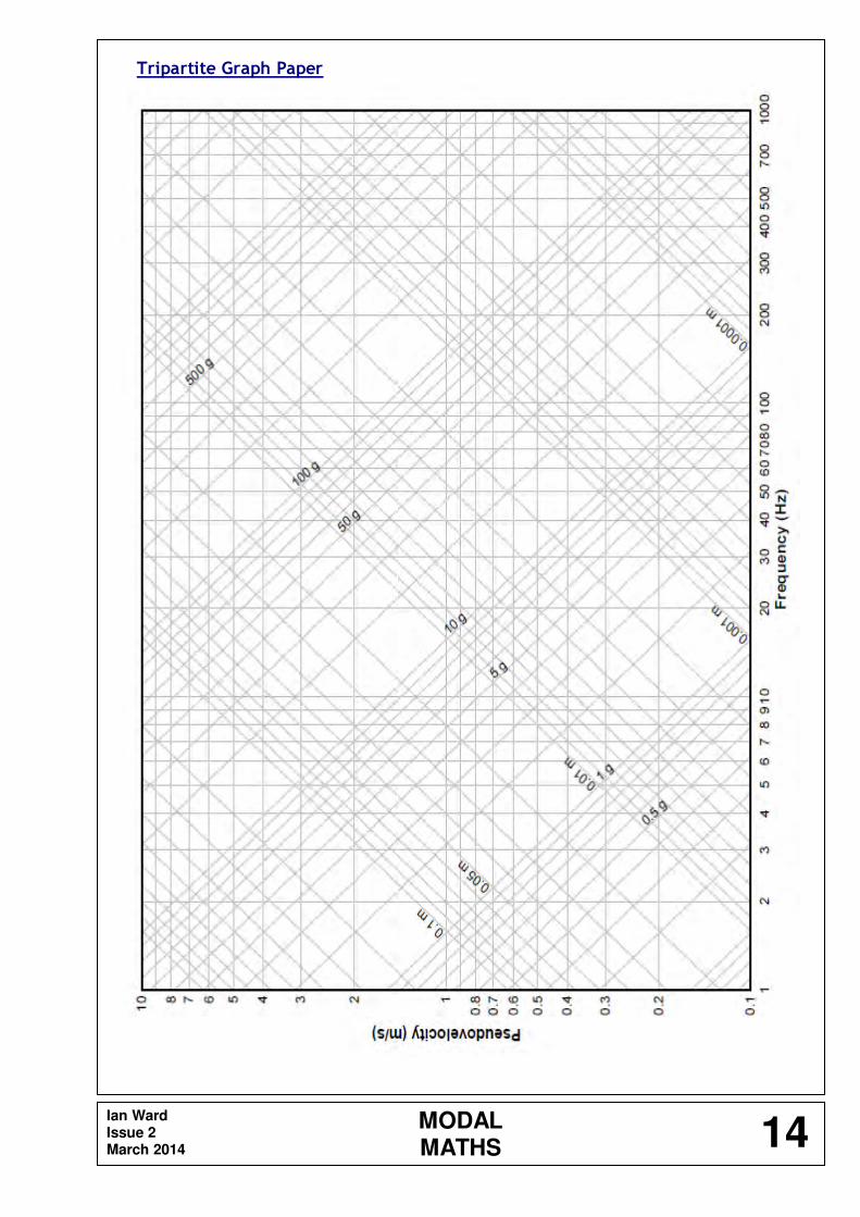
Tripartite Graph Paper


MODALMATHS 14

References

Bachmann H., Ammann W., 'Vibrations in Structures Induced by Man and•

Machines'. IABSE. 1987.

Barltrop N.D.P., Adams A.J., ‘Dynamics of Fixed Marine Structures’. 3rd•

Edition. MTD. 1991.

Biggs J.M., ‘Introduction to Structural Dynamics’. McGraw-Hill. 1964.•

Blevins R.D. ‘Formulas for Natural Frequency and Mode Shape’. Van Nostrand•

Reinhold. 1979.

Blevins R.D., ‘Flow-Induced Vibration’. Second Edition. Krieger. 2001.•

Chopra A.K., ‘Dynamics of Structures – A Primer’. Earthquake Engineering•

Research Institute. 1981.

Chopra A.K., ‘Dynamics of Structures – Theory and Applications to Earthquake•

Engineering’. Prentice Hall. 1995.

Clough R.W., Penzien J., ‘Dynamics of Structures’. Computers and Structures•

Inc. Second edition. 2003.

Coates R.C., Coutie M.G., Kong F.K., ‘Structural Analysis’. Chapman & Hall.•

1997.

Craig R.R., ‘Structural Dynamics – An Introduction to Computer Methods’. John•

Wiley. 1981.

Den Hartog J.P., ‘Mechanical Vibrations’. McGraw-Hill. 1956.•

DynamAssist structural dynamics toolbox. www.DynamAssist.com.•

Gupta A.K. ‘Response Spectrum Method in Seismic Analysis and Design of•

Structures’. Blackwell Scientific Publications. 1990.

Irvine H.M., ‘Structural Dynamics for the Practising Engineer’. Allen and•

Unwin. 1986.

Karnovsky I.A., Lebed O.I., ‘Formulas for Structural Dynamics: Tables, Graphs•

and Solutions’. McGraw-Hill. 2001.

Maguire J.R., Wyatt T.R., 'Dynamics An Introduction for Civil and Structural•

Engineers'. ICE Design and Practice Guide. Thomas Telford. 1999.

Mead D.J., 'Passive Vibration Control'. John Wiley and Sons. 1998.•

Neumark N.M., Rosenbleuth E.,’Fundamentals of Earthquake Engineering’.•

Prentice-Hall. 1971.

Norris C.H. et al ‘Structural Design for Dynamic Loads’. McGraw-Hill. 1959.•

Scruton C., 'An Introduction to Wind Effects on Structures'. Engineering Design•

Guide 40. Oxford University Press.

Simiu E., Scanlan R.H., ‘Wind Effects on Structures – An Introduction to Wind•

Engineering’. John Wiley and Sons. 1986

Young W.C. 'Roark's Formulas for Stress and Strain'. McGraw-Hill. Sixth•

Edition. 1989.


MODALMATHS 15

Terminology

δ logarithmic decrement

Ff frequency interval

ξ damping ratio

ω circular frequency (2πf)

ν Poisson's ratio

Γ participation factor

ϕϕϕϕ mode shape

µ aspect ratio, mass ratio

ρ density

F self-weight deflection

a acceleration

C damping coefficient

Ccrit critical damping coefficient

CD drag coefficient

CL lift coefficient

Cy lateral force coefficient

D across-wind dimension

DMF dynamic magnification factor

E Young's modulus

f frequency

fd damped natural frequency

fi natural frequency of mode i

fn undamped natural frequency

g acceleration due to gravity

h plate thickness

H height

J mass moment of inertia

K stiffness

L length

ml mass per unit length

M mass

ME effective mass

MG generalized mass

N number of cycles

SDOF single degree of freedom

Sc Scruton number

St Strouhal number

t time, thickness

T period, tension

x displacement


MODALMATHS 16

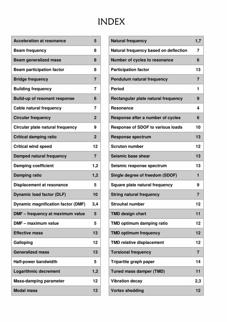
INDEX

Acceleration at resonance 5 Natural frequency 1,7

Beam frequency 8 Natural frequency based on deflection 7

Beam generalized mass 8 Number of cycles to resonance 6

Beam participation factor 8 Participation factor 13

Bridge frequency 7 Pendulum natural frequency 7

Building frequency 7 Period 1

Build-up of resonant response 6 Rectangular plate natural frequency 9

Cable natural frequency 7 Resonance 4

Circular frequency 2 Response after a number of cycles 6

Circular plate natural frequency 9 Response of SDOF to various loads 10

Critical damping ratio 2 Response spectrum 13

Critical wind speed 12 Scruton number 12

Damped natural frequency 7 Seismic base shear 13

Damping coefficient 1,2 Seismic response spectrum 13

Damping ratio 1,2 Single degree of freedom (SDOF) 1

Displacement at resonance 5 Square plate natural frequency 9

Dynamic load factor (DLF) 10 String natural frequency 7

Dynamic magnification factor (DMF) 3,4 Strouhal number 12

DMF – frequency at maximum value 5 TMD design chart 11

DMF – maximum value 5 TMD optimum damping ratio 12

Effective mass 13 TMD optimum frequency 12

Galloping 12 TMD relative displacement 12

Generalized mass 13 Torsional frequency 7

Half-power bandwidth 5 Tripartite graph paper 14

Logarithmic decrement 1,2 Tuned mass damper (TMD) 11

Mass-damping parameter 12 Vibration decay 2,3

Modal mass 13 Vortex shedding 12

FORMULAS FOR STRUCTURAL DYNAMICS δ−−−− Maths Issue 2.pdf · The single degree of freedom,...

Documents

Transcript of FORMULAS FOR STRUCTURAL DYNAMICS δ−−−− Maths Issue 2.pdf · The single degree of freedom,...