Computational Fluid Dynamics - Uni Ulm Aktuelles ... 1Introduction j Computational Fluid Dynamics j...
144
Seite 1 Introduction | Computational Fluid Dynamics | 03.07.2017 Computational Fluid Dynamics Theory, Numerics, Modelling Lucas Engelhardt Computational Biomechanics Summer Term 2017
Transcript of Computational Fluid Dynamics - Uni Ulm Aktuelles ... 1Introduction j Computational Fluid Dynamics j...
Seite 1 Introduction | Computational Fluid Dynamics | 03.07.2017
Computational Fluid DynamicsTheory, Numerics, Modelling
Lucas Engelhardt
Computational Biomechanics
Summer Term 2017

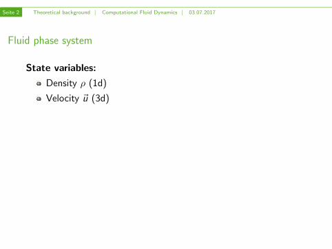
Seite 2 Theoretical background | Computational Fluid Dynamics | 03.07.2017
Fluid phase system
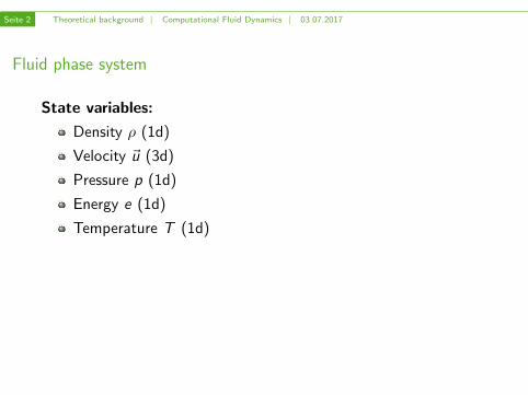
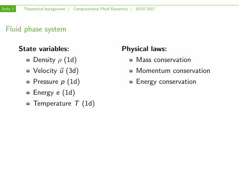
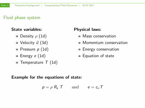
State variables:
Density ρ (1d)
Velocity ~u (3d)
Pressure p (1d)
Energy e (1d)
Temperature T (1d)
Physical laws:
Mass conservation
Momentum conservation
Energy conservation
Equation of state
Example for the equations of state:
p = ρ Rs T and e = cνT
Seite 2 Theoretical background | Computational Fluid Dynamics | 03.07.2017
Fluid phase system
State variables:
Density ρ (1d)
Velocity ~u (3d)
Pressure p (1d)
Energy e (1d)
Temperature T (1d)
Physical laws:
Mass conservation
Momentum conservation
Energy conservation
Equation of state
Example for the equations of state:
p = ρ Rs T and e = cνT
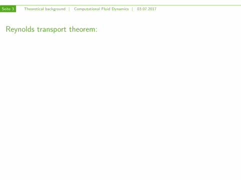
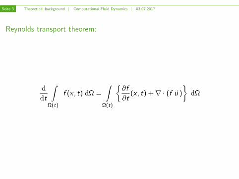
Seite 3 Theoretical background | Computational Fluid Dynamics | 03.07.2017
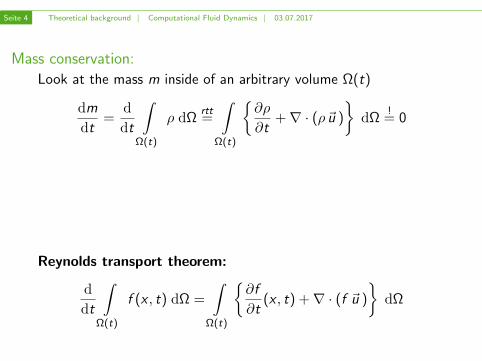
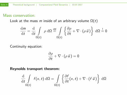
Reynolds transport theorem:
d
dt
∫Ω(t)
f (x , t) dΩ =
∫Ω(t)
∂f
∂t(x , t) +∇ · (f ~u )
dΩ
Seite 3 Theoretical background | Computational Fluid Dynamics | 03.07.2017
Reynolds transport theorem:
d
dt
∫Ω(t)
f (x , t) dΩ =
∫Ω(t)
∂f
∂t(x , t) +∇ · (f ~u )
dΩ
Seite 4 Theoretical background | Computational Fluid Dynamics | 03.07.2017
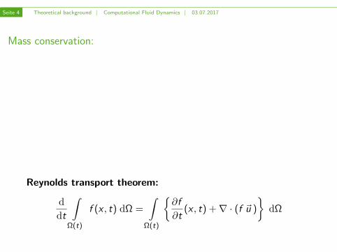
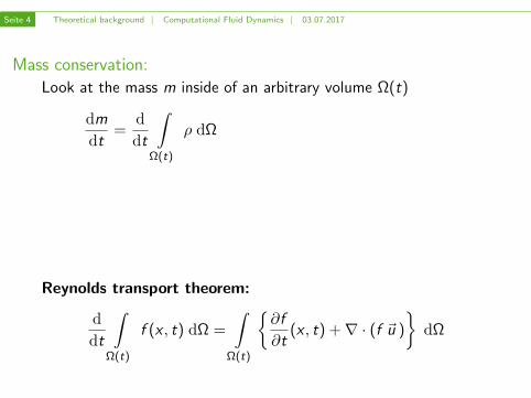
Mass conservation:
Look at the mass m inside of an arbitrary volume Ω(t)
dm
dt=
d
dt
∫Ω(t)
ρ dΩ
rtt=
∫Ω(t)
∂ρ
∂t+∇ · (ρ~u )
dΩ
!= 0
Continuity equation:
∂ρ
∂t+∇ · (ρ~u ) = 0
Reynolds transport theorem:
d
dt
∫Ω(t)
f (x , t) dΩ =
∫Ω(t)
∂f
∂t(x , t) +∇ · (f ~u )
dΩ
Seite 4 Theoretical background | Computational Fluid Dynamics | 03.07.2017
Mass conservation:
Look at the mass m inside of an arbitrary volume Ω(t)
dm
dt=
d
dt
∫Ω(t)
ρ dΩ
rtt=
∫Ω(t)
∂ρ
∂t+∇ · (ρ~u )
dΩ
!= 0
Continuity equation:
∂ρ
∂t+∇ · (ρ~u ) = 0
Reynolds transport theorem:
d
dt
∫Ω(t)
f (x , t) dΩ =
∫Ω(t)
∂f
∂t(x , t) +∇ · (f ~u )
dΩ

Seite 4 Theoretical background | Computational Fluid Dynamics | 03.07.2017
Mass conservation:
Look at the mass m inside of an arbitrary volume Ω(t)
dm
dt=
d
dt
∫Ω(t)
ρ dΩrtt=
∫Ω(t)
∂ρ
∂t+∇ · (ρ~u )
dΩ
!= 0
Continuity equation:
∂ρ
∂t+∇ · (ρ~u ) = 0
Reynolds transport theorem:
d
dt
∫Ω(t)
f (x , t) dΩ =
∫Ω(t)
∂f
∂t(x , t) +∇ · (f ~u )
dΩ
Seite 5 Theoretical background | Computational Fluid Dynamics | 03.07.2017
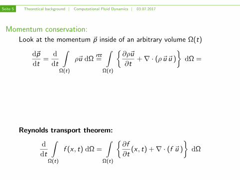
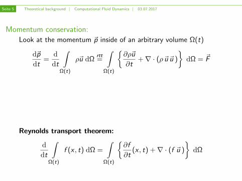
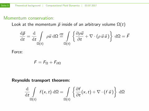
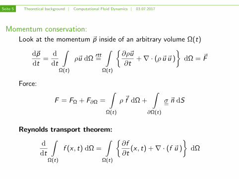
Momentum conservation:
Look at the momentum ~p inside of an arbitrary volume Ω(t)
d~p
dt=
d
dt
∫Ω(t)
ρ~u dΩrtt=
∫Ω(t)
∂ρ~u
∂t+∇ · (ρ~u ~u )
dΩ =
~F
Force:
F = FΩ + F∂Ω
=
∫Ω(t)
ρ ~f dΩ +
∫∂Ω(t)
σ ~n dS
Reynolds transport theorem:
d
dt
∫Ω(t)
f (x , t) dΩ =
∫Ω(t)
∂f
∂t(x , t) +∇ · (f ~u )
dΩ
Seite 5 Theoretical background | Computational Fluid Dynamics | 03.07.2017
Momentum conservation:
Look at the momentum ~p inside of an arbitrary volume Ω(t)
d~p
dt=
d
dt
∫Ω(t)
ρ~u dΩrtt=
∫Ω(t)
∂ρ~u
∂t+∇ · (ρ~u ~u )
dΩ = ~F
Force:
F = FΩ + F∂Ω =
∫Ω(t)
ρ ~f dΩ +
∫∂Ω(t)
σ ~n dS
Reynolds transport theorem:
d
dt
∫Ω(t)
f (x , t) dΩ =
∫Ω(t)
∂f
∂t(x , t) +∇ · (f ~u )
dΩ
Seite 6 Theoretical background | Computational Fluid Dynamics | 03.07.2017
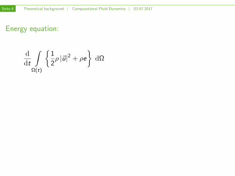
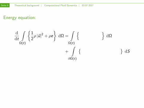
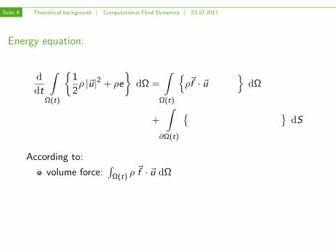
Energy equation:
d
dt
∫Ω(t)
1
2ρ |~u|2 + ρe
dΩ
=
∫Ω(t)
ρ~f · ~u + ρ Q
dΩ
+
∫∂Ω(t)
(σ ~n
)· ~u + κ ∇T · ~n
dS
According to:
volume force:∫
Ω(t) ρ~f · ~u dΩ
energy source:∫
Ω(t) ρ Q dΩ
surface force:∫∂Ω(t)
(σ ~n
)· ~u dS
heat flux:∫∂Ω(t) κ ∇T · ~n dS
Seite 6 Theoretical background | Computational Fluid Dynamics | 03.07.2017
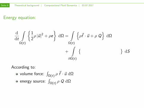
Energy equation:
d
dt
∫Ω(t)
1
2ρ |~u|2 + ρe
dΩ =
∫Ω(t)
ρ~f · ~u + ρ Q
dΩ
+
∫∂Ω(t)
(σ ~n
)· ~u + κ ∇T · ~n
dS
According to:
volume force:∫
Ω(t) ρ~f · ~u dΩ
energy source:∫
Ω(t) ρ Q dΩ
surface force:∫∂Ω(t)
(σ ~n
)· ~u dS
heat flux:∫∂Ω(t) κ ∇T · ~n dS
Seite 6 Theoretical background | Computational Fluid Dynamics | 03.07.2017
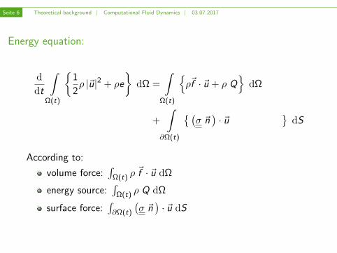
Energy equation:
d
dt
∫Ω(t)
1
2ρ |~u|2 + ρe
dΩ =
∫Ω(t)
ρ~f · ~u
+ ρ Q
dΩ
+
∫∂Ω(t)
(σ ~n
)· ~u + κ ∇T · ~n
dS
According to:
volume force:∫
Ω(t) ρ~f · ~u dΩ
energy source:∫
Ω(t) ρ Q dΩ
surface force:∫∂Ω(t)
(σ ~n
)· ~u dS
heat flux:∫∂Ω(t) κ ∇T · ~n dS
Seite 6 Theoretical background | Computational Fluid Dynamics | 03.07.2017
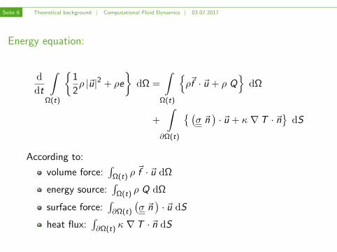
Energy equation:
d
dt
∫Ω(t)
1
2ρ |~u|2 + ρe
dΩ =
∫Ω(t)
ρ~f · ~u + ρ Q
dΩ
+
∫∂Ω(t)
(σ ~n
)· ~u + κ ∇T · ~n
dS
According to:
volume force:∫
Ω(t) ρ~f · ~u dΩ
energy source:∫
Ω(t) ρ Q dΩ
surface force:∫∂Ω(t)
(σ ~n
)· ~u dS
heat flux:∫∂Ω(t) κ ∇T · ~n dS
Seite 6 Theoretical background | Computational Fluid Dynamics | 03.07.2017
Energy equation:
d
dt
∫Ω(t)
1
2ρ |~u|2 + ρe
dΩ =
∫Ω(t)
ρ~f · ~u + ρ Q
dΩ
+
∫∂Ω(t)
(σ ~n
)· ~u
+ κ ∇T · ~n
dS
According to:
volume force:∫
Ω(t) ρ~f · ~u dΩ
energy source:∫
Ω(t) ρ Q dΩ
surface force:∫∂Ω(t)
(σ ~n
)· ~u dS
heat flux:∫∂Ω(t) κ ∇T · ~n dS
Seite 6 Theoretical background | Computational Fluid Dynamics | 03.07.2017
Energy equation:
d
dt
∫Ω(t)
1
2ρ |~u|2 + ρe
dΩ =
∫Ω(t)
ρ~f · ~u + ρ Q
dΩ
+
∫∂Ω(t)
(σ ~n
)· ~u + κ ∇T · ~n
dS
According to:
volume force:∫
Ω(t) ρ~f · ~u dΩ
energy source:∫
Ω(t) ρ Q dΩ
surface force:∫∂Ω(t)
(σ ~n
)· ~u dS
heat flux:∫∂Ω(t) κ ∇T · ~n dS
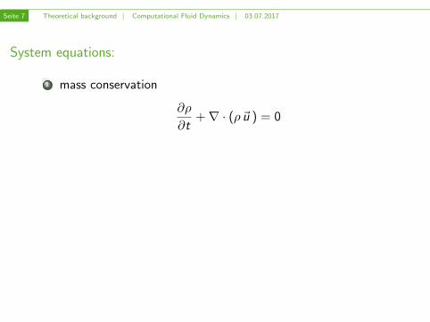
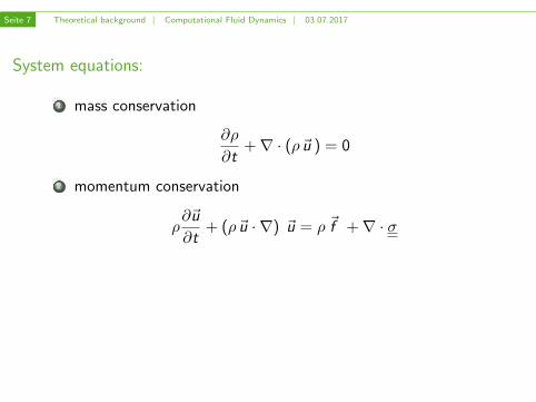
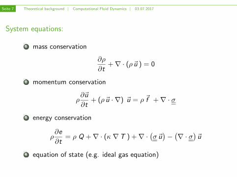
Seite 7 Theoretical background | Computational Fluid Dynamics | 03.07.2017
System equations:
1 mass conservation
∂ρ
∂t+∇ · (ρ~u ) = 0
2 momentum conservation
ρ∂~u
∂t+ (ρ~u · ∇) ~u = ρ ~f +∇ · σ
3 energy conservation
ρ∂e
∂t= ρ Q +∇ · (κ ∇T ) +∇ ·
(σ~u)−(∇ · σ
)~u
4 equation of state (e.g. ideal gas equation)

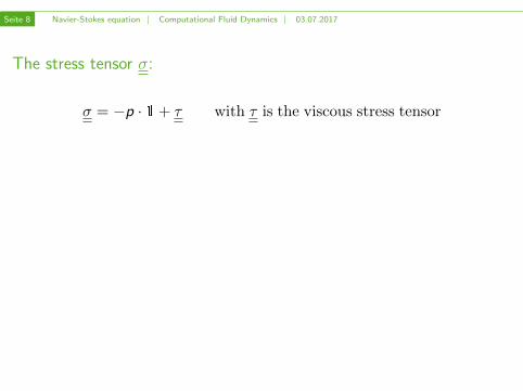
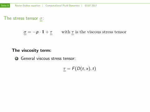
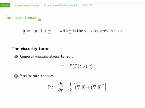
Seite 8 Navier-Stokes equation | Computational Fluid Dynamics | 03.07.2017
The stress tensor σ:
σ = −p · 1 + τ with τ is the viscous stress tensor
The viscosity term:
1 General viscous stress tensor:
τ = F (D(t, x), t)
2 Strain rate tensor:
D :=∂ε
∂t=
1
2
[(∇ ~u) + (∇ ~u)T
]
Seite 8 Navier-Stokes equation | Computational Fluid Dynamics | 03.07.2017
The stress tensor σ:
σ = −p · 1 + τ with τ is the viscous stress tensor
The viscosity term:
1 General viscous stress tensor:
τ = F (D(t, x), t)
2 Strain rate tensor:
D :=∂ε
∂t=
1
2
[(∇ ~u) + (∇ ~u)T
]
Seite 8 Navier-Stokes equation | Computational Fluid Dynamics | 03.07.2017
The stress tensor σ:
σ = −p · 1 + τ with τ is the viscous stress tensor
The viscosity term:
1 General viscous stress tensor:
τ = F (D(t, x), t)
2 Strain rate tensor:
D :=∂ε
∂t=
1
2
[(∇ ~u) + (∇ ~u)T
]
Seite 8 Navier-Stokes equation | Computational Fluid Dynamics | 03.07.2017
The stress tensor σ:
σ = −p · 1 + τ with τ is the viscous stress tensor
The viscosity term:
1 General viscous stress tensor:
τ = F (D(t, x), t)
2 Strain rate tensor:
D :=∂ε
∂t=
1
2
[(∇ ~u) + (∇ ~u)T
]
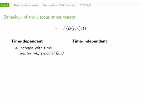
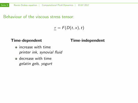
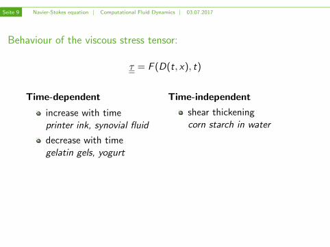
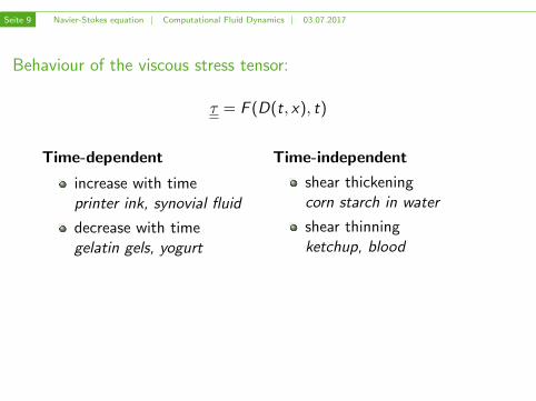
Seite 9 Navier-Stokes equation | Computational Fluid Dynamics | 03.07.2017
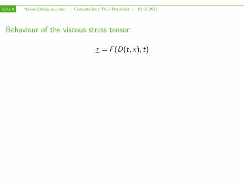
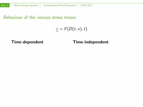
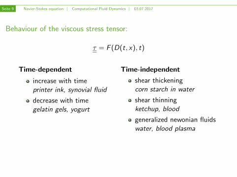
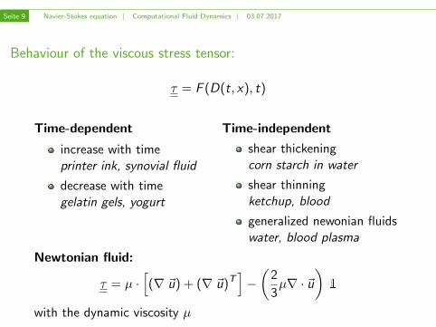
Behaviour of the viscous stress tensor:
τ = F (D(t, x), t)
Time-dependent Time-independent
increase with timeprinter ink, synovial fluid
decrease with timegelatin gels, yogurt
shear thickeningcorn starch in water
shear thinningketchup, blood
generalized newonian fluidswater, blood plasma
Newtonian fluid:
τ = µ ·[(∇ ~u) + (∇ ~u)T
]−(
2
3µ∇ · ~u
)1
with the dynamic viscosity µ
Seite 9 Navier-Stokes equation | Computational Fluid Dynamics | 03.07.2017
Behaviour of the viscous stress tensor:
τ = F (D(t, x), t)
Time-dependent Time-independent
increase with timeprinter ink, synovial fluid
decrease with timegelatin gels, yogurt
shear thickeningcorn starch in water
shear thinningketchup, blood
generalized newonian fluidswater, blood plasma
Newtonian fluid:
τ = µ ·[(∇ ~u) + (∇ ~u)T
]−(
2
3µ∇ · ~u
)1
with the dynamic viscosity µ

Seite 10 Navier-Stokes equation | Computational Fluid Dynamics | 03.07.2017
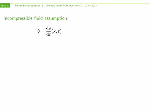
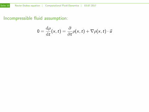
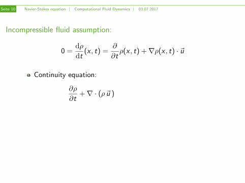
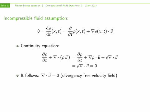
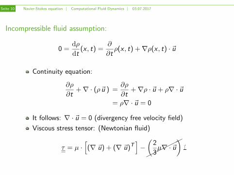
Incompressible fluid assumption:
0 =dρ
dt(x , t)
=∂
∂tρ(x , t) +∇ρ(x , t) · ~u
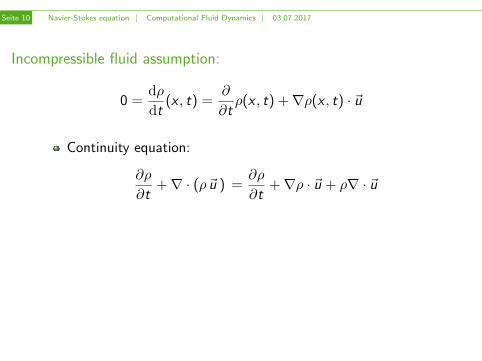
Continuity equation:
∂ρ
∂t+∇ · (ρ~u )
=∂ρ
∂t+∇ρ · ~u + ρ∇ · ~u
= ρ∇ · ~u = 0
It follows: ∇ · ~u = 0 (divergency free velocity field)
Viscous stress tensor: (Newtonian fluid)
τ = µ ·[(∇ ~u) + (∇ ~u)T
]−
(
2
3µ∇ · ~u
)1
Seite 10 Navier-Stokes equation | Computational Fluid Dynamics | 03.07.2017
Incompressible fluid assumption:
0 =dρ
dt(x , t)
=∂
∂tρ(x , t) +∇ρ(x , t) · ~u
Continuity equation:
∂ρ
∂t+∇ · (ρ~u )
=∂ρ
∂t+∇ρ · ~u + ρ∇ · ~u
= ρ∇ · ~u = 0
It follows: ∇ · ~u = 0 (divergency free velocity field)
Viscous stress tensor: (Newtonian fluid)
τ = µ ·[(∇ ~u) + (∇ ~u)T
]−
(
2
3µ∇ · ~u
)1
Seite 10 Navier-Stokes equation | Computational Fluid Dynamics | 03.07.2017
Incompressible fluid assumption:
0 =dρ
dt(x , t) =
∂
∂tρ(x , t) +∇ρ(x , t) · ~u
Continuity equation:
∂ρ
∂t+∇ · (ρ~u ) =
∂ρ
∂t+∇ρ · ~u + ρ∇ · ~u
= ρ∇ · ~u = 0
It follows: ∇ · ~u = 0 (divergency free velocity field)
Viscous stress tensor: (Newtonian fluid)
τ = µ ·[(∇ ~u) + (∇ ~u)T
]−
(
2
3µ∇ · ~u
)1
Seite 11 Navier-Stokes equation | Computational Fluid Dynamics | 03.07.2017
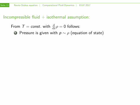
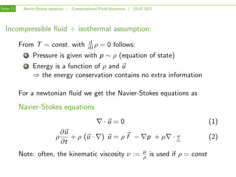
Incompressible fluid + isothermal assumption:
From T = const. with ddt ρ = 0 follows:
1 Pressure is given with p ∼ ρ (equation of state)
2 Energy is a function of ρ and ~u⇒ the energy conservation contains no extra information
For a newtonian fluid we get the Navier-Stokes equations as
Navier-Stokes equations
∇ · ~u = 0 (1)
ρ∂~u
∂t+ ρ (~u · ∇) ~u = ρ ~f −∇p + µ∇ · τ (2)
Note: often, the kinematic viscosity ν := µρ is used if ρ = const
Seite 11 Navier-Stokes equation | Computational Fluid Dynamics | 03.07.2017
Incompressible fluid + isothermal assumption:
From T = const. with ddt ρ = 0 follows:
1 Pressure is given with p ∼ ρ (equation of state)
2 Energy is a function of ρ and ~u⇒ the energy conservation contains no extra information
For a newtonian fluid we get the Navier-Stokes equations as
Navier-Stokes equations
∇ · ~u = 0 (1)
ρ∂~u
∂t+ ρ (~u · ∇) ~u = ρ ~f −∇p + µ∇ · τ (2)
Note: often, the kinematic viscosity ν := µρ is used if ρ = const

Seite 12 Turbulence modeling | Computational Fluid Dynamics | 03.07.2017
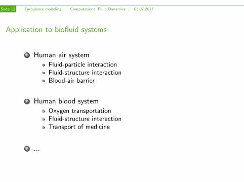
Application to biofluid systems
1 Human air system
Fluid-particle interactionFluid-structure interactionBlood-air barrier
2 Human blood system
Oxygen transportationFluid-structure interactionTransport of medicine
3 ...
Seite 12 Turbulence modeling | Computational Fluid Dynamics | 03.07.2017
Application to biofluid systems
1 Human air system
Fluid-particle interactionFluid-structure interactionBlood-air barrier
2 Human blood system
Oxygen transportationFluid-structure interactionTransport of medicine
3 ...

Seite 12 Turbulence modeling | Computational Fluid Dynamics | 03.07.2017
Application to biofluid systems
1 Human air system
Fluid-particle interactionFluid-structure interactionBlood-air barrier
2 Human blood system
Oxygen transportationFluid-structure interactionTransport of medicine
3 ...
Seite 12 Turbulence modeling | Computational Fluid Dynamics | 03.07.2017
Application to biofluid systems
1 Human air system
Fluid-particle interactionFluid-structure interactionBlood-air barrier
2 Human blood system
Oxygen transportationFluid-structure interactionTransport of medicine
3 ...

Seite 13 Turbulence modeling | Computational Fluid Dynamics | 03.07.2017
Break
5 min
Seite 14 Review | Computational Fluid Dynamics | 03.07.2017
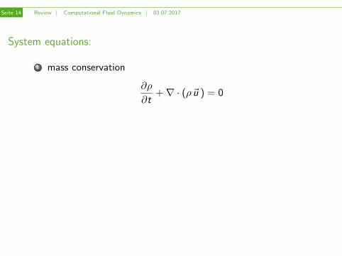
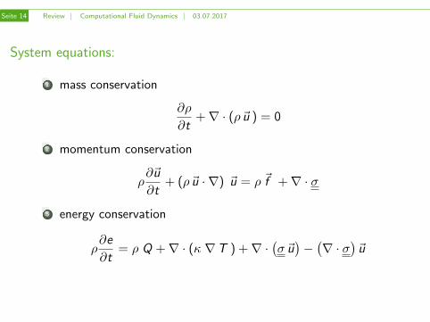
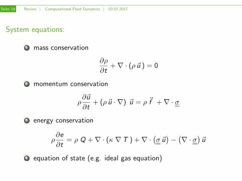
System equations:
1 mass conservation
∂ρ
∂t+∇ · (ρ~u ) = 0
2 momentum conservation
ρ∂~u
∂t+ (ρ~u · ∇) ~u = ρ ~f +∇ · σ
3 energy conservation
ρ∂e
∂t= ρ Q +∇ · (κ ∇T ) +∇ ·
(σ~u)−(∇ · σ
)~u
4 equation of state (e.g. ideal gas equation)

Seite 14 Review | Computational Fluid Dynamics | 03.07.2017
System equations:
1 mass conservation
∂ρ
∂t+∇ · (ρ~u ) = 0
2 momentum conservation
ρ∂~u
∂t+ (ρ~u · ∇) ~u = ρ ~f +∇ · σ
3 energy conservation
ρ∂e
∂t= ρ Q +∇ · (κ ∇T ) +∇ ·
(σ~u)−(∇ · σ
)~u
4 equation of state (e.g. ideal gas equation)
Seite 14 Review | Computational Fluid Dynamics | 03.07.2017
System equations:
1 mass conservation
∂ρ
∂t+∇ · (ρ~u ) = 0
2 momentum conservation
ρ∂~u
∂t+ (ρ~u · ∇) ~u = ρ ~f +∇ · σ
3 energy conservation
ρ∂e
∂t= ρ Q +∇ · (κ ∇T ) +∇ ·
(σ~u)−(∇ · σ
)~u
4 equation of state (e.g. ideal gas equation)
Seite 14 Review | Computational Fluid Dynamics | 03.07.2017
System equations:
1 mass conservation
∂ρ
∂t+∇ · (ρ~u ) = 0
2 momentum conservation
ρ∂~u
∂t+ (ρ~u · ∇) ~u = ρ ~f +∇ · σ
3 energy conservation
ρ∂e
∂t= ρ Q +∇ · (κ ∇T ) +∇ ·
(σ~u)−(∇ · σ
)~u
4 equation of state (e.g. ideal gas equation)
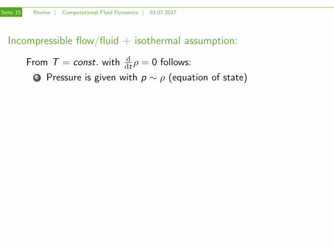
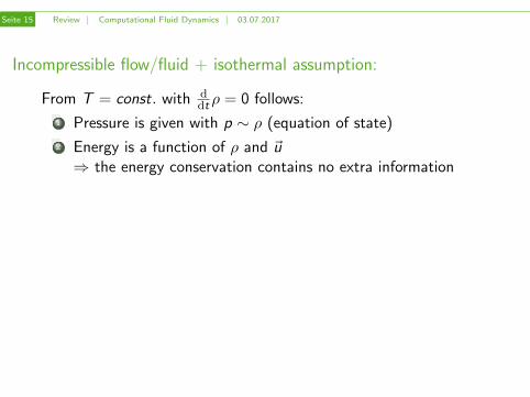
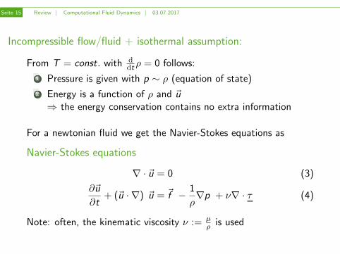
Seite 15 Review | Computational Fluid Dynamics | 03.07.2017
Incompressible flow/fluid + isothermal assumption:
From T = const. with ddt ρ = 0 follows:
1 Pressure is given with p ∼ ρ (equation of state)
2 Energy is a function of ρ and ~u⇒ the energy conservation contains no extra information
For a newtonian fluid we get the Navier-Stokes equations as
Navier-Stokes equations
∇ · ~u = 0 (3)
∂~u
∂t+ (~u · ∇) ~u = ~f − 1
ρ∇p + ν∇ · τ (4)
Note: often, the kinematic viscosity ν := µρ is used
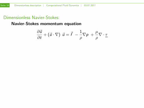
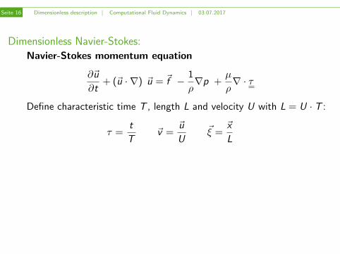
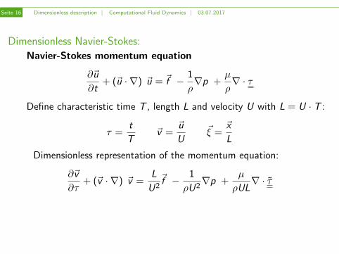
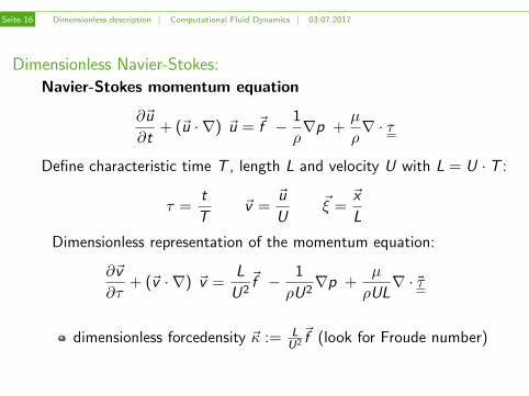
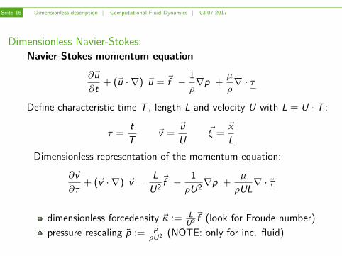
Seite 16 Dimensionless description | Computational Fluid Dynamics | 03.07.2017
Dimensionless Navier-Stokes:
Navier-Stokes momentum equation
∂~u
∂t+ (~u · ∇) ~u = ~f − 1
ρ∇p +
µ
ρ∇ · τ
Define characteristic time T , length L and velocity U with L = U · T :
τ =t
T~v =
~u
U~ξ =
~x
L
Dimensionless representation of the momentum equation:
∂~v
∂τ+ (~v · ∇) ~v =
L
U2~f − 1
ρU2∇p +
µ
ρUL∇ · τ
dimensionless forcedensity ~κ := LU2~f (look for Froude number)
pressure rescaling p := pρU2 (NOTE: only for inc. fluid)
Seite 17 Dimensionless description | Computational Fluid Dynamics | 03.07.2017
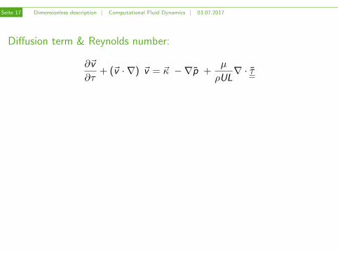
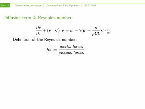
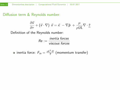
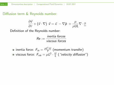
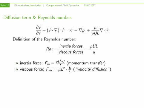
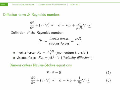
Diffusion term & Reynolds number:
∂~v
∂τ+ (~v · ∇) ~v = ~κ −∇p +
µ
ρUL∇ · τ
Definition of the Reynolds number:
Re :=inertia forces
viscous forces
=ρUL
µ
inertia force: Fin = ρL3·UT (momentum transfer)
viscous force: Fvis = µL2 · UL (“velocity diffusion”)
Dimensionless Navier-Stokes equations
∇ · ~v = 0 (5)
∂~v
∂τ+ (~v · ∇) ~v = ~κ −∇p +
1
Re∇ · τ (6)
Seite 17 Dimensionless description | Computational Fluid Dynamics | 03.07.2017
Diffusion term & Reynolds number:
∂~v
∂τ+ (~v · ∇) ~v = ~κ −∇p +
µ
ρUL∇ · τ
Definition of the Reynolds number:
Re :=inertia forces
viscous forces=ρUL
µ
inertia force: Fin = ρL3·UT (momentum transfer)
viscous force: Fvis = µL2 · UL (“velocity diffusion”)
Dimensionless Navier-Stokes equations
∇ · ~v = 0 (5)
∂~v
∂τ+ (~v · ∇) ~v = ~κ −∇p +
1
Re∇ · τ (6)
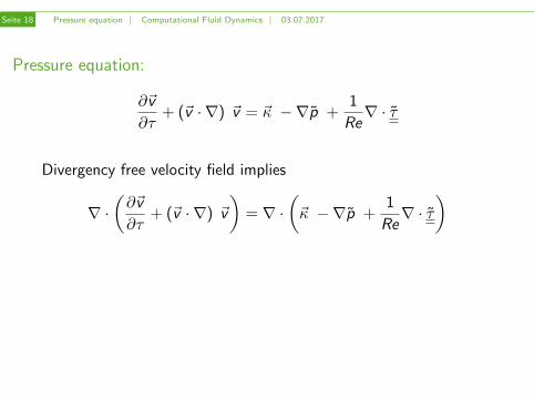
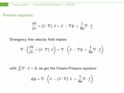
Seite 18 Pressure equation | Computational Fluid Dynamics | 03.07.2017
Pressure equation:
∂~v
∂τ+ (~v · ∇) ~v = ~κ −∇p +
1
Re∇ · τ
Divergency free velocity field implies
∇ ·(∂~v
∂τ+ (~v · ∇) ~v
)= ∇ ·
(~κ −∇p +
1
Re∇ · τ
)
with ∂∂τ∇ · ~v = 0, we get the Poissin-Pressure equation:
∆p = ∇ ·(~κ − (~v · ∇) ~v +
1
Re∇ · τ
)

Seite 19 Turbulent flow | Computational Fluid Dynamics | 03.07.2017
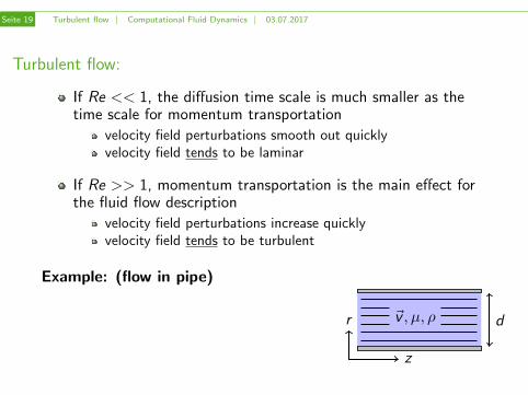
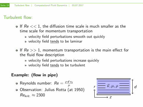
Turbulent flow:
If Re << 1, the diffusion time scale is much smaller as thetime scale for momentum transportation
velocity field perturbations smooth out quicklyvelocity field tends to be laminar
If Re >> 1, momentum transportation is the main effect forthe fluid flow description
velocity field perturbations increase quicklyvelocity field tends to be turbulent
Example: (flow in pipe)
Reynolds number: Re = ρ d vzµ
Observation: Julius Rotta (at 1950)Rekrit. ≈ 2300
~v , µ, ρ dr
z

Seite 19 Turbulent flow | Computational Fluid Dynamics | 03.07.2017
Turbulent flow:
If Re << 1, the diffusion time scale is much smaller as thetime scale for momentum transportation
velocity field perturbations smooth out quicklyvelocity field tends to be laminar
If Re >> 1, momentum transportation is the main effect forthe fluid flow description
velocity field perturbations increase quicklyvelocity field tends to be turbulent
Example: (flow in pipe)
Reynolds number: Re = ρ d vzµ
Observation: Julius Rotta (at 1950)Rekrit. ≈ 2300
~v , µ, ρ dr
z
Seite 20 Turbulent flow | Computational Fluid Dynamics | 03.07.2017
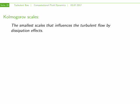
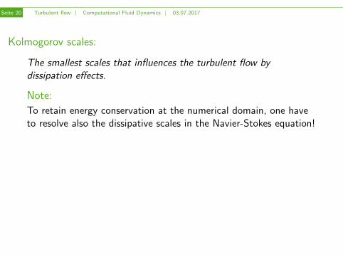
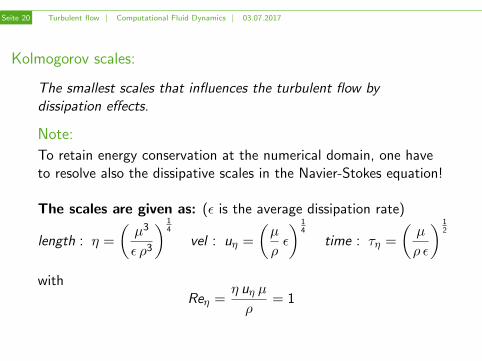
Kolmogorov scales:
The smallest scales that influences the turbulent flow bydissipation effects.
Note:
To retain energy conservation at the numerical domain, one haveto resolve also the dissipative scales in the Navier-Stokes equation!
The scales are given as: (ε is the average dissipation rate)
length : η =
(µ3
ε ρ3
) 14
vel : uη =
(µ
ρε
) 14
time : τη =
(µ
ρ ε
) 12
withReη =
η uη µ
ρ= 1
Seite 20 Turbulent flow | Computational Fluid Dynamics | 03.07.2017
Kolmogorov scales:
The smallest scales that influences the turbulent flow bydissipation effects.
Note:
To retain energy conservation at the numerical domain, one haveto resolve also the dissipative scales in the Navier-Stokes equation!
The scales are given as: (ε is the average dissipation rate)
length : η =
(µ3
ε ρ3
) 14
vel : uη =
(µ
ρε
) 14
time : τη =
(µ
ρ ε
) 12
withReη =
η uη µ
ρ= 1
Seite 21 Turbulence models | Computational Fluid Dynamics | 03.07.2017
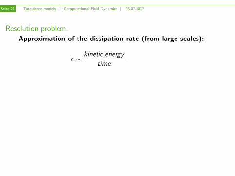
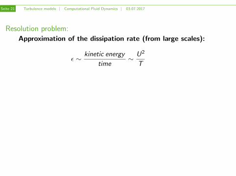
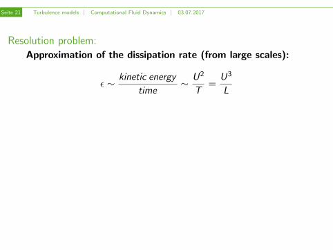
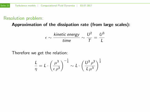
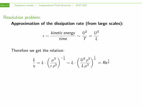
Resolution problem:
Approximation of the dissipation rate (from large scales):
ε ∼ kinetic energy
time
∼ U2
T=
U3
L
Therefore we get the relation:
L
η= L ·
(µ3
ε ρ3
)− 14
∼ L ·(
U3 ρ3
Lµ3
) 14
= Re34
Example: (L ≈ 103m , v ≈ 1 ms , ρ ≈ 1.3 kg
m3 , µ ≈ 17.1 µPa · s)
Re ≈ 7.5 · 109
η ≈ 4 · 10−5 m
Seite 21 Turbulence models | Computational Fluid Dynamics | 03.07.2017
Resolution problem:
Approximation of the dissipation rate (from large scales):
ε ∼ kinetic energy
time∼ U2
T
=U3
L
Therefore we get the relation:
L
η= L ·
(µ3
ε ρ3
)− 14
∼ L ·(
U3 ρ3
Lµ3
) 14
= Re34
Example: (L ≈ 103m , v ≈ 1 ms , ρ ≈ 1.3 kg
m3 , µ ≈ 17.1 µPa · s)
Re ≈ 7.5 · 109
η ≈ 4 · 10−5 m
Seite 21 Turbulence models | Computational Fluid Dynamics | 03.07.2017
Resolution problem:
Approximation of the dissipation rate (from large scales):
ε ∼ kinetic energy
time∼ U2
T=
U3
L
Therefore we get the relation:
L
η= L ·
(µ3
ε ρ3
)− 14
∼ L ·(
U3 ρ3
Lµ3
) 14
= Re34
Example: (L ≈ 103m , v ≈ 1 ms , ρ ≈ 1.3 kg
m3 , µ ≈ 17.1 µPa · s)
Re ≈ 7.5 · 109
η ≈ 4 · 10−5 m
Seite 21 Turbulence models | Computational Fluid Dynamics | 03.07.2017
Resolution problem:
Approximation of the dissipation rate (from large scales):
ε ∼ kinetic energy
time∼ U2
T=
U3
L
Therefore we get the relation:
L
η= L ·
(µ3
ε ρ3
)− 14
∼ L ·(
U3 ρ3
Lµ3
) 14
= Re34
Example: (L ≈ 103m , v ≈ 1 ms , ρ ≈ 1.3 kg
m3 , µ ≈ 17.1 µPa · s)
Re ≈ 7.5 · 109
η ≈ 4 · 10−5 m
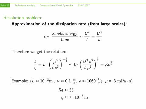
Seite 22 Turbulence models | Computational Fluid Dynamics | 03.07.2017
Resolution problem:
Approximation of the dissipation rate (from large scales):
ε ∼ kinetic energy
time∼ U2
T=
U3
L
Therefore we get the relation:
L
η= L ·
(µ3
ε ρ3
)− 14
∼ L ·(
U3 ρ3
Lµ3
) 14
= Re34
Example: (L ≈ 10−3m , v ≈ 0.1 ms , ρ ≈ 1060 kg
m3 , µ ≈ 3 mPa · s)
Re ≈ 35
η ≈ 7 · 10−5 m
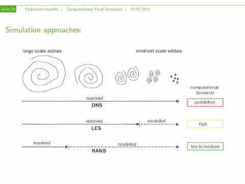
Seite 23 Turbulence models | Computational Fluid Dynamics | 03.07.2017
Simulation approaches:
Seite 24 Turbulence models | Computational Fluid Dynamics | 03.07.2017
Simulation approaches:
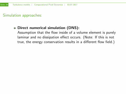
Direct numerical simulation (DNS):Assumption that the flow inside of a volume element is purelylaminar and no dissipation effect occurs. (Note: If this is nottrue, the energy conservation results in a different flow field.)
Eddy dissipation modelling on small scales:Reynolds-Averaged Navier Stokes (RANS)Large-Eddy Simulation...
v = 〈v〉+ v ′ and p = 〈p〉+ p′
with the mean value 〈·〉 of · and the fluctuating part ·′.

Seite 24 Turbulence models | Computational Fluid Dynamics | 03.07.2017
Simulation approaches:
Direct numerical simulation (DNS):Assumption that the flow inside of a volume element is purelylaminar and no dissipation effect occurs. (Note: If this is nottrue, the energy conservation results in a different flow field.)
Eddy dissipation modelling on small scales:Reynolds-Averaged Navier Stokes (RANS)Large-Eddy Simulation...
v = 〈v〉+ v ′ and p = 〈p〉+ p′
with the mean value 〈·〉 of · and the fluctuating part ·′.
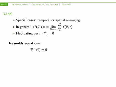
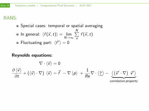
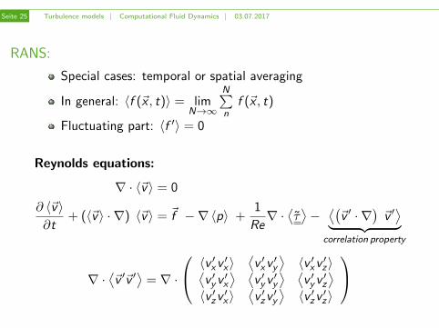
Seite 25 Turbulence models | Computational Fluid Dynamics | 03.07.2017
RANS:
Special cases: temporal or spatial averaging
In general: 〈f (~x , t)〉 = limN→∞
N∑n
f (~x , t)
Fluctuating part: 〈f ′〉 = 0
Reynolds equations:
∇ · 〈~v〉 = 0
∂ 〈~v〉∂t
+ (〈~v〉 · ∇) 〈~v〉 = ~f −∇〈p〉 +1
Re∇ ·⟨τ⟩−⟨(~v ′ · ∇
)~v ′⟩︸ ︷︷ ︸
correlation property
∇ ·⟨~v ′~v ′
⟩= ∇ ·
〈v ′xv ′x〉⟨v ′xv ′y
⟩〈v ′xv ′z〉⟨
v ′yv ′x⟩ ⟨
v ′yv ′y⟩ ⟨
v ′yv ′z⟩
〈v ′zv ′x〉⟨v ′zv ′y
⟩〈v ′zv ′z〉
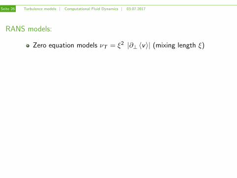
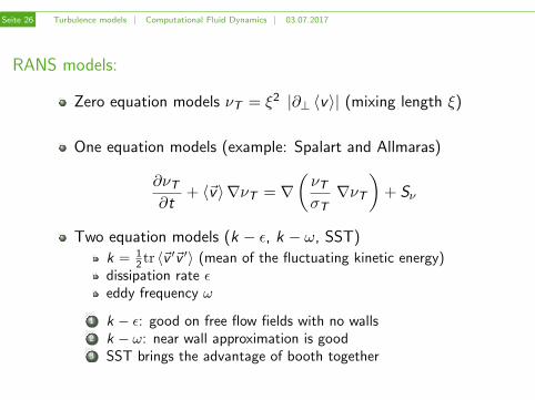
Seite 26 Turbulence models | Computational Fluid Dynamics | 03.07.2017
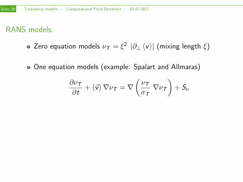
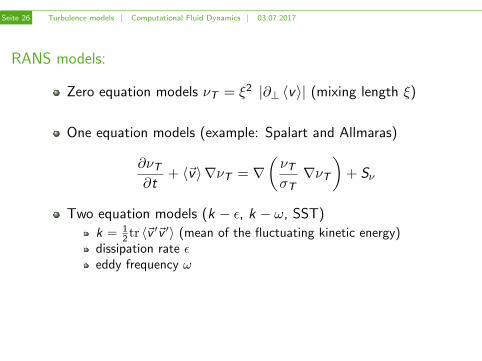
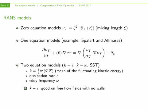
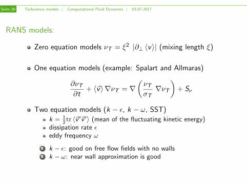
RANS models:
Zero equation models νT = ξ2 |∂⊥ 〈v〉| (mixing length ξ)
One equation models (example: Spalart and Allmaras)
∂νT∂t
+ 〈~v〉∇νT = ∇(νTσT∇νT
)+ Sν
Two equation models (k − ε, k − ω, SST)
k = 12 tr 〈~v
′~v ′〉 (mean of the fluctuating kinetic energy)dissipation rate εeddy frequency ω
1 k − ε: good on free flow fields with no walls2 k − ω: near wall approximation is good3 SST brings the advantage of booth together
Seite 26 Turbulence models | Computational Fluid Dynamics | 03.07.2017
RANS models:
Zero equation models νT = ξ2 |∂⊥ 〈v〉| (mixing length ξ)
One equation models (example: Spalart and Allmaras)
∂νT∂t
+ 〈~v〉∇νT = ∇(νTσT∇νT
)+ Sν
Two equation models (k − ε, k − ω, SST)
k = 12 tr 〈~v
′~v ′〉 (mean of the fluctuating kinetic energy)dissipation rate εeddy frequency ω
1 k − ε: good on free flow fields with no walls
2 k − ω: near wall approximation is good3 SST brings the advantage of booth together
Seite 26 Turbulence models | Computational Fluid Dynamics | 03.07.2017
RANS models:
Zero equation models νT = ξ2 |∂⊥ 〈v〉| (mixing length ξ)
One equation models (example: Spalart and Allmaras)
∂νT∂t
+ 〈~v〉∇νT = ∇(νTσT∇νT
)+ Sν
Two equation models (k − ε, k − ω, SST)
k = 12 tr 〈~v
′~v ′〉 (mean of the fluctuating kinetic energy)dissipation rate εeddy frequency ω
1 k − ε: good on free flow fields with no walls2 k − ω: near wall approximation is good
3 SST brings the advantage of booth together
Seite 26 Turbulence models | Computational Fluid Dynamics | 03.07.2017
RANS models:
Zero equation models νT = ξ2 |∂⊥ 〈v〉| (mixing length ξ)
One equation models (example: Spalart and Allmaras)
∂νT∂t
+ 〈~v〉∇νT = ∇(νTσT∇νT
)+ Sν
Two equation models (k − ε, k − ω, SST)
k = 12 tr 〈~v
′~v ′〉 (mean of the fluctuating kinetic energy)dissipation rate εeddy frequency ω
1 k − ε: good on free flow fields with no walls2 k − ω: near wall approximation is good3 SST brings the advantage of booth together
Seite 27 Turbulence models | Computational Fluid Dynamics | 03.07.2017
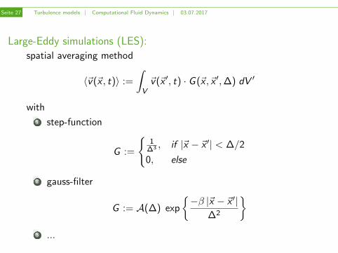
Large-Eddy simulations (LES):
spatial averaging method
〈~v(~x , t)〉 :=
∫V~v(~x ′, t) · G (~x ,~x ′,∆) dV ′
with
1 step-function
G :=
1
∆3 , if |~x − ~x ′| < ∆/2
0, else
2 gauss-filter
G := A(∆) exp
−β |~x − ~x ′|
∆2
3 ...
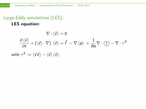
Seite 28 Turbulence models | Computational Fluid Dynamics | 03.07.2017
Large-Eddy simulations (LES):
LES equation:
∇ · 〈~v〉 = 0
∂ 〈~v〉∂t
+ (〈~v〉 · ∇) 〈~v〉 = ~f −∇〈p〉 +1
Re∇ ·⟨τ⟩−∇ · τS
with τS := 〈~v~v〉 − 〈~v〉 〈~v〉.
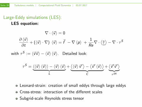
Detailed look:
τS = 〈〈~v〉 〈~v〉〉 − 〈~v〉 〈~v〉︸ ︷︷ ︸L
+⟨〈~v〉~v ′
⟩−⟨~v ′ 〈~v〉
⟩︸ ︷︷ ︸C
+⟨~v ′~v ′
⟩︸ ︷︷ ︸τSR
Leonard-strain: creation of small eddys through large eddys
Cross-stress: interaction of the different scales
Subgrid-scale Reynolds stress tensor
Seite 28 Turbulence models | Computational Fluid Dynamics | 03.07.2017
Large-Eddy simulations (LES):
LES equation:
∇ · 〈~v〉 = 0
∂ 〈~v〉∂t
+ (〈~v〉 · ∇) 〈~v〉 = ~f −∇〈p〉 +1
Re∇ ·⟨τ⟩−∇ · τS
with τS := 〈~v~v〉 − 〈~v〉 〈~v〉. Detailed look:
τS = 〈〈~v〉 〈~v〉〉 − 〈~v〉 〈~v〉︸ ︷︷ ︸L
+⟨〈~v〉~v ′
⟩−⟨~v ′ 〈~v〉
⟩︸ ︷︷ ︸C
+⟨~v ′~v ′
⟩︸ ︷︷ ︸τSR
Leonard-strain: creation of small eddys through large eddys
Cross-stress: interaction of the different scales
Subgrid-scale Reynolds stress tensor

Seite 29 Turbulence models | Computational Fluid Dynamics | 03.07.2017
Break
5 min

Seite 30 Practical application | Computational Fluid Dynamics | 03.07.2017
Application

Seite 31 Practical application | Computational Fluid Dynamics | 03.07.2017
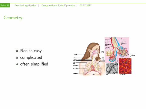
Geometry
Not as easy
complicated
often simplified

Seite 31 Practical application | Computational Fluid Dynamics | 03.07.2017
Geometry
Not as easy
complicated
often simplified

Seite 31 Practical application | Computational Fluid Dynamics | 03.07.2017
Geometry
Not as easy
complicated
often simplified
Seite 31 Practical application | Computational Fluid Dynamics | 03.07.2017
Geometry
Not as easy
complicated
often simplified

Seite 32 Practical application | Computational Fluid Dynamics | 03.07.2017
Application
Seite 33 Practical application | Computational Fluid Dynamics | 03.07.2017
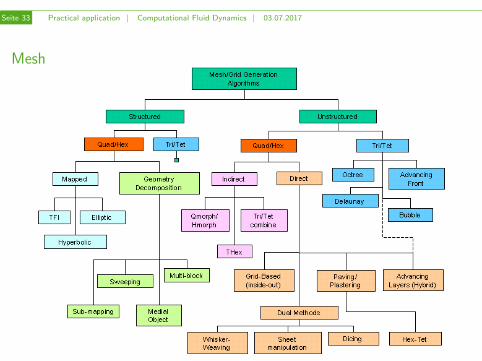
Mesh
Seite 34 Practical application | Computational Fluid Dynamics | 03.07.2017
Mesh
Mesh quality determined by:
area
aspect ratio
diagonal ratio
edge ratio
skewness
orthogonal quality
stretch
taper
volume
Seite 35 Practical application | Computational Fluid Dynamics | 03.07.2017
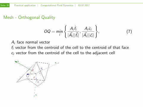
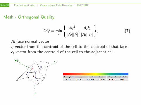
Mesh - Orthogonal Quality
OQ = mini
Ai fi
| ~Ai ||~fi |,
Ai ci
| ~Ai ||~ci |
, (7)
Ai face normal vectorfi vector from the centroid of the cell to the centroid of that faceci vector from the centroid of the cell to the adjacent cell
Seite 35 Practical application | Computational Fluid Dynamics | 03.07.2017
Mesh - Orthogonal Quality
OQ = mini
Ai fi
| ~Ai ||~fi |,
Ai ci
| ~Ai ||~ci |
, (7)
Ai face normal vectorfi vector from the centroid of the cell to the centroid of that faceci vector from the centroid of the cell to the adjacent cell
Seite 36 Practical application | Computational Fluid Dynamics | 03.07.2017
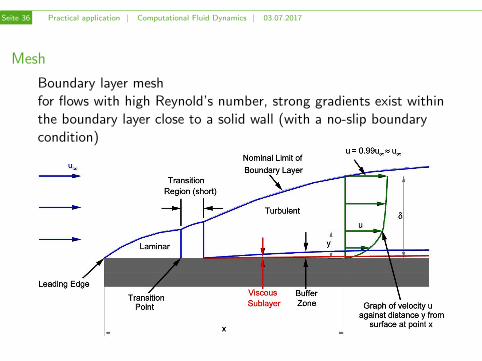
Mesh
Boundary layer meshfor flows with high Reynold’s number, strong gradients exist withinthe boundary layer close to a solid wall (with a no-slip boundarycondition)
Seite 36 Practical application | Computational Fluid Dynamics | 03.07.2017
Mesh
Boundary layer meshfor flows with high Reynold’s number, strong gradients exist withinthe boundary layer close to a solid wall (with a no-slip boundarycondition)
Seite 37 Practical application | Computational Fluid Dynamics | 03.07.2017
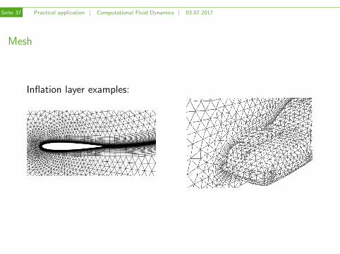
Mesh
Inflation layer examples:
Seite 38 Practical application | Computational Fluid Dynamics | 03.07.2017
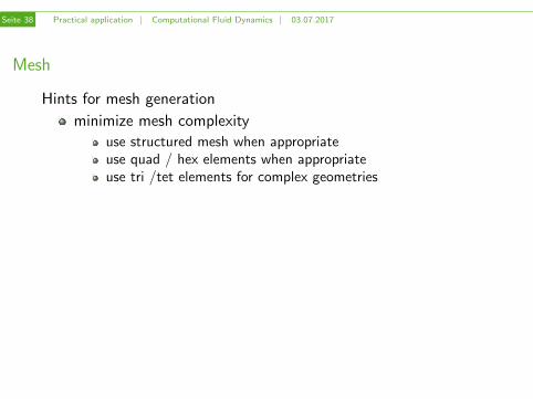
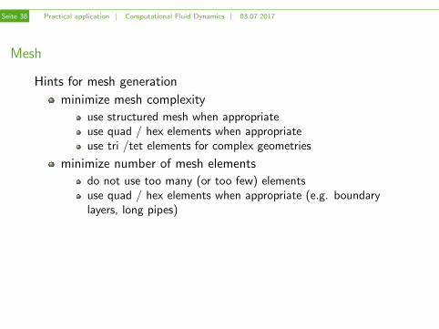
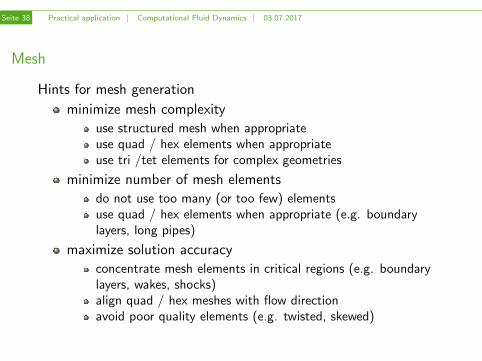
Mesh
Hints for mesh generation
minimize mesh complexity
use structured mesh when appropriateuse quad / hex elements when appropriateuse tri /tet elements for complex geometries
minimize number of mesh elements
do not use too many (or too few) elementsuse quad / hex elements when appropriate (e.g. boundarylayers, long pipes)
maximize solution accuracy
concentrate mesh elements in critical regions (e.g. boundarylayers, wakes, shocks)align quad / hex meshes with flow directionavoid poor quality elements (e.g. twisted, skewed)
Seite 38 Practical application | Computational Fluid Dynamics | 03.07.2017
Mesh
Hints for mesh generation
minimize mesh complexity
use structured mesh when appropriateuse quad / hex elements when appropriateuse tri /tet elements for complex geometries
minimize number of mesh elements
do not use too many (or too few) elementsuse quad / hex elements when appropriate (e.g. boundarylayers, long pipes)
maximize solution accuracy
concentrate mesh elements in critical regions (e.g. boundarylayers, wakes, shocks)align quad / hex meshes with flow directionavoid poor quality elements (e.g. twisted, skewed)
Seite 39 Practical application | Computational Fluid Dynamics | 03.07.2017
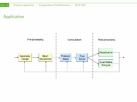
Application
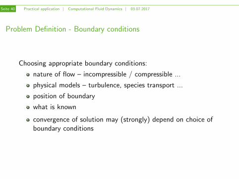
Seite 40 Practical application | Computational Fluid Dynamics | 03.07.2017
Problem Definition - Boundary conditions
Choosing appropriate boundary conditions:
nature of flow – incompressible / compressible ...
physical models – turbulence, species transport ...
position of boundary
what is known
convergence of solution may (strongly) depend on choice ofboundary conditions
Seite 41 Practical application | Computational Fluid Dynamics | 03.07.2017
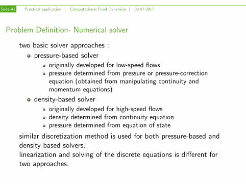
Problem Definition- Numerical solver
two basic solver approaches :
pressure-based solver
originally developed for low-speed flowspressure determined from pressure or pressure-correctionequation (obtained from manipulating continuity andmomentum equations)
density-based solver
originally developed for high-speed flowsdensity determined from continuity equationpressure determined from equation of state
similar discretization method is used for both pressure-based anddensity-based solvers.linearization and solving of the discrete equations is different fortwo approaches.

Seite 42 Practical application | Computational Fluid Dynamics | 03.07.2017
Application
Seite 43 Practical application | Computational Fluid Dynamics | 03.07.2017
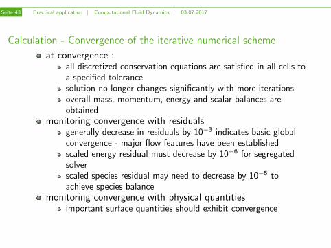
Calculation - Convergence of the iterative numerical scheme
at convergence :all discretized conservation equations are satisfied in all cells toa specified tolerancesolution no longer changes significantly with more iterationsoverall mass, momentum, energy and scalar balances areobtained
monitoring convergence with residuals
generally decrease in residuals by 10−3 indicates basic globalconvergence - major flow features have been establishedscaled energy residual must decrease by 10−6 for segregatedsolverscaled species residual may need to decrease by 10−5 toachieve species balance
monitoring convergence with physical quantities
important surface quantities should exhibit convergence
checking for property conservation
overall heat and mass balances should be within 0.1% of netflux through domain

Seite 43 Practical application | Computational Fluid Dynamics | 03.07.2017
Calculation - Convergence of the iterative numerical scheme
at convergence :all discretized conservation equations are satisfied in all cells toa specified tolerancesolution no longer changes significantly with more iterationsoverall mass, momentum, energy and scalar balances areobtained
monitoring convergence with residualsgenerally decrease in residuals by 10−3 indicates basic globalconvergence - major flow features have been establishedscaled energy residual must decrease by 10−6 for segregatedsolverscaled species residual may need to decrease by 10−5 toachieve species balance
monitoring convergence with physical quantities
important surface quantities should exhibit convergence
checking for property conservation
overall heat and mass balances should be within 0.1% of netflux through domain
Seite 43 Practical application | Computational Fluid Dynamics | 03.07.2017
Calculation - Convergence of the iterative numerical scheme
at convergence :all discretized conservation equations are satisfied in all cells toa specified tolerancesolution no longer changes significantly with more iterationsoverall mass, momentum, energy and scalar balances areobtained
monitoring convergence with residualsgenerally decrease in residuals by 10−3 indicates basic globalconvergence - major flow features have been establishedscaled energy residual must decrease by 10−6 for segregatedsolverscaled species residual may need to decrease by 10−5 toachieve species balance
monitoring convergence with physical quantitiesimportant surface quantities should exhibit convergence
checking for property conservation
overall heat and mass balances should be within 0.1% of netflux through domain

Seite 43 Practical application | Computational Fluid Dynamics | 03.07.2017
Calculation - Convergence of the iterative numerical scheme
at convergence :all discretized conservation equations are satisfied in all cells toa specified tolerancesolution no longer changes significantly with more iterationsoverall mass, momentum, energy and scalar balances areobtained
monitoring convergence with residualsgenerally decrease in residuals by 10−3 indicates basic globalconvergence - major flow features have been establishedscaled energy residual must decrease by 10−6 for segregatedsolverscaled species residual may need to decrease by 10−5 toachieve species balance
monitoring convergence with physical quantitiesimportant surface quantities should exhibit convergence
checking for property conservationoverall heat and mass balances should be within 0.1% of netflux through domain
Seite 44 Practical application | Computational Fluid Dynamics | 03.07.2017
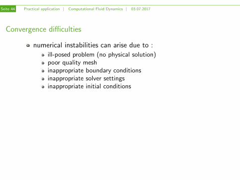
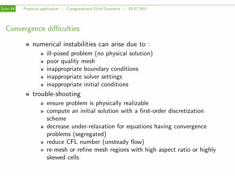
Convergence difficulties
numerical instabilities can arise due to :
ill-posed problem (no physical solution)poor quality meshinappropriate boundary conditionsinappropriate solver settingsinappropriate initial conditions
trouble-shooting
ensure problem is physically realizablecompute an initial solution with a first-order discretizationschemedecrease under-relaxation for equations having convergenceproblems (segregated)reduce CFL number (unsteady flow)re-mesh or refine mesh regions with high aspect ratio or highlyskewed cells
Seite 44 Practical application | Computational Fluid Dynamics | 03.07.2017
Convergence difficulties
numerical instabilities can arise due to :
ill-posed problem (no physical solution)poor quality meshinappropriate boundary conditionsinappropriate solver settingsinappropriate initial conditions
trouble-shooting
ensure problem is physically realizablecompute an initial solution with a first-order discretizationschemedecrease under-relaxation for equations having convergenceproblems (segregated)reduce CFL number (unsteady flow)re-mesh or refine mesh regions with high aspect ratio or highlyskewed cells

Seite 45 Practical application | Computational Fluid Dynamics | 03.07.2017
Application
Seite 46 Practical application | Computational Fluid Dynamics | 03.07.2017
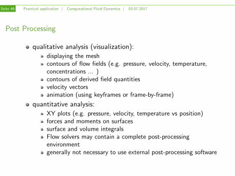
Post Processing
qualitative analysis (visualization):
displaying the meshcontours of flow fields (e.g. pressure, velocity, temperature,concentrations ... )contours of derived field quantitiesvelocity vectorsanimation (using keyframes or frame-by-frame)
quantitative analysis:
XY plots (e.g. pressure, velocity, temperature vs position)forces and moments on surfacessurface and volume integralsFlow solvers may contain a complete post-processingenvironmentgenerally not necessary to use external post-processing software

Seite 47 Practical application | Computational Fluid Dynamics | 03.07.2017
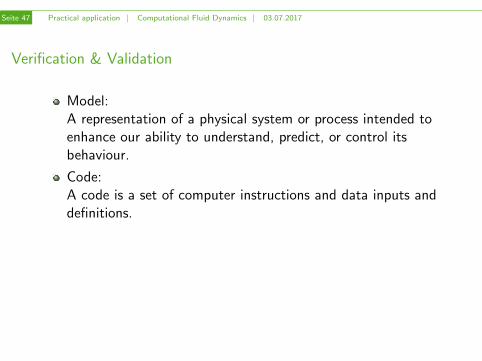
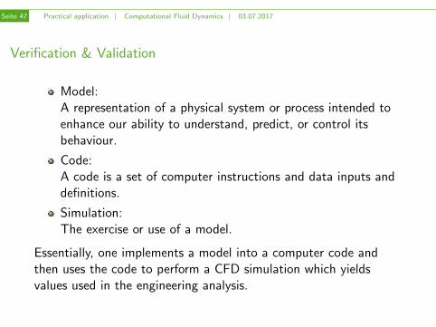
Verification & Validation
Model:A representation of a physical system or process intended toenhance our ability to understand, predict, or control itsbehaviour.
Code:A code is a set of computer instructions and data inputs anddefinitions.
Simulation:The exercise or use of a model.
Essentially, one implements a model into a computer code andthen uses the code to perform a CFD simulation which yieldsvalues used in the engineering analysis.
Seite 47 Practical application | Computational Fluid Dynamics | 03.07.2017
Verification & Validation
Model:A representation of a physical system or process intended toenhance our ability to understand, predict, or control itsbehaviour.
Code:A code is a set of computer instructions and data inputs anddefinitions.
Simulation:The exercise or use of a model.
Essentially, one implements a model into a computer code andthen uses the code to perform a CFD simulation which yieldsvalues used in the engineering analysis.
Seite 48 Practical application | Computational Fluid Dynamics | 03.07.2017
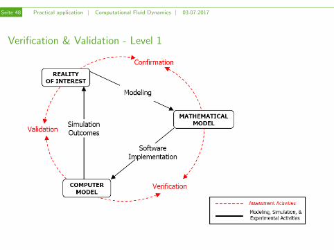
Verification & Validation - Level 1
Seite 49 Practical application | Computational Fluid Dynamics | 03.07.2017
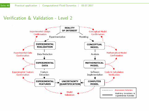
Verification & Validation - Level 2