![7. Heteroscedasticitylipas.uwasa.fi/~bepa/ecmc7.pdf · 2012-10-01 · 7.1 Consequences In the presence of heteroscedasticity: (i) OLS estimators are not BLUE (ii) Var[ ^ j]are biased,](https://static.fdocument.org/doc/165x107/5f77fc3d0b125015ba6f2530/7-het-bepaecmc7pdf-2012-10-01-71-consequences-in-the-presence-of-heteroscedasticity.jpg)
Forecasting based on creeping trend with harmonic weights Creeping trend can be used if variable...
28
Forecasting based on Forecasting based on creeping trend with creeping trend with harmonic weights harmonic weights Creeping trend can be used if variable changes irregularly in time. We use OLS to estimate parameters of partial trends.
-
Upload
jasper-lloyd -
Category
Documents
-
view
225 -
download
1
Transcript of Forecasting based on creeping trend with harmonic weights Creeping trend can be used if variable...
Forecasting based on creeping Forecasting based on creeping trend with harmonic weightstrend with harmonic weights
Creeping trend can be used if variable changes irregularly in time. We use OLS to estimate parameters of partial trends.
Step I
Determine the smoothing constant 1<k<n. The most often used k=3.
The quality of smoothing depends on the smoothing constant.
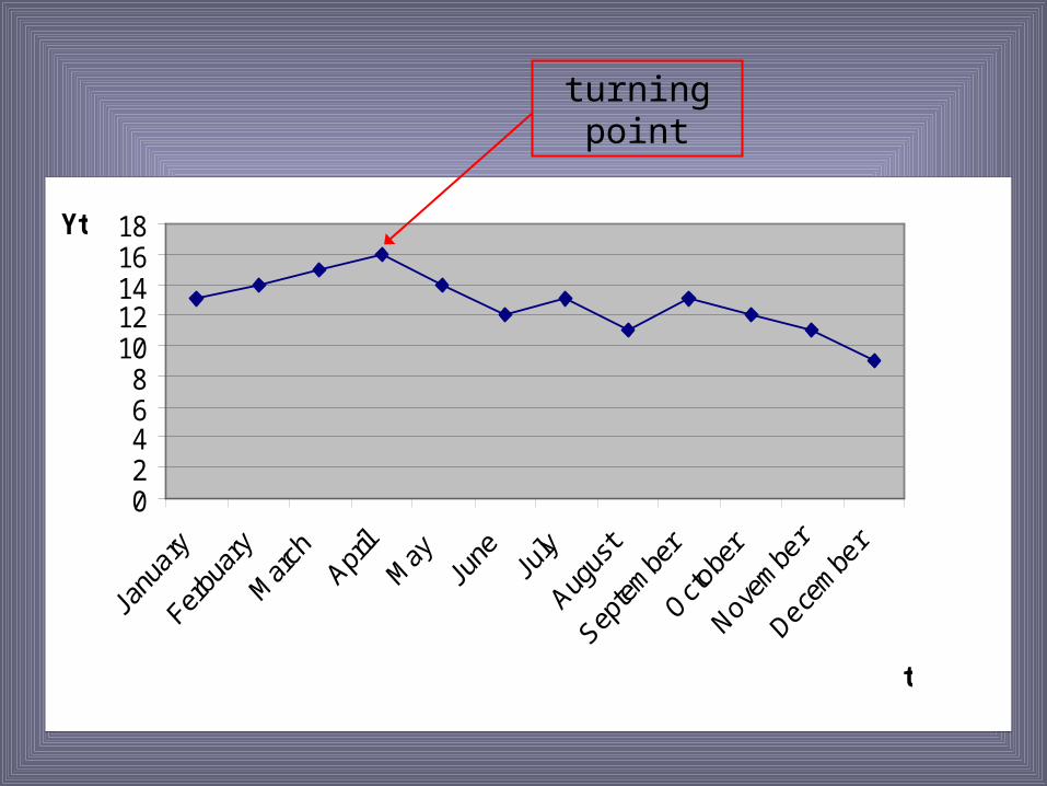
How to select the smoothing constant? Let’s have a look at your data. Detect the first turning point.
02468
1012141618
t
Yt
turning point
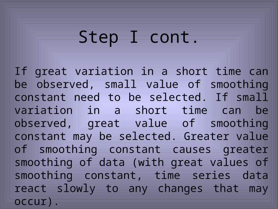
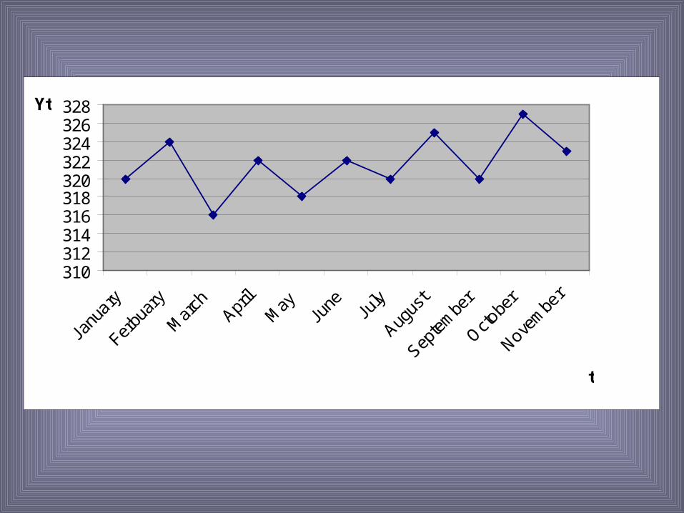
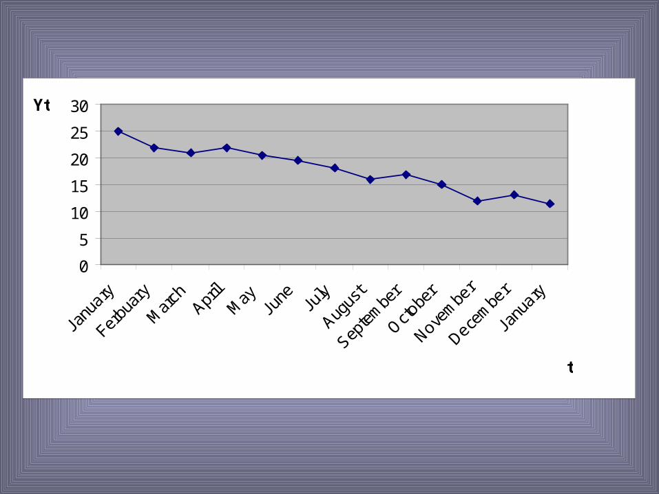
Step I cont.
If great variation in a short time can be observed, small value of smoothing constant need to be selected. If small variation in a short time can be observed, great value of smoothing constant may be selected. Greater value of smoothing constant causes greater smoothing of data (with great values of smoothing constant, time series data react slowly to any changes that may occur).
310312314316318320322324326328
January
Ferbuary
March
April
May
June Ju
ly
August
September
October
November
t
Yt
0
5
10
15
20
25
30
January
Ferbuary
March
April
May
June Ju
ly
August
September
October
November
December
January
t
Yt
Step II
Estimation of parameters with OLS for partial trends (smoothing constant, k, is the number of cases for each partial trend).
Step III
Determine smoothed values , (fitted values). For a given t from 2 to n-1, there is a set of approximants calculated from the partial trend equation.
ty
ty
Step IV
Determine mean smoothed value for t. Mean smoothed value is the mean of smoothed values for time period t.
ty~
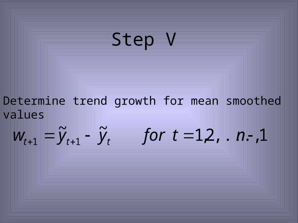
Step V
Determine trend growth for mean smoothed values
1,...,2,1~~11 ntforyyw ttt
Step VI
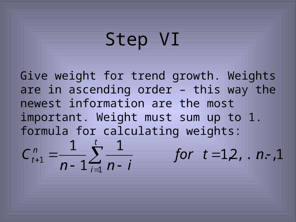
Give weight for trend growth. Weights are in ascending order – this way the newest information are the most important. Weight must sum up to 1. formula for calculating weights:
1,...,2,11
1
1
11
ntfor
innC
t
i
nt
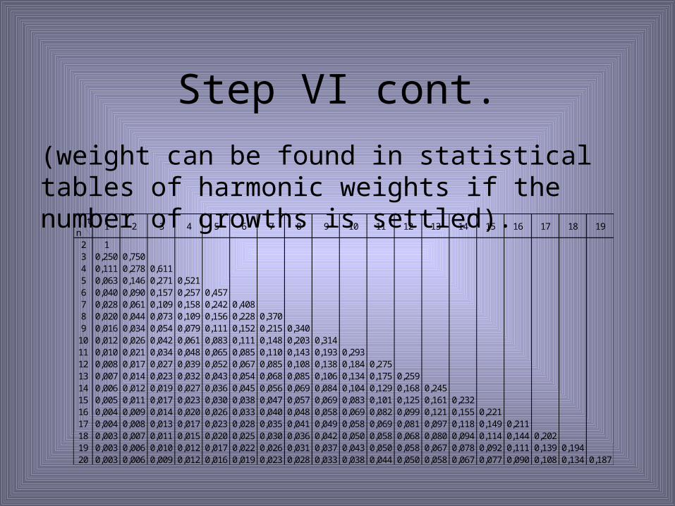
Step VI cont.
(weight can be found in statistical tables of harmonic weights if the number of growths is settled).
tn
10,250 0,7500,111 0,278 0,6110,063 0,146 0,271 0,5210,040 0,090 0,157 0,257 0,4570,028 0,061 0,109 0,158 0,242 0,4080,020 0,044 0,073 0,109 0,156 0,228 0,3700,016 0,034 0,054 0,079 0,111 0,152 0,215 0,3400,012 0,026 0,042 0,061 0,083 0,111 0,148 0,203 0,3140,010 0,021 0,034 0,048 0,065 0,085 0,110 0,143 0,193 0,2930,008 0,017 0,027 0,039 0,052 0,067 0,085 0,108 0,138 0,184 0,2750,007 0,014 0,023 0,032 0,043 0,054 0,068 0,085 0,106 0,134 0,175 0,2590,006 0,012 0,019 0,027 0,036 0,045 0,056 0,069 0,084 0,104 0,129 0,168 0,2450,005 0,011 0,017 0,023 0,030 0,038 0,047 0,057 0,069 0,083 0,101 0,125 0,161 0,2320,004 0,009 0,014 0,020 0,026 0,033 0,040 0,048 0,058 0,069 0,082 0,099 0,121 0,155 0,2210,004 0,008 0,013 0,017 0,023 0,028 0,035 0,041 0,049 0,058 0,069 0,081 0,097 0,118 0,149 0,2110,003 0,007 0,011 0,015 0,020 0,025 0,030 0,036 0,042 0,050 0,058 0,068 0,080 0,094 0,114 0,144 0,2020,003 0,006 0,010 0,012 0,017 0,022 0,026 0,031 0,037 0,043 0,050 0,058 0,067 0,078 0,092 0,111 0,139 0,1940,003 0,006 0,009 0,012 0,016 0,019 0,023 0,028 0,033 0,038 0,044 0,050 0,058 0,067 0,077 0,090 0,108 0,134 0,187
18 1913 14 15 1610 11 12 176 7 8 92 3 4 5
181920
1
14151617
10111213
6789
2345
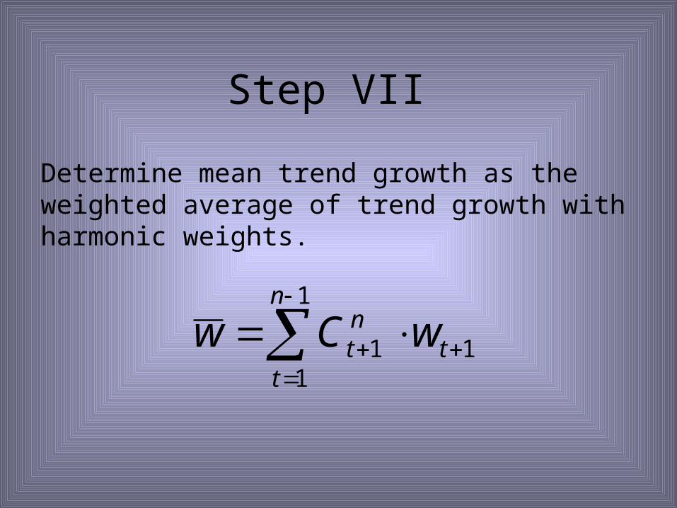
Step VII
Determine mean trend growth as the weighted average of trend growth with harmonic weights.
1
111
n
tt
nt wCw
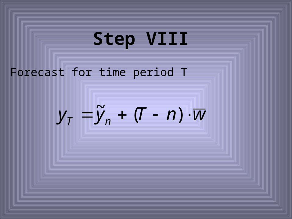
Step VIII
Forecast for time period T
wnTyy nT )(~
Step IX
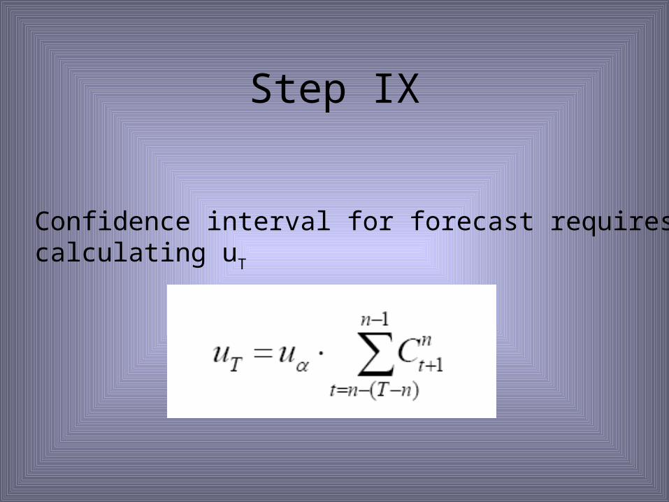
Confidence interval for forecast requires calculating uT
Step IX cont.
uα depends on normality of residuals.
1.If we didn’t reject the null hypothesis (residuals distribution is roughly normal), and n>30 u can be found in normal distribution tables. For sample size n<30 we should use t-Student distribution table (level of significance alpha and n-2 degrees of freedom)
Step IX cont.
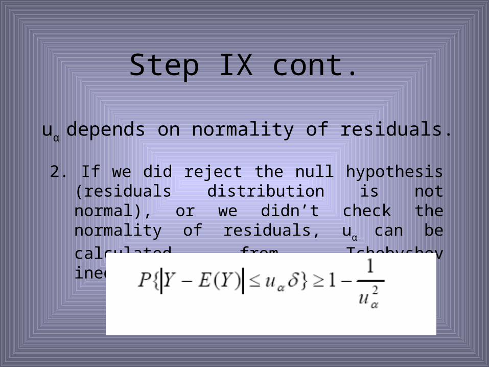
uα depends on normality of residuals.
2. If we did reject the null hypothesis (residuals distribution is not normal), or we didn’t check the normality of residuals, uα can be calculated from Tchebyshev
inequality:)
Step IX cont.
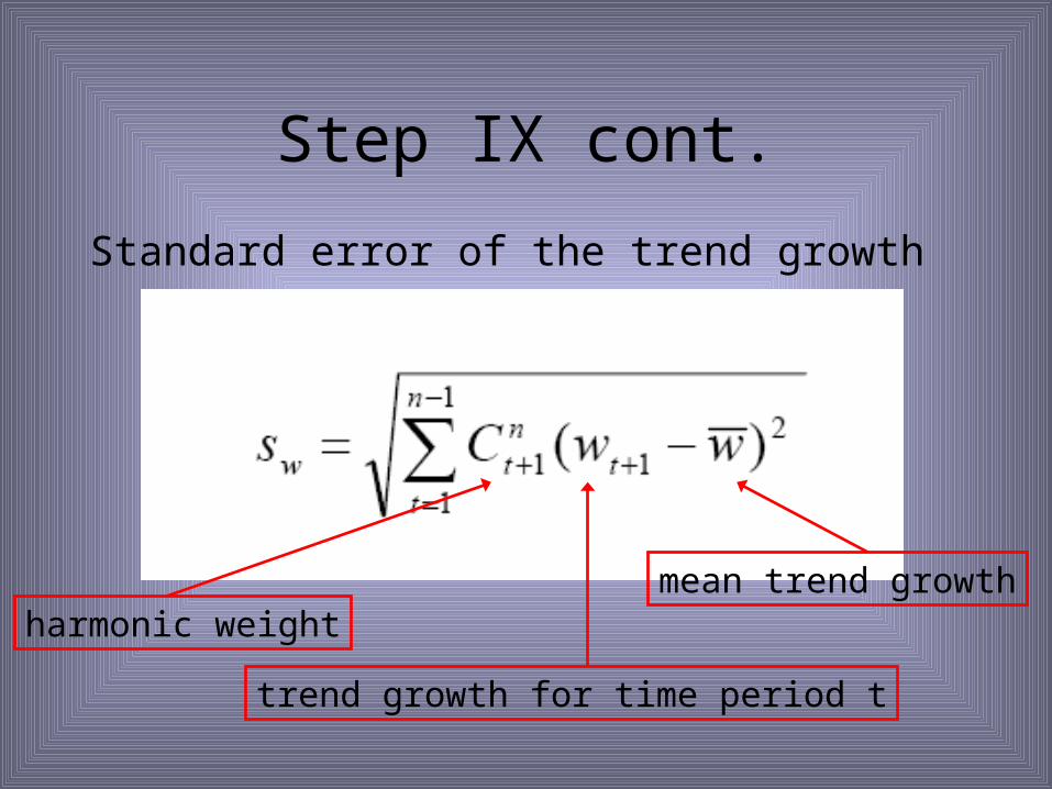
Standard error of the trend growth
harmonic weightmean trend growth
trend growth for time period t
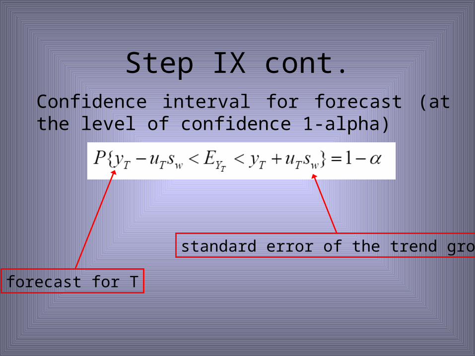
Step IX cont.Confidence interval for forecast (at the level of confidence 1-alpha)
forecast for T
standard error of the trend growth
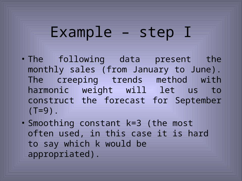
Example – step I
• The following data present the monthly sales (from January to June). The creeping trends method with harmonic weight will let us to construct the forecast for September (T=9).
• Smoothing constant k=3 (the most often used, in this case it is hard to say which k would be appropriated).
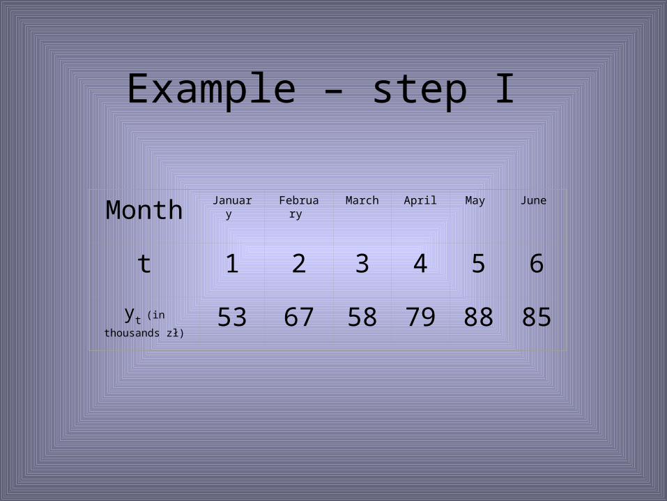
Example – step I
Month January February March April May June
t 1 2 3 4 5 6
yt (in
thousands zł)
53 67 58 79 88 85
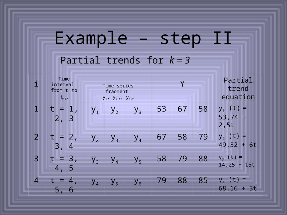
Example – step II
iTime
interval from ti to ti+2
Time series fragment yi, yi+1, yi+2
Y Partial trend equation
1 t = 1, 2, 3 y1 y2 y3 53 67 58 y1 (t) =
53,74 + 2,5t
2 t = 2, 3, 4 y2 y3 y4 67 58 79 y2 (t) = 49,32
+ 6t
3 t = 3, 4, 5 y3 y4 y5 58 79 88 y3 (t) = 14,25
+ 15t
4 t = 4, 5, 6 y4 y5 y6 79 88 85 y4 (t) = 68,16
+ 3t
Partial trends for k = 3
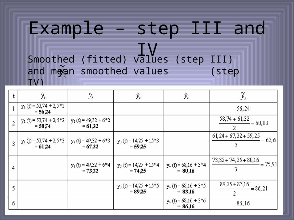
Example – step III and IVSmoothed (fitted) values (step III) and mean smoothed values (step IV) ty~
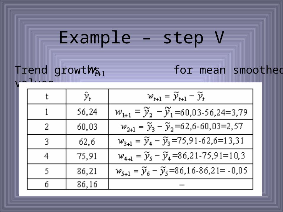
Example – step V
Trend growths for mean smoothed values 1tw
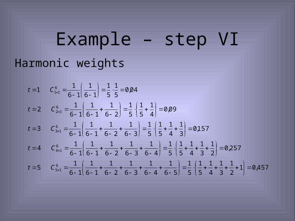
Example – step VIHarmonic weights
457,012
1
3
1
4
1
5
1
5
1
56
1
46
1
36
1
26
1
16
1
16
15
257,02
1
3
1
4
1
5
1
5
1
46
1
36
1
26
1
16
1
16
14
157,03
1
4
1
5
1
5
1
36
1
26
1
16
1
16
13
09,04
1
5
1
5
1
26
1
16
1
16
12
04,05
1
5
1
16
1
16
11
615
614
613
612
611
Ct
Ct
Ct
Ct
Ct
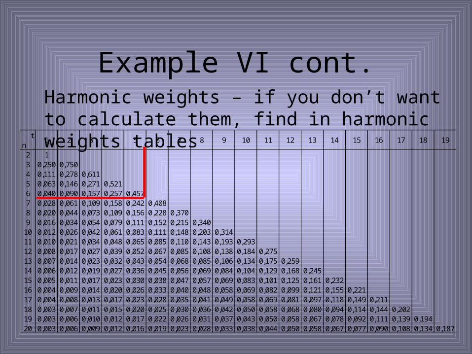
Example VI cont.Harmonic weights – if you don’t want to calculate them, find in harmonic weights tables
tn
10,250 0,7500,111 0,278 0,6110,063 0,146 0,271 0,5210,040 0,090 0,157 0,257 0,4570,028 0,061 0,109 0,158 0,242 0,4080,020 0,044 0,073 0,109 0,156 0,228 0,3700,016 0,034 0,054 0,079 0,111 0,152 0,215 0,3400,012 0,026 0,042 0,061 0,083 0,111 0,148 0,203 0,3140,010 0,021 0,034 0,048 0,065 0,085 0,110 0,143 0,193 0,2930,008 0,017 0,027 0,039 0,052 0,067 0,085 0,108 0,138 0,184 0,2750,007 0,014 0,023 0,032 0,043 0,054 0,068 0,085 0,106 0,134 0,175 0,2590,006 0,012 0,019 0,027 0,036 0,045 0,056 0,069 0,084 0,104 0,129 0,168 0,2450,005 0,011 0,017 0,023 0,030 0,038 0,047 0,057 0,069 0,083 0,101 0,125 0,161 0,2320,004 0,009 0,014 0,020 0,026 0,033 0,040 0,048 0,058 0,069 0,082 0,099 0,121 0,155 0,2210,004 0,008 0,013 0,017 0,023 0,028 0,035 0,041 0,049 0,058 0,069 0,081 0,097 0,118 0,149 0,2110,003 0,007 0,011 0,015 0,020 0,025 0,030 0,036 0,042 0,050 0,058 0,068 0,080 0,094 0,114 0,144 0,2020,003 0,006 0,010 0,012 0,017 0,022 0,026 0,031 0,037 0,043 0,050 0,058 0,067 0,078 0,092 0,111 0,139 0,1940,003 0,006 0,009 0,012 0,016 0,019 0,023 0,028 0,033 0,038 0,044 0,050 0,058 0,067 0,077 0,090 0,108 0,134 0,187
2345
1213
6789
181920
1
14151617
1011
2 3 4 5 6 7 8 9 10 11 12 17 18 1913 14 15 16
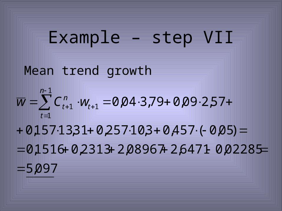
Example – step VII
Mean trend growth
097,5
02285,06471,208967,22313,01516,0
)05,0(457,03,10257,031,13157,0
57,209,079,304,01
111
n
tt
nt wCw
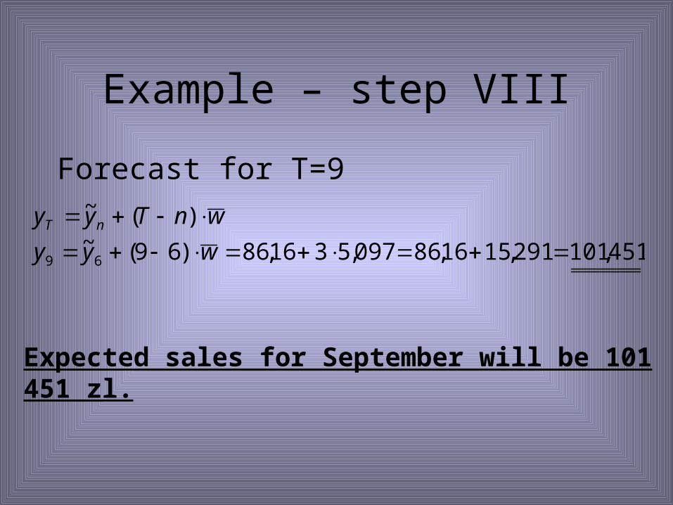
Example – step VIII
Forecast for T=9
451,101291,1516,86097,5316,86)69(~)(~
69 wyy
wnTyy nT
Expected sales for September will be 101 451 zl.