SCF methods for energies and properties of large molecular systems

Trygve Helgaker, University of Oslo, Norway

Filip Paw lowski, Simen Reine, Erik Tellgren

Stinne Høst, Branislav Jansık, Poul Jørgensen, Pekka Manninen, Jeppe Olsen,

University of Aarhus, Denmark

Sonia Coriani, University of Trieste, Italy

Pawe l Sa lek, Royal Institute of Technology, Sweden

Electron Correlation for the Whole Periodic Table

– a theoretical symposium in honour of Bjorn Roos –

International Conference of Computational Methods in Sciences and Engineering

(ICCMSE 2006)

October 27–November 1, 2006

Hotel Panorama, Chania, Crete, Greece

1

Self-consistent field (SCF) theory for large systems

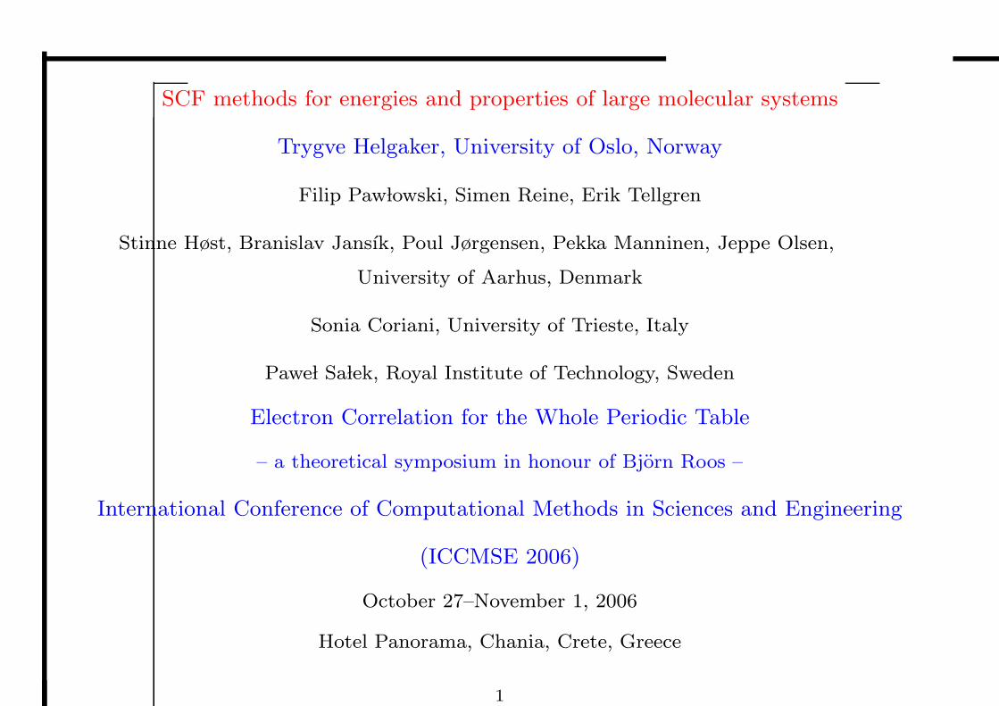
• The development of SCF methods for large systems presents several challenges:

– expensive and difficult Fock/Kohn–Sham evaluation

– expensive diagonalization and difficult SCF convergence

– DFT functionals may perform poorly for large systems

• Consider the optimization of the SCF energy (here LDA) of molecular systems:

– small systems

dominated by

KS-matrix evaluation,

with linear scaling

– large systems

dominated by SCF

diagonalization, with

cubic scaling 200 400 600 800 1000atoms

20

40

60

80

100

mins

SCF

Coulomb

LDA XC

• We shall here consider an SCF theory that avoids MOs and diagonalization

– it works directly in terms of the density matrix for energy and properties

– it involves only additions and multiplications of (sparse) one-electron matrices

– for large (sparse systems), the calculations scale linearly with system size

2

Direct optimization of the density matrix

• Consider the direct optimization of the density matrix:

E(D) = TrDh + 2-el. part

– there are constraints on the density matrix

D = DT| {z }

symmetry

, TrDS = N| {z }trace

, DSD = D| {z }idempotency

• Any other valid density matrix D(X) can then be generated from this matrix:

D(X) = exp(−XS)D exp(SX)| {z }exponential parameterization

, XT = −X| {z }antisymmetric

– Helgaker, Jørgensen and Olsen: Molecular Electronic-Structure Theory (Wiley, 2000)

– Head-Gordon and coworkers, MolPhys 101, 37 (2003), JCP 118, 6144 (2003)

• We can obtain any valid density matrix, in the AO basis, without recourse to MOs!

– in particular, we may optimize the energy by freely varying Xµν with µ > ν:

Emin(X) = minX

[TrD(X)h + 2-el. part]

• Is this use of D(X) a practical proposition?

3

Two questions about D(X) = exp(−XS)D exp(SX)

• Can it be evaluated efficiently?

– we use a generalized Baker–Campbell–Hausdorff (BCH) expansion:

D(X) = D +ˆD,X

˜S

+ 12

ˆˆD,X

˜S,X

˜S

+ · · ·

– we have here introduced the S commutatorˆD,X

˜S

= DSX−XSD

– converges rapidly (purification may be necessary), in about 10 matrix multiplications

• Are redundancies a problem?

– the AO space consists of two parts: the occupied space and the virtual space

P = DS (onto occupied space), Q = I−DS (onto virtual space)

– only rotations between the occupied and virtual spaces are nonredundant:

X = PXPT + QXQT

| {z }redundant

+ PXQT + QXPT

| {z }Xov

– to avoid problems with redundancies, we use the projected parameterization

D(X) = exp(−XovS)D exp(SXov), XT = −X

4

Diagonalization-free Roothaan–Hall SCF optimization

• The SCF (Fock or Kohn–Sham) energy may, in principle, be optimized directly:

Emin = minX

E(X) ⇔ F(D)DS = SDF(D)| {z }stationary condition

– a difficult global minimization problem!

• In MO theory, the Roothaan–Hall SCF scheme works well, especially with DIIS:

F = h + g(D)F⇄

DFC = SCǫ; Dnew = CoccC

Tocc

– each diagonalization is equivalent to minimizing the sum of the (occ.) orbital energies

ε(X) =X

I

ǫI = TrD(X)F

• By analogy with MO theory, we set up the following Roothaan–Hall SCF scheme:

F = h + g(D)F⇄

Dεmin = min

X

TrD(X)F; Dnew = D(X∗)

– at each SCF iteration, we minimize Tr D(X)F with respect to X

– the new density is then obtained by expansion of D(X) with the minimizer X∗

• We thus avoid MOs and diagonalization but retain the SCF iterations

5

Newton minimization of the Roothaan–Hall energy function

• At each SCF iteration, our task is to minimize the Roothaan–Hall energy function

ε(X) = TrD(X)F = TrDF + TrˆD,X

˜SF + 1

2Tr

ˆˆD,X

˜S,X

˜SF + · · ·

• Truncating at second order and setting the gradient to zero, we obtain the Newton step:

H−X+S− + S−X+H− = G− ← the Roothaan–Hall (RH) Newton equation

– where the (negative) gradient and Hessian matrices are given by

G = Fvo − Fov

H = Fvv − Foo F = Foo+Fov+Fvo+Fvv

• Because of their large dimensions, the Newton equations cannot be solved directly

– transformation to orthonormal Lowdin basis: A± = S±1/2AS±1/2

– S−1/2 precalculated: Z0 = I, Zn+1 = 12Zn (3I− λZnSZn) for ‖I− λS‖2 < 1

– solution by the preconditioned conjugate-gradient method (typically 10 iterations)

– elementary (sparse) matrix manipulations (typically less than 100 multiplications)

• A RH diagonalization corresponds to an exact minimization (many Newton steps)

– however, a partial minimization will do (one RH Newton step is sufficient)

6

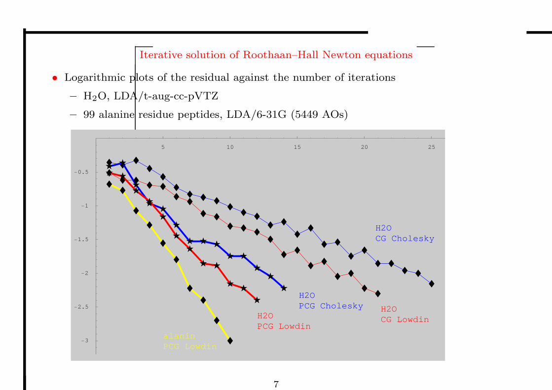
Iterative solution of Roothaan–Hall Newton equations

• Logarithmic plots of the residual against the number of iterations

– H2O, LDA/t-aug-cc-pVTZ

– 99 alanine residue peptides, LDA/6-31G (5449 AOs)

5 10 15 20 25

-3

-2.5

-2

-1.5

-1

-0.5

H2OPCG Lowdin

H2OPCG Cholesky H2O

CG Lowdin

H2OCG Cholesky

alaninPCG Lowdin

7

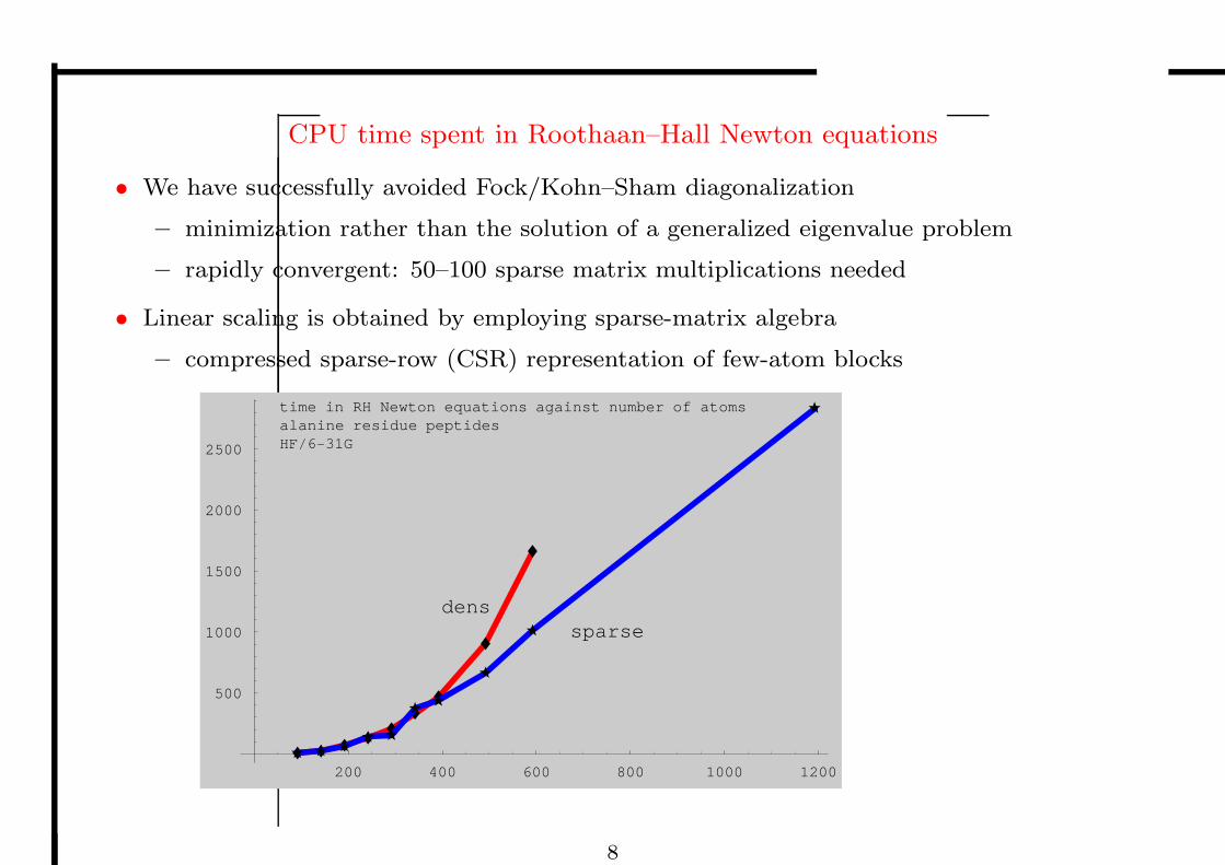
CPU time spent in Roothaan–Hall Newton equations

• We have successfully avoided Fock/Kohn–Sham diagonalization

– minimization rather than the solution of a generalized eigenvalue problem

– rapidly convergent: 50–100 sparse matrix multiplications needed

• Linear scaling is obtained by employing sparse-matrix algebra

– compressed sparse-row (CSR) representation of few-atom blocks

200 400 600 800 1000 1200

500

1000

1500

2000

2500

time in RH Newton equations against number of atomsalanine residue peptidesHF�6-31G

sparsedens

8

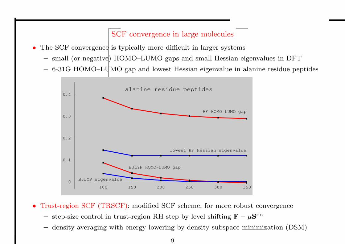
SCF convergence in large molecules

• The SCF convergence is typically more difficult in larger systems

– small (or negative) HOMO–LUMO gaps and small Hessian eigenvalues in DFT

– 6-31G HOMO–LUMO gap and lowest Hessian eigenvalue in alanine residue peptides

100 150 200 250 300 3500

0.1

0.2

0.3

0.4alanine residue peptides

HF HOMO-LUMO gap

B3LYP HOMO-LUMO gap

lowest HF Hessian eigenvalue

B3LYP eigenvalue

• Trust-region SCF (TRSCF): modified SCF scheme, for more robust convergence

– step-size control in trust-region RH step by level shifting F− µSoo

– density averaging with energy lowering by density-subspace minimization (DSM)

9

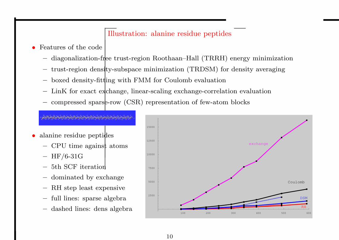
Illustration: alanine residue peptides

• Features of the code

– diagonalization-free trust-region Roothaan–Hall (TRRH) energy minimization

– trust-region density-subspace minimization (TRDSM) for density averaging

– boxed density-fitting with FMM for Coulomb evaluation

– LinK for exact exchange, linear-scaling exchange-correlation evaluation

– compressed sparse-row (CSR) representation of few-atom blocks

• alanine residue peptides

– CPU time against atoms

– HF/6-31G

– 5th SCF iteration

– dominated by exchange

– RH step least expensive

– full lines: sparse algebra

– dashed lines: dens algebra100 200 300 400 500 600

2500

5000

7500

10000

12500

15000

exchange

Coulomb

DSM

RH

10

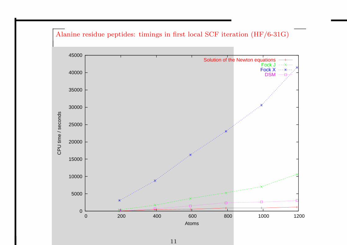
Alanine residue peptides: timings in first local SCF iteration (HF/6-31G)

0

5000

10000

15000

20000

25000

30000

35000

40000

45000

0 200 400 600 800 1000 1200

CP

U ti

me

/ sec

onds

Atoms

Solution of the Newton equationsFock JFock X

DSM

11

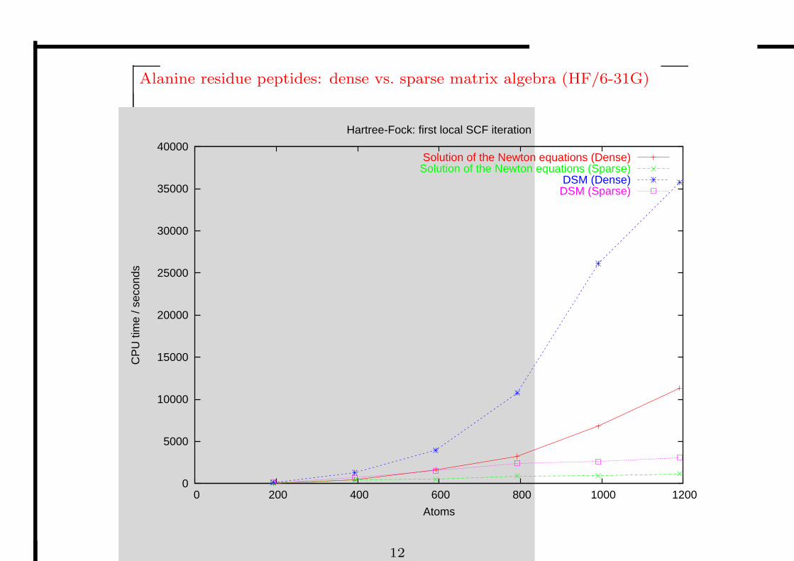
Alanine residue peptides: dense vs. sparse matrix algebra (HF/6-31G)

0

5000

10000

15000

20000

25000

30000

35000

40000

0 200 400 600 800 1000 1200

CP

U ti

me

/ sec

onds

Atoms

Hartree-Fock: first local SCF iteration

Solution of the Newton equations (Dense)Solution of the Newton equations (Sparse)

DSM (Dense)DSM (Sparse)

12

Response theory

• The expectation value of A in the presence of a perturbation Vω of frequency ω:

˙t˛A

˛t¸

=˙0

˛A

˛0

¸+

Z〈〈A; Vω〉〉ω exp (−iωt) dω + · · ·

– the linear-response function 〈〈A; Vω〉〉ω carries information about the first-order

change in the expectation value

• The linear-response function may be represented compactly as:

〈〈A; V ω〉〉ω = −A[1]T`E[2] − ωS[2]

´−1V

[1]ω| {z }

linear equations

←

8><>:

E[2] electronic Hessian

S[2] metric matrix

A[1] = vec

`

ADS − SDA´

• In practice, the response functions are evaluated by solving a set of linear equations`E[2] − ωS[2]

´N[1] = −V

[1]ω

〈〈A; V ω〉〉ω = A[1]TN[1]

• Excitation energies as poles of linear response function (RPA):`E[2] − ωS[2]

´X = 0

• Can these tasks be accomplished efficiently in the AO basis?

13

Solution of the response equations

• The response equations are solved in the same manner as the RH Newton equations:`E[2] − ωS[2]

´x = V[1]

– generation of an iterative subspace until the residual is sufficiently small

R =`E[2] − ωS[2]

´x−V[1]

• Key step: multiplication of Hessian and metric matrices with trial vectors (matrices)

E[2](X) = (Fvv − Foo)XS + SX(Fvv − Foo) + gvo([D,X]S)− gov([D,X]S)

S[2](X) = SooXSvv − SvvXSoo

– requires recalculation of Fock/Kohn–Sham matrix with modified AO density matrix

– trial matrices always added in pairs X and XT

• For rapid convergence, the residual vector is preconditioned

eR = M−1R, M = E[2] − ωS[2] (but without red part!)

– transformation to orthogonal basis (Cholesky or Lowdin)

– nondiagonal preconditioning requires typically 7 conjugate-gradient steps

• With this preconditioner, the response equations converge in 5–10 iterations

– indeed, this is the same convergence as in the canonical MO basis

14

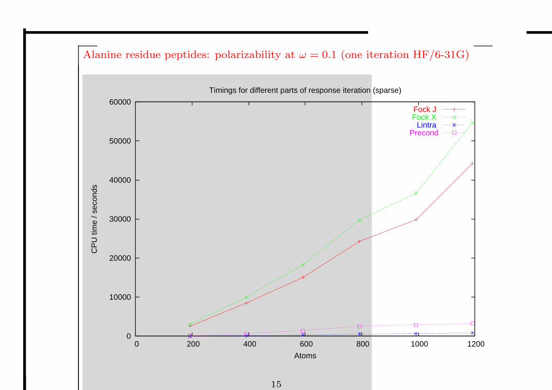
Alanine residue peptides: polarizability at ω = 0.1 (one iteration HF/6-31G)

0

10000

20000

30000

40000

50000

60000

0 200 400 600 800 1000 1200

CP

U ti

me

/ sec

onds

Atoms

Timings for different parts of response iteration (sparse)

Fock J Fock X

Lintra Precond

15

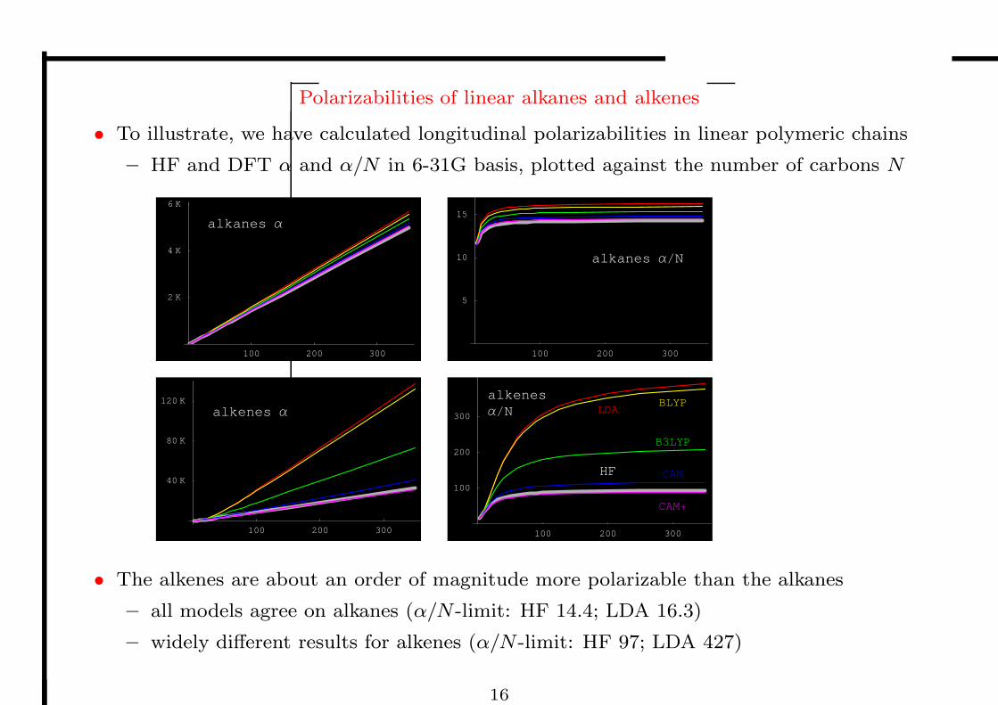
Polarizabilities of linear alkanes and alkenes

• To illustrate, we have calculated longitudinal polarizabilities in linear polymeric chains

– HF and DFT α and α/N in 6-31G basis, plotted against the number of carbons N

100 200 300

40 K

80 K

120 Kalkenes Α

100 200 300

100

200

300LDA

BLYP

B3LYP

CAMHF

CAM+

alkenesΑ�N

100 200 300

2 K

4 K

6 K

alkanes Α

100 200 300

5

10

15

alkanes Α�N

• The alkenes are about an order of magnitude more polarizable than the alkanes

– all models agree on alkanes (α/N -limit: HF 14.4; LDA 16.3)

– widely different results for alkenes (α/N -limit: HF 97; LDA 427)

16

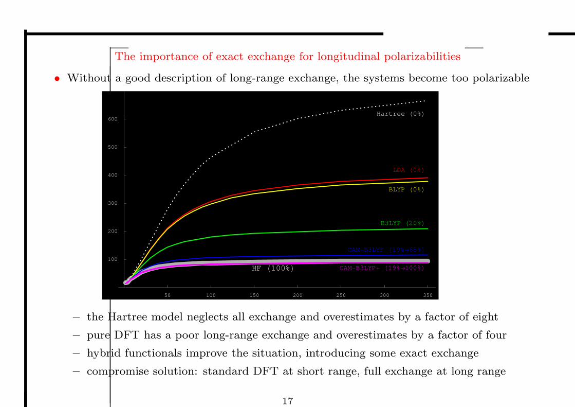
The importance of exact exchange for longitudinal polarizabilities

• Without a good description of long-range exchange, the systems become too polarizable

50 100 150 200 250 300 350

100

200

300

400

500

600

LDA H0%L

BLYP H0%L

B3LYP H20%L

CAM-B3LYP H19%®65%L

HF H100%L CAM-B3LYP+ H19%®100%L

Hartree H0%L

– the Hartree model neglects all exchange and overestimates by a factor of eight

– pure DFT has a poor long-range exchange and overestimates by a factor of four

– hybrid functionals improve the situation, introducing some exact exchange

– compromise solution: standard DFT at short range, full exchange at long range

17

Asymptotic behaviour of group polarizabilities

• How does the group polarizability converge towards the infinite limit?

α∞ − αN = eN−1 +O(N−2) Kudin et al., JCP 122, 134907 (2005)

– this behaviour is universal, holding at all levels of theory

• Log–log plots of α∞ − αN for alkanes and alkenes:

2 10 60 350

0.1

1

10

2 10 60 3501

10

100

– limit obtained by extrapolation α∞ = (αN − αM )/(N −M)

– straight lines of slope −1 superimposed through the points at N = 350

• The asymptotic region is reached with C30H62 (alkanes) and C60H62 (alkenes)

– alkane α∞ predicted to within 1% from C30H62

– alkene α∞ predicted to within 1% from C60H62 for HF and from C150H152 for LDA

18

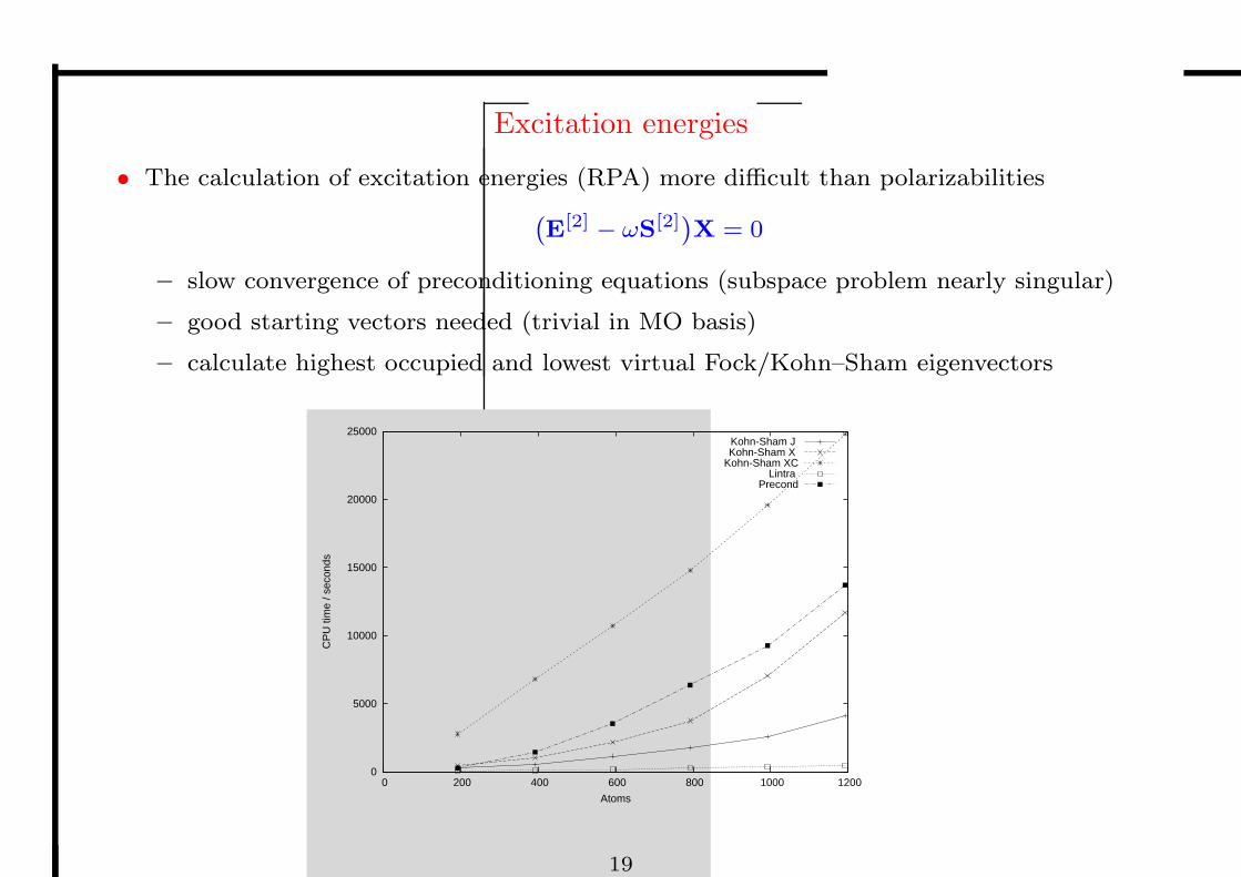
Excitation energies

• The calculation of excitation energies (RPA) more difficult than polarizabilities

`E[2] − ωS[2]

´X = 0

– slow convergence of preconditioning equations (subspace problem nearly singular)

– good starting vectors needed (trivial in MO basis)

– calculate highest occupied and lowest virtual Fock/Kohn–Sham eigenvectors

0

5000

10000

15000

20000

25000

0 200 400 600 800 1000 1200

CP

U ti

me

/ sec

onds

Atoms

Kohn-Sham J Kohn-Sham X

Kohn-Sham XCLintra

Precond

19

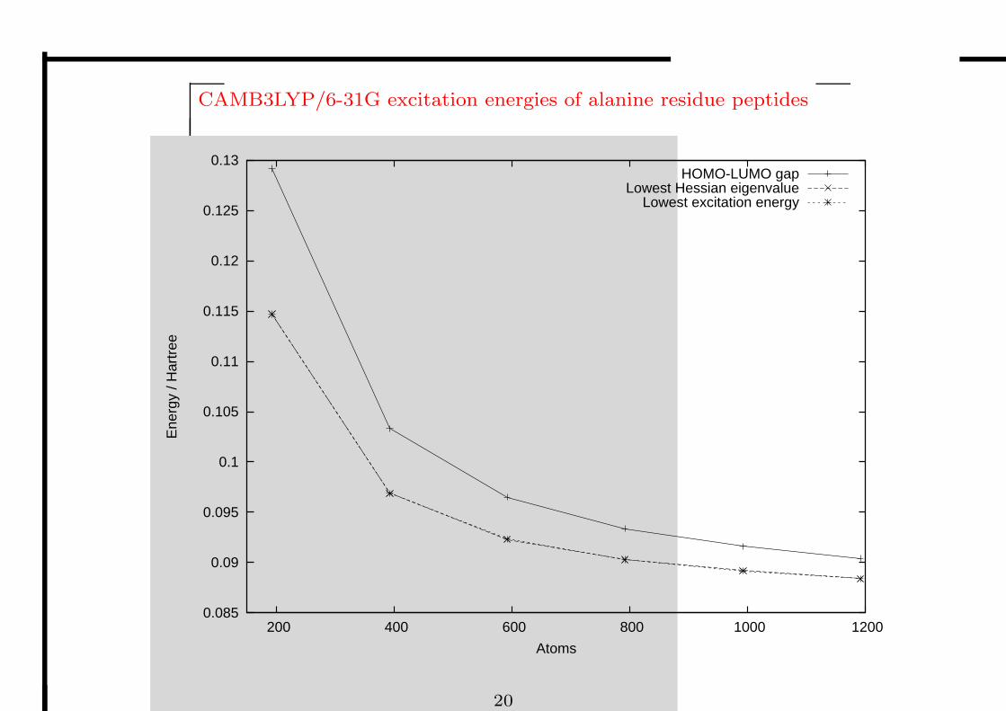
CAMB3LYP/6-31G excitation energies of alanine residue peptides

0.085

0.09

0.095

0.1

0.105

0.11

0.115

0.12

0.125

0.13

200 400 600 800 1000 1200

Ene

rgy

/ Har

tree

Atoms

HOMO-LUMO gapLowest Hessian eigenvalue

Lowest excitation energy

20

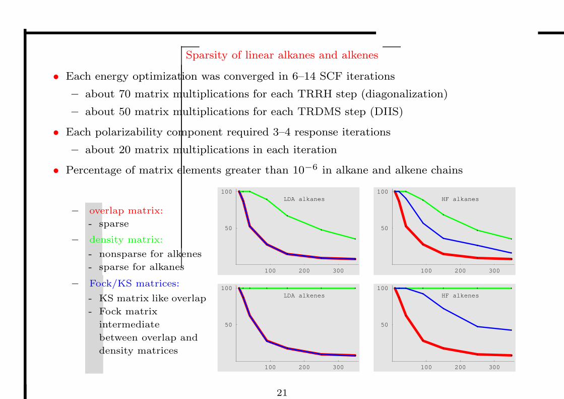
Sparsity of linear alkanes and alkenes

• Each energy optimization was converged in 6–14 SCF iterations

– about 70 matrix multiplications for each TRRH step (diagonalization)

– about 50 matrix multiplications for each TRDMS step (DIIS)

• Each polarizability component required 3–4 response iterations

– about 20 matrix multiplications in each iteration

• Percentage of matrix elements greater than 10−6 in alkane and alkene chains

– overlap matrix:

- sparse

– density matrix:

- nonsparse for alkenes

- sparse for alkanes

– Fock/KS matrices:

- KS matrix like overlap

- Fock matrix

intermediate

between overlap and

density matrices

100 200 300

50

100LDA alkenes

100 200 300

50

100HF alkenes

100 200 300

50

100LDA alkanes

100 200 300

50

100HF alkanes

21

Conclusions

• We have discussed the optimization of SCF energies without orbital generation

– direct optimization of density matrix in the AO basis

– in each SCF iteration, we replace diagonalization by minimization

– one Newton step is usually enough

– 50–100 matrix multiplications typically required

– linear scaling achieved with sparse matrix algebra

• Large molecules represent a more difficult minimization problem

– small Hessian eigenvalues for pure DFT

– trust-region SCF: careful step-size control

– revert to second-order if necessary

• Linear-response calculations are straightforward in the AO basis

– one Fock/Kohn–Sham matrix build and 20 matrix multiplications pr. iteration

– stable convergence in 5–10 iterations

– preconditioning requires typically 7 iterations

• The calculation of excitation energies more difficult

– near singular subspace problem for preconditioning

– good starting vectors needed

22