Long wave modeling. - Boussinesq equations; motivation and...

Long wave modeling.

Boussinesq equations; motivation and derivationMEK4320

Geir Pedersen

Department of Mathematics, UiO

December 5, 2014

Geir Pedersen Boussinesq

Primitive and general hydrodynamicequations


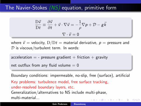
The Navier-Stokes (NS) equation, primitive form

D~v

Dt≡

∂~v

∂t+ ~v · ∇~v = −

1

ρ∇p +D − g~k

∇ · ~v = 0

where ~v = velocity, D/Dt = material derivative, p = pressure andD is viscous/turbulent term. In words:

acceleration = - pressure gradient + friction + gravity

net outflux from any fluid volume = 0

Boundary conditions: impermeable, no-slip, free (surface), artificial

Key problems: turbulence model, free surface tracking,under-resolved boundary layers, etc.Generalization/alternatives to NS include multi-phase,multi-material...


Applicability of primitive models

General, but inaccurate, free surface techniques (VOF, SPH...)

Industrial (CFX, Fluent...) and open-source (OpenFoam)solvers

Computations readily become very heavy ⇒ numericalsolutions are under-resolved or unattainable

Thin wall boundary layers; cannot be resolved

Feasible only in local and idealized studies

The burden of the computations often lead to wavering of thephysics ?

Analytic solutions are sparse, circumstantial and cumbersome

Surprisingly (?) little insight in hydrodynamic wave theory yetstem from “full computational models”.

Simplified theories are still crucial, but general models

become increasingly important


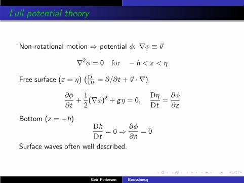
Full potential theory

Non-rotational motion ⇒ potential φ: ∇φ ≡ ~v

∇2φ = 0 for − h < z < η

Free surface (z = η) (DDt

= ∂/∂t + ~v · ∇)

∂φ

∂t+

1

2(∇φ)2 + gη = 0,

Dη

Dt=

∂φ

∂z

Bottom (z = −h)Dh

Dt= 0 ⇒

∂φ

∂n= 0

Surface waves often well described.


Potential flow models

1 Integral equation discretized by panels. Boundary locationupdated in time as part of the method.

2 FFT techniques; approximations at free surface

Not incorporable: viscous effects, turbulence, overturning waves,Coriolis force...Computation still heavy. Useful for local simulations and forassessing validity of simpler models.More efficient and robust models must be employed for large scalemodeling


Approximative theories


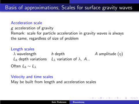
Basis of approximations; Scales for surface gravity waves

Acceleration scaleg acceleration of gravityRemark: scale for particle acceleration in gravity waves is alwaysthe same, regardless of size of problem

Length scalesλ wavelength h depth A amplitude (η)Lh depth variations Lλ variation of λ, A...

Often Lh ∼ Lλ

Velocity and time scalesMay be built from length and acceleration scales


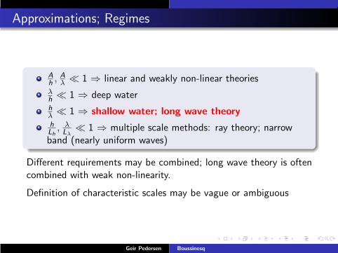
Approximations; Regimes

Ah, Aλ≪ 1 ⇒ linear and weakly non-linear theories

λh≪ 1 ⇒ deep water

hλ≪ 1 ⇒ shallow water; long wave theory

hLh, λLλ

≪ 1 ⇒ multiple scale methods: ray theory; narrowband (nearly uniform waves)

Different requirements may be combined; long wave theory is oftencombined with weak non-linearity.

Definition of characteristic scales may be vague or ambiguous


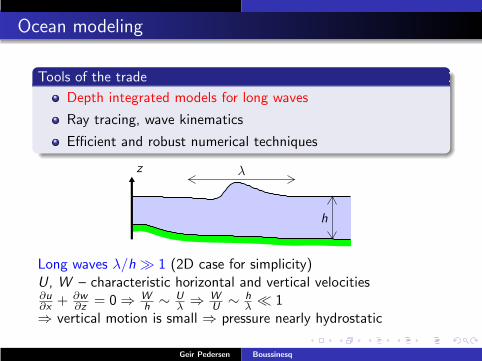
Ocean modeling

Tools of the trade

Depth integrated models for long waves

Ray tracing, wave kinematics

Efficient and robust numerical techniques

z λ

h

Long waves λ/h ≫ 1 (2D case for simplicity)U, W – characteristic horizontal and vertical velocities∂u∂x

+ ∂w∂z

= 0 ⇒ Wh

∼ Uλ⇒ W

U∼ h

λ≪ 1

⇒ vertical motion is small ⇒ pressure nearly hydrostatic


Nonlinear Shallow Water Equations

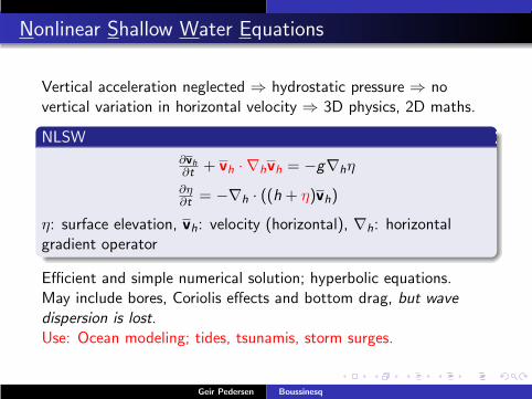
Vertical acceleration neglected ⇒ hydrostatic pressure ⇒ novertical variation in horizontal velocity ⇒ 3D physics, 2D maths.

NLSW

∂vh∂t

+ vh · ∇hvh = −g∇hη

∂η∂t

= −∇h · ((h + η)vh)

η: surface elevation, vh: velocity (horizontal), ∇h: horizontalgradient operator

Efficient and simple numerical solution; hyperbolic equations.May include bores, Coriolis effects and bottom drag, but wavedispersion is lost.Use: Ocean modeling; tides, tsunamis, storm surges.


Dispersive long wave models

Models developed by perturbation/iteration/series expansion,assuming smallǫ ≡ (H/λ)2 and α ≡ A/H, where H is typical depth.Leading pressure modifications by vertical accelerations included.Huge diversity in in formulations and accuracy

Boussinesq type models

1880→ Theoretical applications (KdV...)

1966 first numerical Boussinesq models put to use

1990→ new formulations, increased validity range

Increase of computer power ⇒ large scale models feasible

Important for some tsunami features

Important model for coastal engineering

A step toward more general models from (N)LSW;assessment of dispersion effects


Derivation of Boussinesq equations


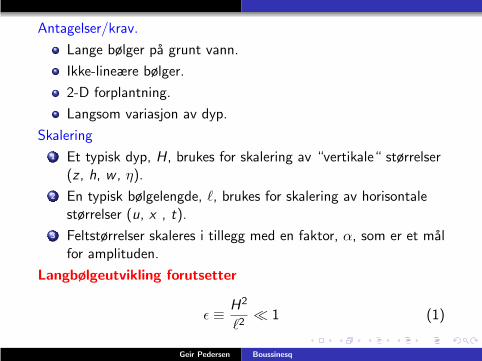
Antagelser/krav.

Lange bølger pa grunt vann.

Ikke-lineære bølger.

2-D forplantning.

Langsom variasjon av dyp.

Skalering

1 Et typisk dyp, H, brukes for skalering av “vertikale“ størrelser(z , h, w , η).

2 En typisk bølgelengde, ℓ, brukes for skalering av horisontalestørrelser (u, x , t).

3 Feltstørrelser skaleres i tillegg med en faktor, α, som er et malfor amplituden.

Langbølgeutvikling forutsetter

ǫ ≡H2

ℓ2≪ 1 (1)


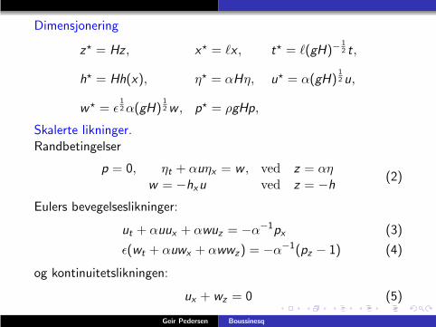
Dimensjonering

z⋆ = Hz , x⋆ = ℓx , t⋆ = ℓ(gH)−12 t,

h⋆ = Hh(x), η⋆ = αHη, u⋆ = α(gH)12 u,

w⋆ = ǫ12α(gH)

12w , p⋆ = ρgHp,

Skalerte likninger.Randbetingelser

p = 0, ηt + αuηx = w , ved z = αηw = −hxu ved z = −h

(2)

Eulers bevegelseslikninger:

ut + αuux + αwuz = −α−1px (3)

ǫ(wt + αuwx + αwwz) = −α−1(pz − 1) (4)

og kontinuitetslikningen:

ux + wz = 0 (5)


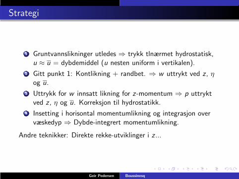
Strategi

1 Gruntvannslikninger utledes ⇒ trykk tlnærmet hydrostatisk,u ≈ u = dybdemiddel (u nesten uniform i vertikalen).

2 Gitt punkt 1: Kontlikning + randbet. ⇒ w uttrykt ved z , ηog u.

3 Uttrykk for w innsatt likning for z-momentum ⇒ p uttryktved z , η og u. Korreksjon til hydrostatikk.

4 Insetting i horisontal momentumlikning og integrasjon overvæskedyp ⇒ Dybde-integrert momentumlikning.

Andre teknikker: Direkte rekke-utviklinger i z ...


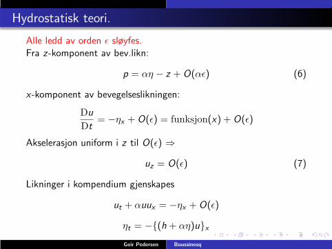
Hydrostatisk teori.

Alle ledd av orden ǫ sløyfes.Fra z-komponent av bev.likn:

p = αη − z + O(αǫ) (6)

x-komponent av bevegelseslikningen:

Du

Dt= −ηx + O(ǫ) = funksjon(x) + O(ǫ)

Akselerasjon uniform i z til O(ǫ) ⇒

uz = O(ǫ) (7)

Likninger i kompendium gjenskapes

ut + αuux = −ηx + O(ǫ)

ηt = −{(h + αη)u}x


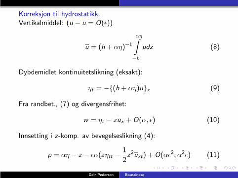
Korreksjon til hydrostatikk.Vertikalmiddel: (u − u = O(ǫ))

u = (h + αη)−1

αη∫

−h

udz (8)

Dybdemidlet kontinuitetslikning (eksakt):

ηt = −{(h + αη)u}x (9)

Fra randbet., (7) og divergensfrihet:

w = ηt − zux + O(α, ǫ) (10)

Innsetting i z-komp. av bevegelseslikning (4):

p = αη − z − ǫα(zηtt −1

2z2uxt) + O(αǫ2, α2ǫ) (11)


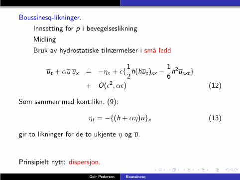
Boussinesq-likninger.

Innsetting for p i bevegelseslikning

Midling

Bruk av hydrostatiske tilnærmelser i sma ledd

ut + αu ux = −ηx + ǫ{1

2h(hut)xx −

1

6h2uxxt}

+ O(ǫ2, αǫ) (12)

Som sammen med kont.likn. (9):

ηt = −{(h + αη)u}x (13)

gir to likninger for de to ukjente η og u.

Prinsipielt nytt: dispersjon.


More on Boussinesq type equations


Depth integrated theory; Boussinesq

Boussinesq equations with 2 horizontal dimensions

∂vh∂t

+ αvh · ∇hvh = −∇hη + ǫ(

12h∇h∇h · (h

∂vh∂t

)− 16h2∇h∇h ·

∂vh∂t

)

−ǫκh2(∇3hη +∇h∇h ·

∂vh∂t

)+O(ǫ2, αǫ)

∂η∂t

= −∇h · ((h + αη)vh)

Derivation as with 1 horizontal dimension.Blue term =O(ǫ2, ǫα): optimization of dispersion propertiesNumerical solution much heavier than for shallow water eq. –implicit solution strategy needed. Still, much faster to solv thanprimitive equations. Wave dispersion included.


The zα formulation

Popular formulation from Nwogu, later extended by others(Kennedy, Kirby, Wu, Liu, Lynett..)Velocity profile

~v = ~vs + ǫ(zα∇h

∂η

∂t−

1

2z2α∇h∇h · ~v∗) + O(ǫ2),

~vs = surface velocity, ~v∗ velocity at any depth.Velocity at zα(x , y)v(x , y , t) ≡ ~v(x , y , zα(x , y), t),used as unknown. Optimization of disperson on flat bottom ⇒zα = −0.531hExtra nonlinearities, O(ǫα), may be kept in derivation.

zα not related to nonlinear parameter α


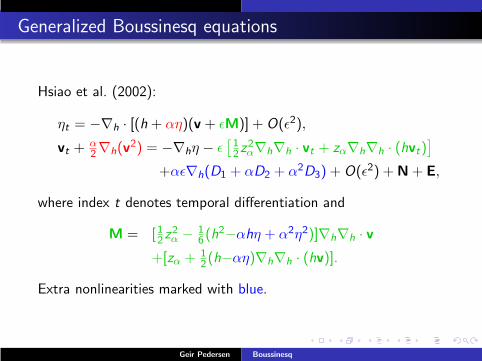
Generalized Boussinesq equations

Hsiao et al. (2002):

ηt = −∇h · [(h + αη)(v + ǫM)] + O(ǫ2),

vt +α2∇h(v

2) = −∇hη − ǫ[

12z2α∇h∇h · vt + zα∇h∇h · (hvt)

]

+αǫ∇h(D1 + αD2 + α2D3) + O(ǫ2) +N+ E,

where index t denotes temporal differentiation and

M = [12z2α − 1

6(h2−αhη + α2η2)]∇h∇h · v

+[zα + 12(h−αη)∇h∇h · (hv)].

Extra nonlinearities marked with blue.


Furthermore...

D1 = η∇ · (hvt)−12z2αv · ∇∇v − zαv · ∇∇ · (hv)− 1

2(∇ · (hv))2,

D2 =12η2∇ · vt + ηv∇∇ · (hv)− η∇ · (hv)∇ · v,

D3 =12η2

[

v · ∇∇ · v − (∇ · v)2]

,

E = H−1∇h(ν(x , y , t)∇h(Hv),

N = −αµKH|v|v.

Unsystematic terms:E is dissipation term for capturing of breaking wavesN is bottom drag.Programs freely available on WEB (Funwave and Coulwave).There are issues with these equations


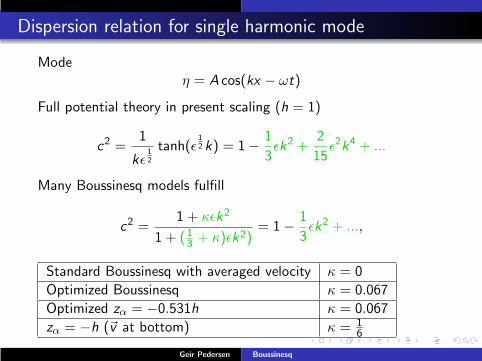
Dispersion relation for single harmonic mode

Modeη = A cos(kx − ωt)

Full potential theory in present scaling (h = 1)

c2 =1

kǫ12

tanh(ǫ12 k) = 1−

1

3ǫk2 +

2

15ǫ2k4 + ...

Many Boussinesq models fulfill

c2 =1 + κǫk2

1 + (13+ κ)ǫk2)

= 1−1

3ǫk2 + ...,

Standard Boussinesq with averaged velocity κ = 0

Optimized Boussinesq κ = 0.067

Optimized zα = −0.531h κ = 0.067

zα = −h (~v at bottom) κ = 16


Dispersion properties

Exact

κ = 0

κ = 0.067

κ = 16

KdV

λ/h

cg

κ = 16→ u at bottom, κ = 0 → averaged u,

κ = 0.067 → optimal choicecg = dω/dk – group velocity


Effect of dispersion

full pot stand B.

opt B.

x

η

Evolution from short initial elevationBlack: half the initial condition, width ∼ 3 depthsFront: Good agreement for all Boussinesq formulationsRear: Improved model superior, standard B. too dispersive

Observe: No corresponding improvement for steep bottomgradients


Utledning av KdV likninger.


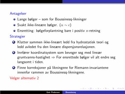
Antagelser

Lange bølger – som for Boussinesq-likninger

Svakt ikke-lineære bølger. (α ∼ ǫ)

Ensretting: bølgeforplantning bare i positiv x-retning

Strategier

1 Klatter sammen ikke-lineært ledd fra hydrostatisk teori ogledd avledet fra den lineære dispersjonsrelasjonen.

2 Innfører koordinatsystem som beveger seg med lineærgruntvanns-hastighet ⇒ For ensrettede bølger vil alt endre seglangsomt i tiden.

3 Finne korreksjoner pa likningene for Riemann-invarianteneinnenfor rammen av Boussinesq-likningene.

Velger alternativ 2


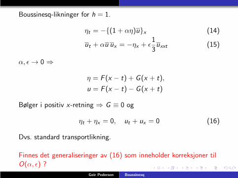
Boussinesq-likninger for h = 1.

ηt = −{(1 + αη)u}x (14)

ut + αu ux = −ηx + ǫ1

3uxxt (15)

α, ǫ → 0 ⇒

η = F (x − t) + G (x + t),

u = F (x − t)− G (x + t)

Bølger i positiv x-retning ⇒ G ≡ 0 og

ηt + ηx = 0, ut + ux = 0 (16)

Dvs. standard transportlikning.

Finnes det generaliseringer av (16) som inneholder korreksjoner tilO(α, ǫ) ?


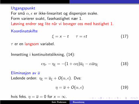
UtgangspunktFor sma α, ǫ er ikke-linearitet og dispersjon svake.Form varierer svakt, fasehastighet nær 1.Løsning endrer seg lite nar vi beveger oss med hastighet 1.

Koordinatskifteξ = x − t τ = ǫt (17)

τ er en langsom variabel.

Innsetting i kontinuitetslikning, (14):

ǫητ − ηξ = −(1 + αη)uξ − αuηξ (18)

Eliminasjon av u

Ledende orden: ηξ = uξ + O(α, ǫ). Dvs:

η = u + O(α, ǫ) (19)

hvis feks. η = u = 0 for x = ∞.Geir Pedersen Boussinesq

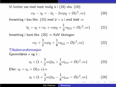
Vi kvitter oss med mest mulig u i (18) vha. (19):

ǫητ − ηξ = −uξ − 2αηηξ + O(ǫ2, αǫ) (20)

Innsetting i bev.likn. (15) med u = η i sma ledd ⇒

uξ = ηξ + ǫητ + αηηξ +1

3ǫηξξξ + O(ǫ2, αǫ) (21)

Innsetting i kont.likn. (20) ⇒ KdV likningen:

ǫητ +3

2αηηξ +

1

6ǫηξξξ = O(ǫ2, αǫ) (22)

TilbaketransformasjonGjeninnføres x og t :

ηt + (1 +3

2αη)ηx +

1

6ǫηxxx = O(ǫ2, αǫ) (23)

Eller; ηt = ηx + O(α, ǫ)⇒

ηt + (1 +3

2αη)ηx −

1

6ǫηxxt = O(ǫ2, αǫ) (24)


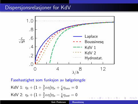
Dispersjonsrelasjoner for KdV

Laplace

Boussinesq

KdV 1

KdV 2Hydrostat.

λ/h

c√gh

Fasehastighet som funksjon av bølgelengde

KdV 1: ηt + (1 + 32αη)ηx +

ǫ6ηxxx = 0

KdV 2: ηt + (1 + 32αη)ηx −

ǫ6ηxxt = 0


What is gained by long wave theory

1 Physical contents more transparent

2 Important closed form solutions of NLSW and the KdVequations

3 NLSW equations are hyperbolic with characteristics andshocks

4 Unknown upper bound of fluid replaced by coefficients in η

5 The number of dimensions reduced by 1 (depth integration)

Last two points crucial for numerical solution


Long wave modeling. - Boussinesq equations; motivation and...

Documents

Transcript of Long wave modeling. - Boussinesq equations; motivation and...