Faculties of Engineering, Science, and Medicine - Aalborg Universitet
105
τ y y y τ y y τ y · -7 2 · -7 · -6 2 · -11 · -9 2
Transcript of Faculties of Engineering, Science, and Medicine - Aalborg Universitet
Faculties of Engineering, Science, and MedicineAalborg University
Department of Biotechnology, Chemistry, and Environmental Engineering
TITLE:Comparison of Shear andCompressive Yield StressRatio for Sewage Sludgeand Inorganic ParticulateSuspensions
PROJECT PERIOD:September 1st 2007 -June 6th 2008
PROJECT GROUP:K9-10K
AUTHOR:Maria Kristjansson
SUPERVISORS:Kristian KeidingPeter J. Scales
NUMBER OF COPIES: 4
REPORT PAGES: 78
TOTAL PAGES: 95
ENCLOSED: CD-rom
SYNOPSIS:
The shear (τy) and compressive (Py) yield stress behaviourof a coagulated alumina suspension, a sewage sludge, anda dual-polymer occulated alumina suspension were char-acterised with focus on determining the variation in thePy/τy ratio with solids volume fraction. Shear yield stresswas determined using the vane technique developed byNguyen and Boger (1983) by employing dierent vane di-mensions. Shear yield stress values ranging from 0.9-15,000Pa were measured. Compressive yield stress was deter-mined through equilibrium pressure ltration, centrifuga-tion, and batch settling tests. Compressive yield stressescould be determined in the range from 0.007-300 kPa.Sewage sludge is dicult to characterise due to its slowdewatering properties. A occulated alumina suspension,expected to exhibit sludge behaviour, was produced as apotential substitute.The three suspensions were more easily deformed by shearthan by compression. The Py/τy ratios increased with vol-ume fraction for all three suspensions. An increase from2-14 was observed for the coagulated alumina suspension inthe volume fraction range from 0.075-0.50 v/v. The ratioof sewage sludge increased from 5-8 in the volume fractionrange from 0.035-0.09 v/v and the ratio of the occulatedalumina suspension increased from 8-11 in the volume frac-tion range from 0.09-0.43 v/v.The ltration behaviour of the coagulated alumina sus-pension was traditional and the solids diusivity con-stant at 1·10−7 m2/s with volume fraction above the gelpoint. The occulated alumina suspension exhibited non-traditional ltration behaviour (a behaviour often exhibitedby sludges) at low pressures, 5-20 kPa, and a non classi-ed ltration behaviour at higher pressures, 40-300 kPa.The solids diusivity ranged from 1·10−7-2·10−6 m2/s andshowed a maximum near the gel point and the decrease withvolume fraction was followed by an increase. The sewagesludge showed a similar solids diusivity with volume frac-tion which varied from 6·10−11-5·10−9 m2/s.

II
De Ingeniør-, Natur- og Sundhedsvidenskabelige FakulteterAalborg Universitet
Institut for Kemi, Miljøteknik og Bioteknologi
TITEL:Sammenligning af kom-pressiblet and shear yieldstress for kloak slam oguorganiske partikulæresuspensioner
PROJEKTPERIODE:1. september 2007 -6. juni 2008
PROJEKTGRUPPE:K9-10K
FORFATTER:Maria Kristjansson
VEJLEDERE:Kristian KeidingPeter J. Scales
ANTAL KOPIER: 4
RAPPORT SIDEANTAL:78
TOTAL SIDEANTAL: 95
VEDLAGT: CD-rom
SYNOPSIS:
Variationen i kompressibel (Py) og shear (τy) yield stressaf en koaguleret aluminiumoxidsuspension, kloakslam ogen dobbelt-polymer okkuleret aluminiumoxidsuspensioner blevet undersøgt, med henblik på at bestemme variatio-nen i Py/τy forholdet, som funktion af tørstofvolumenfrak-tionen. τy blev bestemt med vane teknik metoden udvikletaf Nguyen and Boger (1983) ved at benytte forskellige vanestørrelser. τy værdier fra 0,9-15.000 Pa blev målt. Py blevbestemt ved hjælp af ligevægt trykltrering, centrifugering,og settling. Py værdier fra 0,007-300 kPa blev målt.Kloakslam er svært at karakterisere, fordi det er langsomttil at afvande. En okkuleret suspension, som forventedesat opføre sig som slam, blev fremstillet som en mulig er-statning til karakterisering af slam.De tre suspensioner blev lettere deformeret ved hjælp enshear kraft end en kompressibel kraft. Py/τy forholdetsteg som en funktion af volumenfraktionen for alle tresuspensioner. En stigning fra 2-14 blev bestemt for denkoagulerede aluminiumoxidsuspension i volumenfraktion-sområdet fra 0,075-0,50 v/v. Forholdet for kloakslam stegfra 5-8 i volumenfraktionsområdet fra 0,035-0,09 v/v ogforholdet for den okkuleret aluminiumoxidsuspension stegfra 8-11 i volumenfraktionsområdet fra 0,09-0,43 v/v.Filtrering, af den koagulerede aluminiumoxidsuspension,var traditionel, og tørstofsdiusiviteten var konstant på1·10−7 m2/s, som en funktion af volumenfraktionen overgelpunktet. Den okkulerede aluminiumoxidsuspension ud-viste en non-traditional ltrering (en ltrering ofte ob-serveret i forbindelse med ltrering af slam) ved lave tryk,5-20 kPa, og en uklassiceret ltrering ved højere tryk, 40-300 kPa. Tørstofsdiusiviteten varierede fra 1·10−7-2·10−6
m2/s, og havde et maksimum tæt på gelpunktet, hvilketblev efterfulgt af et fald for derefter at stige igen. Tørstofd-iusiviteten for kloakslam havde et lignende forløb, somfunktion af volumenfraktionen, og varierende fra 6·10−11-5·10−9 m2/s.

II
Preface
The references are stated in accordance with the Harvard Method [author, year]. If no authoris stated the publisher is given. The report is divided into chapters, sections, and subsections.The chapters are numbered with one number and its sections are numbered with an additionalnumber. Figures, tables, and equations are consecutive numbered according to the chapters.In Appendices the theoretical background of the employed methods are enclosed. Furthermorecalculation methods are found in Enclosures. Additionally experimental data can be found onthe enclosed CD-rom.
The author would like to thank Shane P. Usher and Ross G. De Kretser, The solid-liquid separa-tion group University of Melbourne, for supervision and the remaining people in the solid-liquidseparation group for help with practically matters.
..............................................................Maria Kristjansson
III

IV
Contents
1 Introduction 11.1 Problem Statement . . . . . . . . . . . . . . . . . . . . . . . . . . . . . . . . . . . 2
2 Microstructure of Suspensions 52.1 Forces Acting on Particles in a Suspension . . . . . . . . . . . . . . . . . . . . . . 5
2.2 The Electrical Double Layer . . . . . . . . . . . . . . . . . . . . . . . . . . . . . . 7
2.3 DLVO theory . . . . . . . . . . . . . . . . . . . . . . . . . . . . . . . . . . . . . . 8
2.4 Non-DLVO Forces . . . . . . . . . . . . . . . . . . . . . . . . . . . . . . . . . . . 10
3 Rheology of Suspensions 113.1 Denition of Viscoelastic Behaviour . . . . . . . . . . . . . . . . . . . . . . . . . . 11
3.2 Viscosity of Suspensions . . . . . . . . . . . . . . . . . . . . . . . . . . . . . . . . 12
3.3 Time-Dependent Behaviour . . . . . . . . . . . . . . . . . . . . . . . . . . . . . . 14
3.4 Shear Yield Stress . . . . . . . . . . . . . . . . . . . . . . . . . . . . . . . . . . . 15
3.5 Compressive Yield Stress . . . . . . . . . . . . . . . . . . . . . . . . . . . . . . . . 17
3.6 Filtration Theory . . . . . . . . . . . . . . . . . . . . . . . . . . . . . . . . . . . . 18
4 Materials and Methods 214.1 Preparation of Alumina Suspensions . . . . . . . . . . . . . . . . . . . . . . . . . 21
4.2 Preparation of Sewage Sludge Suspensions . . . . . . . . . . . . . . . . . . . . . . 21
4.3 Preparation of Dual-Polymer Flocculated Alumina Suspensions . . . . . . . . . . 22
4.4 Density, Conductivity and Size Measurements . . . . . . . . . . . . . . . . . . . . 23
4.5 Scanning Electron and Optical Microscopy . . . . . . . . . . . . . . . . . . . . . . 23
4.6 The Vane Technique . . . . . . . . . . . . . . . . . . . . . . . . . . . . . . . . . . 23
4.7 Equilibrium Pressure Filtration . . . . . . . . . . . . . . . . . . . . . . . . . . . . 24
V
CONTENTS
4.8 Centrifugation . . . . . . . . . . . . . . . . . . . . . . . . . . . . . . . . . . . . . . 25
4.9 Equilibrium Batch Settling . . . . . . . . . . . . . . . . . . . . . . . . . . . . . . 25
5 Suspension Rheology of an Ideal Coagulated Particulate Suspension 27
5.1 Rheological Behaviour of the Alumina Suspension . . . . . . . . . . . . . . . . . . 27
5.2 Summary of the Rheological Behaviour of the Alumina Suspension . . . . . . . . 43
6 Suspension Rheology of Non-Ideal Particulate Suspensions 45
6.1 Rheological Behaviour of Sewage Sludge . . . . . . . . . . . . . . . . . . . . . . . 45
6.2 Summary of the Rheological Behaviour of Sewage Sludge . . . . . . . . . . . . . . 55
6.3 Rheological Behaviour of the Dual-Polymer-Flocculated Alumina Suspension . . . 56
6.4 Summary of the Rheological Behaviour of the Dual-Polymer Flocculated AluminaSuspension . . . . . . . . . . . . . . . . . . . . . . . . . . . . . . . . . . . . . . . 65
7 Comparison of the Rheological Behaviour of Sewage Sludge and the InorganicSuspensions 67
7.1 Shear and Compressive Behaviour of Sewage Sludge and the two Inorganic Sus-pensions . . . . . . . . . . . . . . . . . . . . . . . . . . . . . . . . . . . . . . . . . 67
7.2 Filtration Properties of Sewage Sludge and the two Inorganic Suspensions . . . . 70
8 Conclusion 73
Bibliography 75
Appendices 79
A The Vane Technique 79
B Equilibrium Pressure Filtration 81
C Centrifugation 83
D Solid Concentration Calculations 85
Enclosures 85
I Calculation of the Error in using Low Torque Data from the Haake Viscometer 87
II Calculation of Compressive Yield Stress from Equilibrium Batch Settling 91
VI
CONTENTS
IIIDetermination of Filtration Parameters 93III.1 Extrapolation of the Cake Compression Curve from Filtration to Equilibrium Con-
ditions . . . . . . . . . . . . . . . . . . . . . . . . . . . . . . . . . . . . . . . . . . 93
III.2 Hindered Settling Function From the Cake Formation Filtration Curve . . . . . 94
III.3 Hindered Settling Function From the Batch Settling . . . . . . . . . . . . . . . . 94
VII

CONTENTS
VIII
Chapter 1Introduction
The eld of solid-liquid separation is of importance for a large number of industrial processes.These include wastewater treatment, chemical purication, and mineral extraction. Particulateuids form a three dimensional network structure above a critical concentration, dened thegel point (φg). A critical stress is required to break down this network structure. Solid-liquidseparation of particulate uids is often achieved by applying a compressive force. The compressiveforce is in many processes combined with a shear force e.g. compression of a owing suspension.A one-dimensional applied compressive force has widely been investigated by means of pressureltration or centrifugation. There is limited knowledge about how suspensions behave under two-dimensional compressive loads or combined shear and compressive loads. In order to optimiseand improve current employed techniques, an understanding of this superposition of shear andarbitrary compression is crucial. Stickland and Buscall (2008) bring up this question in theirarticle "Whither Compressional Rheology?" where it is stated that shear applied to a materialoften reduces the required compressive load, which has been observed in e.g. cross-ow lters andracked thickeners. To understand these observations, the focus in the article is pointed towardsoil mechanics theory, which combines shear (τy) and compressive (Py) yield stress.
Investigations in the Py/τy ratio with volume fraction has been performed by a number of au-thors. Generally, only a dened area of the ratio between compressive and shear yield stress isinvestigated. The conclusions are often that a linear correlation between the shear and compres-sive yield stress exists. This is however not believed to be the case at low volume fractions, nearthe gel point, and at high volume fractions, near the maximum packing fraction.
Buscall et al. (1987) investigated the rheology of strongly occulated polystyrene lattices andcompared shear and compression for a particle size of 0.49 µm in the volume fraction rangefrom 0.05-0.25 v/v. There appears to be a slight increases in the ratio with volume fraction. Arough estimation of the dierence has been done, which suggests that the ratio increases fromapproximately 20-55, from the lowest to the highest volume fraction measured. Meeten (1994)worked with bentonite suspensions and estimated the ratio to be 11.1. Green (1997) estimated theratio to be 15 for zirconia and non constant for titania. Channel and Zukoski (1997) investigatedthe suspension behaviour of an alumina suspension (AKP-15) and determined the ratio betweencompressive and shear yield stress to be independent of volume fraction with a value of 55. Zhou
1
Chapter 1. Introduction
(2000) investigated dierent alumina suspensions and a titania suspension. The ratio betweencompressive and shear yield stress below φ= 0.40 was determined to be about 14 for the aluminasuspensions and about 29 for the titania suspension. At volume fractions above φ=0.40 the ratioof both suspensions increased with volume fraction. The higher ratio estimated by Channel andZukoski (1997 ) can be ascribed to the fact that the estimated ratio mainly is based on data fromhigher volume fractions than φ=0.40 where Zhou (2000) also observe an increase in the ratio.
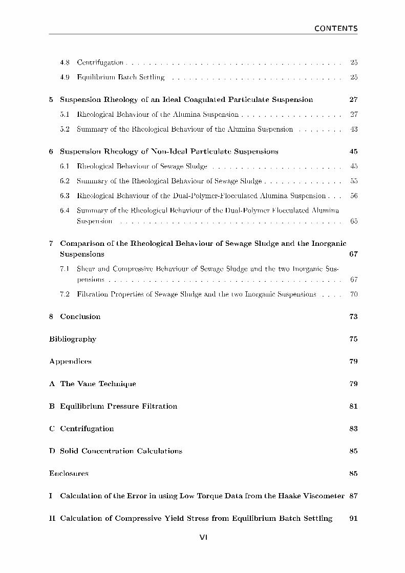
A prediction of Py from τy is especially of interest for systems where compressive yield stressesare dicult to obtain. Sludges are known to be dicult and slow to dewater [Scales et al.,2004]. Characterisation of sludges is furthermore complicated by factors such as bioactivity,health issues, and the fact that they often exhibit non-traditional ltrations behaviour (Figure1.1). Traditional ltration theory is base on a linear correlation between time vs. specic ltratevolume2. This linear region, which correspond to the cake formation region, is very small inthe non-traditional ltration behaviour. This complicates modelling and prediction of ltrationbehaviour of sludges.
Figure 1.1: Non-traditional ltration [Stickland et al., 2007].
Non-traditional ltration has also been observed in a dual occulated alumina suspension [Glover,2003]. The compound in sludge, that is believed to have the major impact on the dewater abilityof sludge, is extra cellular polymers (ECP) [Dignac et al., 2007]. It is believed that the polymersemployed to occulate the alumina suspension have a similar eect.
1.1 Problem Statement
In order to obtain a wide range of compressive and shear yield stresses for a suspension, as afunction of volume fraction, a large sample volume is required. An easily produced sample witha known surface chemistry and high reproducibility is therefore desirable. Mineral suspensionssuch as alumina have previous been investigated with regard to compressive and shear yieldstress with good reproducibility [Zhou, 2000]. The almost incompressible spherical particleswith a narrow size distribution make up an almost ideal system for characterisation. Utilisation
2
1.1 Problem Statement
of such a system enables characterisation of the compressive and shear yield stress for a widevolume fraction range. At the isoelectric point of the suspension (ζ=0) only attractive van derWaals forces are present.
Sludge is known to be dicult to dewater. This makes it dicult to obtain the desired yieldstresses for the material as e.g. sewage sludge from a treatment plant often has a low volumefraction. This needs to be concentrated in order to obtain the dierent volume fractions desiredfor characterisation.
For general characterisation and understanding of sludge behaviour in compression and shear,it would be desirable to create a model system, that exhibits the characteristics of sludge. Inwork done by Glover (2003) non-traditional ltration behaviour, which is a sludge behaviourcharacteristics, has been observed. This work characterised a dual-polymer occulated aluminasuspension.
In this work, an alumina suspension, a occulated suspension, and a sewage sludge will becharacterised. It will not be of interest to optimise or characterise the occulation process for theocculated system. The focus will be on producing a reproducible system for characterisation.Comparison of the three systems will be done with focus on variation in the ratio betweencompressive and shear. This leads to the following problem statement.
How do shear yield stress and compressive yield stress vary with the volume fractionof an alumina suspension, a occulated alumina suspension, and sewage sludge? Isthere a relationship between the determined shear yield stress and compressiveyield stress? What is the correlation between the ratio determined for the aluminasuspension, the occulated alumina suspension, and sewage sludge?
3
Chapter 1. Introduction
4
Chapter 2Microstructure of Suspensions
In this chapter, an introduction to the microstructure of a suspension will be given. The com-pressive and shear yield stress of a suspension are determined by and vary with changes in themicrostructure.
2.1 Forces Acting on Particles in a Suspension
Particles small enough to be unaected by gravity are often dened as colloids. The quantitativedenition of colloids is often particles <1µm. As the densities of the particles vary so will thegravitational eect on these particles and the denition is thus only a generalisation. A colloidin a suspension will constantly undergo thermal randomising motion. It will be inuenced by thesurrounding liquid and interact with the remaining colloids in the suspension. These three forcesacting in a colloidal suspension, called; Brownian forces, hydrodynamic forces, and colloidalforces, respectively, will be explained further.
2.1.1 Brownian Motion
Thermal randomising motion is ever present. This diusive force will try to restore and maintaina random equilibrium distribution of particles in a solution. The equilibrium state of the particledistribution is disturbed when shear is induced in the suspension. This alteration, of the particledistribution caused by introduced shear, is known as the convective eect. The magnitude of thehydrodynamic force determines whether the Brownian motion is able to restore the equilibriumdistribution in the suspension or not. The relative importance of the convection compared todiusion can be expressed by the Peclet number [Hiemenz and Rajagopalan, 1997]:
Pe = 6πη0r3/kBT (2.1)
where η0 is the viscosity of the continuous phase, r is the radius of the particle, kB is Boltzmannconstant, and T is the temperature. At Pe1 diusion in the suspension will dominate andrestore perturbation caused by shear. In the case of Pe1 convection will dominate over diusionand usually cause shear thinning of the liquid which will be discussed in Chapter 3 [Hiemenzand Rajagopalan, 1997].
5
Chapter 2. Microstructure of Suspensions
2.1.2 Hydrodynamic Forces
Hydrodynamic forces are present in owing suspensions and arise from interactions between par-ticles and the owing medium. The viscosity of a suspension is determined by these interactions.The perturbation of the particles in ow eld is responsible for increasing viscosity. In mostcases, deviations from Newtonian behaviour such as shear thinning and shear thickening, areobserved [Mascosko, 1994]. The particle shape, size, concentration, and their ability to deformdetermine the interactions amongst them and thus the resulting viscosity [Barnes, 2000].
2.1.3 Colloidal Interaction
The colloid forces are constituted by the positive van der Waals forces and the negative repulsiveelectrostatic forces.
Van der Waals Interactions
Van der Waals forces are weak long-range (>3nm) interactions that exist between all types ofatoms and molecules. This makes it one of the most important forces when considering surfacechemistry. These attractive forces arise from either permanent or induced dipoles in molecules.In general, three dierent kinds of van der Waals interactions exist. The Keesom interactions(between two permanent dipoles), the Debye interactions (between a permanent dipole and aninduced dipole), and the ever present dispersion (London) forces which exist between two induceddipoles [Hiemenz and Rajagopalan, 1997].The interaction potential between two spherical particles of dierent sizes can be expressed by[Israelachvili, 1992]:
VA = − A
6D
r1 · r2
(r1 + r2)(2.2)
where A is the Hamaker constant, D is the distance between the two particles surfaces, andr1 and r2 are the radius of the two particles. In an ideal system where two similar sphericalparticles are considered this equation can be reduced to:
VA = −A · r12D
(2.3)
in the case where the inter-particle distance between the particles is signicantly smaller thanthe radius of the particle (rD).
Repulsive Electrostatic Forces
Colloids dispersed in an electrolyte solution are often charged. The charges can arise fromdissociated surface groups or from adsorption of ions from the electrolyte solutions to the colloids.The charge of the colloid will attract counter ions. The repulsive force between the co-ions andconstant Brownian motion ensures that the counter ions do not accumulate but instead forman ionic cloud around the colloid surface. As the concentration of the counter ions in the ioniccloud is high, it will together with the surface charge of the colloid form an electrical doublelayer [Ohshima, 2006].
6
2.2 The Electrical Double Layer
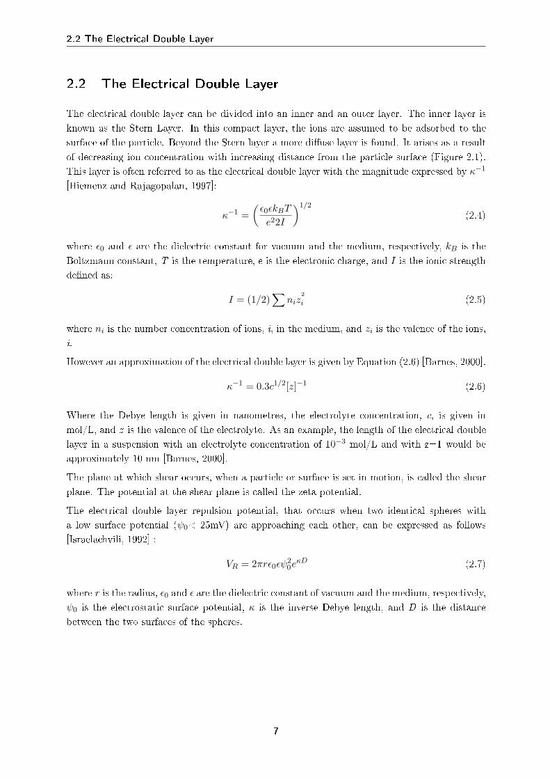
2.2 The Electrical Double Layer
The electrical double layer can be divided into an inner and an outer layer. The inner layer isknown as the Stern Layer. In this compact layer, the ions are assumed to be adsorbed to thesurface of the particle. Beyond the Stern layer a more diuse layer is found. It arises as a resultof decreasing ion concentration with increasing distance from the particle surface (Figure 2.1).This layer is often referred to as the electrical double layer with the magnitude expressed by κ−1
[Hiemenz and Rajagopalan, 1997]:
κ−1 =(
ε0εkBT
e22I
)1/2
(2.4)
where ε0 and ε are the dielectric constant for vacuum and the medium, respectively, kB is theBoltzmann constant, T is the temperature, e is the electronic charge, and I is the ionic strengthdened as:
I = (1/2)∑
niz2
i (2.5)
where ni is the number concentration of ions, i, in the medium, and zi is the valence of the ions,i.
However an approximation of the electrical double layer is given by Equation (2.6) [Barnes, 2000].
κ−1 = 0.3c1/2[z]−1 (2.6)
Where the Debye length is given in nanometres, the electrolyte concentration, c, is given inmol/L, and z is the valence of the electrolyte. As an example, the length of the electrical doublelayer in a suspension with an electrolyte concentration of 10−3 mol/L and with z=1 would beapproximately 10 nm [Barnes, 2000].
The plane at which shear occurs, when a particle or surface is set in motion, is called the shearplane. The potential at the shear plane is called the zeta potential.
The electrical double layer repulsion potential, that occurs when two identical spheres witha low surface potential (ψ0< 25mV) are approaching each other, can be expressed as follows[Israelachvili, 1992] :
VR = 2πrε0εψ20e
κD (2.7)
where r is the radius, ε0 and ε are the dielectric constant of vacuum and the medium, respectively,ψ0 is the electrostatic surface potential, κ is the inverse Debye length, and D is the distancebetween the two surfaces of the spheres.
7
Chapter 2. Microstructure of Suspensions
Figure 2.1: A positively charged surface surrounded mainly by counter ions and the potential as a functionof the distance away from the surface is depicted. The Stern and Diusive layer have a higherpotential than that found in the bulk suspension. The potential at the surface is denoted ψ0 andat the surface of shear it is denoted the zeta potential (ζ). Furthermore, the potential at the Sternplane (ψδ) and at the diuse layer boundary (ψd) is dened.
2.3 DLVO theory
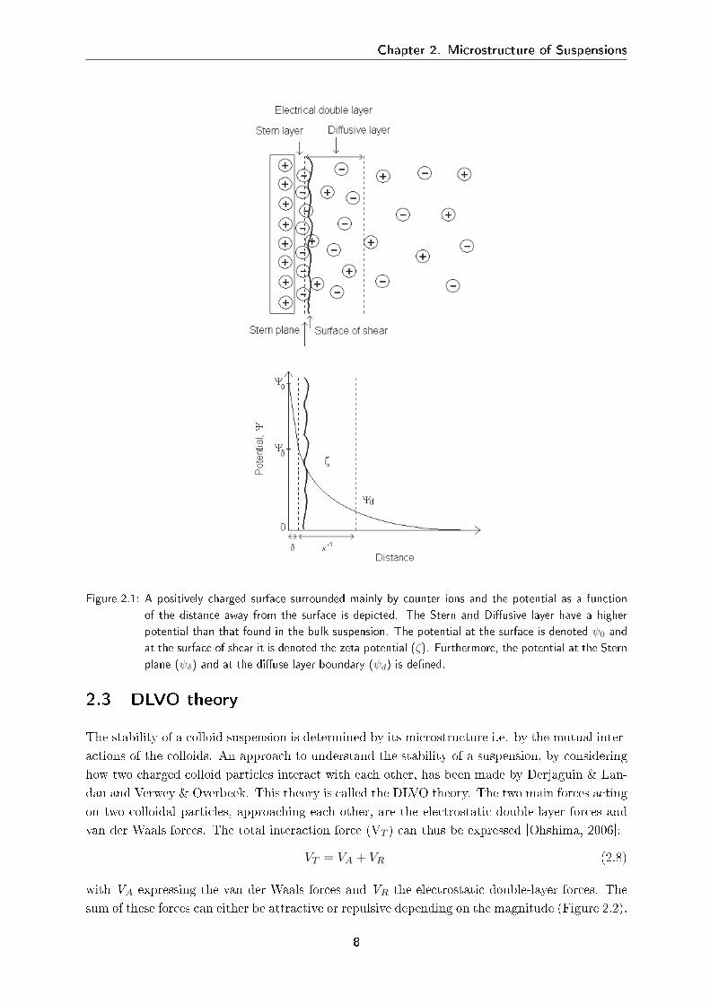
The stability of a colloid suspension is determined by its microstructure i.e. by the mutual inter-actions of the colloids. An approach to understand the stability of a suspension, by consideringhow two charged colloid particles interact with each other, has been made by Derjaguin & Lan-dau and Verwey & Overbeek. This theory is called the DLVO theory. The two main forces actingon two colloidal particles, approaching each other, are the electrostatic double-layer forces andvan der Waals forces. The total interaction force (VT ) can thus be expressed [Ohshima, 2006]:
VT = VA + VR (2.8)
with VA expressing the van der Waals forces and VR the electrostatic double-layer forces. Thesum of these forces can either be attractive or repulsive depending on the magnitude (Figure 2.2).
8
2.3 DLVO theory
The DLVO theory uses the resulting potential energy to explain the stability of the suspension.It is assumed that the motion of the colloid is negligible compared to the motion of the electrolyteions. The two colloids can thus be considered to be at a xed distance from each other, with theelectrolyte ions moving around them [Ohshima, 2006].
For two identical particles the total interaction energy can be expressed by:
VT = −A · r12D
+ 2πaε0εψ20e
κD (2.9)
where A is the Hamaker constant, D is the distance between the two surfaces of the particles,r is the radius, ε0 and ε are the dielectric constant of vacuum and the medium, respectively,ψ0 is the electrostatic surface potential, and κ is the inverse Debye length. From Equation(2.9), it can be deduced that the attractive van der Waals forces decay with the inverse powerof the distance (x) from the particle surface, and that the repulsive double layer forces decayexponentially. As a consequence, the attractive van der Waals forces will often either dominatethe total interaction energy at all distances (x) or both at short and long distances. In the caseof the latter, the repulsive electrical double layer forces will constitute an energy barrier, to beovercome, before particle coagulation can occur. If Equation (2.7) is considered (and the liquidmedium is unchanged) the magnitude of this energy barrier is determined by two parameters.The potential at the Stern plane (ψD ≈ ζ) and the Debye length (κ−1) which can be related tothe surface chemistry of the suspension including the pH and the ionic strength. At the isoelecticpoint (IEP) of a suspension (the pH where ζ=0) the repulsive electrical double layer forces arenon-existing (Figure 2.2e). In the case where the zeta potential is high and/or the ionic strengthis low, a high energy barrier exists. If the energy barrier is insurmountable by thermal energy,the suspension will be dispersed and colloid stability occur. At low zeta potential and/or highionic strength the energy barrier is low and if the thermal energy of the particles is high enoughto overcome the barrier and reach the primary minimum, coagulation will occur.
Figure 2.2: The DLVO theory picturing the attractive van der Waals forces (VA), the repulsive double-layerinteractions (VR), and the sum of these (VT ). The numbers from a-e show the eect of increasingsalt which result in a decreasing surface potential.
9
Chapter 2. Microstructure of Suspensions
2.4 Non-DLVO Forces
At short separation distances (<3nm), other forces than van der Waals and DLVO forces be-comes more signicant. In other words the DLVO theory fails to describe short range interactions.Attractive non-DLVO forces, including bridging and depletion forces, often arise in occulatedsuspensions. As the terms coagulation and occulation often are used indiscriminately, a dis-tinction between them will be made in this work to minimise confusion. Coagulation describesthe phenomenon where particles are driven together by means of chemical additives resulting ina diminished repulsion and a dominant attraction between the particles. An example, is addingacid or base to change pH and reach the IEP point. At the IEP the particles have no chargeand thus no electric double layer repulsive force exists. Flocculation, on the other hand, is inthis work used to describe aggregation of particles caused by addition of high molecular weightpolymers.
2.4.1 Bridging Forces
The phenomenon of bridging occurs when a polymer is adsorbed to more than one particlesurface. A technique often used to occulate particles in order to improve solid-liquid separationprocesses. A low degree of surface coverage by the adsorbing polymers in the suspension enhancesthe possibility of bridging [Israelachvili, 1992; Johnson et al., 2000].
2.4.2 Depletion Forces
Attraction between two particles can arise due to depletion forces. A particulate suspension, witha non absorbing low molecular weight polymer, is considered. When the particles are separated,with a larger distance than the radius of the polymer, there is no net force between the particles.The dispersed polymer molecules will exert an osmotic pressure on all sides of the particles. Inthe case where the two particles are in closer proximity, such that the distance between them issmaller than the radius of the polymer molecules, the polymer molecules are excluded from theclose contact area. An osmotic pressure is exerted on the remaining part of the particles leadingto a net attractive force between the particles [Hiemenz and Rajagopalan, 1997].
10
Chapter 3Rheology of Suspensions
Rheology of particulate uids is more complicated than rheology of pure uids. As concentrationin a particulate uid is increased the particles will interact with each other and form a threedimensional network structure. This structure will be able to store some energy elastically andthe suspension will have a yield stress. The yield stress is the minimum stress required to breakdown this three dimensional network structure.
3.1 Denition of Viscoelastic Behaviour
Particulate uids are viscoelastic materials as they exhibit both elastic and viscous properties.If a stress below the yield stress is applied to the suspension, the suspension will act elastic andstore all the energy applied to the suspension. After removal of the stress complete spontaneousrecovery of the deformation will result. On the other hand, if a suspension is deformed suchthat the three dimensional network is broken down, the suspension will start to ow at a criticalstress (shear yield stress, τy). The time scale at which experiments are observed is thus thedetermining factor of how the suspension will behave.
This can be explained by the dimensionless Deborah number (De) which is dened as [Goodwinand Hughes, 2000]:
De =tr (stress relaxation time)t (observation time) (3.1)
the stress relaxation time (tr) can be dened as the time it takes for the molecules in a deformedsuspension to diuse from the higher energy state, which they have been shifted to during thedeformation, to a lower energy equilibrium state. If the observation time is signicant longerthan the stress relaxation time, diusion will have occurred and the suspension will then havelost its initial shape and started to ow and behave liquid-like (De1). In the other case, wherethe stress relaxation time is signicantly longer than the observation time, the suspension willappear solid-like as no diusion has occurred and all the energy is stored in the suspension(De1). In most cases both behaviours will be observed [Goodwin and Hughes, 2000].
11
Chapter 3. Rheology of Suspensions
3.2 Viscosity of Suspensions
The viscosity of very diluted suspensions is not of interest for this work. The concentration awhich the particles in a suspensions start forming a network is dened as the gel point (φ(g)).Concentrations from the gel point to the maximum packing fraction (φcp) are those of interest.
The simplest ow behaviour, for yield stress materials is the ideal plastic ow (Bingham plasticbehaviour) which is described with the Bingham model:
τ = τB + ηpl·γ, τ ≥ τB (3.2)
that suggests a linear relationship between shear rate (·γ) and shear stress (τ) above the Bingham
yield stress (τB) with the slope of the line being the viscosity (ηpl) describing the viscoplasticow. Equation (3.2) assumes that the structure, which can resist irreversible deformation, breaksdown completely the moment the yield stress is applied or exceeded. However, this behaviour isin most cases only observed at high shear rates, which can indicate that in most suspensions agradual degradation of the network during shear is the case, rather than an instant degradation.An empirical model to describe a nonlinear dependence has been proposed by Herschel andBulkley (1926):
τ = τHB + k·γ
m, τ ≥ τHB (3.3)
with τ being the shear stress, τHB the yield stress,·γ the shear rate and, m and k constants and
power law parameters often used to describe ow behaviour. If the viscosity declines with shearrate, m<1, the suspension is classied as yield-pseudo plastic. At m=1 the equation reducesto the Bingham model (Equation (3.2)). If the viscosity is increasing, m>1, the suspension isclassied as yield-dilatant plastic. Another model to describe a nonlinear dependence has beenproposed by Casson (1959):
τ1/2 = τ1/2C + (η∞
·γ)1/2, τ ≥ τC (3.4)
This model includes only two parameters beside the shear stress (τ) and the shear rate (·γ):
the Casson yield stress (τC) and the constant viscosity obtained at an innite shear rate (η∞)[Nguyen and Boger, 1992].
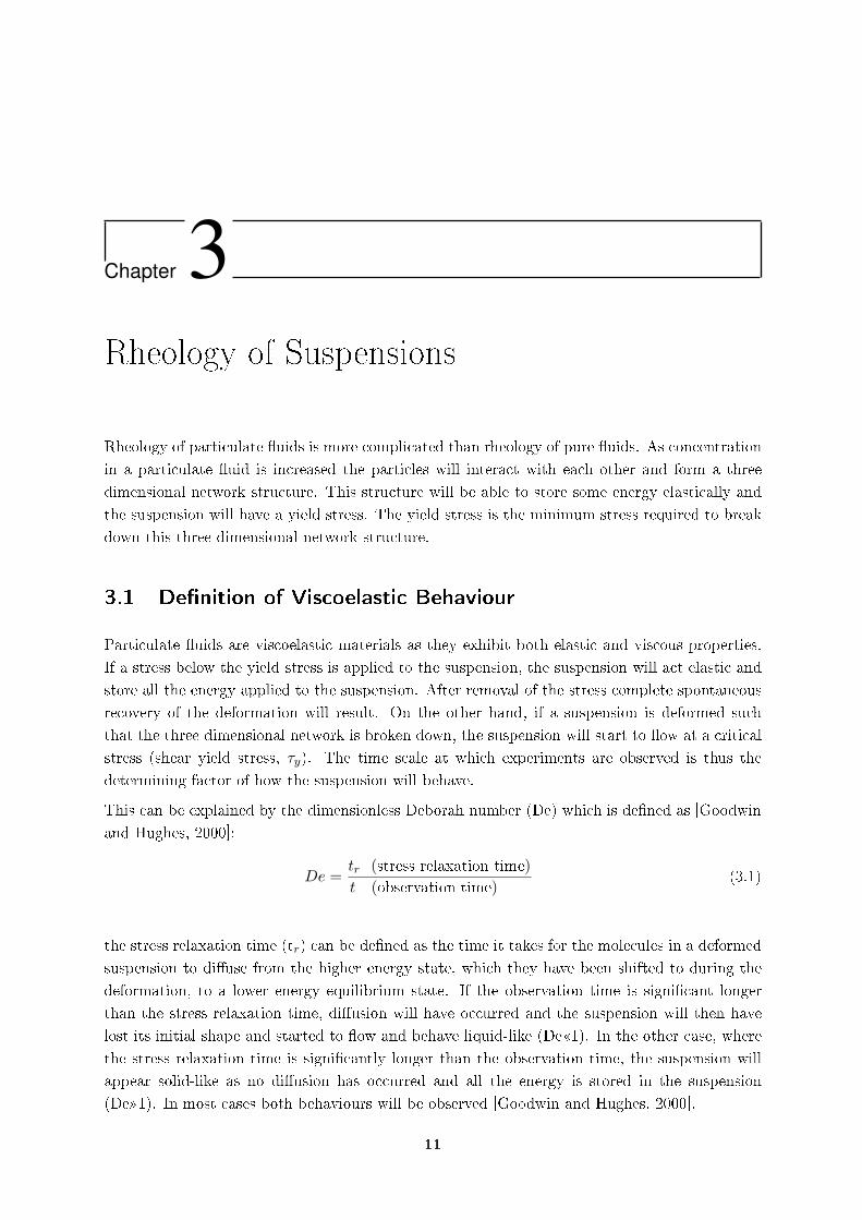
The three kinds of dierent viscosities can be viewed in Figure 3.1.
12
3.2 Viscosity of Suspensions
Figure 3.1: Flow behaviour of plastic material. Ideal plastic ow exhibit a yield stress followed by a lineardependence of shear stress on shear rate. Shear thinning behaviour beyond the yield stress isnoted yield-pseudo plastic and shear thickening beyond the yield stress yield-dilatant.
3.2.1 Shear Thinning or yield Psudoplastic Behaviour
Shear thinning properties are often observed in colloidal suspensions. In aggregated suspensionsdominated by attractive forces, the decrease in viscosity with shear rate is believed to be due toaggregates either breaking up or densifying. The microstructure can be used to explain this, asBrownian motion dominates at low shear rates and maintain the equilibrium structure whereashydrodynamic forces dominate at high shear rates, rearranging or altering the aggregate structureresulting in altered ow [Ackerson, 1990].
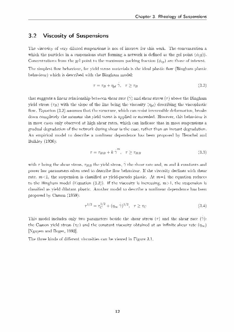
At low shear rates, Brownian motion maintains random distributed particles but as the shearrates is increased convection becomes dominant (Pe1) and particles arrange in string like struc-tures as illustrated in Figure 3.2 [Barnes, 2000].
Figure 3.2: Spatial arrangement of particles which when non sheared is dominated by Brownian motion andduring shear form string like structures, that make ow occur easier and promote shear thinning[Barnes, 2000]
The string like arrangement of the particles at high shear rate decreases the distance betweenthe particles in the ow direction, and increases the distance between the particle layers whichpromotes ow and yield shear thinning. In some cases the decrease in viscosity can be followed byan increase in viscosity i.e. shear thickening behaviour at high shear rates. The further increasein shear rate/stress can result in a break down of the previous formed string like structures tolumps or the strings can be aligned crosswise to the ow direction, which in both cases lead toan increase in viscosity.
13
Chapter 3. Rheology of Suspensions
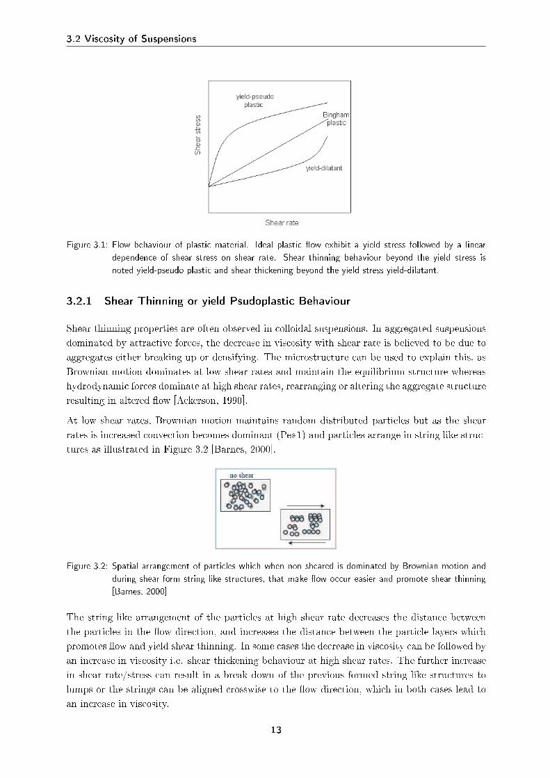
The shear thinning eect is greater for larger particles, as these are less inuenced by Brownianmotion and will be arranged more easily. This is illustrated in Figure 3.3.
Figure 3.3: The eect of particle size on the viscosity. Small particles are more inuenced by Brownian motionwhich maintain random distributed particles and maintain a higher viscosity compared to theviscosity of larger particles [Barnes, 2000]
The Peclet number accounts for the relative inuence of Brownian motion versus convection.The viscosity as a function of the Peclet number is thus the same for dierent sizes particles.
3.2.2 Shear Thickening or yield Dilatant Behaviour
An increase in viscosity as a function of shear rate is called shear thickening behaviour. Thistype of behaviour is often encountered in highly concentrated uids and an explanation is givenforthwith. In concentrated uids, high density packing of the particles allows only a smallquantity of liquid between the particles. When the suspension is sheared at low shear rates thisliquid is enough to lubricate the motion of particle past each other. At higher shear rates, thedense packing breaks down and the suspension expands resulting in a solid-solid friction. Due tolack of liquid between the particles, which causes the stress to increase more rapidly and thus theviscosity increases more rapidly. As is the case with shear thinning behaviour, shear thickeningbehaviour can often be modelled by a straight line on a log-log scale of shear rate vs. shear stressand Equation (3.3), where m>1 can thus be employed to model this behaviour [Barnes, 2000].
3.3 Time-Dependent Behaviour
Changes in the microstructure of a suspension as a result of shear do not take place instanta-neously in any suspension, but in most cases the utilized viscometers are too slow to measure theshort delay. For some suspensions, the response takes longer and the suspension is said to have atime dependent behaviour. Shear history of the suspension will then aect the measurement ofrheological properties. The ow properties can be aected by both shear rate and time of shear-ing. Two types of time-dependent behaviour can be experienced; Thixotropy or anti-thixotropy(rheopexy) [Barnes, 1997].
14
3.4 Shear Yield Stress
3.3.1 Thixotropy
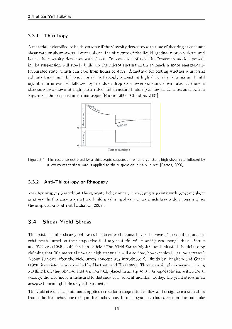
Amaterial is classied to be thixotropic if the viscosity decreases with time of shearing at constantshear rate or shear stress. During shear, the structure of the liquid gradually breaks down andhence the viscosity decreases with shear. By cessation of ow the Brownian motion presentin the suspension will slowly build up the microstructure again to reach a more energeticallyfavourable state, which can take from hours to days. A method for testing whether a materialexhibits thixotropic behaviour or not is to apply a constant high shear rate to a material untilequilibrium is reached followed by a sudden drop to a lower constant shear rate. If there isstructure breakdown at high shear rates and structure build up at low shear rates as shown inFigure 3.4 the suspension is thixotropic [Barnes, 2000; Chhabra, 2007].
Figure 3.4: The response exhibited by a thixotropic suspension, when a constant high shear rate followed bya low constant shear rate is applied to the suspension initially in rest [Barnes, 2000].
3.3.2 Anti-Thixotropy or Rheopexy
Very few suspensions exhibit the opposite behaviour i.e. increasing viscosity with constant shearor stress. In this case, a structural build up during shear occurs which breaks down again whenthe suspension is at rest [Chhabra, 2007].
3.4 Shear Yield Stress
The existence of a shear yield stress has been well debated over the years. The doubt about itsexistence is based on the perspective that any material will ow if given enough time. Barnesand Walters (1985) published an article "The Yield Stress Myth?" and initiated the debate byclaiming that 'if a material ows at high stresses it will also ow, however slowly, at low stresses'.About 70 years after the yield stress concept was introduced for uids by Bingham and Green(1920) its existence was veried by Hartnett and Hu (1989). Through a simple experiment usinga falling ball, they showed that a nylon ball, placed in an aqueous Carbopol solution with a lowerdensity, did not move a measurable distance over several months. Today, the yield stress is anaccepted meaningful rheological parameter.
The yield stress is the minimum applied stress for a suspension to ow and designates a transitionfrom solid-like behaviour to liquid like behaviour. In most systems, this transition does not take
15
Chapter 3. Rheology of Suspensions
place instantaneously but occurs over a range of stresses in which the material exhibits viscoelasticbehaviour (also referred to as viscoplastic ow). This observation leads to the denition of twodierent yield stresses; the transition from a solid-like behaviour to a viscoelastic behaviour andthe transition from a viscoelastic behaviour to a liquid-like behaviour often denoted the static andthe dynamic yield, respectively. The three dimensional structure formed, above the gel point, ina suspension is believed to be responsible for the ability of a suspension to elastically resist lowstresses. As the stress is increased this three dimensional structure will gradually break downand in the end nally allow viscous ow to occur. Therefore, the yield stress can be viewed asthe force per unit area it takes to break down the three dimensional network [Liddell and Boger,1995].
The shear yield stress can be measured with a number of dierent techniques that are eitherclassied as direct or indirect. Indirect techniques often extrapolate shear stress-shear rate datato a zero shear rate by means of models which means that the techniques employed are techniquesnormally used to measure viscosity (Section 3.2). To obtain accurate estimation of the yield stressby extrapolating data, the data in the low shear rate region should be known. However, whenusing conventional rheometers such as a capillary rheometer or a Weissenberg rheogoniometer itis often dicult to measure low shear rate data due to problems such as wall slip. In a suspensionconsisting of smooth spherical particles, for example, the distribution of the particles in the bulksuspension will be random. However, at the wall, the particle concentration will be zero and arapid increase in concentration will be observed when moving away from the wall. This resultsin wall slip (wall depletion) [Barnes et al., 1989]. The problem is mostly observed at low shearrates.
The direct methods measure a dened yield stress. This can be the transition between elasticbehaviour and plastic behaviour or the transition between plastic deformation and start of viscousow behaviour. The three most common techniques for measuring yield stress directly arecreep/recovery, stress relaxation, or stress growth experiments. In creep/recovery experiments,dierent constant stresses are applied to the suspension for a dened period of time and thenremoved. An applied stress below the yield stress leads to a constant strain value with time andcomplete recovery after removal of the stress. The yield stress is dened as the stress where thestrain increases indenitely i.e. the point where the suspension starts to ow and incompletestrain recovery is obtained after removal of the stress.
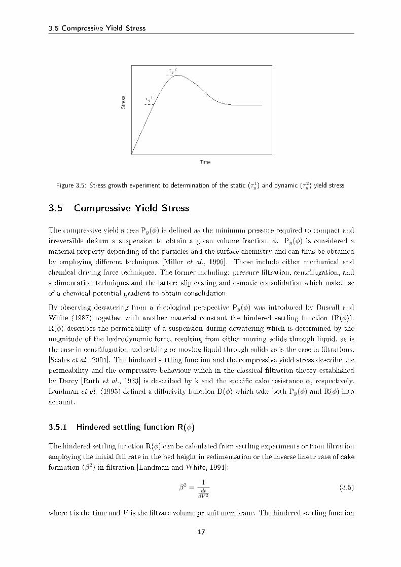
In the stress growth experiments the suspension is sheared at a low constant shear rate and theyield stress (transition from viscoelastic to viscous behaviour) is dened as the maximum stressobtained in a stress-time prole, i.e. the point at which the three dimensional structure breaksdown and the suspension starts to ow (Figure 3.5).
16
3.5 Compressive Yield Stress
Figure 3.5: Stress growth experiment to determination of the static (τ1y ) and dynamic (τ2
y ) yield stress
3.5 Compressive Yield Stress
The compressive yield stress Py(φ) is dened as the minimum pressure required to compact andirreversible deform a suspension to obtain a given volume fraction, φ. Py(φ) is considered amaterial property depending of the particles and the surface chemistry and can thus be obtainedby employing dierent techniques [Miller et al., 1996]. These include either mechanical andchemical driving force techniques. The former including: pressure ltration, centrifugation, andsedimentation techniques and the latter: slip casting and osmotic consolidation which make useof a chemical potential gradient to obtain consolidation.
By observing dewatering from a rheological perspective Py(φ) was introduced by Buscall andWhite (1987) together with another material constant the hindered settling function (R(φ)).R(φ) describes the permeability of a suspension during dewatering which is determined by themagnitude of the hydrodynamic force, resulting from either moving solids through liquid, as isthe case in centrifugation and settling or moving liquid through solids as is the case in ltrations.[Scales et al., 2004]. The hindered settling function and the compressive yield stress describe thepermeability and the compressive behaviour which in the classical ltration theory establishedby Darcy [Ruth et al., 1933] is described by k and the specic cake resistance α, respectively.Landman et al. (1995) dened a diusivity function D(φ) which take both Py(φ) and R(φ) intoaccount.
3.5.1 Hindered settling function R(φ)
The hindered settling function R(φ) can be calculated from settling experiments or from ltrationemploying the initial fall rate in the bed height in sedimentation or the inverse linear rate of cakeformation (β2) in ltration [Landman and White, 1994]:
β2 =1dt
dV 2
(3.5)
where t is the time and V is the ltrate volume pr unit membrane. The hindered settling function
17
Chapter 3. Rheology of Suspensions
can then be calculated 3.6 [Landman et al., 1999]:
R(φf ) =λ
VPr(φ) =
2dβ2
d∆P
(1φ0− 1
φf
)(1− φf )2 (3.6)
where λ is Stoke's drag coecient for a single particle, VP denotes the volume of a single particle,r(φ) is the hindered settling factor, φ0 is the initial volume fraction, φf is the nal volume fraction,and dβ2
d∆P is the slope of a plot of β2 vs. ∆ P.
3.5.2 Solids diusivity D(φ)
The solids diusivity D(φ) can be either calculated from knowledge of R(φ), the slope of Py(φ)vs. φ, and the nal volume fraction (φf ) or from the slope of β2 vs. φf , φ0 and φf [Landman etal., 1999]:
D(φf ) =dPy(φ)
dφ
(1− φf )2
R(φf )=
12
dβ2
dφf
(1φ0− 1
φf
)−1
(3.7)
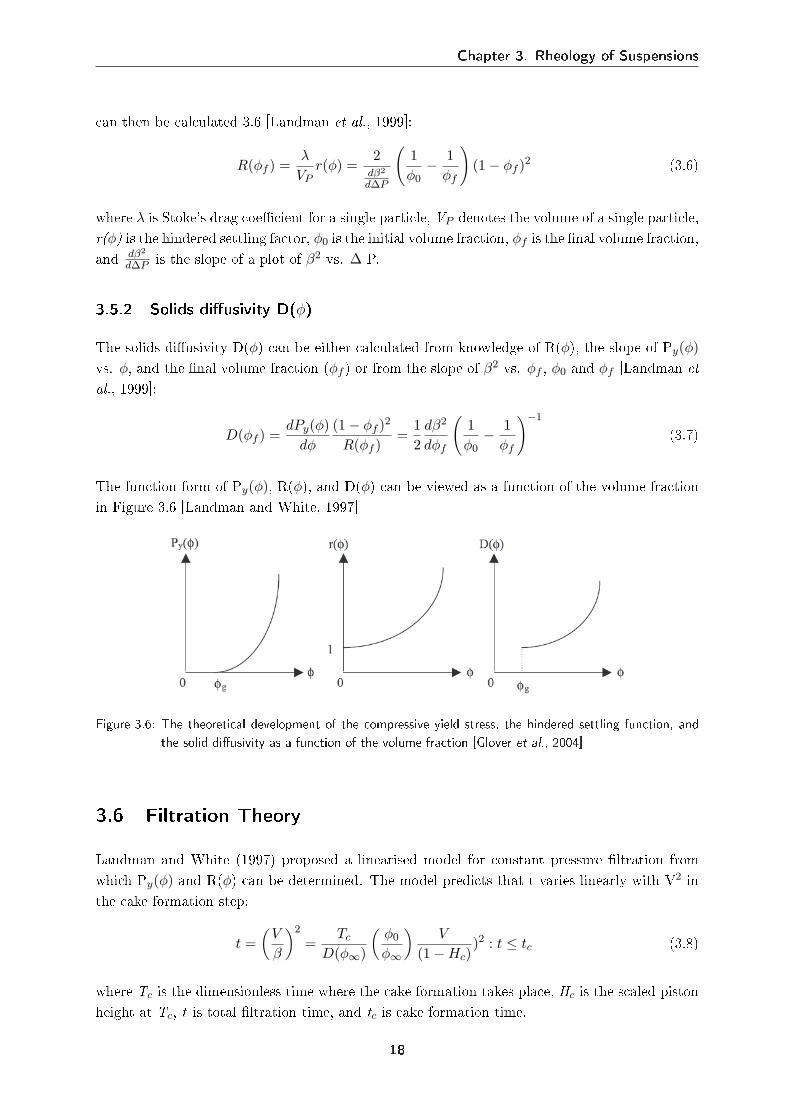
The function form of Py(φ), R(φ), and D(φ) can be viewed as a function of the volume fractionin Figure 3.6 [Landman and White, 1997]
Figure 3.6: The theoretical development of the compressive yield stress, the hindered settling function, andthe solid diusivity as a function of the volume fraction [Glover et al., 2004]
3.6 Filtration Theory
Landman and White (1997) proposed a linearised model for constant pressure ltration fromwhich Py(φ) and R(φ) can be determined. The model predicts that t varies linearly with V2 inthe cake formation step:
t =(
V
β
)2
=Tc
D(φ∞)
(φ0
φ∞
)V
(1−Hc))2 : t ≤ tc (3.8)
where Tc is the dimensionless time where the cake formation takes place, Hc is the scaled pistonheight at Tc, t is total ltration time, and tc is cake formation time.
18
3.6 Filtration Theory
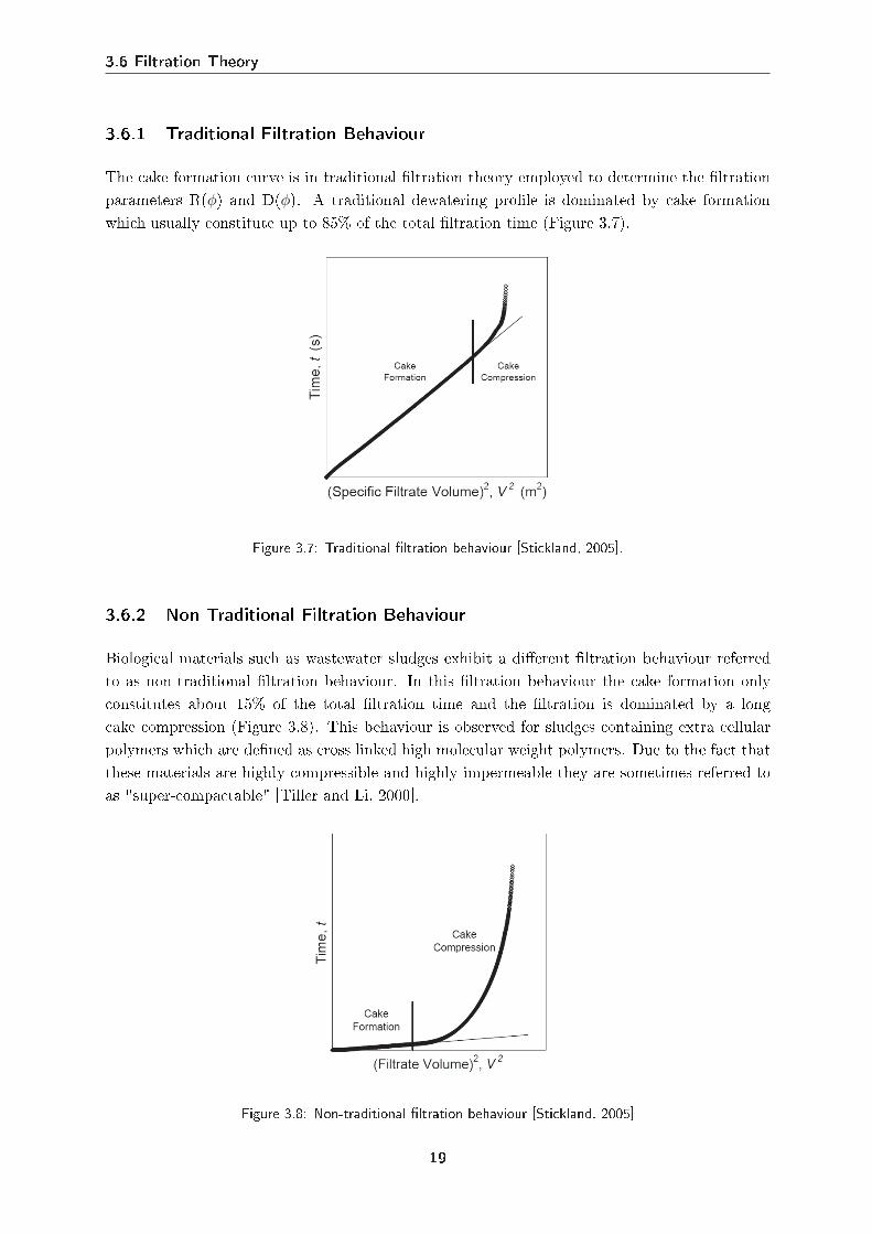
3.6.1 Traditional Filtration Behaviour
The cake formation curve is in traditional ltration theory employed to determine the ltrationparameters R(φ) and D(φ). A traditional dewatering prole is dominated by cake formationwhich usually constitute up to 85% of the total ltration time (Figure 3.7).
Figure 3.7: Traditional ltration behaviour [Stickland, 2005].
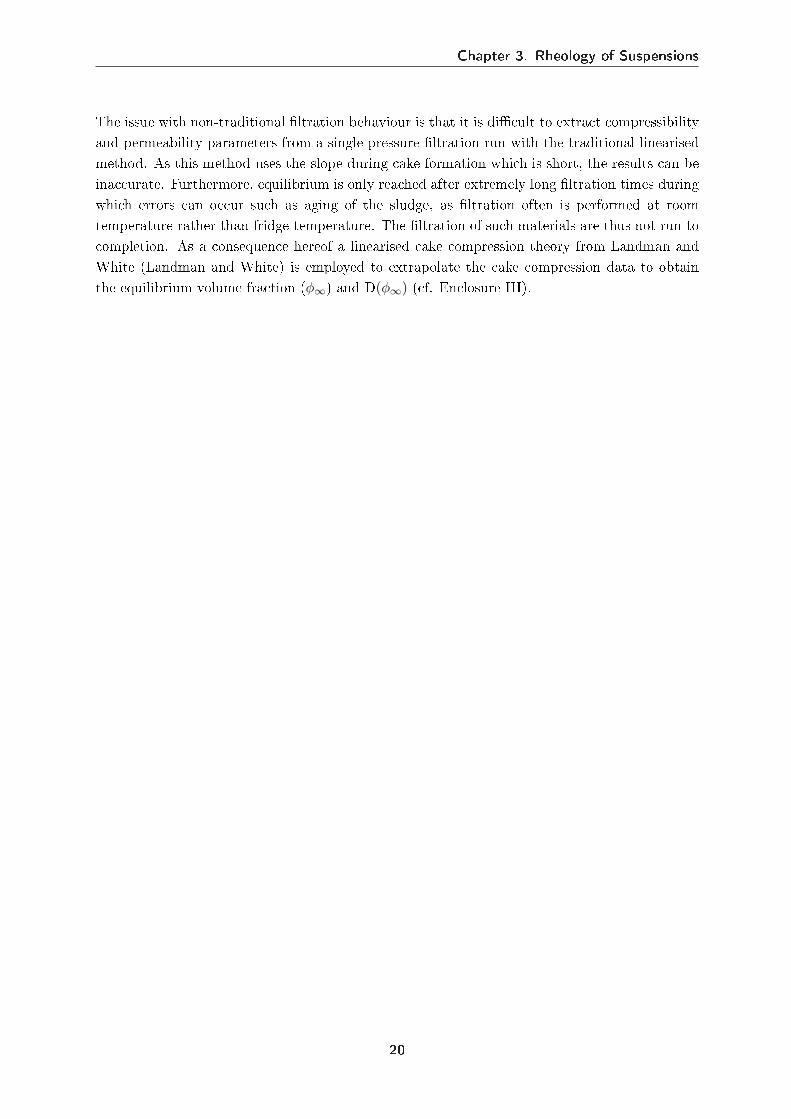
3.6.2 Non-Traditional Filtration Behaviour
Biological materials such as wastewater sludges exhibit a dierent ltration behaviour referredto as non-traditional ltration behaviour. In this ltration behaviour the cake formation onlyconstitutes about 15% of the total ltration time and the ltration is dominated by a longcake compression (Figure 3.8). This behaviour is observed for sludges containing extra cellularpolymers which are dened as cross linked high molecular weight polymers. Due to the fact thatthese materials are highly compressible and highly impermeable they are sometimes referred toas "super-compactable" [Tiller and Li, 2000].
Figure 3.8: Non-traditional ltration behaviour [Stickland, 2005]
19
Chapter 3. Rheology of Suspensions
The issue with non-traditional ltration behaviour is that it is dicult to extract compressibilityand permeability parameters from a single pressure ltration run with the traditional linearisedmethod. As this method uses the slope during cake formation which is short, the results can beinaccurate. Furthermore, equilibrium is only reached after extremely long ltration times duringwhich errors can occur such as aging of the sludge, as ltration often is performed at roomtemperature rather than fridge temperature. The ltration of such materials are thus not run tocompletion. As a consequence hereof a linearised cake compression theory from Landman andWhite (Landman and White) is employed to extrapolate the cake compression data to obtainthe equilibrium volume fraction (φ∞) and D(φ∞) (cf. Enclosure III).
20
Chapter 4Materials and Methods
4.1 Preparation of Alumina Suspensions
The alumina (APK-30) (Aluminum Oxide 99.99%, Al2O3, Sumitomo Shoji Chemicals Co.,Tokyo, Japan) suspensions were prepared according to the method utilized by Zhou (2000).The powder was mixed with a 0.01M KNO3 (Potassium nitrate 99.0%, BDH Laboratory Sup-plies Poole, England) solution, with a conductivity of about 1500 µS/cm, and the desired volumefraction prepared. The mixing was performed with a spatula and the suspensions were mixeduntil all particles were wetted. After mixing, the suspension was sonicated at 200 Watt (BransonSonier 450) for 2 minutes to break up any lumps. The pH was adjusted, to a value of 5 (PHM92 pH meter, Radiometer Copenhagen, Denmark) where the suspension was fully dispersed, andit was then further sonicated for another minute. The suspension was then allowed to rest for 24hours to achieve chemical and physical equilibrium. Before measurements, the pH was adjustedto 9.0±0.1 and allowed to rest for two hours. The acid and base used in the pH adjustmentwere 1M Nitric Acid (HNO3, 69%, Merck Pty Limited, Kilsyth, Australia) and 1M PotassiumHydroxide (KOH, Chem supply, Gillman, South Australia). Dierent volume fractions were ob-tained by diluting a stock suspension with 0.01M KNO3 solution and adjusting pH. The volumefraction was determined by weight loss on drying, where the samples were left to dry for 24 hourat 100C (Lab-line Due-Vac oven, Melrose Park,ILL) (cf. Appendix D).
4.2 Preparation of Sewage Sludge Suspensions
The sewage sludge was a mesophilic anaerobically digested sewage sludge from the eastern treat-ment plant, Carrum, Victoria (Melbourne Water), collected 27. Aug 2007. It was stored at4C to avoid bacterial degredation. The sewage sludge had an initial volume fraction of 0.0097v/v, pH=7.09, and a conductivity of 6.69 µS/cm. Higher volume fractions were attained bycentrifugation (Jouan CT 422) at 4C where the water was removed after centrifugation.
21
Chapter 4. Materials and Methods
4.3 Preparation of Dual-Polymer Flocculated Alumina Suspen-sions
Alumina suspensions were occulated with polyacrylic acid and a polyacrylamide polymer.
Alumina suspensions with an electrolyte concentration of 10−3M KNO3 were prepared accordingto Section 4.1. Diluted suspensions for occulation were prepared by diluting the stock suspensionto a 2.5 w/w% suspension with 10−3M KNO3 solution. The diluted dispersions were thensonicated for 1-2 min and left overnight to reach chemical equlibrium and the pH was adjustedto 7.29 ± 0.1. The conductivity was 183±12 µS/cm.
4.3.1 Preparation of Polymer Solutions
A 0.1% wt solution of polyacrylic acid (PAA 250,000 g/mol, Aldrich Chemical Company, USA)was prepared by dissolving PAA in demineralised water. The solution was stirred 1 hour, toensure complete dissolution of the polymer, using a magnetic stirrer.
A 2 g/L stock polymer solution of non-ionic polyacrylamide (Magnaoc LT20, ca. 10-15 mill.g/mol) was produced by dissolving 0.2 g of Magnaoc LT20 (Allied Colloids, Australia) in 2 mLof ethanol (Merck Pty Limited, Kilsyth, Australia) and diluting with 98 mL of demineralisedwater. To ensure mixing, the solution was shaken vigorously for 1 minute and then left on anend-to-end rotating table, covered in aluminum foil to avoid UV degradation of the polymer,overnight. 1 hour before occulation, a 0.01% wt diluted solution was produced by diluting thestock solution as follows: 25 mL of stock solution was transferred to a beaker and mixed with250 mL of tap water whereupon 225 mL of demineralised water was added and the solution wasstirred 1 hour using a magnetic stirrer.
4.3.2 Flocculation Procedure
The occulation was preformed in a bae reactor (Figure 4.1). The 2.5 w/w % suspension wasdecanted to the bae reactor and the suspension was mixed for minimum ve minutes at 500rpm (Heidolph, RZR 2020 control) to achieve a homogeneous mixture. Prior to occulation,the speed was reduced to 330 rpm. PAA was rst added, through the inlet tube with a plasticsyringe, and left to mix for 1 minute before the second polymer Magnaoc LT20 was added tothe suspension and further 20 sec of mixing was performed. The suspension was left for ocsto settle and the settling rate was determined using a stop watch. After the ocs have settled,the stirrer and the baes were removed from the suspension and the supernatant was gentlyremoved using a syringe.
22
4.4 Density, Conductivity and Size Measurements
Figure 4.1: Flocculation setup with bae reactor and Rushton impeller [Hulston, 2005].
4.4 Density, Conductivity and Size Measurements
The density was measured using a 50 cm3 density glass bottle where the lid contained a smallhole in the middle to allow excess uid to exit (Duran). The volume of the glass bottle wasdetermined using water at a known temperature. The glass bottle was then lled with thesample. The mass of the sample together with a known mass fraction of the liquid sample enablescalculation of the solid density of the particles (cf. Appendix D). Suspension conductivitywas measured with (IONcheck65, Radiometer analytical). Particle size was measured with aMastersizer (Mastersizer2000, Hydro 2000G, Malvern Instruments).
4.5 Scanning Electron and Optical Microscopy
Before Scanning electron microscopy (SEM, FEI Quanta 200 FEG) was utilised, the sampleswere gold coated with 10 nm of gold (1 minute of coating) using a Gold sputter mini coater(Dynavac, Australia) with associated vacuum pump (Edwards Model RV3, England). The opticalmicroscopy used was Olympus (U-CMAD-2, Japan).
4.6 The Vane Technique
Shear yield stress and viscosity was measured with a vane on a Haake Viscometer (HAAKEVT550, Kahlsruhe, Germany) and an Advanced Rheological Expansion System rheometer (ARES,TA. Inc., New Castle, USA). The dierent vane dimensions employed are shown in Table 4.1.
23
Chapter 4. Materials and Methods
Table 4.1: The dierent vane geometries employed to measure the shear yield stress of a suspension.Vane Height (H) Diameter (Dv)
[· 10−3 m] [· 10−3 m]1 15.145 9.962 20.2025 20.21253 30.1725 25.024 50.0 25.05 75.0 25.06 100 507 200 100
The yield stress measurement was performed by loading the sample in a suitable container andshearing it well to avoid potential thixotropic eects that would inuence the results. Thevane is lowered into the suspension until the suspension covers the vane, plus a further distancecorresponding to the vane radius. Then a shear rotation rate of 0.2 Ω [ 1
min ] was applied and theyield stress was calculated (cf. Appendix A) .
4.6.1 Procedure for Measuring High Shear Yield Stress
Due to the diculty of preparing high volume fraction suspensions, ltration was utilised. Twoinstruments were used to measure the yield stress of the resulting volume fractions; namely theHaaake viscometer and the ARES rheometer. The ARES was used to measure the higher yieldstresses as the Haake viscometer has a limiting torque of about 30,000 µNm corresponding to astress of about 10,000 Pa when the smallest vane (vane 1) is employed. The ARES has a limitingtorque of 100,000 µNm corresponding to a stress about 35,000 Pa (vane 1). The yield shear stressmeasured with the Haake viscometer could be measured directly in the ltration rig whereas thesuspension had to be placed in a special cup when measured with the ARES rheometer asthe vane is xed in these measurements and the cup is rotating. To avoid disturbance of thesample caused by immersion of the vane, the vane was left in the sample 2 minutes prior to themeasurement.
4.7 Equilibrium Pressure Filtration
A piston rig that uses a linear encoder to monitor piston height was used.
The piston was greased and set equal to the initially desired sample height. The rig was assembledusing a membrane and the membrane wetted. The sample was then loaded in the ltration rigand the ltration rig closed and lowered to the correct position. The desired pressures werechosen and the airow connected. The nal volume fraction was determined by weight loss ondrying.
24
4.8 Centrifugation
4.8 Centrifugation
Clear, round bottomed, polycarbonate centrifuge tubes (height: 103 mm, inside diameter: 26.5mm) (Naglene) were employed for the concentration prole technique. A constant radial stressdistribution is required which was gained by attening the bottom of the centrifuge tubes withepoxy resin. The measurement was then performed by measuring the initial height of the tubes.As the epoxy resin was not completely even, the height was determined with a steel ruler (pre-cision 0.1 mm, Digital Caliper) from an average value of six measurements round the tube. Thetubes were then loaded with sample at a desired volume fraction and initial sample heights be-tween 7-50 mm. The alumina suspensions were tested at 20C, whereas the sludge was run at4C to prevent bacterial growth. The samples were run until equilibrium was obtained, whichwas ensured by measure of the bed height until constant. As the height was not even an averageof the height measured six places along the tube was calculated. When the centrifugation wascomplete the nal sample was divided into about 10 slices. Each sub-sample was removed byscraping the sample from the tube using a at spatula xed at the desired sample height andthe volume fraction for the sub-sample was found by weight loss on drying (Figure 4.2).
Figure 4.2: Schematic overview of the concentration prole technique after centrifugation. Ht is the totalheight of the tube and Hs is the height at which the scrape is taken.
4.9 Equilibrium Batch Settling
A concentration below the gel point was chosen. Cylinders with dierent initial suspensionheights were left to settled and the sediment-liquid interface heights were measured until equi-librium was reached. The nal height was then measured and the resulting volume fraction andthe compressive yield stress calculated (cf. Enclosure II).
25
Chapter 4. Materials and Methods
26
Chapter 5Suspension Rheology of an Ideal CoagulatedParticulate Suspension
In this chapter the rheology of a coagulated alumina suspension will be presented. The aim ofthis chapter is to compare the yield stress in compression and shear. The shear yield stress datahave been obtained employing the vane technique. The limitations, using the vane technique ona Haake Viscometer, have been evaluated. Prediction of the shear yield stress will be comparedwith experimental data. Compressive yield stresses were determined by means of equilibriumpressure ltration, centrifugation, and batch settling. Additionally, the ltration behaviour ofthe coagulated alumina suspension will be presented.
5.1 Rheological Behaviour of the Alumina Suspension
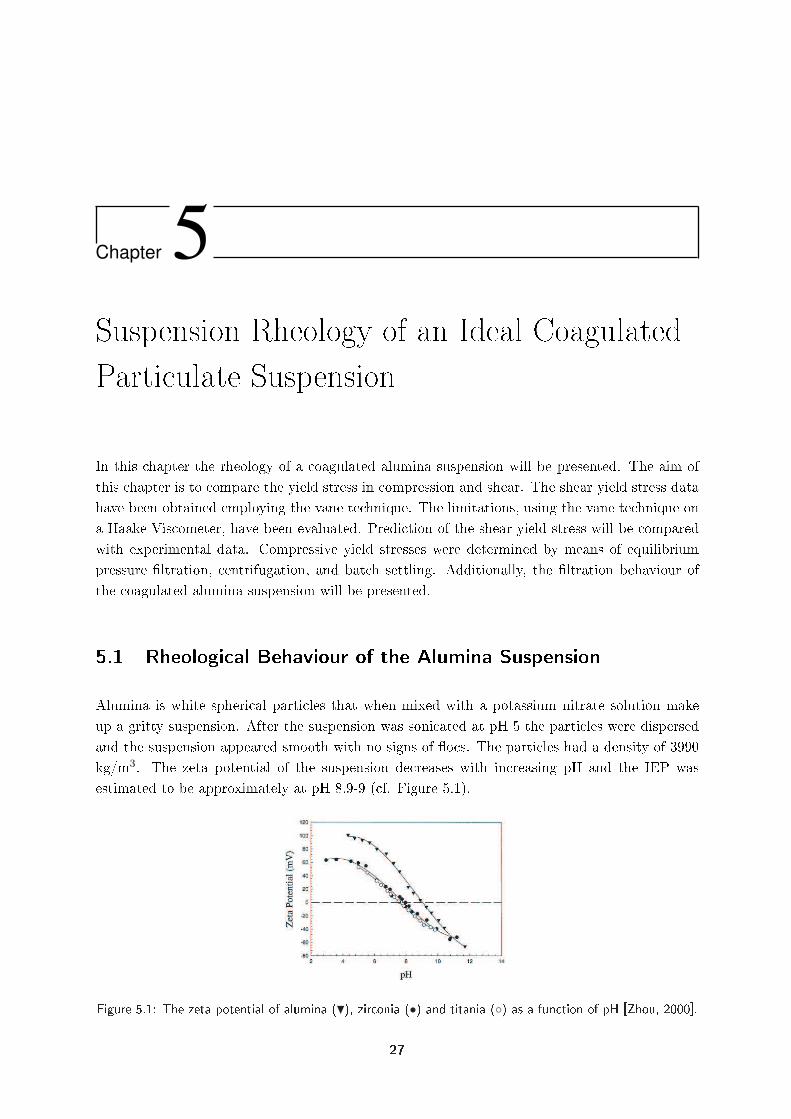
Alumina is white spherical particles that when mixed with a potassium nitrate solution makeup a gritty suspension. After the suspension was sonicated at pH 5 the particles were dispersedand the suspension appeared smooth with no signs of ocs. The particles had a density of 3990kg/m3. The zeta potential of the suspension decreases with increasing pH and the IEP wasestimated to be approximately at pH 8.9-9 (cf. Figure 5.1).
Figure 5.1: The zeta potential of alumina (L), zirconia (•) and titania () as a function of pH [Zhou, 2000].
27
Chapter 5. Suspension Rheology of an Ideal Coagulated Particulate Suspension
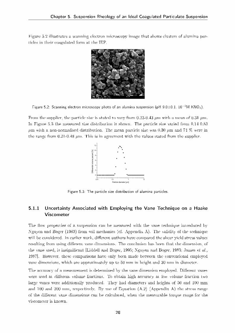
Figure 5.2 illustrates a scanning electron microscopy image that shows clusters of alumina par-ticles in their coagulated form at the IEP.
Figure 5.2: Scanning electron microscopy photo of an alumina suspension (pH 9.0±0.1, 10−2M KNO3).
From the supplier, the particle size is stated to vary from 0.23-0.43 µm with a mean of 0.31 µm.In Figure 5.3 the measured size distribution is shown. The particle size varied from 0.14-0.83µm with a non-normalised distribution. The mean particle size was 0.30 µm and 74 % were inthe range from 0.21-0.48 µm. This is in agreement with the values stated from the supplier.
0.01 0.1 1 10
0
2
4
6
8
10
12
Diff
ere
ntia
l volu
me p
erc
ent [%
]
Particle diameter [µm]
Figure 5.3: The particle size distribution of alumina particles.
5.1.1 Uncertainty Associated with Employing the Vane Technique on a HaakeViscometer
The ow properties of a suspension can be measured with the vane technique introduced byNguyen and Boger (1983) from soil mechanics (cf. Appendix A). The validity of the techniquewill be considered. In earlier work, dierent authors have compared the shear yield stress valuesresulting from using dierent vane dimensions. The conclusion has been that the dimension, ofthe vane used, is insignicant [Liddell and Boger, 1995; Nguyen and Boger, 1983; James et al.,1987]. However, these comparisons have only been made between the conventional employedvane dimensions, which are approximately up to 50 mm in height and 30 mm in diameter.The accuracy of a measurement is determined by the vane dimension employed. Dierent vaneswere used at dierent volume fractions. To obtain high accuracy at low volume fraction twolarge vanes were additionally produced. They had diameters and heights of 50 and 100 mmand 100 and 200 mm, respectively. By use of Equation (A.2) (Appendix A) the stress rangeof the dierent vane dimensions can be calculated, when the measurable torque range for theviscometer is known.
28
5.1 Rheological Behaviour of the Alumina Suspension
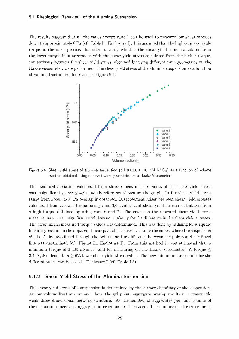
The results suggest that all the vanes except vane 1 can be used to measure low shear stressesdown to approximately 6 Pa (cf. Table I.1 Enclosure I). It is assumed that the highest measurabletorque is the most precise. In order to verify whether the shear yield stress calculated fromthe lower torque is in agreement with the shear yield stress calculated from the higher torque,comparisons between the shear yield stress, obtained by using dierent vane geometries on theHaake viscometer, were performed. The shear yield stress of the alumina suspension as a functionof volume fraction is illustrated in Figure 5.4.
0.00 0.05 0.10 0.15 0.20 0.25 0.30 0.35
1E-3
0.01
0.1
1
Shear yi
eld
stress
[kP
a]
Volume fraction [-]
vane 2 vane 3 vane 4 vane 5 vane 6 vane 7
Figure 5.4: Shear yield stress of alumina suspension (pH 9.0±0.1, 10−2M KNO3) as a function of volumefraction obtained using dierent vane geometries on a Haake Viscometer.
The standard deviation calculated from three repeat measurements of the shear yield stresswas insignicant (error ≤ 4%) and therefore not shown on the graph. In the shear yield stressrange from about 4-50 Pa overlap is observed. Disagreement arises between shear yield stressescalculated from a lower torque using vane 3,4, and 5, and shear yield stresses calculated froma high torque obtained by using vane 6 and 7. The error, on the repeated shear yield stressmeasurement, was insignicant and does not make up for the dierence in the shear yield stresses.The error on the measured torque values was determined. This was done by utilising least squarelinear regression on the apparent linear part of the stress vs. time the curve, where the suspensionyields. A line was tted through the points and the dierence between the points and the ttedline was determined (cf. Figure I.1 Enclosure I). From this method it was estimated that aminimum torque of 3,400 µNm is valid for measuring on the Haake Viscometer. A torque ≤3,400 µNm leads to a ≥ 6% lower shear yield stress value. The new minimum stress limit for thedierent vanes can be seen in Enclosure I (cf. Table I.3).
5.1.2 Shear Yield Stress of the Alumina Suspension
The shear yield stress of a suspension is determined by the surface chemistry of the suspension.At low volume fractions, at and above the gel point, aggregate overlap results in a reasonableweak three dimensional network structure. As the number of aggregates per unit volume ofthe suspension increases, aggregate interactions are increased. The number of attractive forces
29
Chapter 5. Suspension Rheology of an Ideal Coagulated Particulate Suspension
per unit volume of the suspension is increased and thus the force required to break down thisnetwork. An ideal suspension, is expected to form a crystal-like close packing structure near themaximum packing fraction. Based on these expectations, the strength of the three dimensionalnetwork structure formed in a suspension is expected to increase with an increasing rate as thevolume fraction increases.Based on knowledge of the surface chemistry of a suspension Kapur et al. (1997) proposed atheoretical model which was further modied by Scales et al. (1998). At the IEP, where therepulsive electrostatic forces are non-existent, the model can be reduced to Equation (5.1) andcan be used to predict the shear yield stress of the alumina suspension.
τy = 0.011 · AφK(φ)πD2d
(5.1)
where A is the Hamaker constant, D is the particle separation distance, d is the diameter of theparticles, and K(φ) is the mean coordination number which can be expressed by the Gotoh'sequation cited by Suzuki et al. (1981):
K(φ) =36π
φ, φ ≤ 0.47 (5.2)
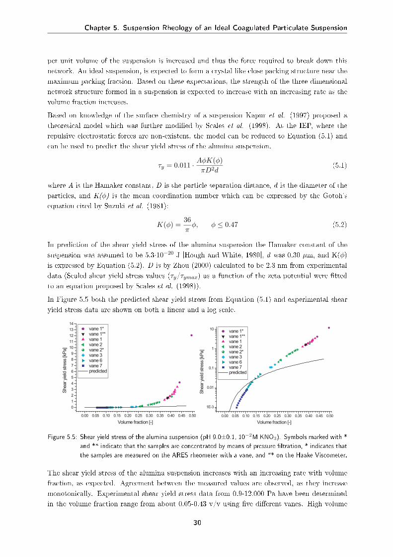
In prediction of the shear yield stress of the alumina suspension the Hamaker constant of thesuspension was assumed to be 5.3·10−20 J [Hough and White, 1980], d was 0.30 µm, and K(φ)is expressed by Equation (5.2). D is by Zhou (2000) calculated to be 2.3 nm from experimentaldata (Scaled shear yield stress values (τy/τymax) as a function of the zeta potential were ttedto an equation proposed by Scales et al. (1998)).In Figure 5.5 both the predicted shear yield stress from Equation (5.1) and experimental shearyield stress data are shown on both a linear and a log scale.
0.00 0.05 0.10 0.15 0.20 0.25 0.30 0.35 0.40 0.45 0.50
0
1
2
3
4
5
6
7
8
9
10
11
12
13
14
Shear yi
eld
stress
[kP
a]
Volume fraction [-]
vane 1* vane 1** vane 1 vane 2 vane 2* vane 3 vane 6 vane 7 predicted
0.00 0.05 0.10 0.15 0.20 0.25 0.30 0.35 0.40 0.45 0.50
1E-3
0.01
0.1
1
10
Shear yi
eld
stress
[kP
a]
Volume fraction [-]
vane 1* vane 1** vane 1 vane 2 vane 2* vane 3 vane 6 vane 7 predicted
Figure 5.5: Shear yield stress of the alumina suspension (pH 9.0±0.1, 10−2M KNO3). Symbols marked with *and ** indicate that the samples are concentrated by means of pressure ltration, * indicates thatthe samples are measured on the ARES rheometer with a vane, and ** on the Haake Viscometer.
The shear yield stress of the alumina suspension increases with an increasing rate with volumefraction, as expected. Agreement between the measured values are observed, as they increasemonotonically. Experimental shear yield stress data from 0.9-12,000 Pa have been determinedin the volume fraction range from about 0.05-0.43 v/v using ve dierent vanes. High volume
30
5.1 Rheological Behaviour of the Alumina Suspension
fractions were obtained by ltration and the corresponding shear yield stresses were measuredon either Haake Viscometer or the ARES rheometer. The dierent vane dimensions, measureequipments, and methods for concentrating the suspensions do not seem to aect the shear yieldstress measurements, as overlaps of the measured shear yield stress values are observed.
The predicted shear yield stress is not in agreement with the experimental shear yield stressvalues. At low volume fractions < 0.10 v/v, the predicted shear yield stress is too high. Abovea volume fraction of 0.10 v/v the predicted shear yield stress is too low. It appears that thepredicted shear yield stress does not account for the rapid increase in particle interactions withvolume fraction. Choose of coordination number will have an inuence on the predicted shearyield stress, as this predicts the increase of aggregate interactions, as the volume fraction in-creases.
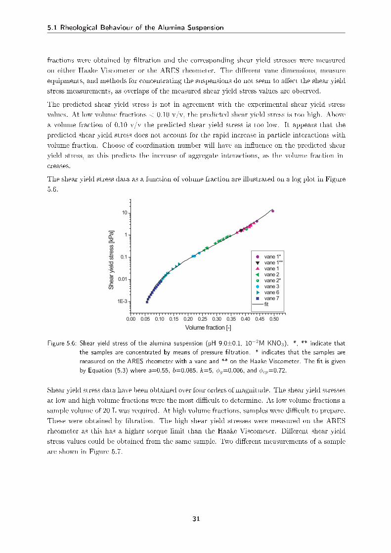
The shear yield stress data as a function of volume fraction are illustrated on a log plot in Figure5.6.
0.00 0.05 0.10 0.15 0.20 0.25 0.30 0.35 0.40 0.45 0.50
1E-3
0.01
0.1
1
10
Shear yi
eld
stress
[kP
a]
Volume fraction [-]
vane 1* vane 1** vane 1 vane 2 vane 2* vane 3 vane 6 vane 7 fit
Figure 5.6: Shear yield stress of the alumina suspension (pH 9.0±0.1, 10−2M KNO3). *, ** indicate thatthe samples are concentrated by means of pressure ltration. * indicates that the samples aremeasured on the ARES rheometer with a vane and ** on the Haake Viscometer. The t is givenby Equation (5.3) where a=0.55, b=0.085, k=5, φg=0.006, and φcp=0.72.
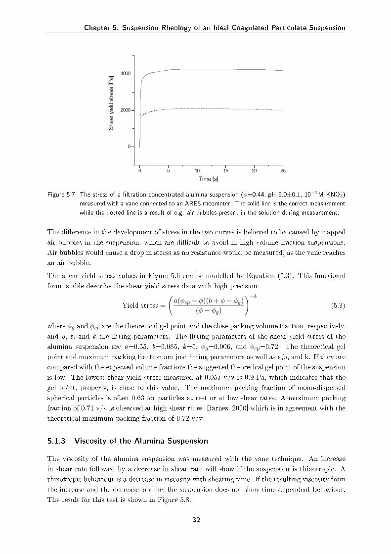
Shear yield stress data have been obtained over four orders of magnitude. The shear yield stressesat low and high volume fractions were the most dicult to determine. At low volume fractions asample volume of 20 L was required. At high volume fractions, samples were dicult to prepare.These were obtained by ltration. The high shear yield stresses were measured on the ARESrheometer as this has a higher torque limit than the Haake Viscometer. Dierent shear yieldstress values could be obtained from the same sample. Two dierent measurements of a sampleare shown in Figure 5.7.
31
Chapter 5. Suspension Rheology of an Ideal Coagulated Particulate Suspension
0 5 10 15 20 25
0
2000
4000
Shear yi
eld
stress
[P
a]
Time [s]
Figure 5.7: The stress of a ltration concentrated alumina suspension (φ=0.44, pH 9.0±0.1, 10−2M KNO3)measured with a vane connected to an ARES rheometer. The solid line is the correct measurementwhile the dotted line is a result of e.g. air bubbles present in the solution during measurement.
The dierence in the development of stress in the two curves is believed to be caused by trappedair bubbles in the suspension, which are dicult to avoid in high volume fraction suspensions.Air bubbles would cause a drop in stress as no resistance would be measured, as the vane reachesan air bubble.The shear yield stress values in Figure 5.6 can be modelled by Equation (5.3). This functionalform is able describe the shear yield stress data with high precision.
Yield stress =
(a(φcp − φ)(b + φ− φg)
(φ− φg)
)−k
(5.3)
where φg and φcp are the theoretical gel point and the close packing volume fraction, respectively,and a, b, and k are tting parameters. The tting parameters of the shear yield stress of thealumina suspension are a=0.55, b=0.085, k=5, φg=0.006, and φcp=0.72. The theoretical gelpoint and maximum packing fraction are just tting parameters as well as a,b, and k. If they arecompared with the expected volume fractions the suggested theoretical gel point of the suspensionis low. The lowest shear yield stress measured at 0.057 v/v is 0.9 Pa, which indicates that thegel point, properly, is close to this value. The maximum packing fraction of mono-dispersedspherical particles is often 0.63 for particles at rest or at low shear rates. A maximum packingfraction of 0.71 v/v is observed at high shear rates [Barnes, 2000] which is in agreement with thetheoretical maximum packing fraction of 0.72 v/v.
5.1.3 Viscosity of the Alumina Suspension
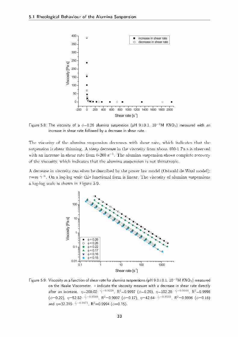
The viscosity of the alumina suspension was measured with the vane technique. An increasein shear rate followed by a decrease in shear rate will show if the suspension is thixotropic. Athixotropic behaviour is a decrease in viscosity with shearing time. If the resulting viscosity fromthe increase and the decrease is alike, the suspension does not show time dependent behaviour.The result for this test is shown in Figure 5.8.
32
5.1 Rheological Behaviour of the Alumina Suspension
-200 0 200 400 600 800 1000 1200 1400 1600 1800 2000
0
50
100
150
200
250
300
350
400 increase in shear rate decrease in shear rate
Vis
cosi
ty [P
a s
]
Shear rate [s-1]
Figure 5.8: The viscosity of a φ=0.26 alumina suspension (pH 9±0.1, 10−2M KNO3) measured with anincrease in shear rate followed by a decrease in shear rate.
The viscosity of the alumina suspension decreases with shear rate, which indicates that thesuspension is shear thinning. A steep decrease in the viscosity from about 400-1 Pa s is observedwith an increase in shear rate from 0-200 s−1. The alumina suspension shows complete recoveryof the viscosity, which indicates that the alumina suspension is not thixotropic.
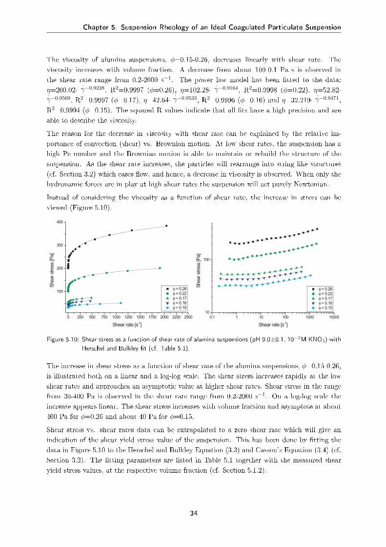
A decrease in viscosity can often be described by the power law model (Ostwald de Waal model):τ=m
·γ n. On a log-log scale this functional form is linear. The viscosity of alumina suspensions
a log-log scale is shown in Figure 5.9.
0.1 1 10 100 1000
0.01
0.1
1
10
100
Vis
cosi
ty [P
a s
]
Shear rate [s-1]
φ = 0.26 φ = 0.26 φ = 0.22 φ = 0.17 φ = 0.16 φ = 0.15
Figure 5.9: Viscosity as a function of shear rate for alumina suspensions (pH 9.0±0.1, 10−2M KNO3) measuredon the Haake Viscometer. indicate the viscosity measure with a decrease in shear rate directlyafter an increase. η=200.02· ·
γ−0.9228, R2=0.9997 (φ=0.26), η=102.28· ·γ−0.9164, R2=0.9998
(φ=0.22), η=52.82· ·γ−0.9569, R2=0.9997 (φ=0.17), η=42.64· ·
γ−0.9533, R2=0.9996 (φ=0.16)and η=32.219· ·γ−0.9471, R2=0.9994 (φ=0.15).
33
Chapter 5. Suspension Rheology of an Ideal Coagulated Particulate Suspension
The viscosity of alumina suspensions, φ=0.15-0.26, decreases linearly with shear rate. Theviscosity increases with volume fraction. A decrease from about 100-0.1 Pa s is observed inthe shear rate range from 0.2-2000 s−1. The power law model has been tted to the data:η=200.02· ·
γ−0.9228, R2=0.9997 (φ=0.26), η=102.28· ·γ−0.9164, R2=0.9998 (φ=0.22), η=52.82·
·γ−0.9569, R2=0.9997 (φ=0.17), η=42.64· ·γ−0.9533, R2=0.9996 (φ=0.16) and η=32.219· ·γ−0.9471,R2=0.9994 (φ=0.15). The squared R values indicate that all ts have a high precision and areable to describe the viscosity.
The reason for the decrease in viscosity with shear rate can be explained by the relative im-portance of convection (shear) vs. Brownian motion. At low shear rates, the suspension has ahigh Pe number and the Brownian motion is able to maintain or rebuild the structure of thesuspension. As the shear rate increases, the particles will rearrange into string like structures(cf. Section 3.2) which eases ow, and hence, a decrease in viscosity is observed. When only thehydronamic forces are in play at high shear rates the suspension will act purely Newtonian.
Instead of considering the viscosity as a function of shear rate, the increase in stress can beviewed (Figure 5.10).
0 250 500 750 1000 1250 1500 1750 2000 2250 2500
100
200
300
400
Shear st
ress
[P
a]
Shear rate [s-1]
φ = 0.26 φ = 0.22 φ = 0.17 φ = 0.16 φ = 0.15
0.1 1 10 100 1000 10000
10
100
Shear st
ress
[P
a]
Shear rate [s-1]
φ = 0.26 φ = 0.22 φ = 0.17 φ = 0.16 φ = 0.15
Figure 5.10: Shear stress as a function of shear rate of alumina suspensions (pH 9.0±0.1, 10−2M KNO3) withHerschel and Bulkley t (cf. Table 5.1).
The increase in shear stress as a function of shear rate of the alumina suspensions, φ=0.15-0.26,is illustrated both on a linear and a log-log scale. The shear stress increases rapidly at the lowshear rates and approaches an asymptotic value at higher shear rates. Shear stress in the rangefrom 30-400 Pa is observed in the shear rate range from 0.2-2000 s−1. On a log-log scale theincrease appears linear. The shear stress increases with volume fraction and asymptote at about400 Pa for φ=0.26 and about 40 Pa for φ=0.15.
Shear stress vs. shear rates data can be extrapolated to a zero shear rate which will give anindication of the shear yield stress value of the suspension. This has been done by tting thedata in Figure 5.10 to the Herschel and Bulkley Equation (3.3) and Casson's Equation (3.4) (cf.Section 3.2). The tting parameters are listed in Table 5.1 together with the measured shearyield stress values, at the respective volume fraction (cf. Section 5.1.2).
34
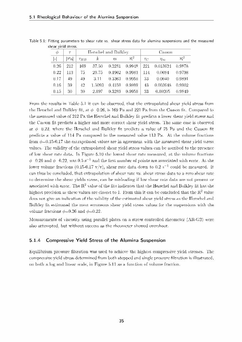
5.1 Rheological Behaviour of the Alumina Suspension
Table 5.1: Fitting parameters to shear rate vs. shear stress data for alumina suspensions and the measuredshear yield stress.
φ τ Herschel and Bulkley Casson[-] [Pa] τHB k m R2 τC η∞ R2
0.26 212 169 37.50 0.2281 0.9948 221 0.013624 0.98780.22 113 75 29.75 0.1902 0.9983 114 0.0084 0.97980.17 49 49 3.11 0.3363 0.9950 53 0.0040 0.98910.16 39 42 1.5093 0.4150 0.9899 43 0.003648 0.99020.15 30 30 2.097 0.3289 0.9950 33 0.00205 0.9849
From the results in Table 5.1 it can be observed, that the extrapolated shear yield stress fromthe Herschel and Bulkley t, at φ=0.26, is 169 Pa and 221 Pa from the Casson t. Compared tothe measured value of 212 Pa the Herschel and Bulkley t predicts a lower shear yield stress andthe Casson t predicts a higher and more correct shear yield stress. The same case is observedat φ=0.22, where the Herschel and Bulkley t predicts a value of 75 Pa and the Casson tpredicts a value of 114 Pa compared to the measured value 113 Pa. At the volume fractionsfrom φ=0.15-0.17 the extrapolated values are in agreement with the measured shear yield stressvalues. The validity of the extrapolated shear yield stress values can be ascribed to the presenceof low shear rate data. In Figure 5.10 the lowest shear rate measured, at the volume fractionsφ=0.26 and φ=0.22, was 0.5 s−1 and the rst number of points are associated with error. At thelower volume fractions (0.15-0.17 v/v), shear rate data down to 0.2 s−1 could be measured. Itcan thus be concluded, that extrapolation of shear rate vs. shear stress data to a zero shear rateto determine the shear yields stress, can be misleading if low shear rate data are not present orassociated with error. The R2 value of the ts indicates that the Herschel and Bulkley t has thehighest precision as these values are closest to 1. From this it can be concluded that the R2 valuedoes not give an indication of the validity of the estimated shear yield stress as the Herschel andBulkley t estimated the most erroneous shear yield stress values for the suspensions with thevolume fractions φ=0.26 and φ=0.22.
Measurements of viscosity using parallel plates on a stress controlled rheometer (AR-G2) werealso attempted, but without success as the rheometer showed overshoot.
5.1.4 Compressive Yield Stress of the Alumina Suspension
Equilibrium pressure ltration was used to achieve the highest compressive yield stresses. Thecompressive yield stress determined from both stepped and single pressure ltration is illustrated,on both a log and linear scale, in Figure 5.11 as a function of volume fraction.
35
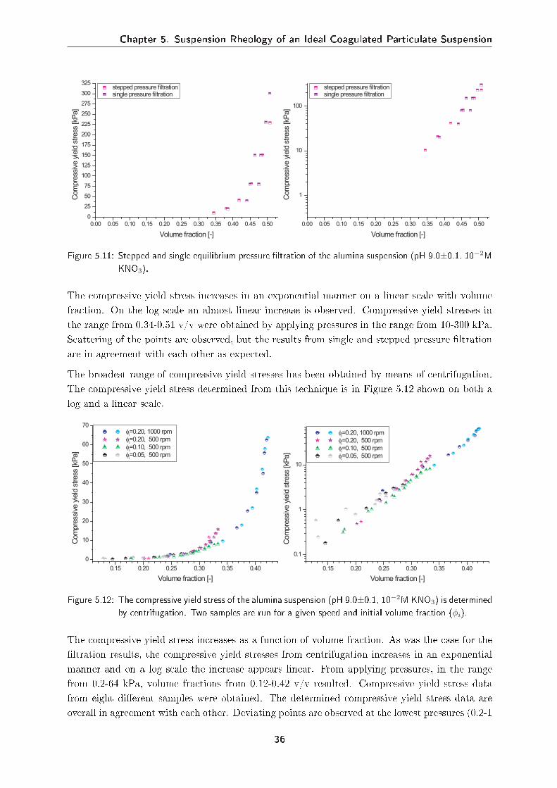
Chapter 5. Suspension Rheology of an Ideal Coagulated Particulate Suspension
0.00 0.05 0.10 0.15 0.20 0.25 0.30 0.35 0.40 0.45 0.50
0
25
50
75
100
125
150
175
200
225
250
275
300
325
Com
pre
ssiv
e y
ield
stress
[kP
a]
Volume fraction [-]
stepped pressure filtration single pressure filtration
0.00 0.05 0.10 0.15 0.20 0.25 0.30 0.35 0.40 0.45 0.50
1
10
100
Com
pre
ssiv
e y
ield
stress
[kP
a]
Volume fraction [-]
stepped pressure filtration single pressure filtration
Figure 5.11: Stepped and single equilibrium pressure ltration of the alumina suspension (pH 9.0±0.1, 10−2MKNO3).
The compressive yield stress increases in an exponential manner on a linear scale with volumefraction. On the log scale an almost linear increase is observed. Compressive yield stresses inthe range from 0.34-0.51 v/v were obtained by applying pressures in the range from 10-300 kPa.Scattering of the points are observed, but the results from single and stepped pressure ltrationare in agreement with each other as expected.
The broadest range of compressive yield stresses has been obtained by means of centrifugation.The compressive yield stress determined from this technique is in Figure 5.12 shown on both alog and a linear scale.
0.15 0.20 0.25 0.30 0.35 0.40
0
10
20
30
40
50
60
70 φ
i=0.20, 1000 rpm
φi=0.20, 500 rpm
φi=0.10, 500 rpm
φi=0.05, 500 rpm
Com
pre
ssiv
e y
ield
stress
[kP
a]
Volume fraction [-]
0.15 0.20 0.25 0.30 0.35 0.40
0.1
1
10
φi=0.20, 1000 rpm
φi=0.20, 500 rpm
φi=0.10, 500 rpm
φi=0.05, 500 rpm
Com
pre
ssiv
e y
ield
stress
[kP
a]
Volume fraction [-]
Figure 5.12: The compressive yield stress of the alumina suspension (pH 9.0±0.1, 10−2M KNO3) is determinedby centrifugation. Two samples are run for a given speed and initial volume fraction (φi).
The compressive yield stress increases as a function of volume fraction. As was the case for theltration results, the compressive yield stresses from centrifugation increases in an exponentialmanner and on a log scale the increase appears linear. From applying pressures, in the rangefrom 0.2-64 kPa, volume fractions from 0.12-0.42 v/v resulted. Compressive yield stress datafrom eight dierent samples were obtained. The determined compressive yield stress data areoverall in agreement with each other. Deviating points are observed at the lowest pressures (0.2-1
36
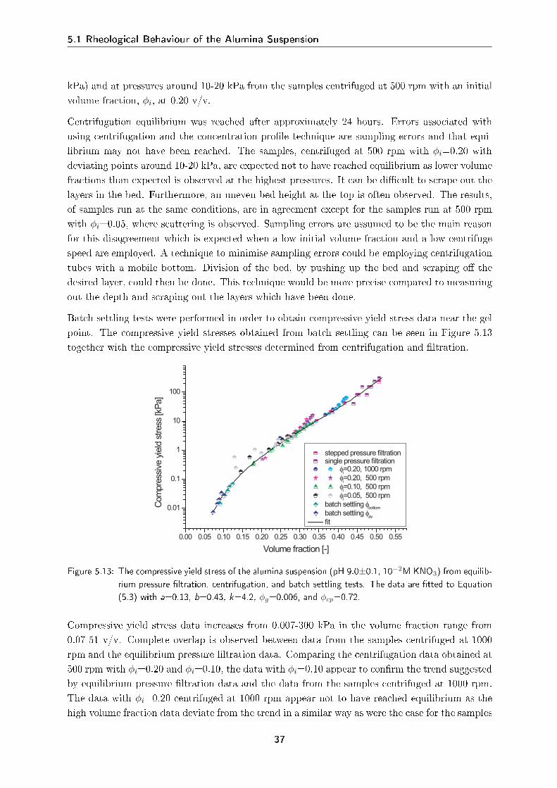
5.1 Rheological Behaviour of the Alumina Suspension
kPa) and at pressures around 10-20 kPa from the samples centrifuged at 500 rpm with an initialvolume fraction, φi, at 0.20 v/v.
Centrifugation equilibrium was reached after approximately 24 hours. Errors associated withusing centrifugation and the concentration prole technique are sampling errors and that equi-librium may not have been reached. The samples, centrifuged at 500 rpm with φi=0.20 withdeviating points around 10-20 kPa, are expected not to have reached equilibrium as lower volumefractions than expected is observed at the highest pressures. It can be dicult to scrape out thelayers in the bed. Furthermore, an uneven bed height at the top is often observed. The results,of samples run at the same conditions, are in agreement except for the samples run at 500 rpmwith φi=0.05, where scattering is observed. Sampling errors are assumed to be the main reasonfor this disagreement which is expected when a low initial volume fraction and a low centrifugespeed are employed. A technique to minimise sampling errors could be employing centrifugationtubes with a mobile bottom. Division of the bed, by pushing up the bed and scraping o thedesired layer, could then be done. This technique would be more precise compared to measuringout the depth and scraping out the layers which have been done.
Batch settling tests were performed in order to obtain compressive yield stress data near the gelpoint. The compressive yield stresses obtained from batch settling can be seen in Figure 5.13together with the compressive yield stresses determined from centrifugation and ltration.
0.00 0.05 0.10 0.15 0.20 0.25 0.30 0.35 0.40 0.45 0.50 0.55
0.01
0.1
1
10
100
stepped pressure filtration single pressure filtration
φi=0.20, 1000 rpm
φi=0.20, 500 rpm
φi=0.10, 500 rpm
φi=0.05, 500 rpm
batch settling φbottom
batch settling φav
fit
Com
pre
ssiv
e y
ield
stress
[kP
a]
Volume fraction [-]
Figure 5.13: The compressive yield stress of the alumina suspension (pH 9.0±0.1, 10−2M KNO3) from equilib-rium pressure ltration, centrifugation, and batch settling tests. The data are tted to Equation(5.3) with a=0.13, b=0.43, k=4.2, φg=0.006, and φcp=0.72.
Compressive yield stress data increases from 0.007-300 kPa in the volume fraction range from0.07-51 v/v. Complete overlap is observed between data from the samples centrifuged at 1000rpm and the equilibrium pressure ltration data. Comparing the centrifugation data obtained at500 rpm with φi=0.20 and φi=0.10, the data with φi=0.10 appear to conrm the trend suggestedby equilibrium pressure ltration data and the data from the samples centrifuged at 1000 rpm.The data with φi=0.20 centrifuged at 1000 rpm appear not to have reached equilibrium as thehigh volume fraction data deviate from the trend in a similar way as were the case for the samples
37
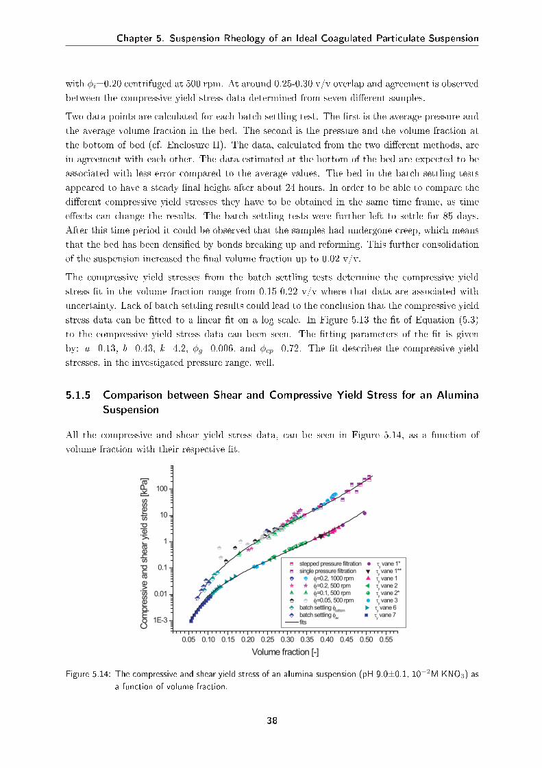
Chapter 5. Suspension Rheology of an Ideal Coagulated Particulate Suspension
with φi=0.20 centrifuged at 500 rpm. At around 0.25-0.30 v/v overlap and agreement is observedbetween the compressive yield stress data determined from seven dierent samples.
Two data points are calculated for each batch settling test. The rst is the average pressure andthe average volume fraction in the bed. The second is the pressure and the volume fraction atthe bottom of bed (cf. Enclosure II). The data, calculated from the two dierent methods, arein agreement with each other. The data estimated at the bottom of the bed are expected to beassociated with less error compared to the average values. The bed in the batch settling testsappeared to have a steady nal height after about 24 hours. In order to be able to compare thedierent compressive yield stresses they have to be obtained in the same time frame, as timeeects can change the results. The batch settling tests were further left to settle for 85 days.After this time period it could be observed that the samples had undergone creep, which meansthat the bed has been densied by bonds breaking up and reforming. This further consolidationof the suspension increased the nal volume fraction up to 0.02 v/v.
The compressive yield stresses from the batch settling tests determine the compressive yieldstress t in the volume fraction range from 0.15-0.22 v/v where that data are associated withuncertainty. Lack of batch settling results could lead to the conclusion that the compressive yieldstress data can be tted to a linear t on a log scale. In Figure 5.13 the t of Equation (5.3)to the compressive yield stress data can been seen. The tting parameters of the t is givenby: a=0.13, b=0.43, k=4.2, φg=0.006, and φcp=0.72. The t describes the compressive yieldstresses, in the investigated pressure range, well.
5.1.5 Comparison between Shear and Compressive Yield Stress for an AluminaSuspension
All the compressive and shear yield stress data, can be seen in Figure 5.14, as a function ofvolume fraction with their respective t.
0.05 0.10 0.15 0.20 0.25 0.30 0.35 0.40 0.45 0.50 0.55
1E-3
0.01
0.1
1
10
100
stepped pressure filtration τy vane 1*
single pressure filtration τy vane 1**
φi=0.2, 1000 rpm τ
y vane 1
φi=0.2, 500 rpm τ
y vane 2
φi=0.1, 500 rpm τ
y vane 2*
φi=0.05, 500 rpm τ
y vane 3
batch settling φbottom
τy vane 6
batch settling φav τ
y vane 7
fits
Com
pre
ssiv
e a
nd s
hear yi
eld
stress
[kP
a]
Volume fraction [-]
Figure 5.14: The compressive and shear yield stress of an alumina suspension (pH 9.0±0.1, 10−2M KNO3) asa function of volume fraction.
38
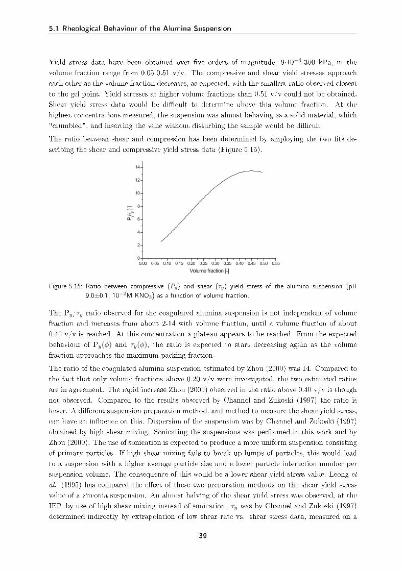
5.1 Rheological Behaviour of the Alumina Suspension
Yield stress data have been obtained over ve orders of magnitude, 9·10−4-300 kPa, in thevolume fraction range from 0.05-0.51 v/v. The compressive and shear yield stresses approacheach other as the volume fraction decreases, as expected, with the smallest ratio observed closestto the gel point. Yield stresses at higher volume fractions than 0.51 v/v could not be obtained.Shear yield stress data would be dicult to determine above this volume fraction. At thehighest concentrations measured, the suspension was almost behaving as a solid material, which"crumbled", and inserting the vane without disturbing the sample would be dicult.The ratio between shear and compression has been determined by employing the two ts de-scribing the shear and compressive yield stress data (Figure 5.15).
0.00 0.05 0.10 0.15 0.20 0.25 0.30 0.35 0.40 0.45 0.50 0.55
0
2
4
6
8
10
12
14
Py/τ
y [-]
Volume fraction [-]
Figure 5.15: Ratio between compressive (Py) and shear (τy) yield stress of the alumina suspension (pH9.0±0.1, 10−2M KNO3) as a function of volume fraction.
The Py/τy ratio observed for the coagulated alumina suspension is not independent of volumefraction and increases from about 2-14 with volume fraction, until a volume fraction of about0.40 v/v is reached. At this concentration a plateau appears to be reached. From the expectedbehaviour of Py(φ) and τy(φ), the ratio is expected to start decreasing again as the volumefraction approaches the maximum packing fraction.The ratio of the coagulated alumina suspension estimated by Zhou (2000) was 14. Compared tothe fact that only volume fractions above 0.20 v/v were investigated, the two estimated ratiosare in agreement. The rapid increase Zhou (2000) observed in the ratio above 0.40 v/v is thoughnot observed. Compared to the results observed by Channel and Zukoski (1997) the ratio islower. A dierent suspension preparation method, and method to measure the shear yield stress,can have an inuence on this. Dispersion of the suspension was by Channel and Zukoski (1997)obtained by high shear mixing. Sonicating the suspensions was performed in this work and byZhou (2000). The use of sonication is expected to produce a more uniform suspension consistingof primary particles. If high shear mixing fails to break up lumps of particles, this would leadto a suspension with a higher average particle size and a lower particle interaction number persuspension volume. The consequence of this would be a lower shear yield stress value. Leong etal. (1995) has compared the eect of these two preparation methods on the shear yield stressvalue of a zirconia suspension. An almost halving of the shear yield stress was observed, at theIEP, by use of high shear mixing instead of sonication. τy was by Channel and Zukoski (1997)determined indirectly by extrapolation of low shear rate vs. shear stress data, measured on a
39
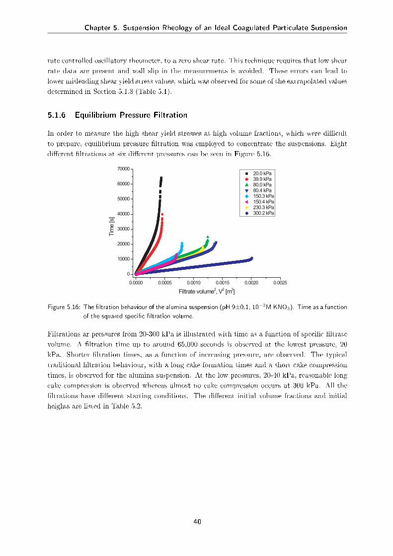
Chapter 5. Suspension Rheology of an Ideal Coagulated Particulate Suspension
rate controlled oscillatory rheometer, to a zero shear rate. This technique requires that low shearrate data are present and wall slip in the measurements is avoided. These errors can lead tolower misleading shear yield stress values, which was observed for some of the extrapolated valuesdetermined in Section 5.1.3 (Table 5.1).
5.1.6 Equilibrium Pressure Filtration
In order to measure the high shear yield stresses at high volume fractions, which were dicultto prepare, equilibrium pressure ltration was employed to concentrate the suspensions. Eightdierent ltrations at six dierent pressures can be seen in Figure 5.16.
0.0000 0.0005 0.0010 0.0015 0.0020 0.0025
0
10000
20000
30000
40000
50000
60000
70000
Tim
e [s]
Filtrate volume2, V
2 [m
2]
20.0 kPa 39.9 kPa 80.0 kPa 80.4 kPa 150.3 kPa 150.4 kPa 230.3 kPa 300.2 kPa
Figure 5.16: The ltration behaviour of the alumina suspension (pH 9±0.1, 10−2MKNO3). Time as a functionof the squared specic ltration volume.
Filtrations ar pressures from 20-300 kPa is illustrated with time as a function of specic ltratevolume. A ltration time up to around 65,000 seconds is observed at the lowest pressure, 20kPa. Shorter ltration times, as a function of increasing pressure, are observed. The typicaltraditional ltration behaviour, with a long cake formation times and a short cake compressiontimes, is observed for the alumina suspension. At the low pressures, 20-40 kPa, reasonable longcake compression is observed whereas almost no cake compression occurs at 300 kPa. All theltrations have dierent starting conditions. The dierent initial volume fractions and initialheights are listed in Table 5.2.
40
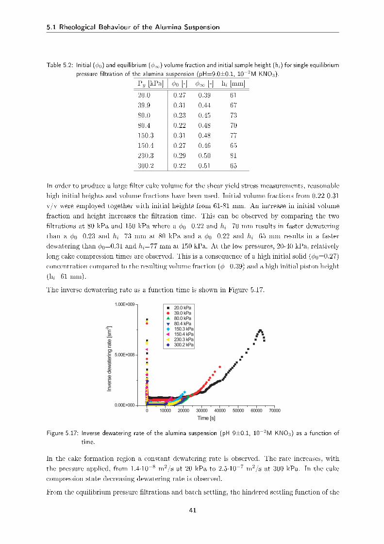
5.1 Rheological Behaviour of the Alumina Suspension
Table 5.2: Initial (φ0) and equilibrium (φ∞) volume fraction and initial sample height (hi) for single equilibriumpressure ltration of the alumina suspension (pH=9.0±0.1, 10−2M KNO3).
Py [kPa] φ0 [-] φ∞ [-] hi [mm]20.0 0.27 0.39 6139.9 0.31 0.44 6780.0 0.23 0.45 7380.4 0.22 0.48 70150.3 0.31 0.48 77150.4 0.27 0.46 65230.3 0.29 0.50 81300.2 0.22 0.51 65
In order to produce a large lter cake volume for the shear yield stress measurements, reasonablehigh initial heights and volume fractions have been used. Initial volume fractions from 0.22-0.31v/v were employed together with initial heights from 61-81 mm. An increase in initial volumefraction and height increases the ltration time. This can be observed by comparing the twoltrations at 80 kPa and 150 kPa where a φ0=0.22 and hi=70 mm results in faster dewateringthan a φ0=0.23 and hi=73 mm at 80 kPa and a φ0=0.22 and hi=65 mm results in a fasterdewatering than φ0=0.31 and hi=77 mm at 150 kPa. At the low pressures, 20-40 kPa, relativelylong cake compression times are observed. This is a consequence of a high initial solid (φ0=0.27)concentration compared to the resulting volume fraction (φ=0.39) and a high initial piston height(hi=61 mm).
The inverse dewatering rate as a function time is shown in Figure 5.17.
0 10000 20000 30000 40000 50000 60000 70000
0.00E+000
5.00E+008
1.00E+009
Inve
rse d
ew
ate
ring rate
[sm
-2]
Time [s]
20.0 kPa 39.0 kPa 80.0 kPa 80.4 kPa 150.3 kPa 150.4 kPa 230.3 kPa 300.2 kPa
Figure 5.17: Inverse dewatering rate of the alumina suspension (pH 9±0.1, 10−2M KNO3) as a function oftime.
In the cake formation region a constant dewatering rate is observed. The rate increases, withthe pressure applied, from 1.4·10−8 m2/s at 20 kPa to 2.5·10−7 m2/s at 300 kPa. In the cakecompression state decreasing dewatering rate is observed.
From the equilibrium pressure ltrations and batch settling, the hindered settling function of the
41
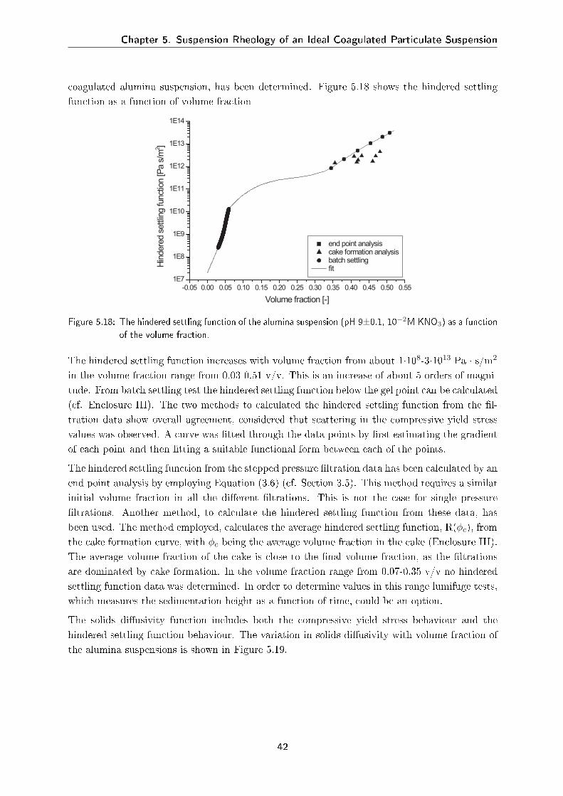
Chapter 5. Suspension Rheology of an Ideal Coagulated Particulate Suspension
coagulated alumina suspension, has been determined. Figure 5.18 shows the hindered settlingfunction as a function of volume fraction
-0.05 0.00 0.05 0.10 0.15 0.20 0.25 0.30 0.35 0.40 0.45 0.50 0.55
1E7
1E8
1E9
1E10
1E11
1E12
1E13
1E14
end point analysis cake formation analysis batch settling fit
Hin
dere
d s
ettlin
g funct
ion [P
a s
/m2 ]
Volume fraction [-]
Figure 5.18: The hindered settling function of the alumina suspension (pH 9±0.1, 10−2M KNO3) as a functionof the volume fraction.
The hindered settling function increases with volume fraction from about 1·108-3·1013 Pa · s/m2
in the volume fraction range from 0.03-0.51 v/v. This is an increase of about 5 orders of magni-tude. From batch settling test the hindered settling function below the gel point can be calculated(cf. Enclosure III). The two methods to calculated the hindered settling function from the l-tration data show overall agreement, considered that scattering in the compressive yield stressvalues was observed. A curve was tted through the data points by rst estimating the gradientof each point and then tting a suitable functional form between each of the points.
The hindered settling function from the stepped pressure ltration data has been calculated by anend point analysis by employing Equation (3.6) (cf. Section 3.5). This method requires a similarinitial volume fraction in all the dierent ltrations. This is not the case for single pressureltrations. Another method, to calculate the hindered settling function from these data, hasbeen used. The method employed, calculates the average hindered settling function, R(φc), fromthe cake formation curve, with φc being the average volume fraction in the cake (Enclosure III).The average volume fraction of the cake is close to the nal volume fraction, as the ltrationsare dominated by cake formation. In the volume fraction range from 0.07-0.35 v/v no hinderedsettling function data was determined. In order to determine values in this range lumifuge tests,which measures the sedimentation height as a function of time, could be an option.
The solids diusivity function includes both the compressive yield stress behaviour and thehindered settling function behaviour. The variation in solids diusivity with volume fraction ofthe alumina suspensions is shown in Figure 5.19.
42
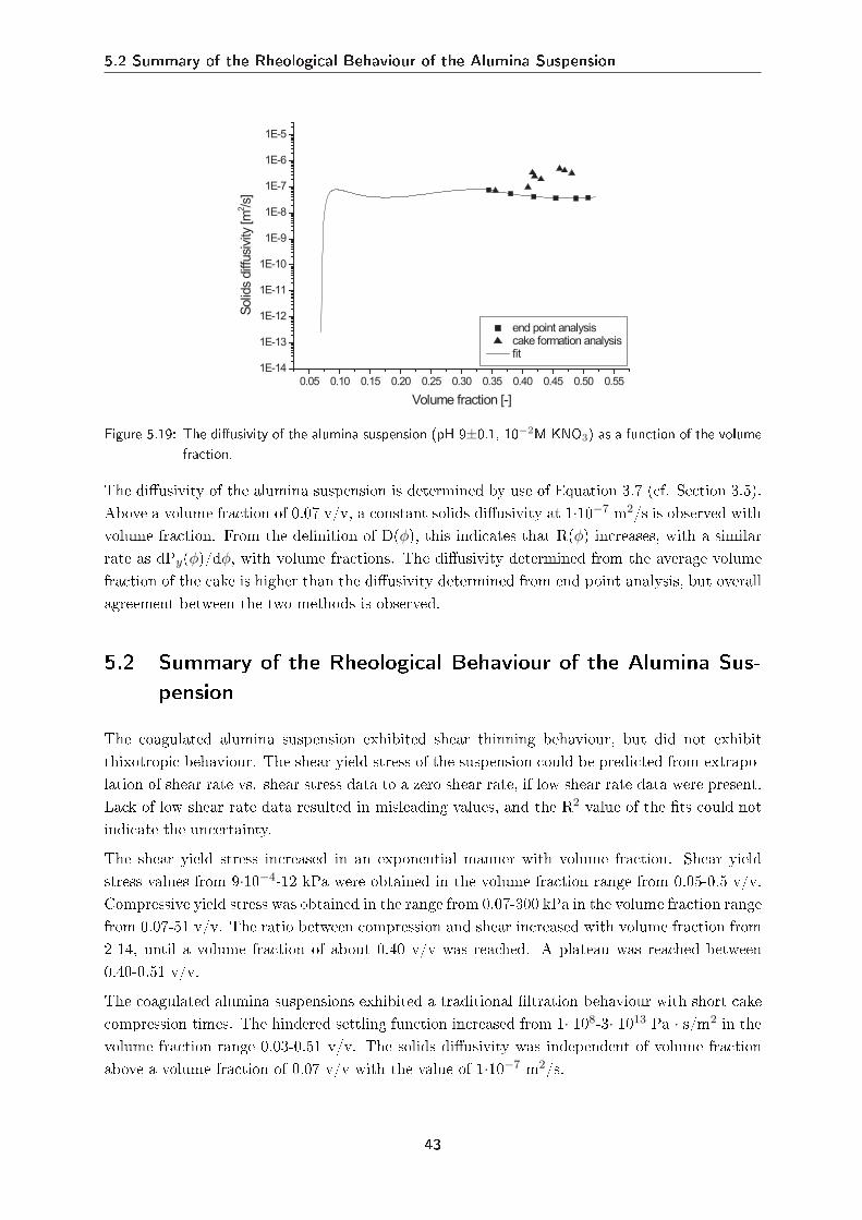
5.2 Summary of the Rheological Behaviour of the Alumina Suspension
0.05 0.10 0.15 0.20 0.25 0.30 0.35 0.40 0.45 0.50 0.55
1E-14
1E-13
1E-12
1E-11
1E-10
1E-9
1E-8
1E-7
1E-6
1E-5
end point analysis cake formation analysis fit
Solid
s diff
usi
vity
[m
2 /s]
Volume fraction [-]
Figure 5.19: The diusivity of the alumina suspension (pH 9±0.1, 10−2M KNO3) as a function of the volumefraction.
The diusivity of the alumina suspension is determined by use of Equation 3.7 (cf. Section 3.5).Above a volume fraction of 0.07 v/v, a constant solids diusivity at 1·10−7 m2/s is observed withvolume fraction. From the denition of D(φ), this indicates that R(φ) increases, with a similarrate as dPy(φ)/dφ, with volume fractions. The diusivity determined from the average volumefraction of the cake is higher than the diusivity determined from end point analysis, but overallagreement between the two methods is observed.
5.2 Summary of the Rheological Behaviour of the Alumina Sus-pension
The coagulated alumina suspension exhibited shear thinning behaviour, but did not exhibitthixotropic behaviour. The shear yield stress of the suspension could be predicted from extrapo-lation of shear rate vs. shear stress data to a zero shear rate, if low shear rate data were present.Lack of low shear rate data resulted in misleading values, and the R2 value of the ts could notindicate the uncertainty.
The shear yield stress increased in an exponential manner with volume fraction. Shear yieldstress values from 9·10−4-12 kPa were obtained in the volume fraction range from 0.05-0.5 v/v.Compressive yield stress was obtained in the range from 0.07-300 kPa in the volume fraction rangefrom 0.07-51 v/v. The ratio between compression and shear increased with volume fraction from2-14, until a volume fraction of about 0.40 v/v was reached. A plateau was reached between0.40-0.51 v/v.
The coagulated alumina suspensions exhibited a traditional ltration behaviour with short cakecompression times. The hindered settling function increased from 1· 108-3· 1013 Pa · s/m2 in thevolume fraction range 0.03-0.51 v/v. The solids diusivity was independent of volume fractionabove a volume fraction of 0.07 v/v with the value of 1·10−7 m2/s.
43

Chapter 5. Suspension Rheology of an Ideal Coagulated Particulate Suspension
44
Chapter 6Suspension Rheology of Non-Ideal ParticulateSuspensions
The scope of this chapter is to investigate the behaviour of sewage sludge and a occulatedalumina suspension in compression and shear as a function of volume fraction. In order todo this, a dual-polymer occulated alumina suspension is produced. The shear properties arecharacterised with the vane technique and the compressive properties are characterised by equi-librium pressure ltration, centrifugation, and batch settling. The ltration behaviour of the twosuspensions is presented to determine whether the suspensions exhibit non-traditional ltrationbehaviour as expected. The dual-polymer occulated alumina suspension is expected to exhibitshort ltration times compared to the sewage sludge. This would make this system ideal forfurther characterisation in the attempt to understand non-traditional ltration behaviour.
6.1 Rheological Behaviour of Sewage Sludge
In this section the rheology of sewage sludge and compression will be presented. Furthermore,characterisation of ltration behaviour and determination of ltration parameters R(φ) and D(φ)of sewage sludge will be presented.
The sewage sludge had a low initial solids concentration (φ=0.0097 v/v) and the density of theliquid and the solid was 1.0036 and 1.4715 g/cm3, respectively. The heterogeneous structure ofsewage sludge was visible by eye and a 100 times magnication is shown in Figure 6.1.
Figure 6.1: Optical microscope picture of sewage sludge, 100 times magnication.
45
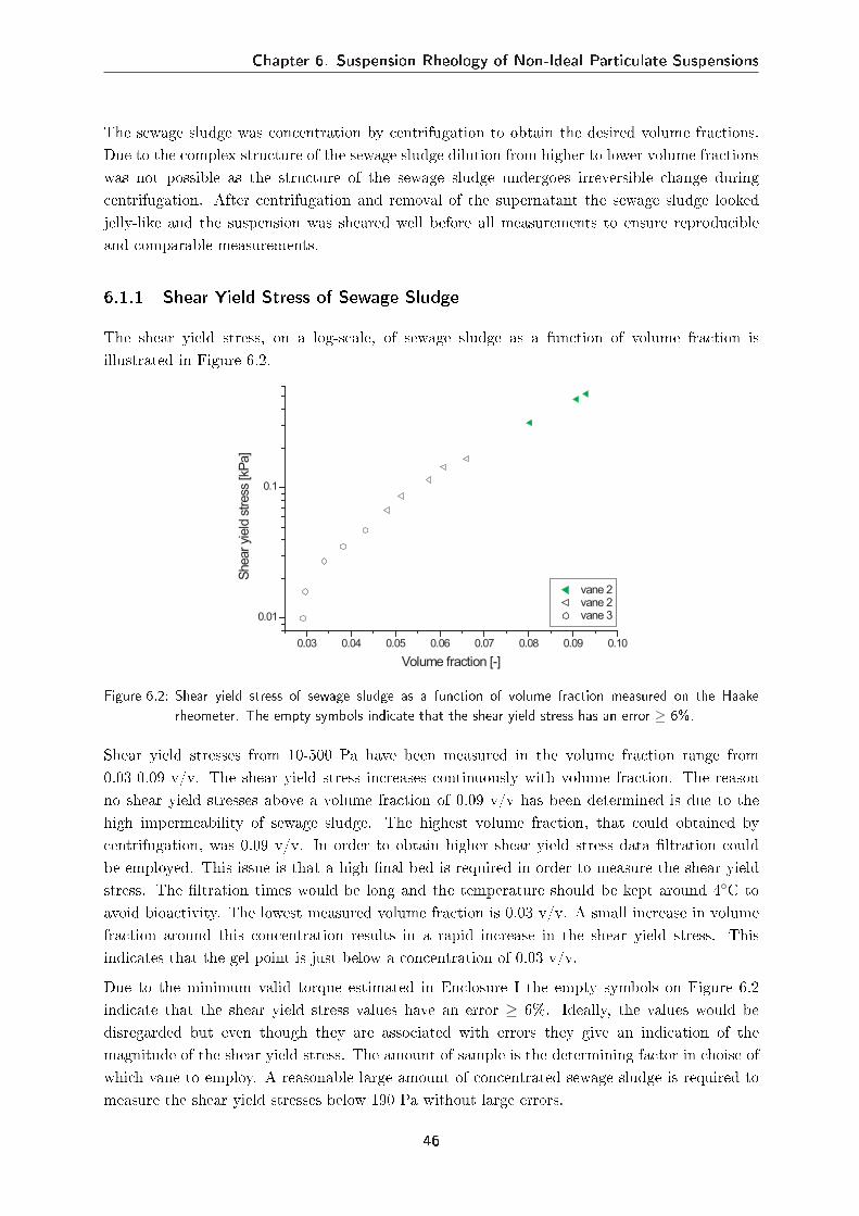
Chapter 6. Suspension Rheology of Non-Ideal Particulate Suspensions
The sewage sludge was concentration by centrifugation to obtain the desired volume fractions.Due to the complex structure of the sewage sludge dilution from higher to lower volume fractionswas not possible as the structure of the sewage sludge undergoes irreversible change duringcentrifugation. After centrifugation and removal of the supernatant the sewage sludge lookedjelly-like and the suspension was sheared well before all measurements to ensure reproducibleand comparable measurements.
6.1.1 Shear Yield Stress of Sewage Sludge
The shear yield stress, on a log-scale, of sewage sludge as a function of volume fraction isillustrated in Figure 6.2.
0.03 0.04 0.05 0.06 0.07 0.08 0.09 0.10
0.01
0.1
vane 2 vane 2 vane 3
Shear yi
eld
stress
[kP
a]
Volume fraction [-]
Figure 6.2: Shear yield stress of sewage sludge as a function of volume fraction measured on the Haakerheometer. The empty symbols indicate that the shear yield stress has an error ≥ 6%.
Shear yield stresses from 10-500 Pa have been measured in the volume fraction range from0.03-0.09 v/v. The shear yield stress increases continuously with volume fraction. The reasonno shear yield stresses above a volume fraction of 0.09 v/v has been determined is due to thehigh impermeability of sewage sludge. The highest volume fraction, that could obtained bycentrifugation, was 0.09 v/v. In order to obtain higher shear yield stress data ltration couldbe employed. This issue is that a high nal bed is required in order to measure the shear yieldstress. The ltration times would be long and the temperature should be kept around 4C toavoid bioactivity. The lowest measured volume fraction is 0.03 v/v. A small increase in volumefraction around this concentration results in a rapid increase in the shear yield stress. Thisindicates that the gel point is just below a concentration of 0.03 v/v.
Due to the minimum valid torque estimated in Enclosure I the empty symbols on Figure 6.2indicate that the shear yield stress values have an error ≥ 6%. Ideally, the values would bedisregarded but even though they are associated with errors they give an indication of themagnitude of the shear yield stress. The amount of sample is the determining factor in choise ofwhich vane to employ. A reasonable large amount of concentrated sewage sludge is required tomeasure the shear yield stresses below 190 Pa without large errors.
46
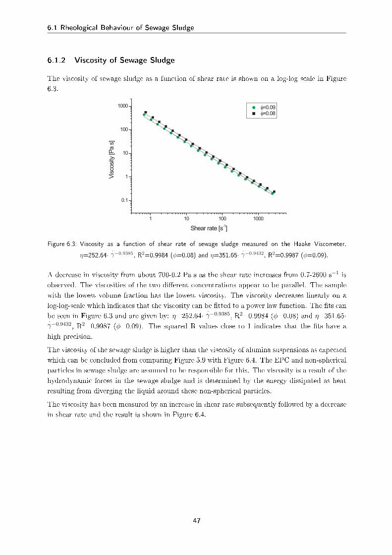
6.1 Rheological Behaviour of Sewage Sludge
6.1.2 Viscosity of Sewage Sludge
The viscosity of sewage sludge as a function of shear rate is shown on a log-log scale in Figure6.3.
1 10 100 1000
0.1
1
10
100
1000 φ=0.09 φ=0.08
Vis
cosi
ty [P
a s
]
Shear rate [s-1]
Figure 6.3: Viscosity as a function of shear rate of sewage sludge measured on the Haake Viscometer.η=252.64· ·γ−0.9385, R2=0.9984 (φ=0.08) and η=351.65· ·γ−0.9432, R2=0.9987 (φ=0.09).
A decrease in viscosity from about 700-0.2 Pa s as the shear rate increases from 0.7-2600 s−1 isobserved. The viscosities of the two dierent concentrations appear to be parallel. The samplewith the lowest volume fraction has the lowest viscosity. The viscosity decreases linearly on alog-log-scale which indicates that the viscosity can be tted to a power law function. The ts canbe seen in Figure 6.3 and are given by: η=252.64· ·γ−0.9385, R2=0.9984 (φ=0.08) and η=351.65··γ−0.9432, R2=0.9987 (φ=0.09). The squared R values close to 1 indicates that the ts have ahigh precision.
The viscosity of the sewage sludge is higher than the viscosity of alumina suspensions as expectedwhich can be concluded from comparing Figure 5.9 with Figure 6.4. The EPC and non-sphericalparticles in sewage sludge are assumed to be responsible for this. The viscosity is a result of thehydrodynamic forces in the sewage sludge and is determined by the energy dissipated as heatresulting from diverging the liquid around these non-spherical particles.
The viscosity has been measured by an increase in shear rate subsequently followed by a decreasein shear rate and the result is shown in Figure 6.4.
47
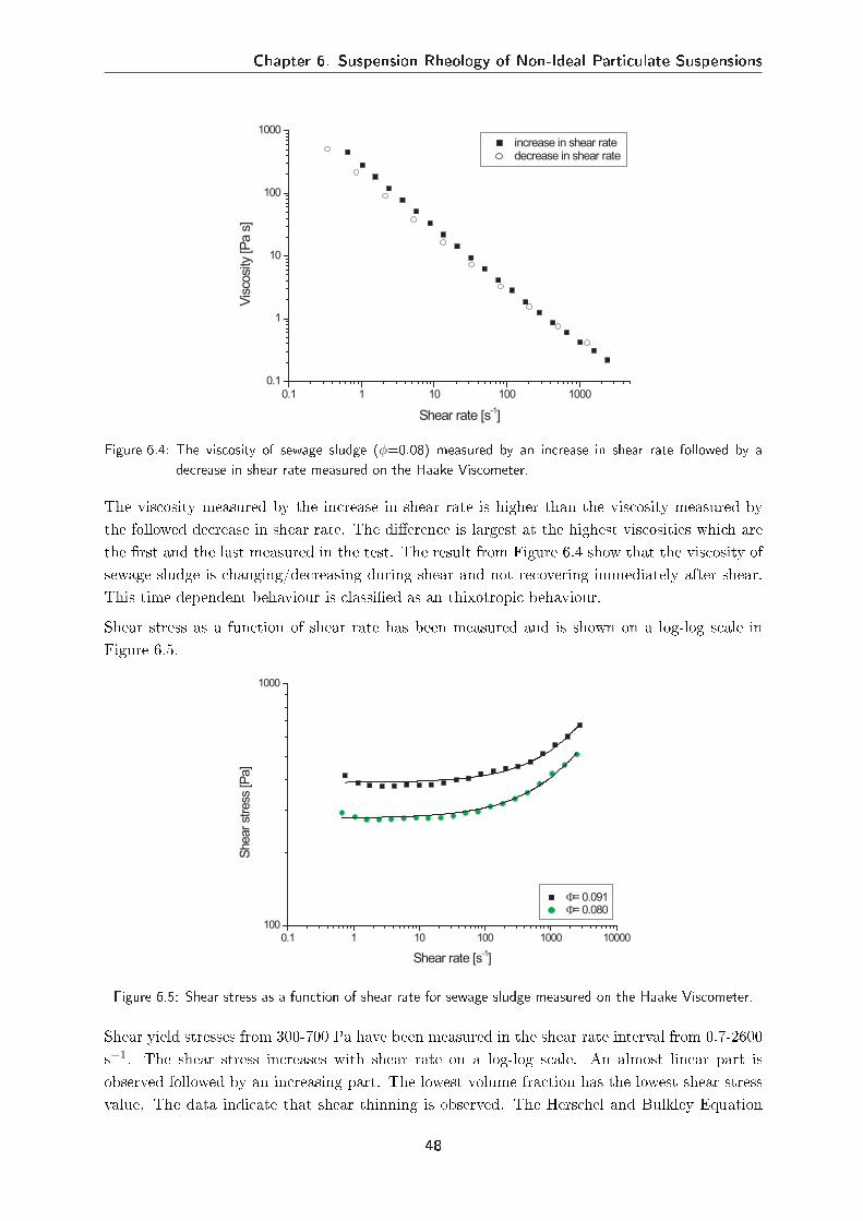
Chapter 6. Suspension Rheology of Non-Ideal Particulate Suspensions
0.1 1 10 100 1000
0.1
1
10
100
1000 increase in shear rate decrease in shear rate
Vis
cosi
ty [P
a s
]
Shear rate [s-1]
Figure 6.4: The viscosity of sewage sludge (φ=0.08) measured by an increase in shear rate followed by adecrease in shear rate measured on the Haake Viscometer.
The viscosity measured by the increase in shear rate is higher than the viscosity measured bythe followed decrease in shear rate. The dierence is largest at the highest viscosities which arethe rst and the last measured in the test. The result from Figure 6.4 show that the viscosity ofsewage sludge is changing/decreasing during shear and not recovering immediately after shear.This time dependent behaviour is classied as an thixotropic behaviour.
Shear stress as a function of shear rate has been measured and is shown on a log-log scale inFigure 6.5.
0.1 1 10 100 1000 10000
100
1000
Shear st
ress
[P
a]
Shear rate [s-1]
Φ= 0.091 Φ= 0.080
Figure 6.5: Shear stress as a function of shear rate for sewage sludge measured on the Haake Viscometer.
Shear yield stresses from 300-700 Pa have been measured in the shear rate interval from 0.7-2600s−1. The shear stress increases with shear rate on a log-log scale. An almost linear part isobserved followed by an increasing part. The lowest volume fraction has the lowest shear stressvalue. The data indicate that shear thinning is observed. The Herschel and Bulkley Equation
48
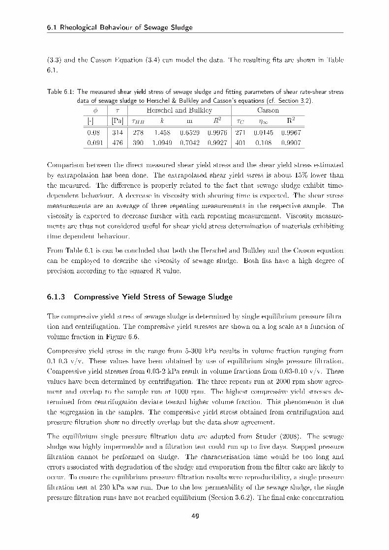
6.1 Rheological Behaviour of Sewage Sludge
(3.3) and the Casson Equation (3.4) can model the data. The resulting ts are shown in Table6.1.
Table 6.1: The measured shear yield stress of sewage sludge and tting parameters of shear rate-shear stressdata of sewage sludge to Herschel & Bulkley and Casson's equations (cf. Section 3.2).
φ τ Herschel and Bulkley Casson[-] [Pa] τHB k m R2 τC η∞ R2
0.08 314 278 1.458 0.6529 0.9976 271 0.0145 0.99670.091 476 390 1.0949 0.7042 0.9927 401 0.108 0.9907
Comparison between the direct measured shear yield stress and the shear yield stress estimatedby extrapolation has been done. The extrapolated shear yield stress is about 15% lower thanthe measured. The dierence is properly related to the fact that sewage sludge exhibit time-dependent behaviour. A decrease in viscosity with shearing time is expected. The shear stressmeasurements are an average of three repeating measurements in the respective sample. Theviscosity is expected to decrease further with each repeating measurement. Viscosity measure-ments are thus not considered useful for shear yield stress determination of materials exhibitingtime-dependent behaviour.
From Table 6.1 is can be concluded that both the Herschel and Bulkley and the Casson equationcan be employed to describe the viscosity of sewage sludge. Both ts have a high degree ofprecision according to the squared R value.
6.1.3 Compressive Yield Stress of Sewage Sludge
The compressive yield stress of sewage sludge is determined by single equilibrium pressure ltra-tion and centrifugation. The compressive yield stresses are shown on a log scale as a function ofvolume fraction in Figure 6.6.
Compressive yield stress in the range from 5-300 kPa results in volume fraction ranging from0.1-0.3 v/v. These values have been obtained by use of equilibrium single pressure ltration.Compressive yield stresses from 0.03-2 kPa result in volume fractions from 0.03-0.10 v/v. Thesevalues have been determined by centrifugation. The three repeats run at 2000 rpm show agree-ment and overlap to the sample run at 1000 rpm. The highest compressive yield stresses de-termined from centrifugation deviate toward higher volume fraction. This phenomenon is duethe segregation in the samples. The compressive yield stress obtained from centrifugation andpressure ltration show no directly overlap but the data show agreement.
The equilibrium single pressure ltration data are adapted from Studer (2008). The sewagesludge was highly impermeable and a ltration test could run up to ve days. Stepped pressureltration cannot be performed on sludge. The characterisation time would be too long anderrors associated with degradation of the sludge and evaporation from the lter cake are likely tooccur. To ensure the equilibrium pressure ltration results were reproducibility, a single pressureltration test at 230 kPa was run. Due to the low permeability of the sewage sludge, the singlepressure ltration runs have not reached equilibrium (Section 3.6.2). The nal cake concentration
49
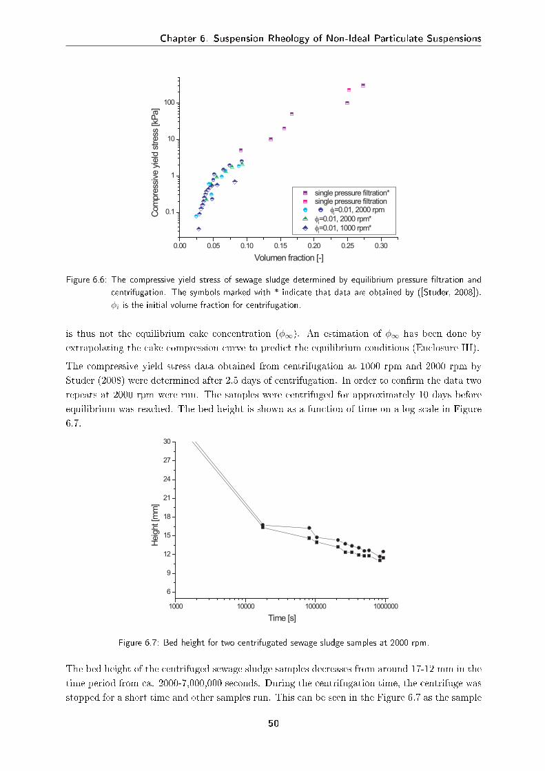
Chapter 6. Suspension Rheology of Non-Ideal Particulate Suspensions
0.00 0.05 0.10 0.15 0.20 0.25 0.30
0.1
1
10
100
single pressure filtration* single pressure filtration
φi=0.01, 2000 rpm
φi=0.01, 2000 rpm*
φi=0.01, 1000 rpm*
Com
pre
ssiv
e y
ield
stress
[kP
a]
Volumen fraction [-]
Figure 6.6: The compressive yield stress of sewage sludge determined by equilibrium pressure ltration andcentrifugation. The symbols marked with * indicate that data are obtained by ([Studer, 2008]).φi is the initial volume fraction for centrifugation.
is thus not the equilibrium cake concentration (φ∞). An estimation of φ∞ has been done byextrapolating the cake compression curve to predict the equilibrium conditions (Enclosure III).The compressive yield stress data obtained from centrifugation at 1000 rpm and 2000 rpm byStuder (2008) were determined after 2.5 days of centrifugation. In order to conrm the data tworepeats at 2000 rpm were run. The samples were centrifuged for approximately 10 days beforeequilibrium was reached. The bed height is shown as a function of time on a log scale in Figure6.7.
1000 10000 100000 1000000
6
9
12
15
18
21
24
27
30
Heig
ht [m
m]
Time [s]
Figure 6.7: Bed height for two centrifugated sewage sludge samples at 2000 rpm.
The bed height of the centrifuged sewage sludge samples decreases from around 17-12 mm in thetime period from ca. 2000-7,000,000 seconds. During the centrifugation time, the centrifuge wasstopped for a short time and other samples run. This can be seen in the Figure 6.7 as the sample
50
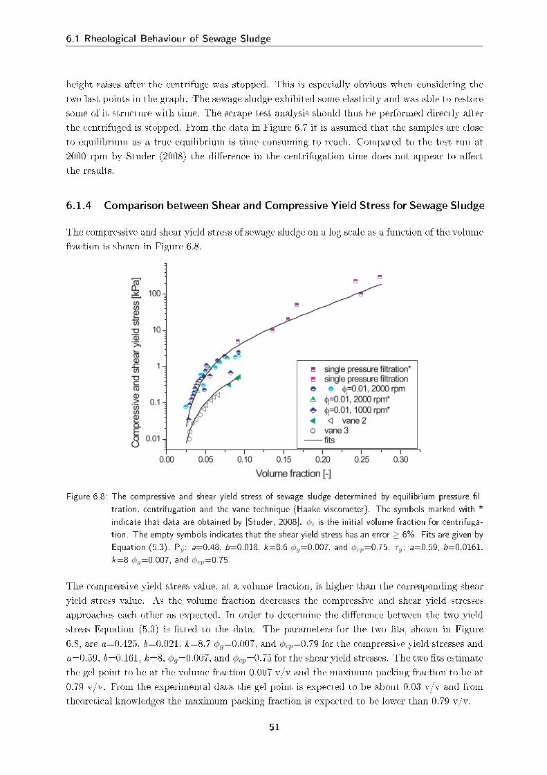
6.1 Rheological Behaviour of Sewage Sludge
height raises after the centrifuge was stopped. This is especially obvious when considering thetwo last points in the graph. The sewage sludge exhibited some elasticity and was able to restoresome of it structure with time. The scrape test analysis should thus be performed directly afterthe centrifuged is stopped. From the data in Figure 6.7 it is assumed that the samples are closeto equilibrium as a true equilibrium is time consuming to reach. Compared to the test run at2000 rpm by Studer (2008) the dierence in the centrifugation time does not appear to aectthe results.
6.1.4 Comparison between Shear and Compressive Yield Stress for Sewage Sludge
The compressive and shear yield stress of sewage sludge on a log scale as a function of the volumefraction is shown in Figure 6.8.
0.00 0.05 0.10 0.15 0.20 0.25 0.30
0.01
0.1
1
10
100
single pressure filtration* single pressure filtration
φi=0.01, 2000 rpm
φi=0.01, 2000 rpm*
φi=0.01, 1000 rpm*
vane 2 vane 3 fits
Com
pre
ssiv
e a
nd s
hear yi
eld
stress
[kP
a]
Volume fraction [-]
Figure 6.8: The compressive and shear yield stress of sewage sludge determined by equilibrium pressure l-tration, centrifugation and the vane technique (Haake viscometer). The symbols marked with *indicate that data are obtained by [Studer, 2008]. φi is the initial volume fraction for centrifuga-tion. The empty symbols indicates that the shear yield stress has an error ≥ 6%. Fits are given byEquation (5.3). Py: a=0.48, b=0.018, k=8.6 φg=0.007, and φcp=0.75. τy: a=0.59, b=0.0161,k=8 φg=0.007, and φcp=0.75.
The compressive yield stress value, at a volume fraction, is higher than the corresponding shearyield stress value. As the volume fraction decreases the compressive and shear yield stressesapproaches each other as expected. In order to determine the dierence between the two yieldstress Equation (5.3) is tted to the data. The parameters for the two ts, shown in Figure6.8, are a=0.425, b=0.021, k=8.7 φg=0.007, and φcp=0.79 for the compressive yield stresses anda=0.59, b=0.161, k=8, φg=0.007, and φcp=0.75 for the shear yield stresses. The two ts estimatethe gel point to be at the volume fraction 0.007 v/v and the maximum packing fraction to be at0.79 v/v. From the experimental data the gel point is expected to be about 0.03 v/v and fromtheoretical knowledges the maximum packing fraction is expected to be lower than 0.79 v/v.
51
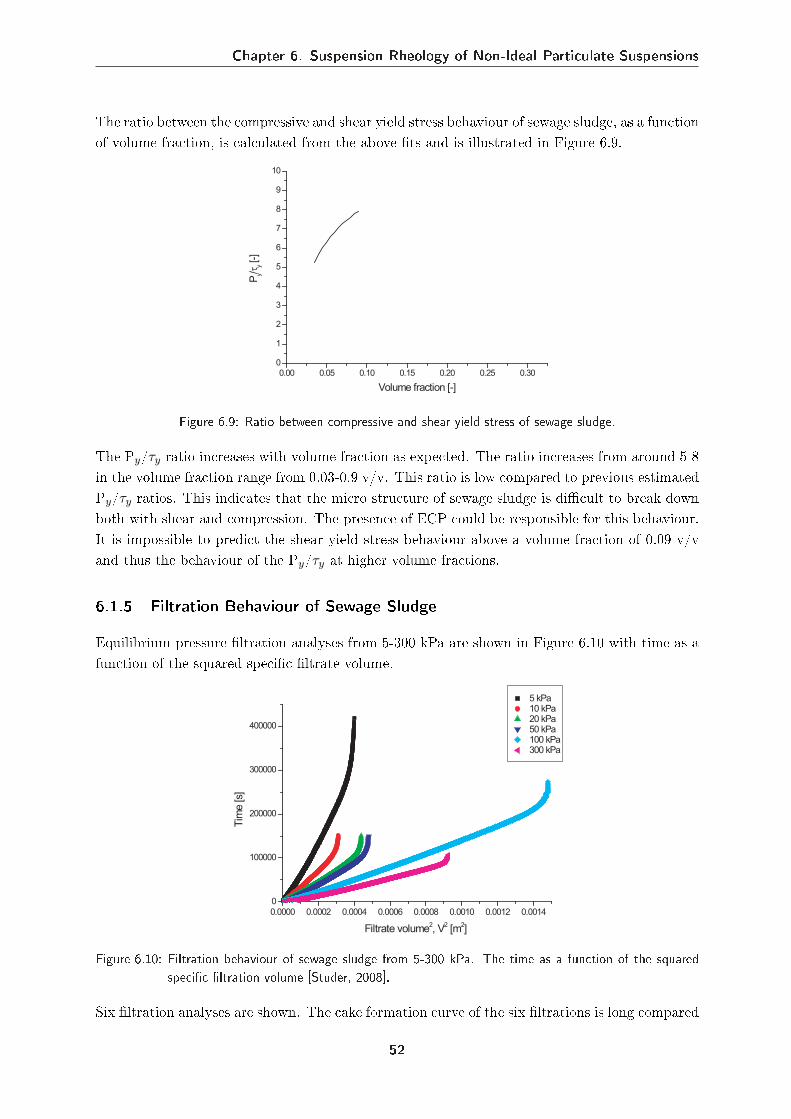
Chapter 6. Suspension Rheology of Non-Ideal Particulate Suspensions
The ratio between the compressive and shear yield stress behaviour of sewage sludge, as a functionof volume fraction, is calculated from the above ts and is illustrated in Figure 6.9.
0.00 0.05 0.10 0.15 0.20 0.25 0.30
0
1
2
3
4
5
6
7
8
9
10
Py/τ
y [-]
Volume fraction [-]
Figure 6.9: Ratio between compressive and shear yield stress of sewage sludge.
The Py/τy ratio increases with volume fraction as expected. The ratio increases from around 5-8in the volume fraction range from 0.03-0.9 v/v. This ratio is low compared to previous estimatedPy/τy ratios. This indicates that the micro structure of sewage sludge is dicult to break downboth with shear and compression. The presence of ECP could be responsible for this behaviour.It is impossible to predict the shear yield stress behaviour above a volume fraction of 0.09 v/vand thus the behaviour of the Py/τy at higher volume fractions.
6.1.5 Filtration Behaviour of Sewage Sludge
Equilibrium pressure ltration analyses from 5-300 kPa are shown in Figure 6.10 with time as afunction of the squared specic ltrate volume.
0.0000 0.0002 0.0004 0.0006 0.0008 0.0010 0.0012 0.0014
0
100000
200000
300000
400000
Tim
e [s]
Filtrate volume2, V
2 [m
2]
5 kPa 10 kPa 20 kPa 50 kPa 100 kPa 300 kPa
Figure 6.10: Filtration behaviour of sewage sludge from 5-300 kPa. The time as a function of the squaredspecic ltration volume [Studer, 2008].
Six ltration analyses are shown. The cake formation curve of the six ltrations is long compared
52
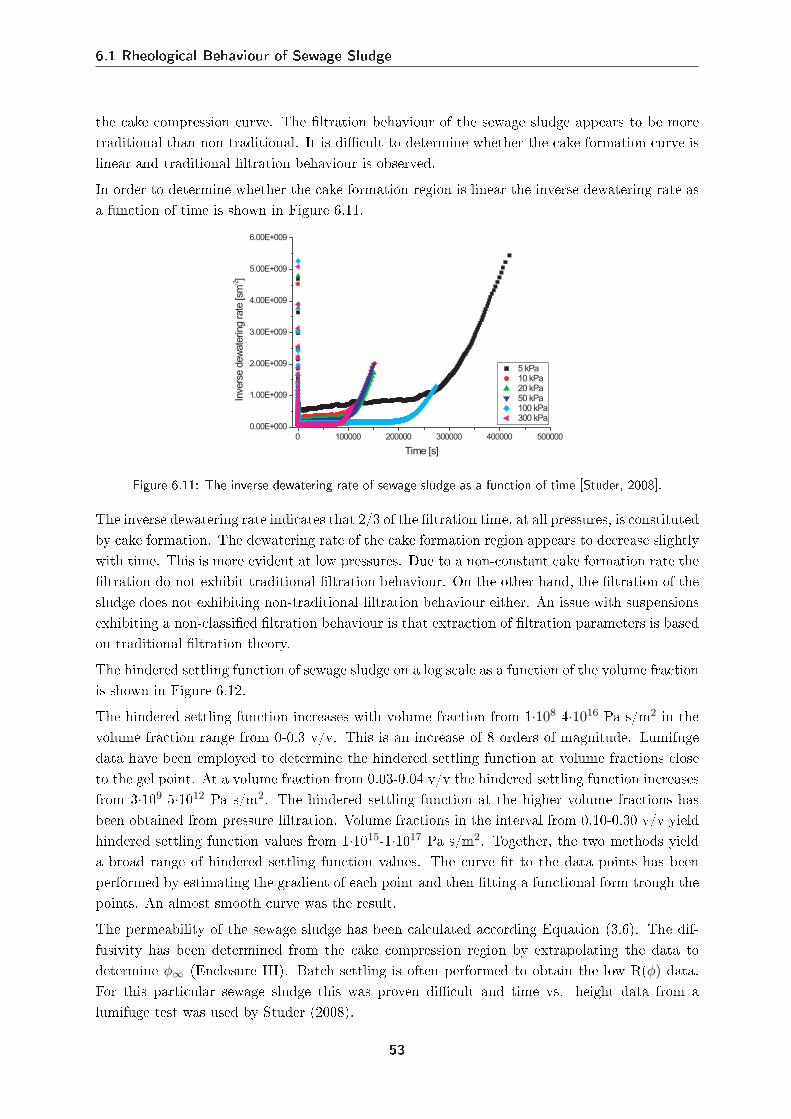
6.1 Rheological Behaviour of Sewage Sludge
the cake compression curve. The ltration behaviour of the sewage sludge appears to be moretraditional than non-traditional. It is dicult to determine whether the cake formation curve islinear and traditional ltration behaviour is observed.In order to determine whether the cake formation region is linear the inverse dewatering rate asa function of time is shown in Figure 6.11.
0 100000 200000 300000 400000 500000
0.00E+000
1.00E+009
2.00E+009
3.00E+009
4.00E+009
5.00E+009
6.00E+009In
vers
e d
ew
ate
ring rate
[sm
-2]
Time [s]
5 kPa 10 kPa 20 kPa 50 kPa 100 kPa 300 kPa
Figure 6.11: The inverse dewatering rate of sewage sludge as a function of time [Studer, 2008].
The inverse dewatering rate indicates that 2/3 of the ltration time, at all pressures, is constitutedby cake formation. The dewatering rate of the cake formation region appears to decrease slightlywith time. This is more evident at low pressures. Due to a non-constant cake formation rate theltration do not exhibit traditional ltration behaviour. On the other hand, the ltration of thesludge does not exhibiting non-traditional ltration behaviour either. An issue with suspensionsexhibiting a non-classied ltration behaviour is that extraction of ltration parameters is basedon traditional ltration theory.The hindered settling function of sewage sludge on a log scale as a function of the volume fractionis shown in Figure 6.12.The hindered settling function increases with volume fraction from 1·108-4·1016 Pa s/m2 in thevolume fraction range from 0-0.3 v/v. This is an increase of 8 orders of magnitude. Lumifugedata have been employed to determine the hindered settling function at volume fractions closeto the gel point. At a volume fraction from 0.03-0.04 v/v the hindered settling function increasesfrom 3·109-5·1012 Pa s/m2. The hindered settling function at the higher volume fractions hasbeen obtained from pressure ltration. Volume fractions in the interval from 0.10-0.30 v/v yieldhindered settling function values from 1·1015-1·1017 Pa s/m2. Together, the two methods yielda broad range of hindered settling function values. The curve t to the data points has beenperformed by estimating the gradient of each point and then tting a functional form trough thepoints. An almost smooth curve was the result.The permeability of the sewage sludge has been calculated according Equation (3.6). The dif-fusivity has been determined from the cake compression region by extrapolating the data todetermine φ∞ (Enclosure III). Batch settling is often performed to obtain the low R(φ) data.For this particular sewage sludge this was proven dicult and time vs. height data from alumifuge test was used by Studer (2008).
53
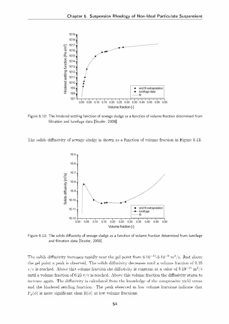
Chapter 6. Suspension Rheology of Non-Ideal Particulate Suspensions
0.00 0.05 0.10 0.15 0.20 0.25 0.30 0.35 0.40 0.45 0.50 0.55
1E7
1E8
1E9
1E10
1E11
1E12
1E13
1E14
1E15
1E16
1E17
1E18
1E19
end fit extrapolation lumifuge data fit
Hin
dere
d s
ettlin
g funct
ion [P
a s
/m2 ]
Volume fraction [-]
Figure 6.12: The hindered settling function of sewage sludge as a function of volume fraction determined fromltration and lumifuge data [Studer, 2008].
The solids diusivity of sewage sludge is shown as a function of volume fraction in Figure 6.13.
0.00 0.05 0.10 0.15 0.20 0.25 0.30 0.35 0.40 0.45 0.50
1E-12
1E-11
1E-10
1E-9
1E-8
1E-7
1E-6
1E-5
end fit extrapolation lumifuge fit
Solid
s diff
usi
vity
[m
2 /s]
Volume fraction [-]
Figure 6.13: The solids diusivity of sewage sludge as a function of volume fraction determined from lumifugeand ltration data [Studer, 2008].
The solids diusivity increases rapidly near the gel point from 6·10−11-5·10−9 m2/s. Just abovethe gel point a peak is observed. The solids diusivity decreases until a volume fraction of 0.15v/v is reached. Above this volume fraction the diusivity is constant at a value of 8·10−11 m2/suntil a volume fraction of 0.25 v/v is reached. Above this volume fraction the diusivity starts toincrease again. The diusivity is calculated from the knowledge of the compressive yield stressand the hindered settling function. The peak observed at low volume fractions indicate thatPy(φ) is more signicant than R(φ) at low volume fractions.
54
6.2 Summary of the Rheological Behaviour of Sewage Sludge
6.2 Summary of the Rheological Behaviour of Sewage Sludge
The characterised sewage sludge exhibited shear thinning behaviour and was thixotropic. Ex-trapolation of shear rate vs. shear rate data to a zero shear rate could not be employed todetermine the shear yield stress due to the time dependency of the material.
The sewage sludge was concentrated by centrifugation. Shear yield stress data above a volumefraction of 0.09 v/v could not be obtained due to the high impermeability of the sewage sludge.Uncertain shear yield stress values, at low volume fractions, were determined due to a limitedamount of sample. Compressive yield stresses could be obtained in the volume fraction rangefrom 0.03-0.30 v/v. The ratio between compression and shear was determined to increase from5.5-8 in the volume fraction range from 0.03-0.9 v/v.
The sewage sludge exhibited a non-classied ltration behaviour. The cake formation time con-stituted 2/3 of the ltration time and a weak decrease in dewatering rate during cake formationwas observed. The hindered settling function increased rapidly with volume fraction about 9orders of magnitude. The solids diusivity of the sewage sludge was low at a value about 1·10−10
m2/s. A maximum, at low volume fractions, was observed in the solids diusivity curve t.
55
Chapter 6. Suspension Rheology of Non-Ideal Particulate Suspensions
6.3 Rheological Behaviour of the Dual-Polymer-Flocculated Alu-mina Suspension
In this section a dual-polymer occulated alumina suspension is produced on basic of knowledgefrom previous investigations. The dual-polymer occulated alumina suspension behaviour inshear and compression is characterised. The ltration behaviour is presented in order to verify ifthe suspension exhibit non-traditional ltration behaviour as expected. Prediction of ltrationbehaviour of the suspension is performed on basis of the determined the hindered settling functionand compressive yield stresses.
6.3.1 Test of Polymer Dose for Dual-Polymer Flocculation of an Alumina Sus-pension
In the work done by Sutanto and Ho (2007), it was attempted to recreate a dual-occulated-system developed by Glover (2003). This proved dicult as no occulation occurred by additionof the prescribed polymer doses which are 10 ppm of PAA and 4 ppm of Zetag. The chosenpolymer doses which were 280 ppm of PAA and 140 ppm of Magnaoc LT20 did not result innon-traditional ltration behaviour. Dierent polymer doses were thus tried with the assumptionthat creation of larger ocs possibly would result in non-traditional ltration behaviour.The dierent PAA doses tested are shown in Table 6.2.
Table 6.2: Polymer doses tried for occulation of alumina suspensions. A concentration of 652 ppm PAA ischosen before the second polymer (Magnaoc LT20) is added.
PAA [ppm] Supernatant Magnaoc SupernatantLT20 [ppm]
300 non-clear 50 non-clear500 non-clear 200 non-clear697 non-clear 445 non-clear652 clear 392 clear699 clear 597 clear1177 clear 699 clear
1177 clear
Dilute alumina suspensions were prepared and the pH was adjusted to 5.5 before they wereleft overnight. The criteria for an optimum polymer dose was in this work dened as a reason-ably clear supernatant after occulation which together with the settling rate can help indicatewhether reproducible occulation can be obtained (Figure 6.14). As only weak occulationoccurred after addition of 280 ppm of PAA doses from 300 ppm and above were tried.The nal chosen polymer doses were 652 ppm of PAA and 392 ppm of Magnaoc LT20 and thepH was raised to 7.29 as the occulation appeared to be more reproducible at this pH. The chosendoses are remarkably higher than the one used by Glover (2003). The electrolyte concentrationin this work is increased from 10−4M KNO3 to 10−3M KNO3 compared to Glover (2003) and thepH is increased from 5-7.5. A pH closer to the isoelectric point and a higher salt concentration
56
6.3 Rheological Behaviour of the Dual-Polymer-Flocculated Alumina Suspension
Figure 6.14: Suspensions after settling of the ocs. Left picture shows a non-clear supernatant and the rightpicture shows a more clear supernatant.
leads theoretically to a lower surface potential which is expected to require a lower dosage ofpolymer to occulate the suspension but this was not observed here.
The settling rate for occulation is 8·10−4 ms−1 if only PAA is added and 1.8·10−3±1.7·10−4
ms−1 when both PAA and Magnaoc LT20 are added. The volume fraction after settling andremoval of the supernatant was about 0.03 v/v. The suspension was concentration by means ofcentrifugation to obtain dierent volume fractions. The aggregate size after addition of PAA was86±3.5 µm and after addition of the Magnaoc LT20 the aggregate size increases to 189±2.6µm. In Figure 6.15 the size distribution is illustrated.
10 100 1000
0
2
4
6
8
10
12
Diff
ere
ntia
l volu
me p
erc
ent [%
]
Particle diameter [µm]
addition of PAA addition of PAA and Magnafloc
Figure 6.15: Particle diameter of occulated alumina suspensions (pH=7.3, 10−3M KNO3) with PolyacrylicAcid (PAA) and then a polyacrylamide polymer (Magnaoc).
A more narrow size distribution of the aggregates is observed after occulation with only PAAcompared to the dual-polymer occulation.
57
Chapter 6. Suspension Rheology of Non-Ideal Particulate Suspensions
6.3.2 Shear Yield Stress of the Dual-Polymer Flocculated Alumina Suspension
The shear yield stress of the occulated alumina suspension on a log scale as a function of shearrate is shown in Figure 6.16.
0.10 0.15 0.20 0.25 0.30 0.35 0.40 0.45
0.01
0.1
1
10
vane 1* vane 1 vane 2 vane 3 vane 3
Shear yi
eld
stress
[kP
a]
Volume fraction [-]
Figure 6.16: Shear yield stress of occulated alumina suspension. * indicate data points obtained from mea-surements on the ARES rheometer and the remaining points are measured on the Haake Vis-cometer. The empty symbols indicates that the shear yield stress has an error ≥ 6%.
The shear yield stress increases with volume fraction. Shear yield stresses from 0.2-15 kPa weremeasured in the volume fraction range from 0.09-0.42 v/v. The occulated alumina suspensionwas easily concentrated by centrifugation to high volume fractions contrary to the sewage sludge.Due to the limited amount of sample, the measurements at the lowest volume fractions are as-sociated with error. At high shear yield stresses (>3 kPa) the ARES rheometer was used tomeasure the shear yield stress for the following reasons. A higher precision is obtained, the max-imum torque limit is not exceeded, and the cup is xed which will prevent the cup from turningduring the measurement. The last mentioned problem is an issue when high concentrations aremeasured on the Haake Viscometer.
58
6.3 Rheological Behaviour of the Dual-Polymer-Flocculated Alumina Suspension
6.3.3 Compressive Yield Stress of the Dual-Polymer Flocculated Alumina Sus-pension
The compressive yield stress is measured by both single and stepped pressure equilibrium ltra-tion, centrifugation, and batch settling. The compressive yield stress as a function of volumefraction is shown in Figure 6.17.
0.00 0.05 0.10 0.15 0.20 0.25 0.30 0.35 0.40 0.45
0.01
0.1
1
10
100
stepped pressure filtration single pressure filtration
φi=0.03, 1000 rpm
batch settling φav
Com
pre
ssiv
e y
ield
stress
[kP
a]
Volume fraction [-]
Figure 6.17: Compressive yield stresses as a function of volume fraction of a dual-polymer occulated aluminasuspension.
Compressive yield stress increases with volume fraction. The compressive yield stress has beendetermined in the stress interval from 0.04-300 kPa resulting i volume fractions from 0.05-0.45v/v. The lowest compressive yield stress data have been determined with batch settling. In thevolume fraction range from 0.05-0.10 no data was obtained. From 0.10-0.30 v/v, compressiveyield stress was determined by centrifugation. Agreement between the samples in duplicate isobserved. At volume fraction from 0.25-0.45 v/v compressive yield stress data from ltrationwere obtained. The compressive yield stress from single pressure ltration and centrifugationoverlaps.
The results obtained by single and stepped pressure equilibrium ltration deviate from eachother. It appears that the single pressure ltration results are in agreement and the steppedpressure ltrations results are erroneous. The results of the single pressure ltrations arise fromocculation of seven dierent sample and the stepped pressure ltration only from one sample.No dierence can be observed in the occulation rate, pH or conductivity between the samplesthat could indicate a change in the surface chemistry. A possible explanation could be that thesample used for the stepped pressure ltration run was left to settle in a tube (diameter=40 mm)for 5 days before the ltration. Aggregates in the bottom of the bed could to some extent bebroken up by the weight of the solid above. This would lead to formation of a denser cake. Allthe single pressure ltration tests were run immediately after the occulation process.
59
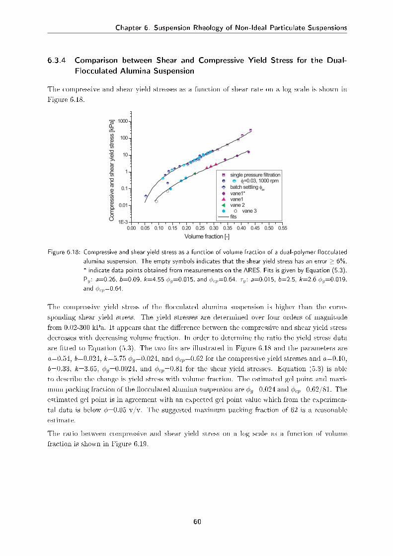
Chapter 6. Suspension Rheology of Non-Ideal Particulate Suspensions
6.3.4 Comparison between Shear and Compressive Yield Stress for the Dual-Flocculated Alumina Suspension
The compressive and shear yield stresses as a function of shear rate on a log scale is shown inFigure 6.18.
0.00 0.05 0.10 0.15 0.20 0.25 0.30 0.35 0.40 0.45 0.50 0.55
1E-3
0.01
0.1
1
10
100
1000
single pressure filtration φ
i=0.03, 1000 rpm
batch settling φav
vane1* vane1 vane 2 vane 3 fitsC
om
pre
ssiv
e a
nd s
hear yi
eld
stress
[kP
a]
Volume fraction [-]
Figure 6.18: Compressive and shear yield stress as a function of volume fraction of a dual-polymer occulatedalumina suspension. The empty symbols indicates that the shear yield stress has an error ≥ 6%.* indicate data points obtained from measurements on the ARES. Fits is given by Equation (5.3).Py: a=0.26, b=0.09, k=4.55 φg=0.015, and φcp=0.64. τy: a=0.015, b=2.5, k=2.6 φg=0.019,and φcp=0.64.
The compressive yield stress of the occulated alumina suspension is higher than the corre-sponding shear yield stress. The yield stresses are determined over four orders of magnitudefrom 0.02-300 kPa. It appears that the dierence between the compressive and shear yield stressdecreases with decreasing volume fraction. In order to determine the ratio the yield stress dataare tted to Equation (5.3). The two ts are illustrated in Figure 6.18 and the parameters area=0.54, b=0.024, k=5.75 φg=0.024, and φcp=0.62 for the compressive yield stresses and a=0.10,b=0.33, k=3.65, φg=0.0024, and φcp=0.81 for the shear yield stresses. Equation (5.3) is ableto describe the change is yield stress with volume fraction. The estimated gel point and maxi-mum packing fraction of the occulated alumina suspension are φg=0.024 and φcp=0.62/81. Theestimated gel point is in agreement with an expected gel point value which from the experimen-tal data is below φ=0.05 v/v. The suggested maximum packing fraction of 62 is a reasonableestimate.
The ratio between compressive and shear yield stress on a log scale as a function of volumefraction is shown in Figure 6.19.
60
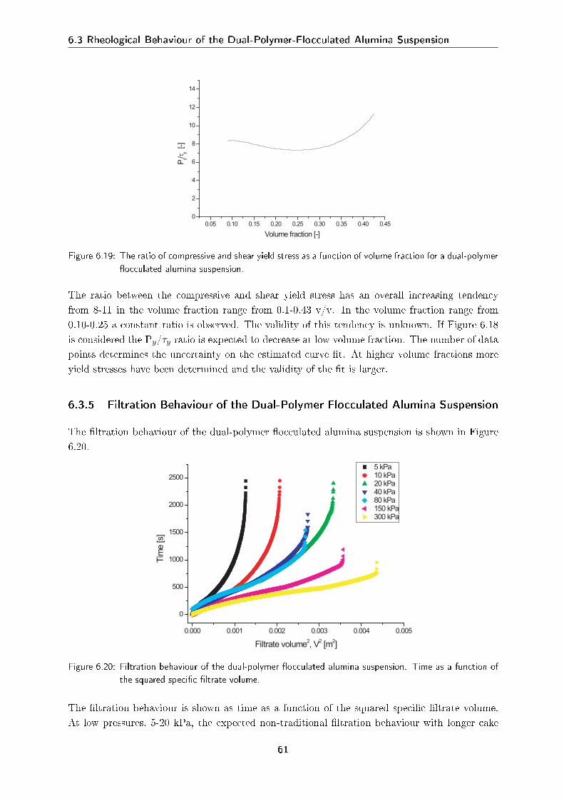
6.3 Rheological Behaviour of the Dual-Polymer-Flocculated Alumina Suspension
0.05 0.10 0.15 0.20 0.25 0.30 0.35 0.40 0.45
0
2
4
6
8
10
12
14
Py/τ
y [-]
Volume fraction [-]
Figure 6.19: The ratio of compressive and shear yield stress as a function of volume fraction for a dual-polymerocculated alumina suspension.
The ratio between the compressive and shear yield stress has an overall increasing tendencyfrom 8-11 in the volume fraction range from 0.1-0.43 v/v. In the volume fraction range from0.10-0.25 a constant ratio is observed. The validity of this tendency is unknown. If Figure 6.18is considered the Py/τy ratio is expected to decrease at low volume fraction. The number of datapoints determines the uncertainty on the estimated curve t. At higher volume fractions moreyield stresses have been determined and the validity of the t is larger.
6.3.5 Filtration Behaviour of the Dual-Polymer Flocculated Alumina Suspension
The ltration behaviour of the dual-polymer occulated alumina suspension is shown in Figure6.20.
0.000 0.001 0.002 0.003 0.004 0.005
0
500
1000
1500
2000
2500
Tim
e [s]
Filtrate volume2, V
2 [m
2]
5 kPa 10 kPa 20 kPa 40 kPa 80 kPa 150 kPa 300 kPa
Figure 6.20: Filtration behaviour of the dual-polymer occulated alumina suspension. Time as a function ofthe squared specic ltrate volume.
The ltration behaviour is shown as time as a function of the squared specic ltrate volume.At low pressures, 5-20 kPa, the expected non-traditional ltration behaviour with longer cake
61
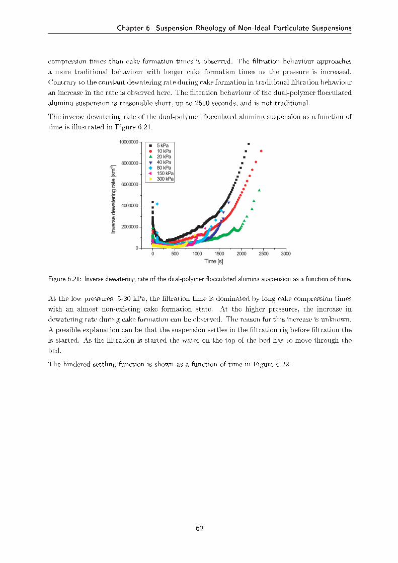
Chapter 6. Suspension Rheology of Non-Ideal Particulate Suspensions
compression times than cake formation times is observed. The ltration behaviour approachesa more traditional behaviour with longer cake formation times as the pressure is increased.Contrary to the constant dewatering rate during cake formation in traditional ltration behaviouran increase in the rate is observed here. The ltration behaviour of the dual-polymer occulatedalumina suspension is reasonable short, up to 2500 seconds, and is not traditional.
The inverse dewatering rate of the dual-polymer occulated alumina suspension as a function oftime is illustrated in Figure 6.21.
0 500 1000 1500 2000 2500 3000
0
2000000
4000000
6000000
8000000
10000000
Inve
rse d
ew
ate
ring rate
[sm
-2]
Time [s]
5 kPa 10 kPa 20 kPa 40 kPa 80 kPa 150 kPa 300 kPa
Figure 6.21: Inverse dewatering rate of the dual-polymer occulated alumina suspension as a function of time.
At the low pressures, 5-20 kPa, the ltration time is dominated by long cake compression timeswith an almost non-existing cake formation state. At the higher pressures, the increase indewatering rate during cake formation can be observed. The reason for this increase is unknown.A possible explanation can be that the suspension settles in the ltration rig before ltration theis started. As the ltration is started the water on the top of the bed has to move through thebed.
The hindered settling function is shown as a function of time in Figure 6.22.
62
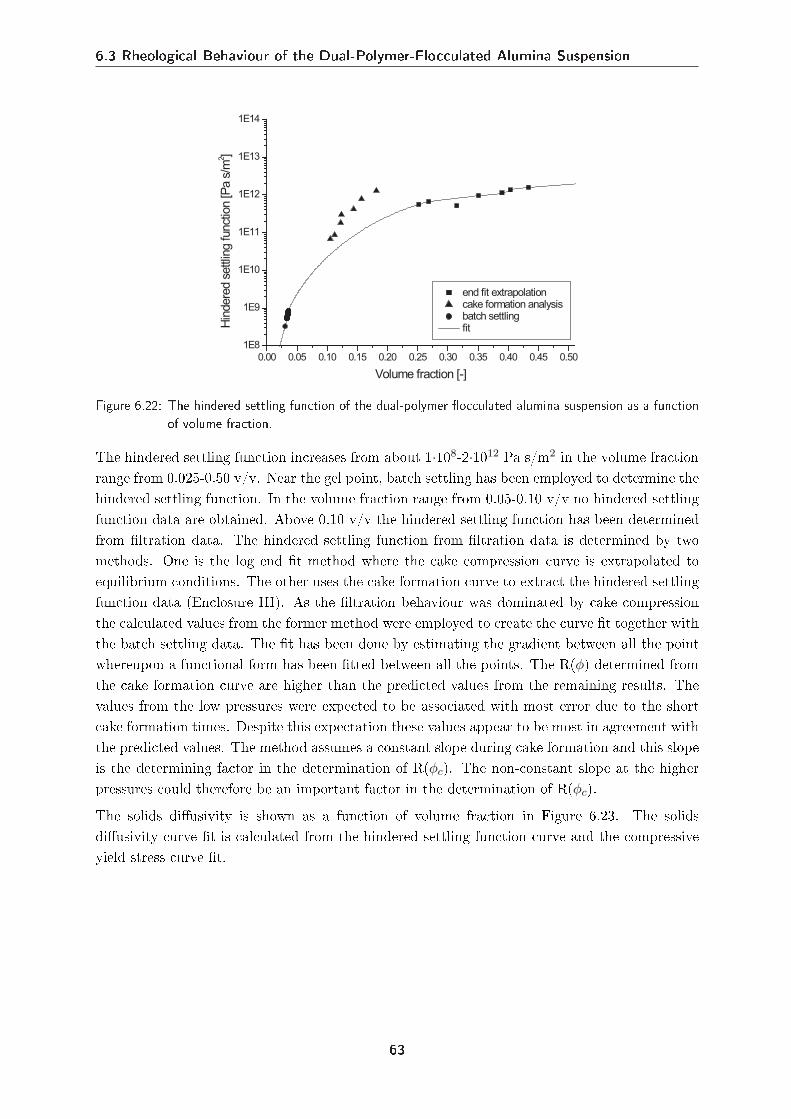
6.3 Rheological Behaviour of the Dual-Polymer-Flocculated Alumina Suspension
0.00 0.05 0.10 0.15 0.20 0.25 0.30 0.35 0.40 0.45 0.50
1E8
1E9
1E10
1E11
1E12
1E13
1E14
end fit extrapolation cake formation analysis batch settling fitH
indere
d s
ettlin
g funct
ion [P
a s
/m2 ]
Volume fraction [-]
Figure 6.22: The hindered settling function of the dual-polymer occulated alumina suspension as a functionof volume fraction.
The hindered settling function increases from about 1·108-2·1012 Pa s/m2 in the volume fractionrange from 0.025-0.50 v/v. Near the gel point, batch settling has been employed to determine thehindered settling function. In the volume fraction range from 0.05-0.10 v/v no hindered settlingfunction data are obtained. Above 0.10 v/v the hindered settling function has been determinedfrom ltration data. The hindered settling function from ltration data is determined by twomethods. One is the log end t method where the cake compression curve is extrapolated toequilibrium conditions. The other uses the cake formation curve to extract the hindered settlingfunction data (Enclosure III). As the ltration behaviour was dominated by cake compressionthe calculated values from the former method were employed to create the curve t together withthe batch settling data. The t has been done by estimating the gradient between all the pointwhereupon a functional form has been tted between all the points. The R(φ) determined fromthe cake formation curve are higher than the predicted values from the remaining results. Thevalues from the low pressures were expected to be associated with most error due to the shortcake formation times. Despite this expectation these values appear to be most in agreement withthe predicted values. The method assumes a constant slope during cake formation and this slopeis the determining factor in the determination of R(φc). The non-constant slope at the higherpressures could therefore be an important factor in the determination of R(φc).
The solids diusivity is shown as a function of volume fraction in Figure 6.23. The solidsdiusivity curve t is calculated from the hindered settling function curve and the compressiveyield stress curve t.
63
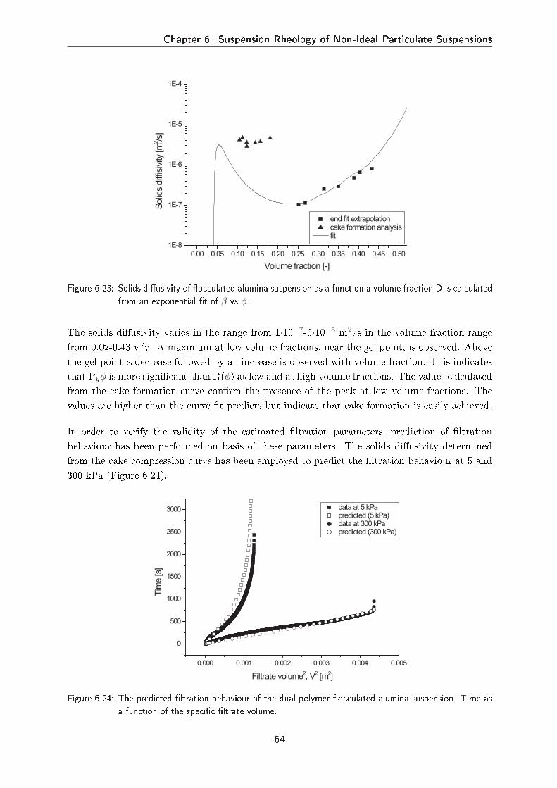
Chapter 6. Suspension Rheology of Non-Ideal Particulate Suspensions
0.00 0.05 0.10 0.15 0.20 0.25 0.30 0.35 0.40 0.45 0.50
1E-8
1E-7
1E-6
1E-5
1E-4
end fit extrapolation cake formation analysis fit
Solid
s diff
isiv
ity [m
2 /s]
Volume fraction [-]
Figure 6.23: Solids diusivity of occulated alumina suspension as a function a volume fraction D is calculatedfrom an exponential t of β vs φ.
The solids diusivity varies in the range from 1·10−7-6·10−5 m2/s in the volume fraction rangefrom 0.02-0.43 v/v. A maximum at low volume fractions, near the gel point, is observed. Abovethe gel point a decrease followed by an increase is observed with volume fraction. This indicatesthat Pyφ is more signicant than R(φ) at low and at high volume fractions. The values calculatedfrom the cake formation curve conrm the presence of the peak at low volume fractions. Thevalues are higher than the curve t predicts but indicate that cake formation is easily achieved.
In order to verify the validity of the estimated ltration parameters, prediction of ltrationbehaviour has been performed on basis of these parameters. The solids diusivity determinedfrom the cake compression curve has been employed to predict the ltration behaviour at 5 and300 kPa (Figure 6.24).
0.000 0.001 0.002 0.003 0.004 0.005
0
500
1000
1500
2000
2500
3000
Tim
e [s]
Filtrate volume2, V
2 [m
2]
data at 5 kPa predicted (5 kPa) data at 300 kPa predicted (300 kPa)
Figure 6.24: The predicted ltration behaviour of the dual-polymer occulated alumina suspension. Time asa function of the specic ltrate volume.
64
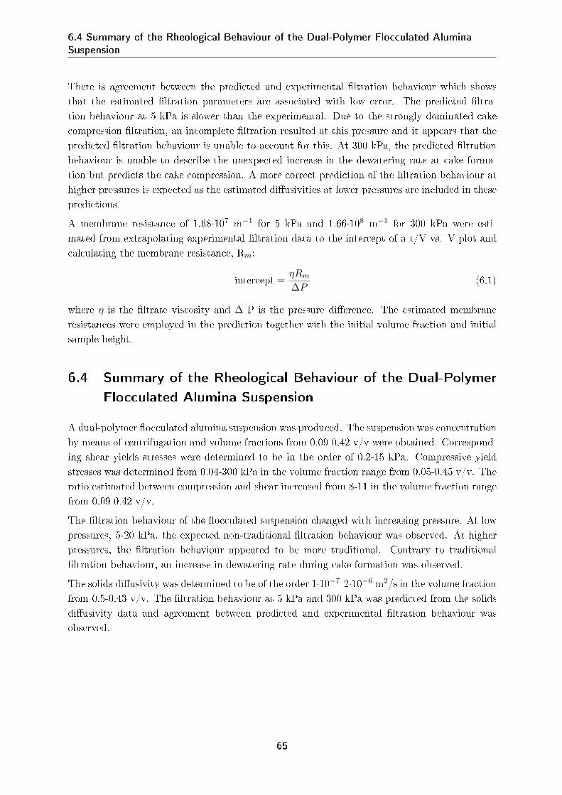
6.4 Summary of the Rheological Behaviour of the Dual-Polymer Flocculated AluminaSuspension
There is agreement between the predicted and experimental ltration behaviour which showsthat the estimated ltration parameters are associated with low error. The predicted ltra-tion behaviour at 5 kPa is slower than the experimental. Due to the strongly dominated cakecompression ltration, an incomplete ltration resulted at this pressure and it appears that thepredicted ltration behaviour is unable to account for this. At 300 kPa, the predicted ltrationbehaviour is unable to describe the unexpected increase in the dewatering rate at cake forma-tion but predicts the cake compression. A more correct prediction of the ltration behaviour athigher pressures is expected as the estimated diusivities at lower pressures are included in thesepredictions.
A membrane resistance of 1.68·107 m−1 for 5 kPa and 1.66·108 m−1 for 300 kPa were esti-mated from extrapolating experimental ltration data to the intercept of a t/V vs. V plot andcalculating the membrane resistance, Rm:
intercept =ηRm
∆P(6.1)
where η is the ltrate viscosity and ∆ P is the pressure dierence. The estimated membraneresistances were employed in the prediction together with the initial volume fraction and initialsample height.
6.4 Summary of the Rheological Behaviour of the Dual-PolymerFlocculated Alumina Suspension
A dual-polymer occulated alumina suspension was produced. The suspension was concentrationby means of centrifugation and volume fractions from 0.09-0.42 v/v were obtained. Correspond-ing shear yields stresses were determined to be in the order of 0.2-15 kPa. Compressive yieldstresses was determined from 0.04-300 kPa in the volume fraction range from 0.05-0.45 v/v. Theratio estimated between compression and shear increased from 8-11 in the volume fraction rangefrom 0.09-0.42 v/v.
The ltration behaviour of the occulated suspension changed with increasing pressure. At lowpressures, 5-20 kPa, the expected non-traditional ltration behaviour was observed. At higherpressures, the ltration behaviour appeared to be more traditional. Contrary to traditionalltration behaviour, an increase in dewatering rate during cake formation was observed.
The solids diusivity was determined to be of the order 1·10−7-2·10−6 m2/s in the volume fractionfrom 0.5-0.43 v/v. The ltration behaviour at 5 kPa and 300 kPa was predicted from the solidsdiusivity data and agreement between predicted and experimental ltration behaviour wasobserved.
65
Chapter 6. Suspension Rheology of Non-Ideal Particulate Suspensions
66
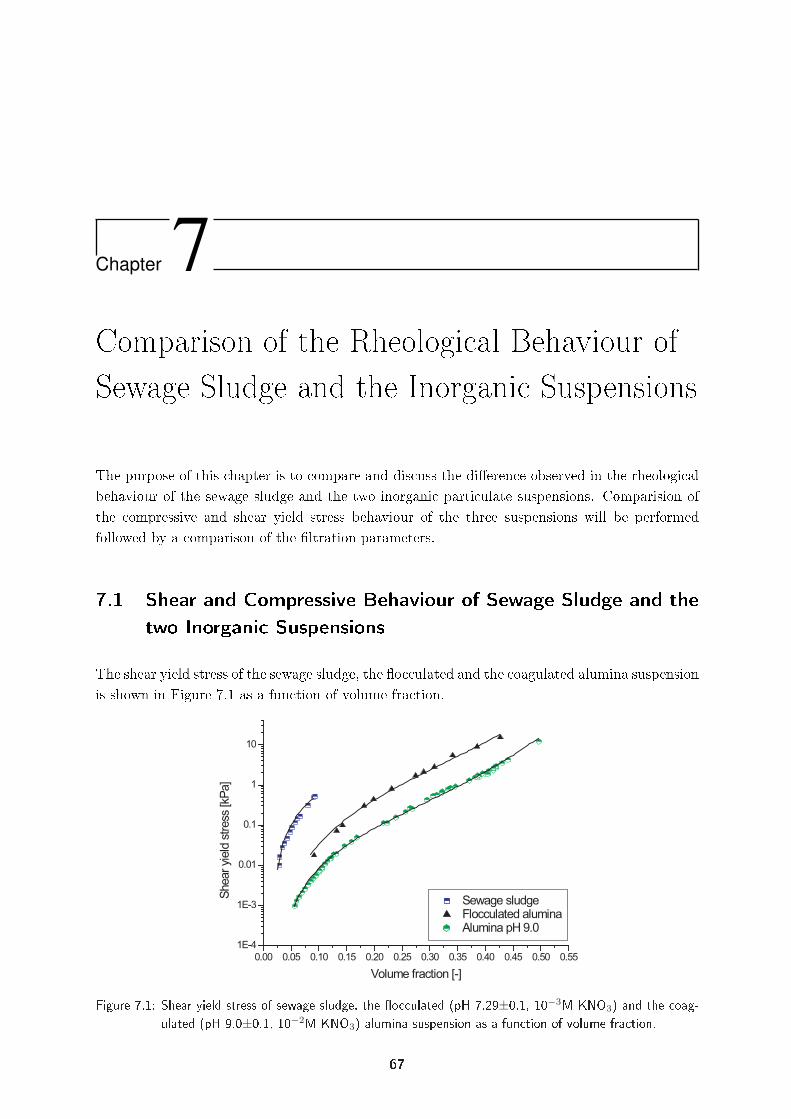
Chapter 7Comparison of the Rheological Behaviour ofSewage Sludge and the Inorganic Suspensions
The purpose of this chapter is to compare and discuss the dierence observed in the rheologicalbehaviour of the sewage sludge and the two inorganic particulate suspensions. Comparision ofthe compressive and shear yield stress behaviour of the three suspensions will be performedfollowed by a comparison of the ltration parameters.
7.1 Shear and Compressive Behaviour of Sewage Sludge and thetwo Inorganic Suspensions
The shear yield stress of the sewage sludge, the occulated and the coagulated alumina suspensionis shown in Figure 7.1 as a function of volume fraction.
0.00 0.05 0.10 0.15 0.20 0.25 0.30 0.35 0.40 0.45 0.50 0.55
1E-4
1E-3
0.01
0.1
1
10
Sewage sludge Flocculated alumina Alumina pH 9.0
Shear yi
eld
stress
[kP
a]
Volume fraction [-]
Figure 7.1: Shear yield stress of sewage sludge, the occulated (pH 7.29±0.1, 10−3M KNO3) and the coag-ulated (pH 9.0±0.1, 10−2M KNO3) alumina suspension as a function of volume fraction.
67
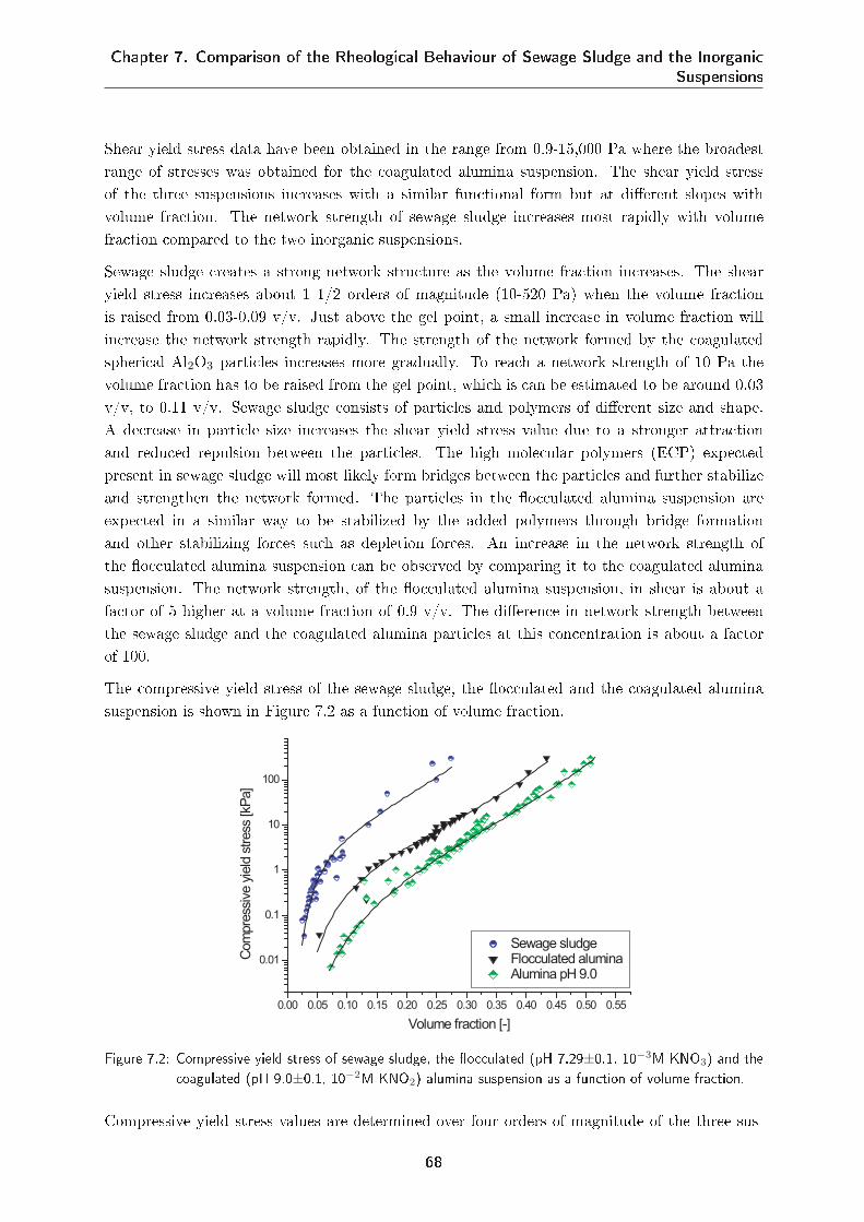
Chapter 7. Comparison of the Rheological Behaviour of Sewage Sludge and the InorganicSuspensions
Shear yield stress data have been obtained in the range from 0.9-15,000 Pa where the broadestrange of stresses was obtained for the coagulated alumina suspension. The shear yield stressof the three suspensions increases with a similar functional form but at dierent slopes withvolume fraction. The network strength of sewage sludge increases most rapidly with volumefraction compared to the two inorganic suspensions.
Sewage sludge creates a strong network structure as the volume fraction increases. The shearyield stress increases about 1 1/2 orders of magnitude (10-520 Pa) when the volume fractionis raised from 0.03-0.09 v/v. Just above the gel point, a small increase in volume fraction willincrease the network strength rapidly. The strength of the network formed by the coagulatedspherical Al2O3 particles increases more gradually. To reach a network strength of 10 Pa thevolume fraction has to be raised from the gel point, which is can be estimated to be around 0.03v/v, to 0.11 v/v. Sewage sludge consists of particles and polymers of dierent size and shape.A decrease in particle size increases the shear yield stress value due to a stronger attractionand reduced repulsion between the particles. The high molecular polymers (ECP) expectedpresent in sewage sludge will most likely form bridges between the particles and further stabilizeand strengthen the network formed. The particles in the occulated alumina suspension areexpected in a similar way to be stabilized by the added polymers through bridge formationand other stabilizing forces such as depletion forces. An increase in the network strength ofthe occulated alumina suspension can be observed by comparing it to the coagulated aluminasuspension. The network strength, of the occulated alumina suspension, in shear is about afactor of 5 higher at a volume fraction of 0.9 v/v. The dierence in network strength betweenthe sewage sludge and the coagulated alumina particles at this concentration is about a factorof 100.
The compressive yield stress of the sewage sludge, the occulated and the coagulated aluminasuspension is shown in Figure 7.2 as a function of volume fraction.
0.00 0.05 0.10 0.15 0.20 0.25 0.30 0.35 0.40 0.45 0.50 0.55
0.01
0.1
1
10
100
Sewage sludge Flocculated alumina Alumina pH 9.0
Com
pre
ssiv
e y
ield
stress
[kP
a]
Volume fraction [-]
Figure 7.2: Compressive yield stress of sewage sludge, the occulated (pH 7.29±0.1, 10−3M KNO3) and thecoagulated (pH 9.0±0.1, 10−2M KNO2) alumina suspension as a function of volume fraction.
Compressive yield stress values are determined over four orders of magnitude of the three sus-
68
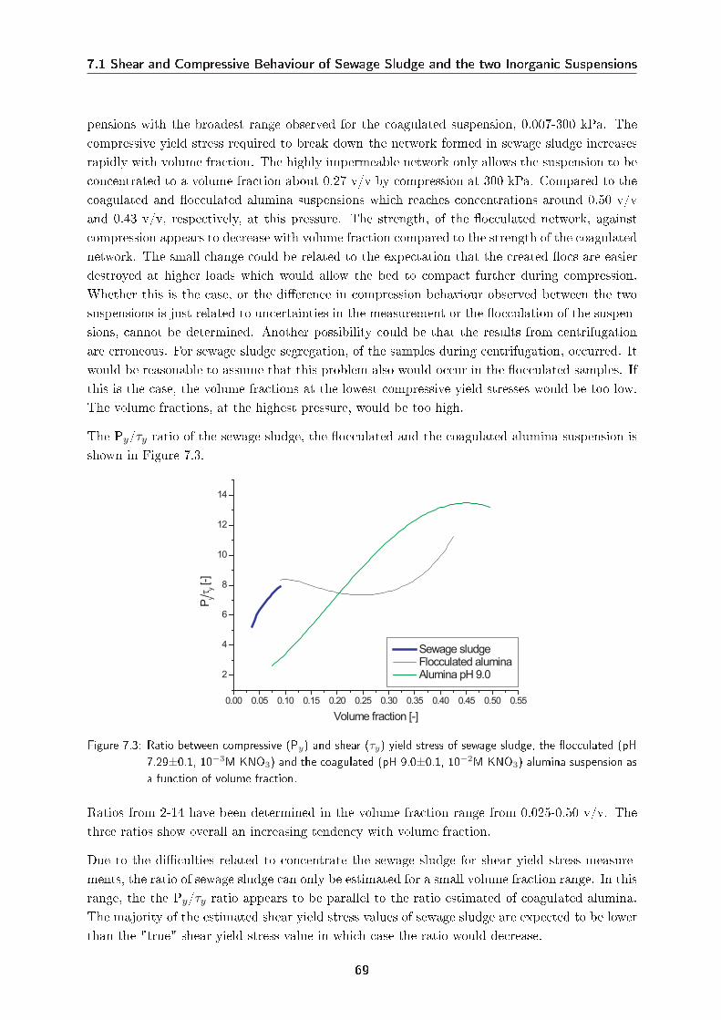
7.1 Shear and Compressive Behaviour of Sewage Sludge and the two Inorganic Suspensions
pensions with the broadest range observed for the coagulated suspension, 0.007-300 kPa. Thecompressive yield stress required to break down the network formed in sewage sludge increasesrapidly with volume fraction. The highly impermeable network only allows the suspension to beconcentrated to a volume fraction about 0.27 v/v by compression at 300 kPa. Compared to thecoagulated and occulated alumina suspensions which reaches concentrations around 0.50 v/vand 0.43 v/v, respectively, at this pressure. The strength, of the occulated network, againstcompression appears to decrease with volume fraction compared to the strength of the coagulatednetwork. The small change could be related to the expectation that the created ocs are easierdestroyed at higher loads which would allow the bed to compact further during compression.Whether this is the case, or the dierence in compression behaviour observed between the twosuspensions is just related to uncertainties in the measurement or the occulation of the suspen-sions, cannot be determined. Another possibility could be that the results from centrifugationare erroneous. For sewage sludge segregation, of the samples during centrifugation, occurred. Itwould be reasonable to assume that this problem also would occur in the occulated samples. Ifthis is the case, the volume fractions at the lowest compressive yield stresses would be too low.The volume fractions, at the highest pressure, would be too high.
The Py/τy ratio of the sewage sludge, the occulated and the coagulated alumina suspension isshown in Figure 7.3.
0.00 0.05 0.10 0.15 0.20 0.25 0.30 0.35 0.40 0.45 0.50 0.55
2
4
6
8
10
12
14
Sewage sludge Flocculated alumina Alumina pH 9.0
Py/τ
y [-]
Volume fraction [-]
Figure 7.3: Ratio between compressive (Py) and shear (τy) yield stress of sewage sludge, the occulated (pH7.29±0.1, 10−3M KNO3) and the coagulated (pH 9.0±0.1, 10−2M KNO3) alumina suspension asa function of volume fraction.
Ratios from 2-14 have been determined in the volume fraction range from 0.025-0.50 v/v. Thethree ratios show overall an increasing tendency with volume fraction.
Due to the diculties related to concentrate the sewage sludge for shear yield stress measure-ments, the ratio of sewage sludge can only be estimated for a small volume fraction range. In thisrange, the the Py/τy ratio appears to be parallel to the ratio estimated of coagulated alumina.The majority of the estimated shear yield stress values of sewage sludge are expected to be lowerthan the "true" shear yield stress value in which case the ratio would decrease.
69
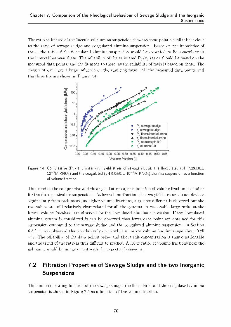
Chapter 7. Comparison of the Rheological Behaviour of Sewage Sludge and the InorganicSuspensions
The ratio estimated of the occulated alumina suspension shows to some point a similar behaviouras the ratio of sewage sludge and coagulated alumina suspension. Based on the knowledge ofthese, the ratio of the occulated alumina suspension would be expected to lie somewhere inthe interval between these. The reliability of the estimated Py/τy ratios should be based on themeasured data points, and the t made to those, as the reliability of ratio is based on these. Thechosen t can have a large inuence on the resulting ratio. All the measured data points andthe three ts are shown in Figure 7.4.
0.00 0.05 0.10 0.15 0.20 0.25 0.30 0.35 0.40 0.45 0.50 0.55
1E-3
0.01
0.1
1
10
100
Py, sewage sludge
τy, sewage sludge
Py, flocculated alumina
τy, flocculated alumina
Py, alumina pH 9.0
τy, alumina 9.0
Com
pre
ssiv
e a
nd s
hear yi
eld
stress
[kP
a]
Volume fraction [-]
Figure 7.4: Compressive (Py) and shear (τy) yield stress of sewage sludge, the occulated (pH 7.29±0.1,10−3M KNO3) and the coagulated (pH 9.0±0.1, 10−2M KNO3) alumina suspension as a functionof volume fraction.
The trend of the compressive and shear yield stresses, as a function of volume fraction, is similarfor the three particulate suspensions. At low volume fraction, the two yield stresses do not deviatesignicantly from each other, at higher volume fractions, a greater dierent is observed but thetwo values are still relatively close related for all the systems. A reasonable large ratio, at thelowest volume fractions, are observed for the occulated alumina suspension. If the occulatedalumina system is considered it can be observed that fewer data point are obtained for thissuspension compared to the sewage sludge and the coagulated alumina suspension. In Section6.3.3, it was observed that overlap only occurred at a narrow volume fraction range about 0.25v/v. The reliability of the data points below and above this concentration is thus questionableand the trend of the ratio is thus dicult to predict. A lower ratio, at volume fractions near thegel point, would be in agreement with the expected behaviour.
7.2 Filtration Properties of Sewage Sludge and the two InorganicSuspensions
The hindered settling function of the sewage sludge, the occulated and the coagulated aluminasuspension is shown in Figure 7.5 as a function of the volume fraction.
70
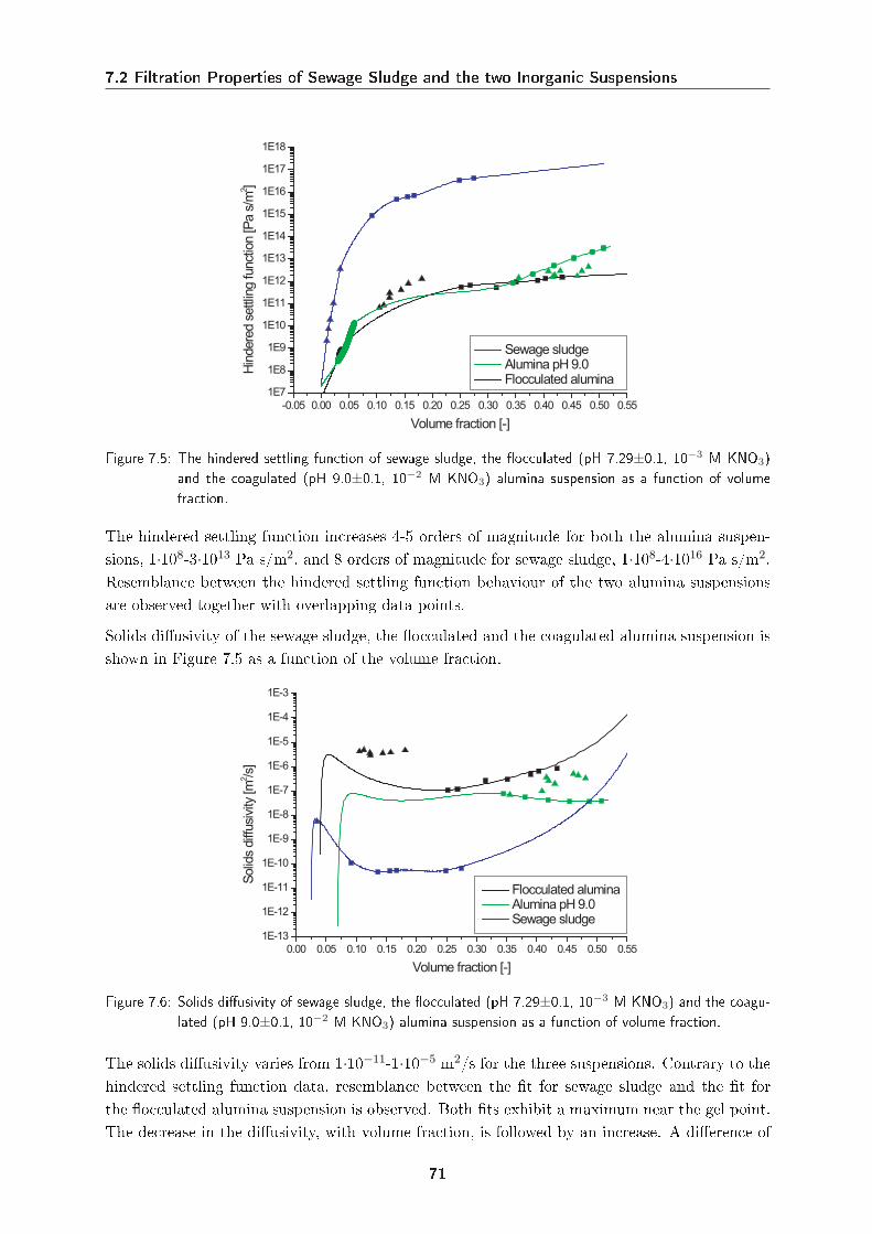
7.2 Filtration Properties of Sewage Sludge and the two Inorganic Suspensions
-0.05 0.00 0.05 0.10 0.15 0.20 0.25 0.30 0.35 0.40 0.45 0.50 0.55
1E7
1E8
1E9
1E10
1E11
1E12
1E13
1E14
1E15
1E16
1E17
1E18
Sewage sludge Alumina pH 9.0 Flocculated alumina
Hin
dere
d s
ettlin
g funct
ion [P
a s
/m2 ]
Volume fraction [-]
Figure 7.5: The hindered settling function of sewage sludge, the occulated (pH 7.29±0.1, 10−3 M KNO3)and the coagulated (pH 9.0±0.1, 10−2 M KNO3) alumina suspension as a function of volumefraction.
The hindered settling function increases 4-5 orders of magnitude for both the alumina suspen-sions, 1·108-3·1013 Pa s/m2, and 8 orders of magnitude for sewage sludge, 1·108-4·1016 Pa s/m2.Resemblance between the hindered settling function behaviour of the two alumina suspensionsare observed together with overlapping data points.
Solids diusivity of the sewage sludge, the occulated and the coagulated alumina suspension isshown in Figure 7.5 as a function of the volume fraction.
0.00 0.05 0.10 0.15 0.20 0.25 0.30 0.35 0.40 0.45 0.50 0.55
1E-13
1E-12
1E-11
1E-10
1E-9
1E-8
1E-7
1E-6
1E-5
1E-4
1E-3
Flocculated alumina Alumina pH 9.0 Sewage sludge
Solid
s diff
usi
vity
[m
2 /s]
Volume fraction [-]
Figure 7.6: Solids diusivity of sewage sludge, the occulated (pH 7.29±0.1, 10−3 M KNO3) and the coagu-lated (pH 9.0±0.1, 10−2 M KNO3) alumina suspension as a function of volume fraction.
The solids diusivity varies from 1·10−11-1·10−5 m2/s for the three suspensions. Contrary to thehindered settling function data, resemblance between the t for sewage sludge and the t forthe occulated alumina suspension is observed. Both ts exhibit a maximum near the gel point.The decrease in the diusivity, with volume fraction, is followed by an increase. A dierence of
71
Chapter 7. Comparison of the Rheological Behaviour of Sewage Sludge and the InorganicSuspensions
about 3 orders of magnitude is observed in the solids diusivity. From the knowledge about theltration behaviour of the two suspensions, the occulated alumina suspension cannot directlyact as a substitute to sewage sludge. On the other hand, the occulated alumina suspension couldbe an ideal suspension for understanding non-traditional ltration behaviour at low pressuresand then the transition to more traditional ltration behaviour at higher pressures.
72
Chapter 8Conclusion
The compressive and shear yield stress of sewage sludge, a coagulated alumina suspension, anda dual-polymer occulated alumina suspension increased as a function of volume fraction. Thethree suspensions were more easily deformed by shear than by compression. The Py/τy ratioof three suspensions increased with volume fraction in the investigated volume fraction ranges.The ratios appeared to have a similar shape. The ratio of the sewage sludge increased from 5-8in the volume fraction range from 0.035-0.09 v/v, the coagulated alumina suspension from 2-14in the volume fraction range from 0.075-0.50 v/v, and the occulated alumina suspension from8-11 in the volume fraction range from 0.09-0.43 v/v. The ratio determined for the coagulatedalumina suspension is in agreement with previous investigations done by Zhou (2000).
The compressive and shear yield stress of sewage sludge increased more rapidly with volumefraction than was the case for the alumina suspensions. Small particles and the ECP in sewagesludge are believed to be responsible for sewage sludge's stronger three dimensional networkstructure. The occulated alumina suspension exhibited a stronger network structure as a func-tion of volume fraction than the coagulated alumina suspension did, which can be ascribed topolymer eects as bridging and depletion forces.
The coagulated alumina suspension exhibited traditional ltration behaviour with a linear dom-inating cake formation state and short cake compression times. The hindered settling functionof the suspensions increased over 5 orders of magnitude, from 1·108-3·1013 Pa s/m2, with volumefraction. The solids diusivity of the suspension was almost independent of volume fraction at1·10−7 m2/s. Sewage sludge did not exhibit non-traditional ltration behaviour as expected. Amore traditional ltration behaviour, with long formation times with a weak decreasing dewater-ing rate, was observed. The hindered settling function of sewage sludge increased over 8 ordersof magnitude, 1·108-4·1016 Pa s/m2, with volume fraction. The solids diusivity of sewage sludgevaried from 6·10−11-5·10−9 m2/s and showed a maximum near the gel point and the decrease withvolume fraction was followed by an increase. Non-tradional ltration behaviour was observedat low pressures, 5-40 kPa, for the occulated alumina suspension. A short almost non-existingcake formation was followed by long cake compression times. At the higher pressures, a weak in-creasing dewatering rate in cake formation was followed by shorter cake compression times. Thehindered settling function of the suspensions was determined to increase from 1·108-1·1012 Pa
73
Chapter 8. Conclusion
s/m2. The occulated alumina suspension exhibited a similar solids diusivity behaviour withvolume fraction as the sewage sludge thus three orders of magnitude larger, 1·10−7-2·10−6 m2/s.Determination of ltration parameters, from linarisation of the cake compression region, resultedin reasonable prediction of the ltration behaviour of the occulated alumina suspension.
74
Bibliography
[Ackerson, 1990] B. J. Ackerson. Shear Induced Order and Shear Processing of Model HardSphere Suspensions. J. Rheol, 34(4):553590, May 1990.
[Aziz, 2004] A.A.A. Aziz. Characterisation of Shear Upon Dewaterability of Colloidal Suspen-sions. PhD thesis, University of Melbourne, Parkville, Victoria, Australia, 2004.
[Barnes and Walters, 1985] H. A. Barnes and K. Walters. The Yield Stress Myth? RheologicaActa, 24:323326, 1985.
[Barnes et al., 1989] H.A. Barnes , J.F. Hutton, and K. Walters. An Introduction to Rheology.Elsevier Science Publishers B.V, Amsterdam, The Nederlands, 1989.
[Barnes, 1997] H.A. Barnes. Thixtropy- a review. J. Non-Newtonian Fluid Mechanics, 70:133,Jan 1997.
[Barnes, 2000] H.A. Barnes. A Handbook of Elementary Rheology. Institute of Non-NewtonianFluid Mechanics, University of Wales, 2000.
[Bingham and Green, 1920] E.C. Bingham and H. Green. Paint a Plastic Material and not aViscous Liquid; the Measurements of its Mobility and Yiled Value. Proc. Am. Soc. Test. Matl.,20:640675, 1920.
[Buscall and White, 1987] R. Buscall and L.R. White. The Consolidation of Concentrated Sus-pensions. Journal of Chemical Society Faraday Transactions, 83:873891, 1987.
[Buscall et al., 1987] R. Buscall , I.J. McGowan , P.D.A Mills , R.F. Stewart , D. Sutton , L.R.white, and G.E. Yates. The Rheology of Strongly-Flocculated Suspensions. Journal of Non-Newtonian Fluid Mechanics, 24:183202, 1987.
[Channel and Zukoski, 1997] G.M. Channel and C.F. Zukoski. Shear and Compressive Rheologyof Aggregated Alumina Suspensions? AIChE Journal, 43(7):17001708, July 1997.
[Chhabra, 2007] R. P Chhabra. Bubbles, Drops, and Particles in Non-Newtonian Fluids. CRCPress, 2007.
75
BIBLIOGRAPHY
[de Kretser et al., 2005] R.G. de Kretser , S.P.Usher, and P.J. Scales. Comprehensive DewateringBehaviour Analysis for Fine and Flocculated Materials. Proceedings of American Filtrationand Seperation Society, April 10-13 2005.
[Dignac et al., 2007] M.F. Dignac , V. Urbain , D. Rybacki , A. Bruchet , D. Snidaro, andP. Scribe. Chemical Description of Extracellular Polymers: Implication on Wastewater Sludge.Water Research, 41:206216, 2007.
[Glover et al., 2004] S.M. Glover , Y. Yan , G.J. Jameson, and S. Biggs. Dewatering Propertiesof Dual-Polymer-Flocculated Systems. Int. J. Miner. Process., 73:145160, 2004.
[Glover, 2003] S.M. Glover. Novel Routes for Polymer-Assisted Solid-Liquid Separation. Ph.Dthesis, The University of Newcastle, 2003.
[Goodwin and Hughes, 2000] J.W. Goodwin and R.W Hughes. Rheology for Chemists An Intro-duction. The Royal Society of Chemistry, 2000.
[Green, 1997] M.D. Green. Characterisation of Suspensions in Settling and Compression. PhDthesis, University of Melbourne, Parkville, Victoria, Australia, 1997.
[Hartnett and Hu, 1989] J.P. Hartnett and R.Y.Z. Hu. Technical Note: The Yield Stress- AnEngeneering Relity. Journal of Rheology, 33(4):671679, 1989.
[Herschel and Bulkley, 1926] V. W. H. Herschel and R. Bulkley. Konsistenzmessungen vonGummi-Benzollosungen. Kolloid Zeit, 39:291300, 1926.
[Hiemenz and Rajagopalan, 1997] P. C. Hiemenz and R. Rajagopalan. Principles of Colloid andSurface Chemistry. Marcel Dekker, Inc., thrid edition, 1997.
[Hough and White, 1980] D.B. Hough and L.R. White. The Calculation of Hamaker Constantsfrom Lifshitz Theory with Applications to Wetting Phenomena. Adv. Colloid Interface Sci.,14:341, 1980.
[Hulston, 2005] J. Hulston. Eect of Flocculation Conditions on the Dewaterability of Hematiteand Red Mud Suspensions. PhD thesis, University of Melbourne, Parkville, Victoria, Australia,2005.
[Israelachvili, 1992] J. Israelachvili. Intermolecular and Surface forces. Academic Press, ElsevierScience, California USA, 1992.
[James et al., 1987] A.E. James , D.J.A. Williams, and P.R. Williams. Direct Measurement ofStatic Yield Properties of Cohesive Suspensions. Rheologica Acta, 26:437446, 1987.
[Johnson et al., 2000] S. B. Johnson , G. V. Franks , P.J. Scales , D.V. Boger, and T.W. Healy.Surface Chemistry- Rheology Relationships in Concentrated Mineral Suspensions. Interna-tional Journal of Mineral Processing, 58:267304, 2000.
[Kapur et al., 1997] P.C. Kapur , P.J. Scales , D.V. Boger, and T.W. Healy. Yield Stress ofSuspensions Loaded with Size Distributed Particles. AIChE Journal, 43(5):11711179, May1997.
76
BIBLIOGRAPHY
[Landman and White, 1994] K.A. Landman and L.R. White. Solid/Liquid Separation of Floc-culated Suspensions. Advances in Colloid and Interface Science, 51:175246, 1994.
[Landman and White, 1997] K.A. Landman and L.R. White. Predicting Filtration Time andMaximizing Throughput in a Pressure Filter. AIChE Journal, 43(12):31473160, Dec 1997.
[Landman et al., 1995] K.A. Landman , L.R. White, and M. Eberl. Pressure Filtration of Floc-culated Suspensions. AIChE Journal, 41(7):16871700, July 1995.
[Landman et al., 1999] K.A. Landman , J.M. Stankovich, and L.R. White. Measurement of theFiltration Diusivity D(φ) of a Flocculated Suspension. AIChE Journal, 45(9):18751882, Sep1999.
[Leong et al., 1995] Y.K Leong , P.J Scales , T.W. Healy, and D.V. Boger. Eect of Particle Sizeon Colloidal Zirconia Rheology at the Isoelectric Point. Journal of American Ceramic Society,78:22092212, 1995.
[Lester et al., 2005] D.R. Lester , S.P. Usher, and P.J. Scales. Estimation of the Hindered SettlingFunction R(φ) from Batch-Settling Tests. American Institute of Chemical Engineers, 51(4),April 2005.
[Liddell and Boger, 1995] P.V. Liddell and D.V. Boger. Yield Stress Measurement with the Vane.Journal of non-Newtonian Fluid Mechanics, 63:235261, 1995.
[Mascosko, 1994] C.W. Mascosko. Rheology: Principles, Measurements, and Application. VCHPublishers, New York, 1994.
[Meeten, 1994] G.H. Meeten. Shear and Compressive Yield in the Filtration of a BentoniteSuspension. Colloid and Surfaces, 82:7783, 1994.
[Miller et al., 1996] K.T. Miller , R.M. Melant, and C.F. Zukoski. Comparison of the Com-pressive Yield Response of Aggregated Suspensions: Pressure Filtration, Centrifugation, andOsmotic Consolidation. Journal of Ceramic Society, 79(10):254556, 1996.
[Nguyen and Boger, 1983] Q.D. Nguyen and D.V. Boger. Yield Stress Measurement for Concen-trated Suspensions. Journal of Rheology, 27(4):321349, 1983.
[Nguyen and Boger, 1985] Q.D. Nguyen and D.V. Boger. Direct Yield Stress Measurement withthe Vane Method. Journal of Rheology, 29(3):335347, 1985.
[Nguyen and Boger, 1992] Q.D. Nguyen and D.V. Boger. Measuring the Flow Properties of YielsStress Fluids. Annual Reviews Fluid Mechanics, 24:4788, 1992.
[Ohshima, 2006] H. Ohshima. Theory of Colloid and Interfacial Electric Phenomena. AcademicPress, Elsevier Science, Amsterdam, The Netherlands, 2006.
[Rheology Solutions Pty Ltd, 2008] Rheology Solutions Pty Ltd.http://www.rheologysolutions.com/viscotester550_techs.html, march 2008.
[Ruth et al., 1933] B.F. Ruth , G.H. Montillon, and R.E. Montonna. Studies in Filtration: ICritical Analysis of Filtration Theory. Industrial and Engineering Chemistry, 25:7682, 1933.
77
BIBLIOGRAPHY
[Scales et al., 1998] P.J. Scales , S.B. Johnson , T.W. Healy, and P.C. Kapur. Shear Yield Stressof Partially Flocculated Colloidal Suspensions. AIChE Journal, 44(3):538544, March 1998.
[Scales et al., 2004] P.J. Scales , D.R. Dixon , P.J. Harbour, and A.D. Stickland. The Funda-mentals of Wastewater Sludge Characterization and Filtration. Water Science and Technology,49(10):6772, 2004.
[Stickland and Buscall, 2008] A.S. Stickland and R. Buscall. Whither Compressional Rheology?2008.
[Stickland et al., 2007] A.D. Stickland , P.J. Harbour, and D.R. Dixon P.J. Scales. Scaling Fil-tration Time Initial Dependencies of Wastewater Sludge. Water Research, 41:206216, 2007.
[Stickland, 2005] A.D. Stickland. Solid-Liquid Separation in the Water and Wastewater Indus-tries. PhD thesis, University of Melbourne, Parkville, Victoria, Australia, June 2005.
[Studer, 2008] L. Studer. New Approaches to the Optimisation of Wastewater Dewatering andProcessing. PhD thesis in progress, University of Melbourne, Parkville, Victoria, Australia,2008.
[Sutanto and Ho, 2007] C. Sutanto and E.C.S. Ho. Developing a well Behaved Model Systemto mimic the Mechanics of Wastewater Sludge Filtration. Research Project, University ofMelbourne, Parkville, Victoria, Australia, 2007.
[Suzuki et al., 1981] M. Suzuki , K. Makina , M. Yamada, and K. Iinoya. A Study on theCoordination Number in a System of Randomly Packed Uniform-Sized Spherical Particles.Int Chem. Eng., 21:482, 1981.
[Tiller and Li, 2000] F.M. Tiller and W.P. Li. Strange Behaviour of Super-Compactible FilterCakes. Chem. Process., 63(9), 2000.
[Usher et al., 2001] S.P. Usher , R.G. De Kretser, and P.J. Scales. Validation of a New FiltrationTechnique for Dewaterability Characterization. AIChE Journal, 47(7):15611570, July 2001.
[Zhou, 2000] Z. Zhou. Rheology of Metal Oxide Suspensions. Advanced Minerals Products SpecialResearch Centre, Department of Chemical Engineering, University of Melbourne, Victoria3010, Australia, 2000.
78
Appendix AThe Vane Technique
The advantage of using the vane technique is that slip eects are avoided (Section 3.4). Thevane consists of a cylindrical shaft equipped with 4-8 thin blades arranged with equal anglesbetween them and compared with a cylinder, immersion of the vane geometry causes a minimumof disturbance of the sample (Figure A.1a). The vane apparatus is a simple setup consisting of avane attached to a torsion head which is attached to a motor (Figure A.1b) [Nguyen and Boger,1985].
Figure A.1: (a) a vane (b) The vane apparatus consisting of a motor, a torsion head, the vane, and a computer.
Nguyen and Boger (1983) proposed that to avoid the containers side walls and base to aect theyield stress measurement, the length and diameter of the container should be twice as large asthe dimensions of the vane. The vane technique is often used in a rate controlled mode. In thismode, a low rotational shear rate is applied to the vane and the resultant torque is measured.Nguyen and Boger (1985) calculated the shear stress from the torque by making the assumptionthat the material is sheared along a cylinder with the same dimensions as the vane. In this casethe torque (T) can be measured as the sum of all the shearing components acting on the top,
79
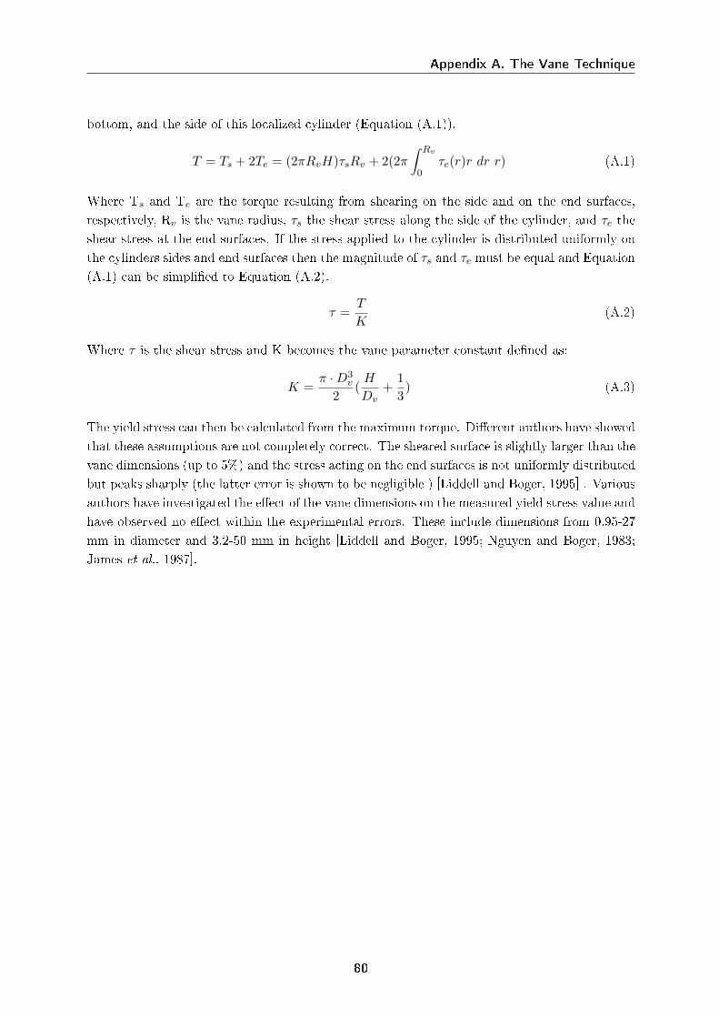
Appendix A. The Vane Technique
bottom, and the side of this localized cylinder (Equation (A.1)).
T = Ts + 2Te = (2πRvH)τsRv + 2(2π
∫ Rv
0τe(r)r dr r) (A.1)
Where Ts and Te are the torque resulting from shearing on the side and on the end surfaces,respectively, Rv is the vane radius, τs the shear stress along the side of the cylinder, and τe theshear stress at the end surfaces. If the stress applied to the cylinder is distributed uniformly onthe cylinders sides and end surfaces then the magnitude of τs and τe must be equal and Equation(A.1) can be simplied to Equation (A.2).
τ =T
K(A.2)
Where τ is the shear stress and K becomes the vane parameter constant dened as:
K =π ·D3
v
2(
H
Dv+
13) (A.3)
The yield stress can then be calculated from the maximum torque. Dierent authors have showedthat these assumptions are not completely correct. The sheared surface is slightly larger than thevane dimensions (up to 5%) and the stress acting on the end surfaces is not uniformly distributedbut peaks sharply (the latter error is shown to be negligible ) [Liddell and Boger, 1995] . Variousauthors have investigated the eect of the vane dimensions on the measured yield stress value andhave observed no eect within the experimental errors. These include dimensions from 0.95-27mm in diameter and 3.2-50 mm in height [Liddell and Boger, 1995; Nguyen and Boger, 1983;James et al., 1987].
80
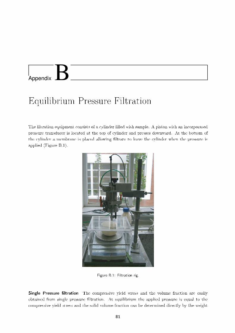
Appendix BEquilibrium Pressure Filtration
The ltration equipment consists of a cylinder lled with sample. A piston with an incorporatedpressure transducer is located at the top of cylinder and presses downward. At the bottom ofthe cylinder a membrane is placed allowing ltrate to leave the cylinder when the pressure isapplied (Figure B.1).
Figure B.1: Filtration rig.
Single Pressure ltration The compressive yield stress and the volume fraction are easilyobtained from single pressure ltration. At equilibrium the applied pressure is equal to thecompressive yield stress and the solid volume fraction can be determined directly by the weight
81
Appendix B. Equilibrium Pressure Filtration
lost and drying method or indirectly by use of Equation (B.1.) [de Kretser et al., 2005].
φf = φ0h0
hf(B.1)
Stepped Pressure ltration The smallest pressure is applied until the lter cake stops com-pressing. The pressure is then raised and the procedure repeated until all chosen pressures havebeen applied to the lter cake [Usher et al., 2001].
82
Appendix CCentrifugation
In the centrifugation technique, the sample is centrifuged until equilibrium is achieved i.e. untila steady sediment height is reached. Then the pressure at any point in the particle network canbe determined by the weight of the particles above that point (Equation (C.1)) [Miller et al.,1996].
P (z) =∫ Heq
z∆ρ g(z) φ(z) dz (C.1)
where P is the pressure acting on the particle network, z denotes the height of the given pointmeasured from the bottom of the column, Heq is the sediment height at equilibrium, ∆ρ is thedierence between the density of the solid and liquid, g(z) the centrifugal acceleration, and thesolid volume fraction is given by φ(z). The centrifugal acceleration is given:
g(z) = g0(1− z/R) (C.2)
and is determined by the acceleration at the base of the column (g0) and the distance fromthe centre of the rotor to the bottom of the column (R) [Miller et al., 1996]. The consolidationequilibrium is reached when the particle network is able to sustain the applied pressure elastically(Pyφ(z)=P(z)). Equation (C.1) can therefore be used to determine the compressive yield stress.To two most common techniques used to determine the compressive yield stress are either aconcentration prole technique where the volume fraction is measured directly or a multiple speedsediment height technique where the volume fraction is determined indirectly [Miller et al., 1996;Buscall and White, 1987].
83
Appendix C. Centrifugation
84
Appendix DSolid Concentration Calculations
The solid mass fraction (x) of a suspension can be calculated as follows:
x =mwet −mempty
mdry −mempty(D.1)
where mwet is the mass of the tray and the suspension before drying, mempty is the mass of theempty tray, and mdry is the mass of the tray and the suspension after drying.
The solid mass fraction (x) of the solution can be converted to solid volume fraction (φ) if theparticle density (ρp) and the liquid density (ρl) is known D.2.
φ =1
1 + ρp
ρl
(1x − 1
) (D.2)
Conversion from solid volume fraction (φ) to solid mass fraction (x) is as follows:
x =1
1 + ρlρp
(1φ − 1
) (D.3)
and the suspension density ρs can be calculated as follows:
ρs =1
xρp
+ (1−x)ρl
(D.4)
85

Appendix D. Solid Concentration Calculations
86
Enclosure ICalculation of the Error in using Low TorqueData from the Haake Viscometer
On the Haake viscometer the torque range is from 100-30,000 µNm ± 5% (fsd) [Rheology Solu-tions Pty Ltd, 2008] and the calculated min. and max. stesses for the dierent vanes are givenin Table I.1.
Table I.1: The stress ranges that can be measured at the Haake Viscometer with the dierent vane geometriescalculated on basis of the sensibility of torque in the instrument.
Vane min. measurable max. measurablestress [Pa] stress [Pa]
1 34.8 10,4262 5.8 1,7353 2.6 792.24 1.7 523.85 1.2 366.76 0.2 65.57 0.03 8.2
The error on the measured torque values is determined using least square linear regression onthe apparent linear part of the torque vs stress curve where the suspension yields (Figure I.1).A line is tted through the points and the dierence between the points and the tted line isdetermined.
87
Enclosure I. Calculation of the Error in using Low Torque Data from the Haake Viscometer
0 2 4 6 8 10 12 14 16 18 20
0
500
1000
1500
2000
2500
3000
Torq
ue [µN
m]
Time [s]
data points linear fit
Figure I.1: Calculation of the error on the torque for a measurement with vane 1 on a 0.36 v/v aluminasuspension.
The error is then determined by:
Error% =n∑
n=1
(M −M
M· 100%
)/n (I.1)
where M is the torque and M is the torque calculated from the linear t. The results are givenin Table I.2.
Table I.2: The dierent vane geometries and the stress ranges that can be measured at the Haake Viscometerwith each of them calculated on basis of the sensibility of the transducer/sensor? in the instrument.
φ Vane 7 Vane 6 Vane 4[-] τy [Pa] M [µNm] error [%] τy [Pa] M [µNm] error [%] τy [Pa] M [µNm] error [%]
0.169 49.3 22,600 0.44 41.0 2,300 1.290.126 18.8 8,600 0.64 11.6 670 3.180.106 8.0 29,400 0.43 7.5 3,400 1.17 4.6 260 3.520.100 6.8 24,800 0.37 6.4 2,900 1.190.095 5.6 20,500 0.48 5.1 2,300 1.220.090 4.7 17,100 0.37 4.1 1,900 1.64
From Table I.2 the dierence in shear yield stress, the measured torque, and the error on thetorque can be viewed for three dierent vanes. According to the Haake instrument manual theerror on the torque is ± 0.5% which means that the vaules measured with Vane 7 are within theaccepted error range. On basis of the data, it can then be concluded that an error≥ 1.17% onthe measured torque/stress and a torque ≤ 3,400 µNm leads to a ≥ 6% lower shear yield stressvalue. It is therefore determined that 3,400 µNm is the minimum torque valid for measuring onthe Haake. This leads to the following limits for the dierent vanes (Table I.3).
88
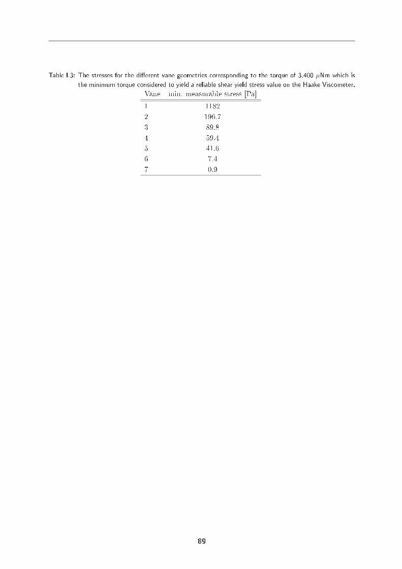
Table I.3: The stresses for the dierent vane geometries corresponding to the torque of 3,400 µNm which isthe minimum torque considered to yield a reliable shear yield stress value on the Haake Viscometer.
Vane min. measurable stress [Pa]1 11822 196.73 89.84 59.45 41.66 7.47 0.9
89
Enclosure I. Calculation of the Error in using Low Torque Data from the Haake Viscometer
90
Enclosure IICalculation of Compressive Yield Stress fromEquilibrium Batch Settling
The principle of batch settling is that a suspension is settled under gravity until equilibrium isreached. The pressure gradient (dp
dz ) is determined by the density dierence between the solidand the liquid (∆ρ), the gravitational force (g), and the volume fraction of the bed (φ):
dp
dz= −∆ρgφ (II.1)
At equilibrium the network pressure (P) acting on the bed is equal to the compressive yield stress(Py) at all heights. At initial solids concentrations below the gel point (φ0<φg) the networkpressure at the top of the bed is zero while that at the base, due to the overlying suspension isdetermined according to:
Pz=0 = ∆ρgφ0h0 (II.2)
where ∆ρ is the dierence in density between the solid and liquid, g is the gravitational force, andh0 is the initial sample height. Employing the end conditions, Equation (II.1) can be integratedto yield:
∫ hf
0dz =
1∆ρg
∫ 0
∆ρgφ0h0
−1φ
dp ⇒ hf =h0φ0
φ(II.3)
As Equation (II.3) is employed to calculate the average solid volume concentration, the averagePy can be calculated as Pz=0/2.
Five batch settling tests were performed by employing a xed initial volume fraction and dierentinitial heights. The samples were left to settle for 86 days. By viewing the nal height as afunction of log time it can be determined whether equilibrium has been reached (Figure II.1).
91
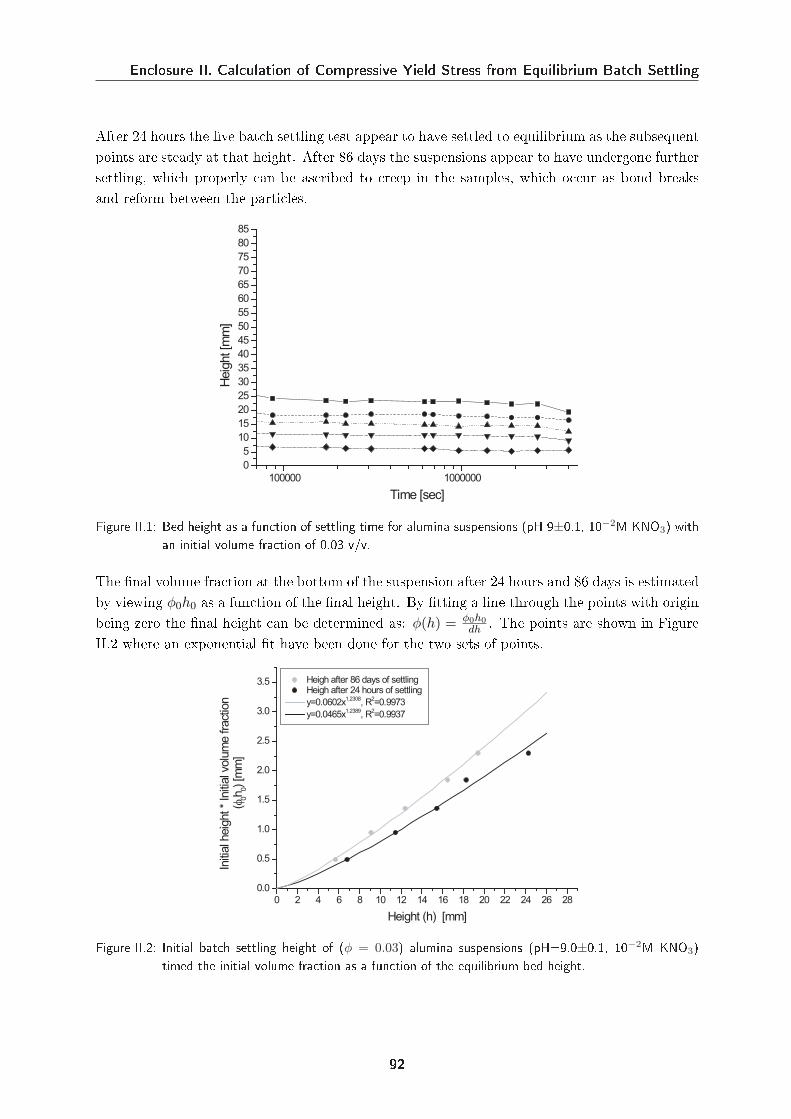
Enclosure II. Calculation of Compressive Yield Stress from Equilibrium Batch Settling
After 24 hours the ve batch settling test appear to have settled to equilibrium as the subsequentpoints are steady at that height. After 86 days the suspensions appear to have undergone furthersettling, which properly can be ascribed to creep in the samples, which occur as bond breaksand reform between the particles.
100000 1000000
0
5
10
15
20
25
30
35
40
45
50
55
60
65
70
75
80
85H
eig
ht [m
m]
Time [sec]
Figure II.1: Bed height as a function of settling time for alumina suspensions (pH 9±0.1, 10−2M KNO3) withan initial volume fraction of 0.03 v/v.
The nal volume fraction at the bottom of the suspension after 24 hours and 86 days is estimatedby viewing φ0h0 as a function of the nal height. By tting a line through the points with originbeing zero the nal height can be determined as: φ(h) = φ0h0
dh . The points are shown in FigureII.2 where an exponential t have been done for the two sets of points.
0 2 4 6 8 10 12 14 16 18 20 22 24 26 28
0.0
0.5
1.0
1.5
2.0
2.5
3.0
3.5
Initi
al h
eig
ht *
Initi
al v
olu
me fra
ctio
n (φ 0
h0)
[m
m]
Height (h) [mm]
Heigh after 86 days of settling Heigh after 24 hours of settling
y=0.0602x1.2308
, R2=0.9973
y=0.0465x1.2389
, R2=0.9937
Figure II.2: Initial batch settling height of (φ = 0.03) alumina suspensions (pH=9.0±0.1, 10−2M KNO3)timed the initial volume fraction as a function of the equilibrium bed height.
92
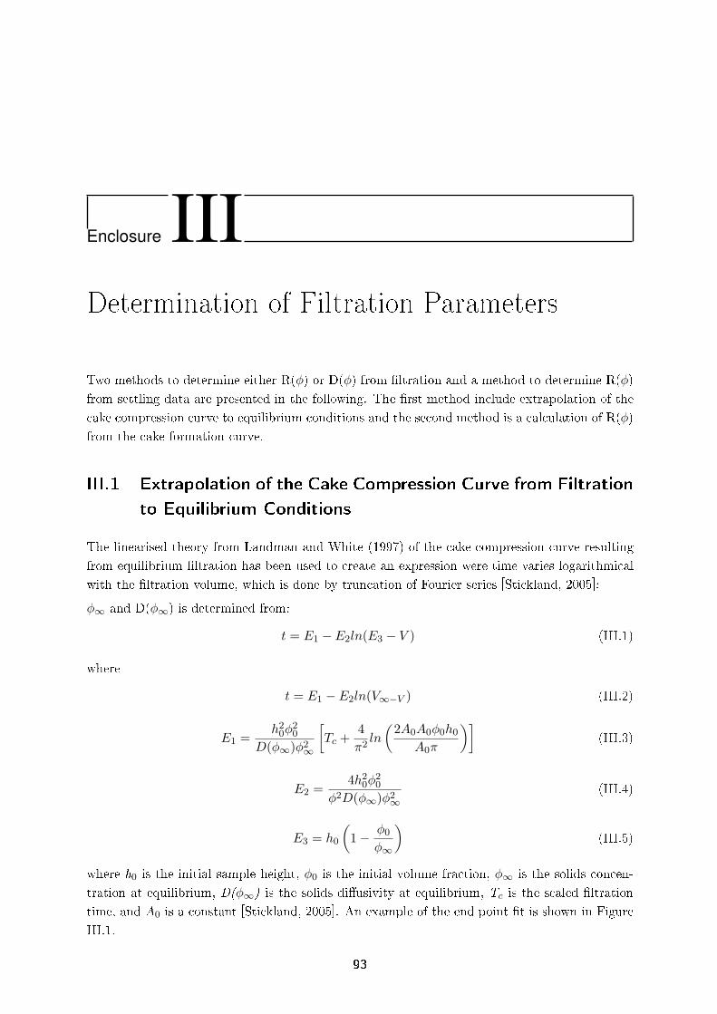
Enclosure IIIDetermination of Filtration Parameters
Two methods to determine either R(φ) or D(φ) from ltration and a method to determine R(φ)from settling data are presented in the following. The rst method include extrapolation of thecake compression curve to equilibrium conditions and the second method is a calculation of R(φ)from the cake formation curve.
III.1 Extrapolation of the Cake Compression Curve from Filtrationto Equilibrium Conditions
The linearised theory from Landman and White (1997) of the cake compression curve resultingfrom equilibrium ltration has been used to create an expression were time varies logarithmicalwith the ltration volume, which is done by truncation of Fourier series [Stickland, 2005]:φ∞ and D(φ∞) is determined from:
t = E1 −E2ln(E3 − V ) (III.1)
where
t = E1 − E2ln(V∞−V ) (III.2)
E1 =h2
0φ20
D(φ∞)φ2∞
[Tc +
4π2
ln
(2A0A0φ0h0
A0π
)](III.3)
E2 =4h2
0φ20
φ2D(φ∞)φ2∞(III.4)
E3 = h0
(1− φ0
φ∞
)(III.5)
where h0 is the initial sample height, φ0 is the initial volume fraction, φ∞ is the solids concen-tration at equilibrium, D(φ∞) is the solids diusivity at equilibrium, Tc is the scaled ltrationtime, and A0 is a constant [Stickland, 2005]. An example of the end point t is shown in FigureIII.1.
93
Enclosure III. Determination of Filtration Parameters
Figure III.1: Example of end point t from extrapolation of the cake formation region to yield φ∞ and D(φ∞)[Stickland, 2005].
III.2 Hindered Settling Function From the Cake Formation Filtra-tion Curve
The hindered settling function, R(φ), is related to the specic cake resistance, α:
α =R(φ)
(1− φ)2ρsη(III.6)
where ρs is the solids density and η is the ltrate viscosity.From the traditional Ruth/Darcian ltration equation, which assumes a linear cake formationregion, the specic cake resistance can be determined;
αav =2∆P
ηρs
(1φ0− 1
φc
)· δ(t/V )
δV(III.7)
where ∆ P is the pressure dierence, ρs is the solids density, η is the ltrate viscosity, φ0 isthe initial volume fraction, and φc is the average solids concentration in the cake. CombiningEquation (III.6) and (III.7):
R(φc) = 2∆P (1− φc)2(
1φ0− 1
φc
)· δ(t/V )
δV(III.8)
III.3 Hindered Settling Function From the Batch Settling
The hindered settling function below the gel point can be determined from batch settling exper-iments. Lester et al. (2005) developed a method for determining hindered settling function data
94
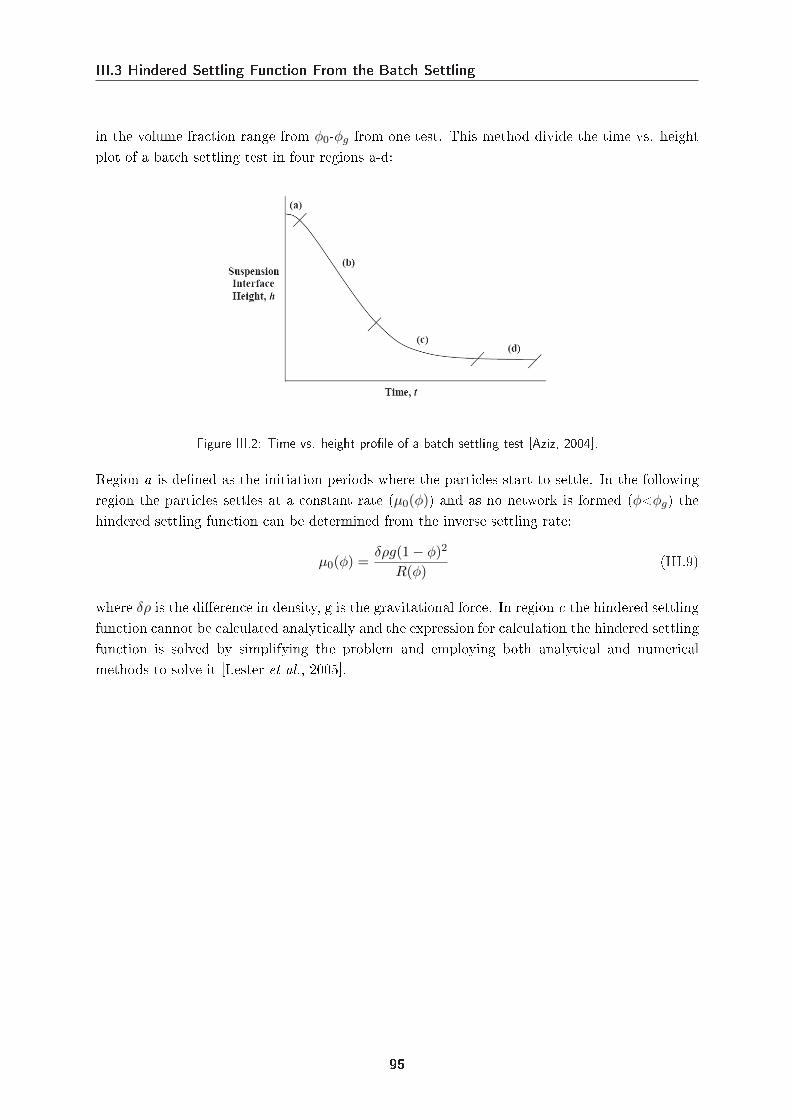
III.3 Hindered Settling Function From the Batch Settling
in the volume fraction range from φ0-φg from one test. This method divide the time vs. heightplot of a batch settling test in four regions a-d:
Figure III.2: Time vs. height prole of a batch settling test [Aziz, 2004].
Region a is dened as the initiation periods where the particles start to settle. In the followingregion the particles settles at a constant rate (µ0(φ)) and as no network is formed (φ<φg) thehindered settling function can be determined from the inverse settling rate:
µ0(φ) =δρg(1− φ)2
R(φ)(III.9)
where δρ is the dierence in density, g is the gravitational force. In region c the hindered settlingfunction cannot be calculated analytically and the expression for calculation the hindered settlingfunction is solved by simplifying the problem and employing both analytical and numericalmethods to solve it [Lester et al., 2005].
95