Option Anatomy

Copenhagen University

March 2013

Jesper Andreasen

Danske Markets, Copenhagen

kwant.daddy@danskebank.com

2

Outline

Acknowledgements.

Kwant life.

Introduction.

Volatility interpolation.

Wots me Δelδa?

Conclusion.

3

References

Andreasen, J and B Huge (2011a): “Volatility Interpolation.” Risk March,

76-79.

Andreasen, J and B Huge (2011b): “Random Grids.” Risk July, 66-71.

Andreasen, J and B Huge (2013a): “Expanding Forward Volatility.” Risk

January, 104-107.

Andreasen, J and B Huge (2013b): “Wots me Δelδa?” Unfinished wp,

Danske Markets.

Balland, P (2006): “Forward Smile.” Presentation, ICBI Global Derivatives.

Carr, P. (2008): “Local Variance Gamma.” WP, Bloomberg.

4

Dupire, B (1994): “Pricing with a Smile.” Risk January, 18-20.

Dupire, B (2006): “Skew Modeling.” Presentation, ICBI Global Derivatives.

Hagan, P, D Kumar, A Lesniewski, D Woodward (2002). “Managing Smile

Risk.” Wilmott Magazine September, 84-108.

Nabben, R. (1999): “On Decay Rates of Tridiagonal and Band Matrices.”

SIAM J. Matrix Anal. Appl. 20, 820-837.

5

Thanks to ...

Copenhagen University and the scientific committee (Rolf Poulsen, Michael

Sørensen, Mogens Steffensen) for awarding me the title of Adjungeret

Professor in Mathematical Finance at the Department of Mathematics.

The many great colleagues that I have had the pleasure and privilege to work

with over the past 16 years. Not least co-authors Leif Andersen and Brian

Huge.

The great teachers and mentors: Maria Arys, Jørgen Aase Nielsen, and

William Keirstead.

6

Kwant Life

In the late 90s and early 00s the main focus of quant work was the pricing of

ever more complicated products and pay-offs.

The general approach was to take the vanillas as direct inputs and focus the

modelling of the exotics.

The financial crisis (luckily) changed that. Liquidity dried up and the model

focus over the past 5 years has been much more fundamental.

Particularly, a lot of quant energy has gone into answering the questions:

- What is the forward? Libor basis ...

- How to discount? X-ccy basis, collateral, xVA, ...

7

In fact, quant technology is more in demand and in wide spread use today,

than it ever was.

Quant clients have been extended to include the whole universe of

derivatives trading and more.

In this talk, we are going to consider the next step up in complexity from

forwards and discounting:

- How to price and hedge an option?

8

Introduction

Andreasen and Huge won the Risk Magazine Quant of the Year 2012 award

for the two papers Volatility Interpolation and Random Grids.

“...The pair turned conventional approaches on their head, to the bafflement

of their colleagues in the quant community, with some highly original

thinking on the subject of implied volatility calibration...”

I could not have said it better myself.

The general idea is to work directly with discrete finite difference based

models rather than with the continuous time stochastic differential equations.

9

The focus is on stability, computer implementation, and consistency with

market quotes, rather than perceived accuracy relative to some theoretical

stochastic differential equations.

...which are irrelevant because the discrete model is calibrated to market

quotes.

The idea can be applied to other types of approximations than the finite

difference method.

Specifically, we have over the past 3-4 years worked a lot on expansions

used on their own or in combination with finite difference methods.

Today, we will consider two very fundamental problems:

- How to interpolate discrete option quotes without introducing arbitrage?

10

- What Delta should I use to hedge an option?

For the first problem we will use finite difference machinery and for the

second, short maturity expansions.

Note: This is a very compressed presentation where we omit a (large)

number of proofs, technicalities, extensions, applications, references, and

deeper thoughts.

11

Volatility Interpolation

Someone said that the Black-Scholes formula is the wrong formula

ln / 1( , ) ( ) ( ) ,

2s kc t k s k v t

v t (1)

...but if you stuff in a wrong number, for the (implied) volatility v , then you

might get the right option price.

Suppose you have a discrete set of implied volatilities

( , ) , 1, ,i i

v t k i n (2)

... corresponding to the discrete set of option prices 1, ,

{ ( , )}i i i n

c t k .

12

It seems like a trivial exercise to interpolate and extrapolate these implied

volatilities into a continuous surface of option prices in expiry and strike

0, 0{ ( , )}

t kc t k ...

... except that it very much isn’t!

The trouble is that it exceptionally easy to break the arbitrage conditions

2

2

( , ) ( , )0 , 0c t k c t kt k

(3)

For a given interpolation scheme for the implied volatilities one can compute

the resulting surface of forward volatilities using Dupire’s forward volatility

formula:

13

22

21( ) 0 [ ( ) | ( ) ]2

c cds t dW E t s t kt k

(4)

The point here is that if the arbitrage conditions (3) are broken then the

forward volatility surface produced by (4) will have spikes and imaginary

values.

14

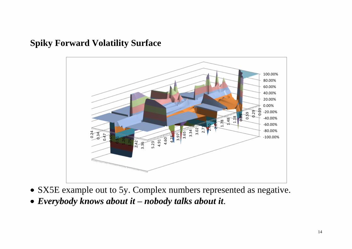
Spiky Forward Volatility Surface

SX5E example out to 5y. Complex numbers represented as negative.

Everybody knows about it – nobody talks about it.

0.2

4

0.3

4

0.4

7

0.6

5

0.9

1

1.2

6

1.7

5

2.4

2

3.3

6

-100.00%

-80.00%

-60.00%

-40.00%

-20.00%

0.00%

20.00%

40.00%

60.00%

80.00%

100.00%

0.0

3

0.2

9

0.5

9

0.8

9

1.1

8

1.4

8

1.7

8

2.0

9

2.4

0

2.7

1

3.0

2

3.3

4

3.6

5

3.9

7

4.2

8

4.6

0

4.9

1

5.2

3

15

Arbitrage in the Interpolated Option Prices

Spikes in the forward volatility surface is a problem for a number of reasons:

- Forward volatility models for exotics will not work.

- Forward volatility information is distorted and useless => forward

volatility is not used in the same way as forward rates.

- Problems in risk management of options and particularly spreads.

- The risk of arbitrages in prices shown to clients => wider bid/offers.

The problem has been unresolved for nearly 20 years. Personally, I have

thinking about an efficient solution for more than 15 years.

16

Surprisingly, the solution comes from discrete math and matrix algebra and

not from a Stiefel Manifolds, Malliavin calculus, Varadhan’s lemma, or

general relativity.

Maybe that is why it has been overlooked...

17

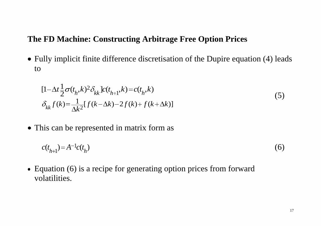
The FD Machine: Constructing Arbitrage Free Option Prices

Fully implicit finite difference discretisation of the Dupire equation (4) leads

to

2

21

1( ) [ ( ) 2 ( ) ( )]

1[1 ( , ) ] ( , ) ( , )2

kk

h kk h h

f k f k k f k f k kk

t t k c t k c t k (5)

This can be represented in matrix form as

1

1( ) ( )

h hc t A c t (6)

Equation (6) is a recipe for generating option prices from forward

volatilities.

18

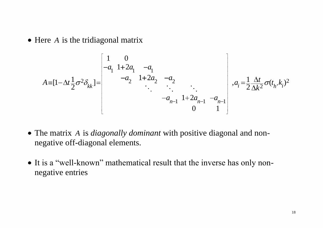
Here A is the tridiagonal matrix

1 1 1

2 22 2 2 ,2

1 1 1

1 01 2

1 21 1[1 ] , ( )2 2

1 2

0 1

i ikk h

n n n

a a a

a a a tA t a t kk

a a a

The matrix A is diagonally dominant with positive diagonal and non-

negative off-diagonal elements.

It is a “well-known” mathematical result that the inverse has only non-

negative entries

19

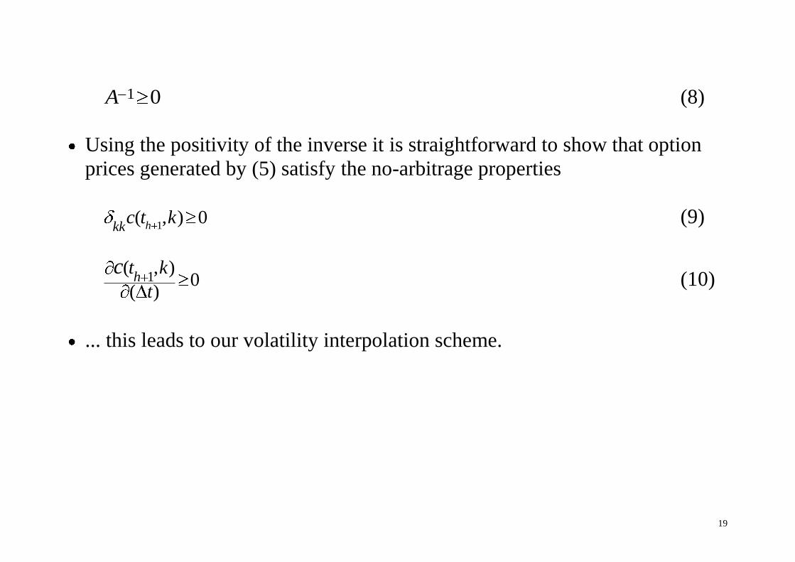
1 0A (8)

Using the positivity of the inverse it is straightforward to show that option

prices generated by (5) satisfy the no-arbitrage properties

1( , ) 0

hkkc t k (9)

1( , )

0( )h

t k

t

c (10)

... this leads to our volatility interpolation scheme.

20

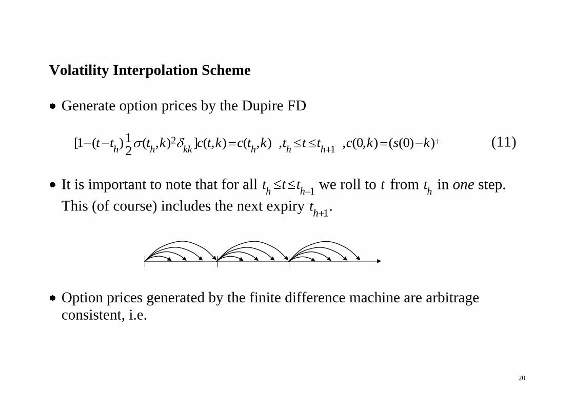
Volatility Interpolation Scheme

Generate option prices by the Dupire FD

2

11[1 ( ) ( , ) ] ( , ) ( , ) , , (0, ) ( (0) )2h h kk h h h

t t t k c t k c t k t t t c k s k (11)

It is important to note that for all 1h h

t t t we roll to t from h

t in one step.

This (of course) includes the next expiry 1h

t .

Option prices generated by the finite difference machine are arbitrage

consistent, i.e.

21

2

20 0 0 ( , )c c c t k

t kk (12)

22

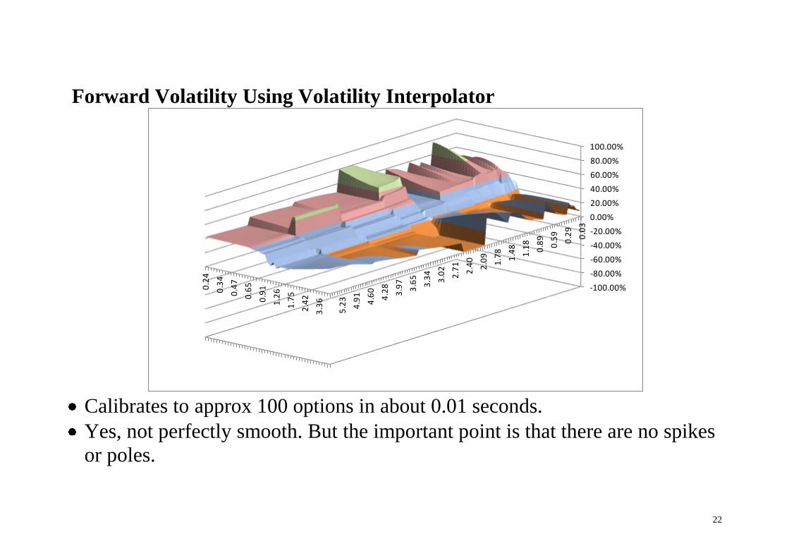
Forward Volatility Using Volatility Interpolator

Calibrates to approx 100 options in about 0.01 seconds.

Yes, not perfectly smooth. But the important point is that there are no spikes

or poles.

0.2

4

0.3

4

0.4

7

0.6

5

0.9

1

1.2

6

1.7

5

2.4

2

3.3

6

-100.00%

-80.00%

-60.00%

-40.00%

-20.00%

0.00%

20.00%

40.00%

60.00%

80.00%

100.00%

0.0

3

0.2

9

0.5

9

0.8

9

1.1

8

1.4

8

1.7

8

2.0

9

2.4

0

2.7

1

3.0

2

3.3

4

3.6

5

3.9

7

4.2

8

4.6

0

4.9

1

5.2

3

23

Nuclear Submarines

In the 50s, USA and CCCP competed in being the first to put a nuclear

reactor inside a submarine.

One of the main difficulties in doing so is to dimension the cooling system

accurately: not too big and not too small.

For the related calculations on the heat equation (the Black-Scholes PDE),

the Americans used the Crank-Nicolson method.

...whereas the Russians used the fully implicit method. Like we do.

The CN method is superior in terms speed of convergence but its solution

exhibits small oscillations.

24

The fully implicit method shows slower convergence but it has no

oscillations.

If you have a good computer you will use Crank-Nicolson, and that is what

we have been taught to do in skool.

But if your computer is a bunch of class enemies sitting in Siberia,

...or if you need to calibrate the parameters of your finite difference grid to

observed option prices,

... then the stability matters more than (theoretical) speed of convergence and

you will use the fully implicit method.

25

Wots me Δelδa?

It’s the most pressing question for any option trader.

The quant’s standard answer is:

“That depends on the model -- and I have ten of them, you pick one...”

Hagan et al (2002) argues that the delta can be fine tuned in stochastic local

volatility models by changing the correlation versus the local volatility

component – when the volatility smile is kept the same.

Dupire (2006), however, counters that and argues that close to ATM, the

minimum variance delta is virtually invariant to the choice of correlation

versus local volatility – when the smile is kept the same.

26

The minimum variance delta is the position in the underlying stock that

(locally) hedges as much variance of the option, i.e. including volatility risk,

as possible:

cov[ , ]

var[ ]s vdv dsc c

ds (13)

Here we provide a general proof of Dupire’s statement in the context of

short maturity expansions.

We then show that a model free MV gamma also can be produced, and that

the ATM theta as well as behaviour of away from ATM can be linked to the

value of options on volatility.

27

Short Maturity Expansion

Consider the following (very) general class of stochastic volatility model

( , )

( , )

( , )

ds s z dW

dz s z dZ

dW dZ s z dt

(14)

Clearly the family of models (14) is rich enough to include several models

that fit the same smile.

As an example, one can think of the smile generated by a Heston model but

fitted by a pure local volatility model.

Let ( )c t be the time t price of a European option on s . Suppose we write the

option price as

28

( ) ( , ( ), ( ))c t g t s t v t (15)

... where ( )g is Bachelier’s option price formula and v is the implied normal

volatility. I.e.

( , , ) ( ) ( ) ( ) , ,x x s kg t s v s k v x T tv (16)

Ito expansion of the option price ( , , )c g t s v yields the following arbitrage

condition on the implied volatility

20 ( ) 2 [ ]tdx dt E dvv (17)

As 0 we get the condition that x needs to be of unit diffusion, i.e.

29

22 2 2 22 1 , ( ) 0z zs s

dx x x x x x s kdt

(18)

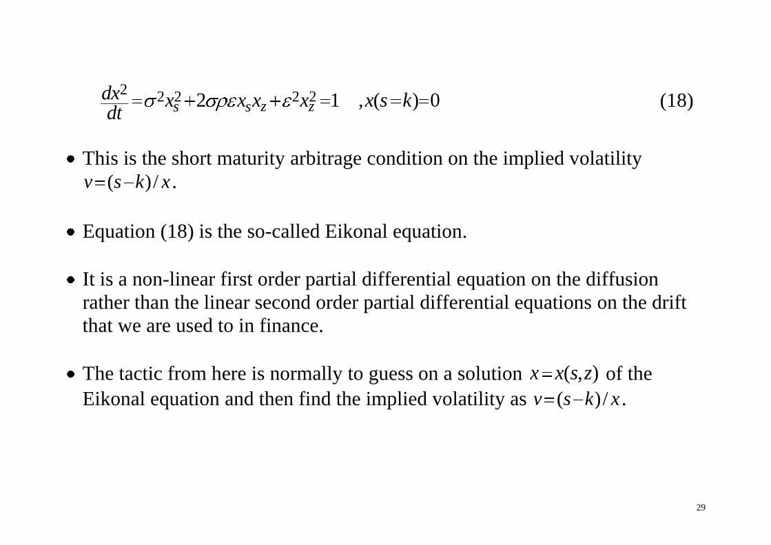
This is the short maturity arbitrage condition on the implied volatility

( )/v s k x .

Equation (18) is the so-called Eikonal equation.

It is a non-linear first order partial differential equation on the diffusion

rather than the linear second order partial differential equations on the drift

that we are used to in finance.

The tactic from here is normally to guess on a solution ( , )x x s z of the

Eikonal equation and then find the implied volatility as ( )/v s k x .

30

The short maturity expansions are (generally) not sufficiently accurate for

calibration of dynamic models.

But they are generally robust and can be used for market making of an

option book and/or for gaining intuition about the qualitative effect of

various model parameters.

Well-known examples include the so-called SABR model.

Rather than deriving new pricing equations, the aim here is come up with

general asymptotic results for the Greeks, at and around ATM that are valid

for all models hitting the initial smile.

31

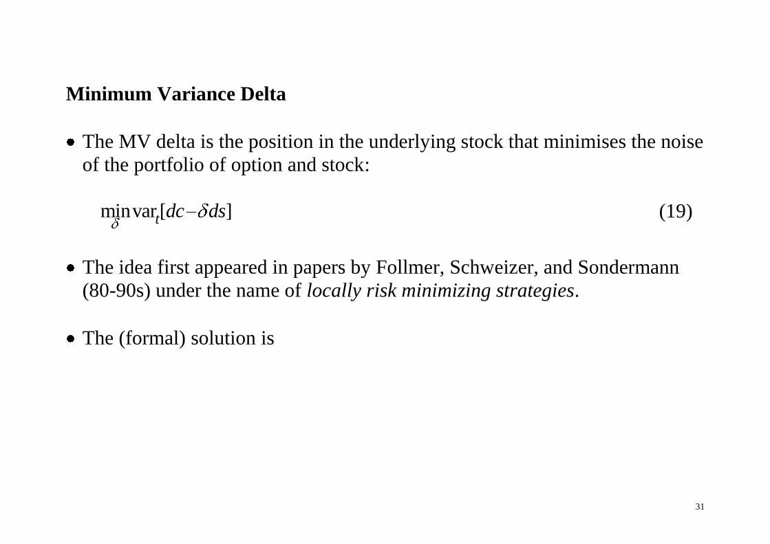
Minimum Variance Delta

The MV delta is the position in the underlying stock that minimises the noise

of the portfolio of option and stock:

minvar [ ]t dc ds (19)

The idea first appeared in papers by Follmer, Schweizer, and Sondermann

(80-90s) under the name of locally risk minimizing strategies.

The (formal) solution is

32

minvar

[ ]z zs s v sveganaive stickycorrection deltaofdelta strikeforvolcorr theimplied vol

delta

onlydepend onsmile

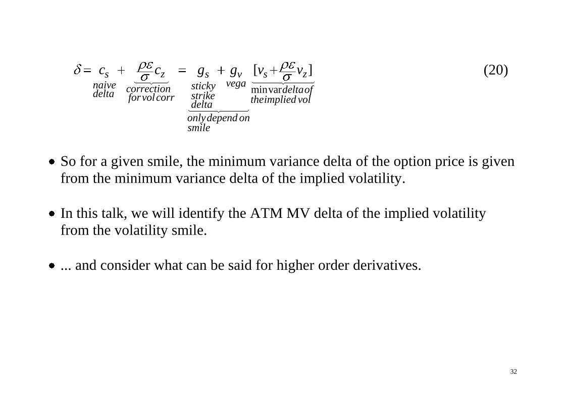
c c g g v v (20)

So for a given smile, the minimum variance delta of the option price is given

from the minimum variance delta of the implied volatility.

In this talk, we will identify the ATM MV delta of the implied volatility

from the volatility smile.

... and consider what can be said for higher order derivatives.

33

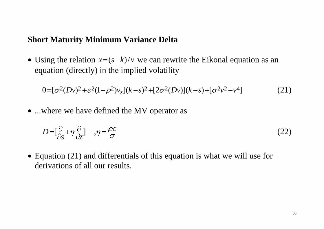
Short Maturity Minimum Variance Delta

Using the relation ( )/x s k v we can rewrite the Eikonal equation as an

equation (directly) in the implied volatility

2 2 2 2 2 2 2 2 40 [ ( ) (1 ) ]( ) [2 ( )]( ) [ ]zDv v k s Dv k s v v (21)

...where we have defined the MV operator as

[ ] ,Ds z

(22)

Equation (21) and differentials of this equation is what we will use for

derivations of all our results.

34

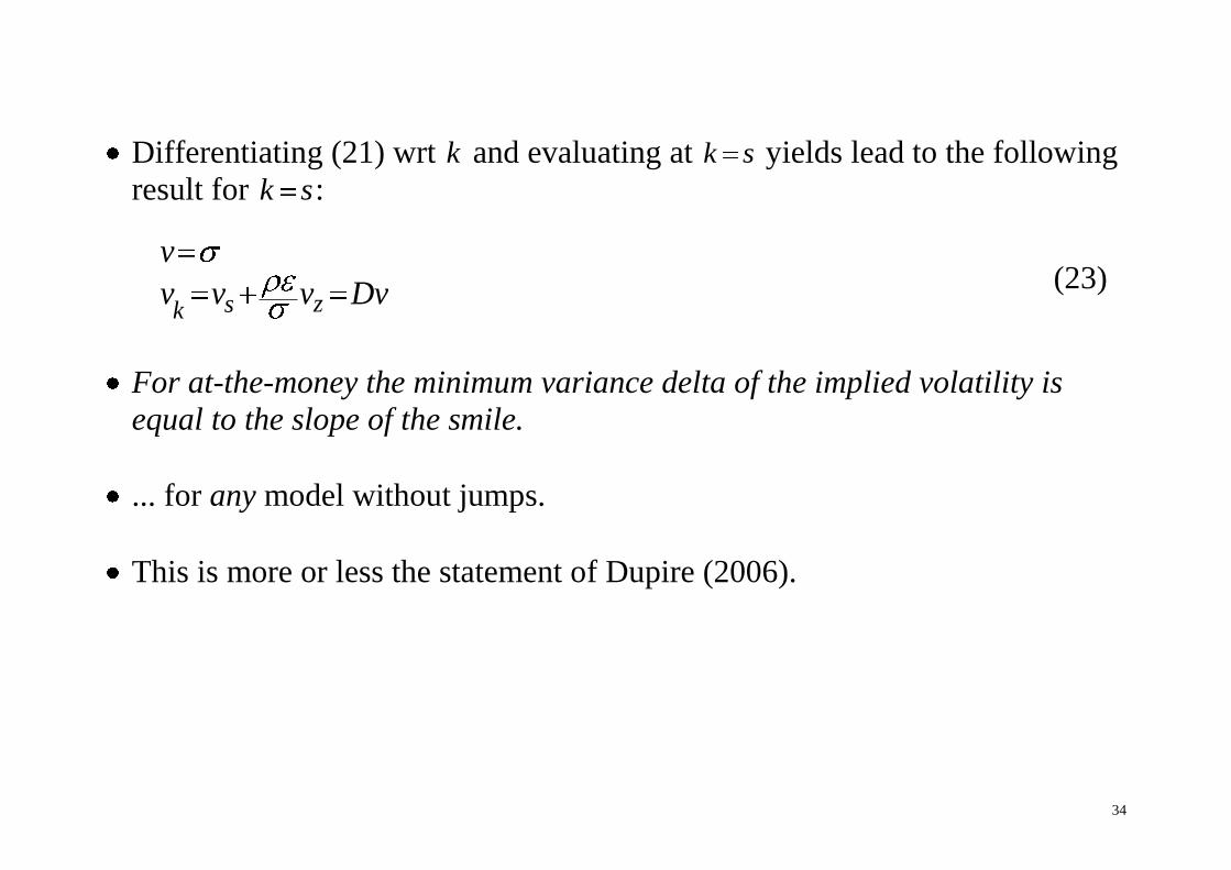
Differentiating (21) wrt k and evaluating at k s yields lead to the following

result for k s:

zsk

v

v v v Dv (23)

For at-the-money the minimum variance delta of the implied volatility is

equal to the slope of the smile.

... for any model without jumps.

This is more or less the statement of Dupire (2006).

35

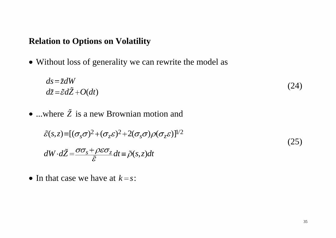
Relation to Options on Volatility

Without loss of generality we can rewrite the model as

( )

ds zdW

dz dZ O dt (24)

...where Z is a new Brownian motion and

2 2 1/2( , ) [( ) ( ) 2( ) ( )]

( , )

z zs s

zs

s z

dW dZ dt s z dt

(25)

In that case we have at k s:

36

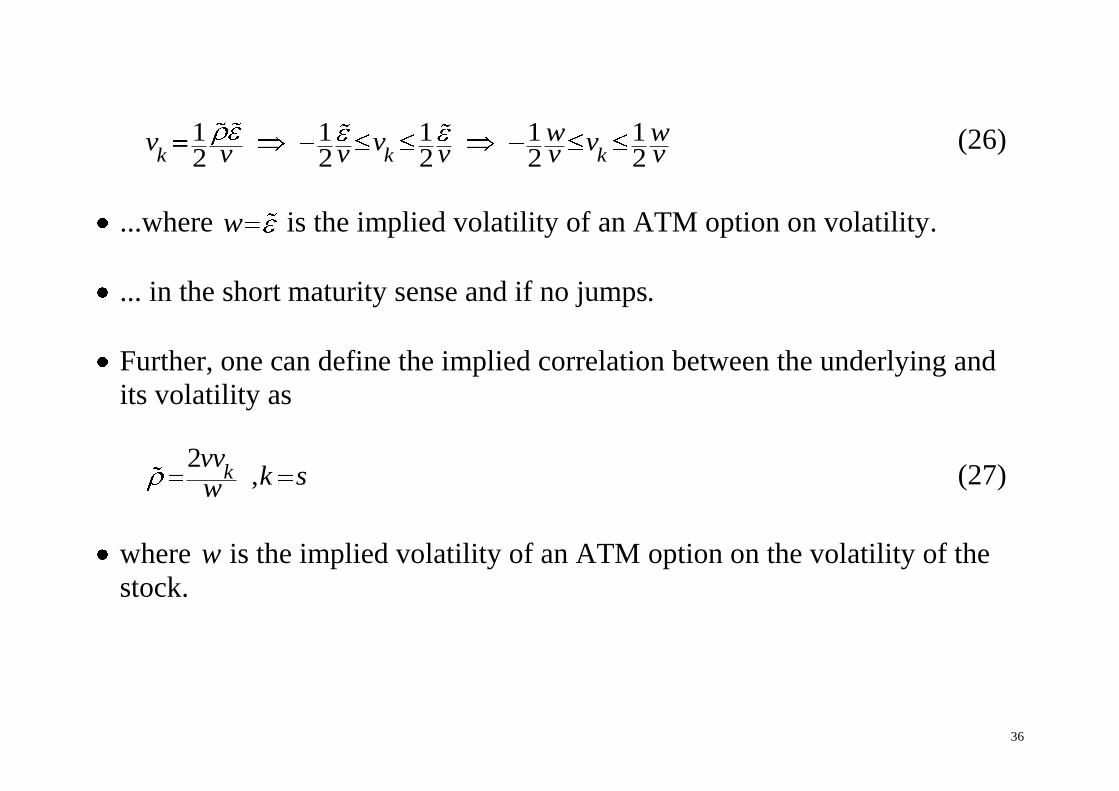
1 1 1 1 12 2 2 2 2k k k

w wv v vv v v v v (26)

...where w is the implied volatility of an ATM option on volatility.

... in the short maturity sense and if no jumps.

Further, one can define the implied correlation between the underlying and

its volatility as

2

,kvv

k sw (27)

where w is the implied volatility of an ATM option on the volatility of the

stock.

37

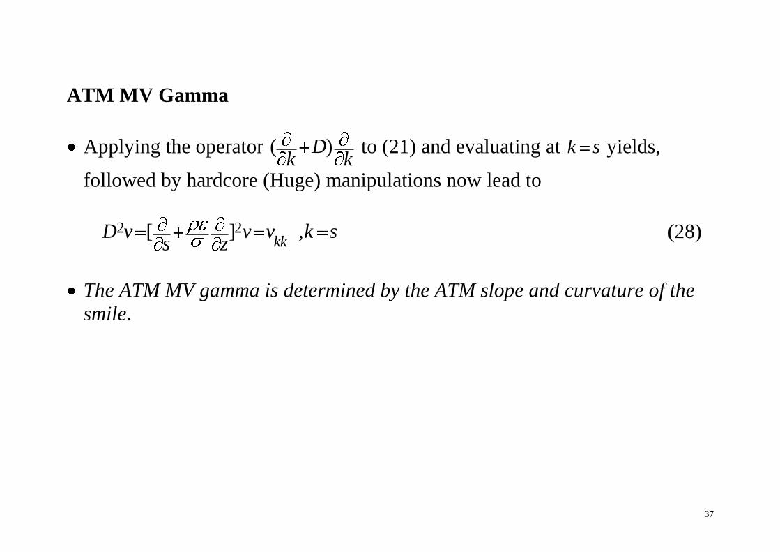
ATM MV Gamma

Applying the operator ( )Dk k

to (21) and evaluating at k s yields,

followed by hardcore (Huge) manipulations now lead to

2 2[ ] ,

kkD v v v k s

s z (28)

The ATM MV gamma is determined by the ATM slope and curvature of the

smile.

38

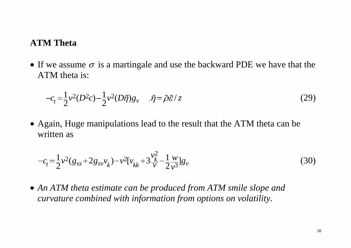
ATM Theta

If we assume is a martingale and use the backward PDE we have that the

ATM theta is:

,2 2 21 1( ) ( )2 2

/vtc v D c v D g z (29)

Again, Huge manipulations lead to the result that the ATM theta can be

written as

2

2 23

1 1( 2 ) [ 3 ]2 2

kss sv vt k kk

v wc v g g v v v gv v (30)

An ATM theta estimate can be produced from ATM smile slope and

curvature combined with information from options on volatility.

39

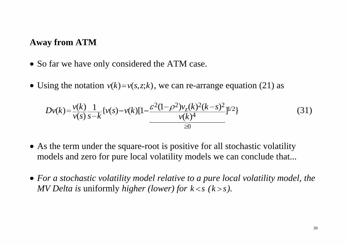
Away from ATM

So far we have only considered the ATM case.

Using the notation ( ) ( , ; )v k v s z k , we can re-arrange equation (21) as

2 2 2 2

1/24

0

(1 ) ( ) ( )( ) 1( ) { ( ) ( )[1 ] }( ) ( )

zv k k sv kDv k v s v kv s s k v k

(31)

As the term under the square-root is positive for all stochastic volatility

models and zero for pure local volatility models we can conclude that...

For a stochastic volatility model relative to a pure local volatility model, the

MV Delta is uniformly higher (lower) for k s (k s).

40

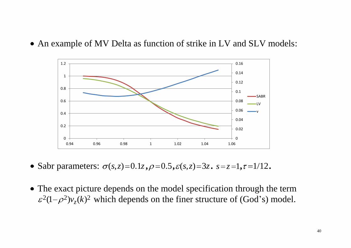
An example of MV Delta as function of strike in LV and SLV models:

Sabr parameters: ( , ) 0.1s z z , 0.5, ( , ) 3s z z . 1s z , 1/12.

The exact picture depends on the model specification through the term 2 2 2(1 ) ( )zv k which depends on the finer structure of (God’s) model.

0

0.02

0.04

0.06

0.08

0.1

0.12

0.14

0.16

0

0.2

0.4

0.6

0.8

1

1.2

0.94 0.96 0.98 1 1.02 1.04 1.06

SABR

LV

v

41

Conclusion

The Russian finite difference machine is an effective way for interpolation of

discrete option price quotes.

It allows for the use of forward volatility as a tool of spotting value and

mispricing in specific option quotes and volatility smiles.

The can also be used for constructing very stable dynamic models for exotic

options. See Andreasen and Huge (2011b).

The approach can be further refined using expansion as in Andreasen and

Huge (2013a) to give parametric control over the extrapolation of the wings

and smile dynamics.

42

We have produced model free short maturity limits of

- ATM minimum variance delta and gamma.

If we add in the implied volatility of an ATM option on volatility we can

also produce

- ATM Theta.

MV delta is always higher (lower) for low (high) strikes in stochastic

volatility models than in local volatility models.

Future research:

- Identify trading strategies that lock in the ATM MV Delta.

- Quantify the effect of jumps.