
Clinical Biochemistry - Lecture 6 Investigation of renal ...
Experimental Investigation of theReactions 25Mg(α,n)28Si,
26Mg(α,n)29Si, 18O(α,n)21Neand their Impact on Stellar
Nucleosynthesis
Dissertationzur Erlangung des Grades
Doktor der Naturwissenschaften
am Fachbereich Physik, Mathematik und Informatik derJohannes Gutenberg-Universitat Mainz
vorgelegt von
Sascha Falahatgeboren in Mainz am Rhein
Mainz, den 10. Juni 2010.
Max-Planck-Institut fur Chemie, Johannes Joachim Becher Weg 27, 55128 MainzInstitut fur Physik, Staudingerweg 7, 55128 Mainz


Meinen Eltern und Meinem Bruder Saman

Zusammenfassung
In der vorliegenden Dissertation werden die Kernreaktionen 25Mg(α,n)28Si, 26Mg(α,n)29Siund 18O(α,n)21Ne im astrophysikalisch interessanten Energiebereich von Eα = 1000 keVbis Eα = 2450 keV untersucht.Die Experimente wurden am Nuclear Structure Laboratory der University of Notre Dame(USA) mit dem vor Ort befindlichen Van-de-Graaff Beschleuniger KN durchgefuhrt. Hier-bei wurden Festkorpertargets mit evaporiertem Magnesium oder anodisiertem Sauerstoffmit α-Teilchen beschossen und die freigesetzten Neutronen untersucht. Zum Nachweis derfreigesetzten Neutronen wurde mit Hilfe von Computersimulationen ein Neutrondetek-tor basierend auf 3He-Zahlrohren konstruiert. Weiterhin wurden aufgrund des verstarktenAuftretens von Hintergrundreaktionen verschiedene Methoden zur Datenanalyse angewen-det. Abschliessend wird mit Hilfe von Netzwerkrechnungen der Einfluss der Reaktionen25Mg(α,n)28Si, 26Mg(α,n)29Si und 18O(α,n)21Ne auf die stellare Nukleosynthese unter-sucht.


Abstract
In the present dissertation, the nuclear reactions 25Mg(α,n)28Si, 26Mg(α,n)29Si and18O(α,n)21Ne are investigated in the astrophysically interesting energy region fromEα = 1000 keV to Eα = 2450 keV.The experiments were performed at the Nuclear Structure Laboratory of the University ofNotre Dame (USA) with the Van-de-Graaff accelerator KN. Solid state targets with evap-orated magnesium or anodized oxygen were bombarded with α-particles and the releasedneutrons detected. For the detection of the released neutrons, computational simulationswere used to construct a neutron detector based on 3He counters. Because of the strongoccurrence of background reactions, different methods of data analysis were employed.Finally, the impact of the reactions 25Mg(α,n)28Si, 26Mg(α,n)29Si and 18O(α,n)21Ne onstellar nucleosynthesis is investigated by means of network calculations.


Contents
Zusammenfassung i
Abstract iii
Contents v
List of Figures viii
List of Tables xi
1 Introduction 1
2 Nucleosynthesis in Stars 3
2.1 The Classical S-Process . . . . . . . . . . . . . . . . . . . . . . . . . . . . . 52.1.1 S-Process Branchings . . . . . . . . . . . . . . . . . . . . . . . . . . 7
2.2 Stellar Sites for the S-Process . . . . . . . . . . . . . . . . . . . . . . . . . . 92.2.1 AGB Stars . . . . . . . . . . . . . . . . . . . . . . . . . . . . . . . . 9
2.2.2 Massive Stars . . . . . . . . . . . . . . . . . . . . . . . . . . . . . . . 102.3 Nuclear Physics behind Nucleosynthesis . . . . . . . . . . . . . . . . . . . . 12
2.3.1 The Astrophysical S-Factor . . . . . . . . . . . . . . . . . . . . . . . 13
2.4 Reaction Networks . . . . . . . . . . . . . . . . . . . . . . . . . . . . . . . . 152.5 Observational Evidence - Meteoritic Grains . . . . . . . . . . . . . . . . . . 16
3 Previous Results 17
3.1 25Mg(α,n)28Si & 26Mg(α,n)29Si . . . . . . . . . . . . . . . . . . . . . . . . . 183.2 18O(α,n)21Ne . . . . . . . . . . . . . . . . . . . . . . . . . . . . . . . . . . . 27
4 Experimental Techniques and Procedures 31
4.1 The KN Accelerator and Beam Transport System . . . . . . . . . . . . . . . 324.1.1 RBS Beamline . . . . . . . . . . . . . . . . . . . . . . . . . . . . . . 32
4.1.2 0 Beamline . . . . . . . . . . . . . . . . . . . . . . . . . . . . . . . . 344.2 Neutron Detection . . . . . . . . . . . . . . . . . . . . . . . . . . . . . . . . 35
4.2.1 Moderation of Neutrons . . . . . . . . . . . . . . . . . . . . . . . . . 364.2.2 Design Principles . . . . . . . . . . . . . . . . . . . . . . . . . . . . . 36
4.2.3 Computational Simulations . . . . . . . . . . . . . . . . . . . . . . . 374.2.4 Parameter Studies . . . . . . . . . . . . . . . . . . . . . . . . . . . . 40
4.2.5 Design of the Test Detector . . . . . . . . . . . . . . . . . . . . . . . 434.3 Neutron Detector Construction . . . . . . . . . . . . . . . . . . . . . . . . . 46
4.3.1 Electronics Setup of the Neutron Detectors . . . . . . . . . . . . . . 50
vi CONTENTS
4.3.2 Validation of Computational Calculations . . . . . . . . . . . . . . . 50
4.4 Counting Station . . . . . . . . . . . . . . . . . . . . . . . . . . . . . . . . . 52
4.5 (p,γ)-Measurement Setup . . . . . . . . . . . . . . . . . . . . . . . . . . . . 52
4.6 Target Production . . . . . . . . . . . . . . . . . . . . . . . . . . . . . . . . 54
4.6.1 Thermal Evaporation . . . . . . . . . . . . . . . . . . . . . . . . . . 54
4.6.2 Backing Material . . . . . . . . . . . . . . . . . . . . . . . . . . . . . 55
4.6.3 Evaporation Process . . . . . . . . . . . . . . . . . . . . . . . . . . . 56
4.6.4 Vanadium Targets . . . . . . . . . . . . . . . . . . . . . . . . . . . . 59
5 Experimental Results 61
5.1 Neutron Detector Performance . . . . . . . . . . . . . . . . . . . . . . . . . 61
5.1.1 Positioning . . . . . . . . . . . . . . . . . . . . . . . . . . . . . . . . 61
5.1.2 Efficiency . . . . . . . . . . . . . . . . . . . . . . . . . . . . . . . . . 61
5.1.3 Ring Ratio . . . . . . . . . . . . . . . . . . . . . . . . . . . . . . . . 69
5.2 RBS Measurements . . . . . . . . . . . . . . . . . . . . . . . . . . . . . . . . 72
5.3 Target Thickness Measurements . . . . . . . . . . . . . . . . . . . . . . . . . 74
5.4 Background Correction Techniques . . . . . . . . . . . . . . . . . . . . . . . 75
5.4.1 Background Targets . . . . . . . . . . . . . . . . . . . . . . . . . . . 78
5.4.2 Artifical Background Correction . . . . . . . . . . . . . . . . . . . . 84
5.5 25Mg(α,n)28Si . . . . . . . . . . . . . . . . . . . . . . . . . . . . . . . . . . . 90
5.6 26Mg(α,n)29Si . . . . . . . . . . . . . . . . . . . . . . . . . . . . . . . . . . . 95
5.7 18O(α,n)21Ne . . . . . . . . . . . . . . . . . . . . . . . . . . . . . . . . . . . 99
5.8 Results from Ring Ratio Calculations . . . . . . . . . . . . . . . . . . . . . 104
5.9 Reaction Rates . . . . . . . . . . . . . . . . . . . . . . . . . . . . . . . . . . 109
6 Impact Studies 115
6.1 25Mg(α,n)28Si & 26Mg(α,n)29Si . . . . . . . . . . . . . . . . . . . . . . . . . 116
6.2 18O(α,n)21Ne . . . . . . . . . . . . . . . . . . . . . . . . . . . . . . . . . . . 129
7 Conclusions 131
A Beam Tuning Procedures 133
A.1 Energy Change . . . . . . . . . . . . . . . . . . . . . . . . . . . . . . . . . . 133
A.2 Tuning Process for α-Beam . . . . . . . . . . . . . . . . . . . . . . . . . . . 133
A.3 Switch to Beam Profile Monitor (BPM) in Target Room . . . . . . . . . . . 134
B 3He Counter 135
C Correction Formalism 136
D Analytic Expressions for the Reaction Rates 138
E Nucleosynthesis Plots 140
E.1 Comparison to SiC X Data . . . . . . . . . . . . . . . . . . . . . . . . . . . 140
Ti . . . . . . . . . . . . . . . . . . . . . . . . . . . . . . . . . . . . . . . . . 141
Sr . . . . . . . . . . . . . . . . . . . . . . . . . . . . . . . . . . . . . . . . . 142
Zr . . . . . . . . . . . . . . . . . . . . . . . . . . . . . . . . . . . . . . . . . 143
Mo . . . . . . . . . . . . . . . . . . . . . . . . . . . . . . . . . . . . . . . . . 144
Ba . . . . . . . . . . . . . . . . . . . . . . . . . . . . . . . . . . . . . . . . . 145

CONTENTS vii
E.2 Abundance Evolution . . . . . . . . . . . . . . . . . . . . . . . . . . . . . . 146T9 = 1.5 . . . . . . . . . . . . . . . . . . . . . . . . . . . . . . . . . . . . . . 147T9 = 1.7 . . . . . . . . . . . . . . . . . . . . . . . . . . . . . . . . . . . . . . 152
Acknowledgements 157
Bibliography 158
Curriculum Vitae 165

List of Figures
2.1 The ⟨σ⟩(A)Ns(A) curve. . . . . . . . . . . . . . . . . . . . . . . . . . . . . . . 7
2.2 S-process path in the mass region A=147-149 . . . . . . . . . . . . . . . . . 8
2.3 S-process abundance distribution with updated Nd cross sections. . . . . . . 10
2.4 Energy generation of the advanced burning stages of a massive star . . . . . 11
3.1 Previous results for the cross section of 25Mg(α,n)28Si . . . . . . . . . . . . 20
3.2 Previous results for the cross section of 26Mg(α,n)29Si . . . . . . . . . . . . 21
3.3 Previous results for the astrophysical S-factor of 25Mg(α,n)28Si . . . . . . . 23
3.4 Previous results for the astrophysical S-factor of 26Mg(α,n)29Si . . . . . . . 23
3.5 Presolar grain measurements and calculations of 26Mg(α,n)29Si . . . . . . . 26
3.6 25Mg(α,n)28Si and 26Mg(α,n)29Si during convective carbon burning . . . . . 26
3.7 18O(α,n)21Ne during convective carbon burning . . . . . . . . . . . . . . . . 27
3.8 Three isotope plots of the Ne isotopes. . . . . . . . . . . . . . . . . . . . . . 28
3.9 Previous results for the astrophysical S-factor of 18O(α,n)21Ne . . . . . . . 28
3.10 Previous results for the cross section of 18O(α,n)21Ne . . . . . . . . . . . . . 29
4.1 The 18O(α,n)21Ne reaction at Eα = 1866 keV . . . . . . . . . . . . . . . . . 33
4.2 Cross section for the reaction 3He(n,p)3H . . . . . . . . . . . . . . . . . . . 35
4.3 Comparison of data provided by ENDF and GEANT4 . . . . . . . . . . . . 38
4.4 MCNP5 results for different HDPE matrices . . . . . . . . . . . . . . . . . . 42
4.5 GEANT4 results for different HDPE matrices . . . . . . . . . . . . . . . . . 42
4.6 Drawing of the test detector . . . . . . . . . . . . . . . . . . . . . . . . . . . 44
4.7 Different views of the test detector . . . . . . . . . . . . . . . . . . . . . . . 45
4.8 Drawing of neutron detector . . . . . . . . . . . . . . . . . . . . . . . . . . . 46
4.9 Drawing of neutron detector with different ring orientation . . . . . . . . . 47
4.10 View on inner structure of the neutron detector . . . . . . . . . . . . . . . . 48
4.11 Pictures of the neutron detector . . . . . . . . . . . . . . . . . . . . . . . . . 49
4.12 Electronics scheme for the neutron detector . . . . . . . . . . . . . . . . . . 50
4.13 Picture of the (p,γ) measurement setup . . . . . . . . . . . . . . . . . . . . 53
4.14 Sketch of a dimple boat . . . . . . . . . . . . . . . . . . . . . . . . . . . . . 57
4.15 Picture of the MgOTa mixture . . . . . . . . . . . . . . . . . . . . . . . . . 57
4.16 Sketch of a pinhole boat . . . . . . . . . . . . . . . . . . . . . . . . . . . . . 58
4.17 Sketch of a tube heater . . . . . . . . . . . . . . . . . . . . . . . . . . . . . . 58
4.18 Picture of a Mg target after evaporation . . . . . . . . . . . . . . . . . . . . 59
4.19 Picture of the evaporation setup . . . . . . . . . . . . . . . . . . . . . . . . 60
5.1 Recorded neutron yield versus detector position . . . . . . . . . . . . . . . . 62
5.2 Neutron detector efficiency in comparison to GEANT4 results . . . . . . . . 64
LIST OF FIGURES ix
5.3 Neutron detector efficiency in comparison to MCNP results . . . . . . . . . 655.4 Neutron detector efficiency up to En = 10 MeV in a linear plot . . . . . . . 655.5 Neutron detector efficiency up to En = 10 MeV in a log-log plot . . . . . . 665.6 (n,n) scattering data compared to experimental and computational results . 675.7 Efficiency functions of various detection systems . . . . . . . . . . . . . . . 685.8 Neutron detector efficiency as a function of the ring ratio . . . . . . . . . . 695.9 Schematic drawing of a compound reaction . . . . . . . . . . . . . . . . . . 705.10 Ring ratio as a function of the initial neutron energy . . . . . . . . . . . . . 705.11 Ring ratio as a function of initial neutron energy up to En = 3.5 MeV . . . 715.12 RBS spectrum of a contaminated 26Mg target . . . . . . . . . . . . . . . . . 735.13 RBS spectrum of a clean 25Mg target . . . . . . . . . . . . . . . . . . . . . . 735.14 Cross section for relevant reactions including background reactions . . . . . 765.15 Yield curve for 26Mg(α,n)29Si for an enriched 26Mg target . . . . . . . . . . 775.16 Yield curves of 18O(α,n)21Ne for various 18O targets . . . . . . . . . . . . . 795.17 Yield curves for 18O(α,n)21Ne at Eα = 1000 - 1300 keV . . . . . . . . . . . 805.18 Yield curve of 18O(α,n)21Ne and Ta background data . . . . . . . . . . . . . 815.19 Yield data for 25Mg(α,n)28Si, scaled 24Mg data and corrected 25Mg data . . 835.20 Illustration of different 13C impurities . . . . . . . . . . . . . . . . . . . . . 855.21 Schematic drawing of a Mg target . . . . . . . . . . . . . . . . . . . . . . . 865.22 Yield curve of 26Mg(α,n)29Si and cross section data for 11B(α,n)14N . . . . 885.23 Yield curve of 26Mg(α,n)29Si and artificial background . . . . . . . . . . . . 895.24 Experimental yield curve and corrected yield curve for 25Mg(α,n)28Si . . . . 925.25 Cross section obtained for 25Mg(α,n)28Si . . . . . . . . . . . . . . . . . . . . 935.26 S-factor obtained for 25Mg(α,n)28Si . . . . . . . . . . . . . . . . . . . . . . . 945.27 Cross section obtained for 26Mg(α,n)29Si . . . . . . . . . . . . . . . . . . . . 975.28 S-factor obtained for 26Mg(α,n)29Si . . . . . . . . . . . . . . . . . . . . . . . 985.29 Obtained cross section for 18O(α,n)21Necompared to NACRE data . . . . . 1015.30 Obtained cross section for 18O(α,n)21Necompared to adjusted NACRE data 1025.31 S-factor for 18O(α,n)21Ne . . . . . . . . . . . . . . . . . . . . . . . . . . . . 1035.32 Yield curve of the ring ratio for 25Mg(α,n)28Si . . . . . . . . . . . . . . . . . 1055.33 Yield curve of the ring ratio for 26Mg(α,n)29Si . . . . . . . . . . . . . . . . . 1055.34 Yield curve of the ring ratio for 18O(α,n)21Ne . . . . . . . . . . . . . . . . . 1065.35 Reaction rate obtained for 25Mg(α,n)28Si . . . . . . . . . . . . . . . . . . . 1105.36 Reaction rate obtained for 26Mg(α,n)29Si . . . . . . . . . . . . . . . . . . . 1115.37 Reaction rate obtained for 18O(α,n)21Ne . . . . . . . . . . . . . . . . . . . . 1135.38 Ratio of reaction rates of 18O(α,n)21Ne and 18O(α,γ)22Ne . . . . . . . . . . 114
6.1 Neutron density as a function of time for T9 = 1.5 & 1.7 . . . . . . . . . . . 1186.2 Isotopic abundance variations by 25Mg(α,n)28Si at T9 = 1.5 . . . . . . . . . 1216.3 Isotopic abundance variations by 25Mg(α,n)28Si at T9 = 1.7 (1.4 d) . . . . . 1226.4 Isotopic abundance variations by 26Mg(α,n)29Si at T9 = 1.5 . . . . . . . . . 1236.5 Isotopic abundance variations by 26Mg(α,n)29Si at T9 = 1.7 (1.4 d) . . . . . 1246.6 Isotopic abundance variations by 25,26Mg(α,n)28,29Si at T9 = 1.5 . . . . . . 1256.7 Isotopic abundance variations by 25,26Mg(α,n)28,29Si at T9 = 1.7 (1.4 d) . . 126
B.1 Schematic illustration of a 3He counter . . . . . . . . . . . . . . . . . . . . . 135
E.1 Ti abundance variations (T9=1.5) compared to SiC X data . . . . . . . . . 141E.2 Ti abundance variations (T9=1.7) compared to SiC X data . . . . . . . . . 141

x LIST OF FIGURES
E.3 Sr abundance variations (T9=1.5) compared to SiC X data . . . . . . . . . 142E.4 Sr abundance variations (T9=1.7 after 1.4 days) compared to SiC X data . 142E.5 Zr abundance variations (T9=1.5) compared to SiC X data . . . . . . . . . 143E.6 Sr abundance variations (T9=1.7 after 1.4 days) compared to SiC X data . 143E.7 Mo abundance variations (T9=1.5) compared to SiC X data . . . . . . . . . 144E.8 Mo abundance variations (T9=1.7 after 1.4 days) compared to SiC X data . 144E.9 Ba abundance variations (T9=1.5) compared to SiC X data . . . . . . . . . 145E.10 Ba abundance variations (T9=1.7 after 1.4 days) compared to SiC X data . 145E.11 Si abundance evolution at T9=1.5 for NACREx1 . . . . . . . . . . . . . . . 147E.12 Si abundance evolution at T9=1.5 for NACREx0.1 . . . . . . . . . . . . . . 148E.13 Si abundance evolution at T9=1.5 for NACREx0.01 . . . . . . . . . . . . . 148E.14 Zr abundance evolution at T9=1.5 for NACREx1 . . . . . . . . . . . . . . . 149E.15 Zr abundance evolution at T9=1.5 for NACREx0.1 . . . . . . . . . . . . . . 149E.16 Zr abundance evolution at T9=1.5 for NACREx0.01 . . . . . . . . . . . . . 150E.17 Mo abundance evolution at T9=1.5 for NACREx1 . . . . . . . . . . . . . . 150E.18 Mo abundance evolution at T9=1.5 for NACREx0.1 . . . . . . . . . . . . . 151E.19 Mo abundance evolution at T9=1.5 for NACREx0.01 . . . . . . . . . . . . . 151E.20 Si abundance evolution at T9=1.7 for NACREx1 . . . . . . . . . . . . . . . 152E.21 Si abundance evolution at T9=1.7 for NACREx0.1 . . . . . . . . . . . . . . 153E.22 Si abundance evolution at T9=1.7 for NACREx0.01 . . . . . . . . . . . . . 153E.23 Zr abundance evolution at T9=1.7 for NACREx1 . . . . . . . . . . . . . . . 154E.24 Zr abundance evolution at T9=1.7 for NACREx0.1 . . . . . . . . . . . . . . 154E.25 Zr abundance evolution at T9=1.7 for NACREx0.01 . . . . . . . . . . . . . 155E.26 Mo abundance evolution at T9=1.7 for NACREx1 . . . . . . . . . . . . . . 155E.27 Mo abundance evolution at T9=1.7 for NACREx0.1 . . . . . . . . . . . . . 156E.28 Mo abundance evolution at T9=1.7 for NACREx0.01 . . . . . . . . . . . . . 156
List of Tables
2.1 Burning energies for 18O(α,n)21Ne, 25Mg(α,n)28Si and 26Mg(α,n)29Si . . . . 142.2 Types of presolar grains in primitive meteorits and IDPs . . . . . . . . . . . 16
4.1 List of reactions used for the KN energy calibration . . . . . . . . . . . . . 324.2 Detection efficiency for differently sized HDPE matrices . . . . . . . . . . . 414.3 Detection efficiency for different numbers of 3He tubes . . . . . . . . . . . . 43
5.1 Resonances used for target thickness measurements . . . . . . . . . . . . . . 745.2 Target thickness and Mg:O ratios for the production targets. . . . . . . . . 745.3 Resolved resonance states for 25Mg(α,n)28Si . . . . . . . . . . . . . . . . . . 905.4 Obtained resonance parameters for 25Mg(α,n)28Si . . . . . . . . . . . . . . . 915.5 Resolved resonances for 26Mg(α,n)29Si . . . . . . . . . . . . . . . . . . . . . 955.6 Resonance parameters for 26Mg(α,n)29Si . . . . . . . . . . . . . . . . . . . . 965.7 Resonance parameters obtained for 18O(α,n)21Ne compared to NDS . . . . 995.8 Resonance parameters for 18O(α,n)21Ne in comparison to Denker . . . . . . 1005.9 Nuclear structure parameters for compound nucleus mechanism . . . . . . . 1045.10 Neutron energies for the n0 group of 18O(α,n)21Ne . . . . . . . . . . . . . . 1075.11 Obtained mixing ratios for 18O(α,n)21Ne resonances . . . . . . . . . . . . . 1085.12 Temperatures at which 18O(α,n)21Ne starts to dominate over 18O(α,γ)22Ne 112
6.1 List of decay chains affecting final abundances . . . . . . . . . . . . . . . . . 1176.2 List of time scales for Mo(γ,n) reactions . . . . . . . . . . . . . . . . . . . . 1196.3 Comparison of δiSi obtained and from Hoppe et al. . . . . . . . . . . . . . . 1286.4 Isotopic ratios of Neon obtained and from Heck et al. . . . . . . . . . . . . 129
D.1 Fit parameters for the reaction rate of 25Mg(α,n)28Si . . . . . . . . . . . . . 138D.2 Fit parameters for the reaction rate of 26Mg(α,n)29Si . . . . . . . . . . . . . 139D.3 Fit parameters for the reaction rate of 18O(α,n)21Ne from Denker . . . . . . 139D.4 Fit parameters for the reaction rate of 18O(α,n)21Ne from the present work 139
E.1 Normalization isotopes for SiC X data . . . . . . . . . . . . . . . . . . . . . 140


Chapter 1
Introduction
In September 1920, Sir Arthur Eddington addressed the internal constitution of stars andseveral aspects of current star models. Models based on gravitational contraction of astar as the energy source powering the light emission did not agree with astronomicalobservations of stars, such as the lifetime. Eddington, lacking the future knowledge ofnuclear physics, suggested that the ”stars are the crucibles in which the lighter atoms whichabound in the nebulae are compounded into more complex elements”[1]. After Eddington’saddress, an era of discoveries in nuclear physics and astrophysics set the foundation forBurbidge, Burbidge, Fowler and Hoyle’s theory on stellar nucleosynthesis[2]. They werethe first to categorize the synthesis of the chemical elements and their isotopes by theprocesses which occur inside the star that depend on the temperature, mass and densityof the star.
The synthesis of the elements lighter than iron was mainly assigned to processes involvingcharged particle reactions. Since the large coulomb barrier would hinder charged parti-cle reactions, the synthesis of the elements heavier than iron required a second type ofreactions, so called neutron capture reactions. Two main neutron capture processes wereidentified : the slow neutron capture process (s-process) and the rapid neutron captureprocess (r-process). The first process is characterized by lower neutron densities (Nn ≃108 cm−3) while the r-process operates at Nn ≥ 1020 cm−3.
Cameron was the first to recognize that specific nuclear reactions could serve as neutronsources for the neutron capture reactions[3]. By considering the energy generation instars and the nuclear physics for specific reactions, he identified the 13C(α,n)16O reactionas a main neutron source. Cameron only took early burning phases, such as the car-bon cycle into consideration, whereas Fowler, Burbidge and Burbidge built on Cameron’swork and considered different phases of stellar evolution[4]. In their work from 1955 theypoint out that if unprocessed hydrogen mixes into the expanding helium core of a star,other reactions could serve as additional neutron sources. The reactions 17O(α,n)20Ne,21Ne(α,n)24Mg, 22Ne(α,n)25Mg, 25Mg(α,n)28Si and 26Mg(α,n)29Si were identified as addi-tional neutron sources inside the star, each at different stages of the stellar evolution.
In particular, 17O(α,n)20Ne has an important role in recycling the neutrons capturedby 16O(n,γ)O17 and 20Ne(n,γ)21Ne, respectively[5]. The reactions 25Mg(α,n)28Si and26Mg(α,n)29Si were identified as neutron sources during the neon burning phase in mas-sive stars[6]. The role of 18O(α,n)21Ne for the nucleosynthesis of heavier elements seemsmarginal. However, the competition between 18O(α,n)21Ne and 18O(α,γ)22Ne is importantfor the synthesis of the neon isotopes and may effect later burning phases[7, 8].
The reactions 18O(α,n)21Ne, 25Mg(α,n)28Si and 26Mg(α,n)29Si have been experimentally

2 Introduction
investigated over the course of time, but the results do not deliver a conclusive pictureregarding their role in stellar nucleosynthesis. To achieve a more conclusive picture one hasto carefully determine these reaction cross sections and the reaction rate at the energiesrelevant for stellar nucleosynthesis. The determination of the cross section and reactionrate is especially difficult due to experimental challenges.Experimentally determined data sets drive stellar models which highlight the role of spe-cific nuclear reactions. The fundamental link between these models and their validationis provided by the measurement of isotopic abundances in meteoritic grains and by astro-nomical observations.Recent results from meteoritic grain measurements and stellar models indicate that anenhanced experimental data set of the reactions 18O(α,n)21Ne, 25Mg(α,n)28Si and26Mg(α,n)29Si would unveil a clearer picture on their role toward stellar nucleosynthesis.Varying the rates within the uncertainties produces noticeable variations in the isotopicabundance patterns calculated by stellar nucleosynthesis models.In this thesis, experimental challenges will be discussed and new measurements will bepresented on the reactions 18O(α,n)21Ne, 25Mg(α,n)28Si and 26Mg(α,n)29Si. An investiga-tion towards the impact of the new reaction rates in the stellar models and a comparisonwith recent meteoritic grain measurements will conclude this thesis.
Chapter 2
Nucleosynthesis in Stars
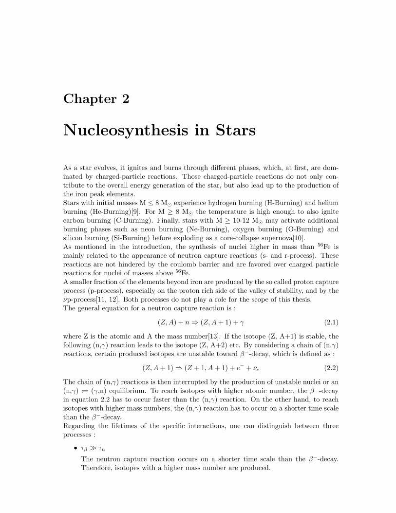
As a star evolves, it ignites and burns through different phases, which, at first, are dom-inated by charged-particle reactions. Those charged-particle reactions do not only con-tribute to the overall energy generation of the star, but also lead up to the production ofthe iron peak elements.Stars with initial masses M ≤ 8 M⊙ experience hydrogen burning (H-Burning) and heliumburning (He-Burning)[9]. For M ≥ 8 M⊙ the temperature is high enough to also ignitecarbon burning (C-Burning). Finally, stars with M ≥ 10-12 M⊙ may activate additionalburning phases such as neon burning (Ne-Burning), oxygen burning (O-Burning) andsilicon burning (Si-Burning) before exploding as a core-collapse supernova[10].As mentioned in the introduction, the synthesis of nuclei higher in mass than 56Fe ismainly related to the appearance of neutron capture reactions (s- and r-process). Thesereactions are not hindered by the coulomb barrier and are favored over charged particlereactions for nuclei of masses above 56Fe.A smaller fraction of the elements beyond iron are produced by the so called proton captureprocess (p-process), especially on the proton rich side of the valley of stability, and by theνp-process[11, 12]. Both processes do not play a role for the scope of this thesis.The general equation for a neutron capture reaction is :
(Z,A) + n ⇒ (Z,A+ 1) + γ (2.1)
where Z is the atomic and A the mass number[13]. If the isotope (Z, A+1) is stable, thefollowing (n,γ) reaction leads to the isotope (Z, A+2) etc. By considering a chain of (n,γ)reactions, certain produced isotopes are unstable toward β−-decay, which is defined as :
(Z,A+ 1) ⇒ (Z + 1, A+ 1) + e− + νe (2.2)
The chain of (n,γ) reactions is then interrupted by the production of unstable nuclei or an(n,γ) (γ,n) equilibrium. To reach isotopes with higher atomic number, the β−-decayin equation 2.2 has to occur faster than the (n,γ) reaction. On the other hand, to reachisotopes with higher mass numbers, the (n,γ) reaction has to occur on a shorter time scalethan the β−-decay.Regarding the lifetimes of the specific interactions, one can distinguish between threeprocesses :
• τβ ≫ τn
The neutron capture reaction occurs on a shorter time scale than the β−-decay.Therefore, isotopes with a higher mass number are produced.
4 Nucleosynthesis in Stars
• τn ∼ τβ
Both processes occur at a similar rate. This situation is encountered at so-calledbranching points.
• τβ ≪ τn
Here the β−-decay occurs on a shorter time scale than the neutron capture. Conse-quently isobars with higher atomic numbers are produced.
In general, the first case is typical for the classical r-process while the third case is charac-teristic for the s-process. The processes are distinguished by the required neutron densitywhich the nuclei need to be exposed to.The extreme conditions for the r-process are matched in explosive stellar environments,while the s-process is operating during hydrostatic burning phases of a star. Both processesfollow their own path on the chart of nuclides. One can find isotopes that are for exampleproduced only by the s-process and are called s-only isotopes, while there are also r-onlyand s-r-isotopes (of mixed origin).The scope of this thesis does not allow a detailed review of the r-process, while the s-process is the major process sensitive to the neutron releasing reactions 25Mg(α,n)28Si,26Mg(α,n)29Si and 18O(α,n)21Ne.
2.1 The Classical S-Process 5
2.1 The Classical S-Process
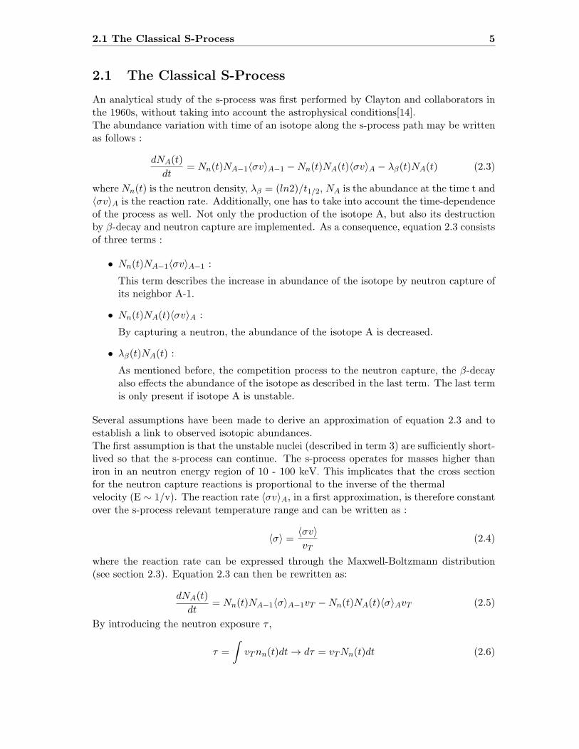
An analytical study of the s-process was first performed by Clayton and collaborators inthe 1960s, without taking into account the astrophysical conditions[14].The abundance variation with time of an isotope along the s-process path may be writtenas follows :
dNA(t)
dt= Nn(t)NA−1⟨σv⟩A−1 −Nn(t)NA(t)⟨σv⟩A − λβ(t)NA(t) (2.3)
where Nn(t) is the neutron density, λβ = (ln2)/t1/2, NA is the abundance at the time t and⟨σv⟩A is the reaction rate. Additionally, one has to take into account the time-dependenceof the process as well. Not only the production of the isotope A, but also its destructionby β-decay and neutron capture are implemented. As a consequence, equation 2.3 consistsof three terms :
• Nn(t)NA−1⟨σv⟩A−1 :
This term describes the increase in abundance of the isotope by neutron capture ofits neighbor A-1.
• Nn(t)NA(t)⟨σv⟩A :
By capturing a neutron, the abundance of the isotope A is decreased.
• λβ(t)NA(t) :
As mentioned before, the competition process to the neutron capture, the β-decayalso effects the abundance of the isotope as described in the last term. The last termis only present if isotope A is unstable.
Several assumptions have been made to derive an approximation of equation 2.3 and toestablish a link to observed isotopic abundances.The first assumption is that the unstable nuclei (described in term 3) are sufficiently short-lived so that the s-process can continue. The s-process operates for masses higher thaniron in an neutron energy region of 10 - 100 keV. This implicates that the cross sectionfor the neutron capture reactions is proportional to the inverse of the thermalvelocity (E ∼ 1/v). The reaction rate ⟨σv⟩A, in a first approximation, is therefore constantover the s-process relevant temperature range and can be written as :
⟨σ⟩ = ⟨σv⟩vT
(2.4)
where the reaction rate can be expressed through the Maxwell-Boltzmann distribution(see section 2.3). Equation 2.3 can then be rewritten as:
dNA(t)
dt= Nn(t)NA−1⟨σ⟩A−1vT −Nn(t)NA(t)⟨σ⟩AvT (2.5)
By introducing the neutron exposure τ ,
τ =
∫vTnn(t)dt → dτ = vTNn(t)dt (2.6)
6 Nucleosynthesis in Stars
equation 2.5 can be expressed as :
dNs(A)
dτ= σ(A− 1)Ns(A− 1)− σ(A)Ns(A) (2.7)
The change in abundance depends on the product σNs which varies smoothly with massnumber. Clayton introduced this approximation known as local approximation[13, 14].Seeger et al. were not able to reproduce the s-isotope abundances with one single neutronexposure[15]. The product of cross section and abundance is given by Seeger et al. inanalytical form by :
⟨σ⟩(A)Ns(A) =G ·N⊙
56
τ0
A∏i=56
(1 +1
τ0⟨σ⟩(i))−1 (2.8)
where N⊙56 is the observed solar 56Fe abundance and τ0, as well as G, are fit parameters.
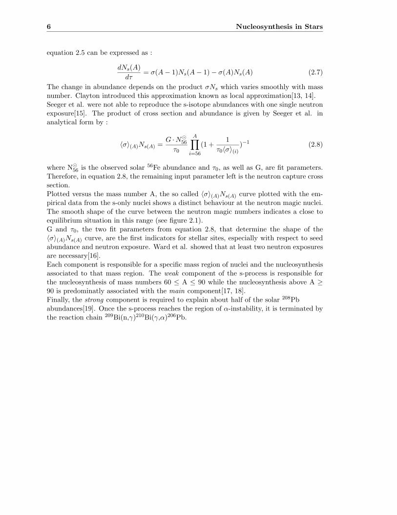
Therefore, in equation 2.8, the remaining input parameter left is the neutron capture crosssection.Plotted versus the mass number A, the so called ⟨σ⟩(A)Ns(A) curve plotted with the em-pirical data from the s-only nuclei shows a distinct behaviour at the neutron magic nuclei.The smooth shape of the curve between the neutron magic numbers indicates a close toequilibrium situation in this range (see figure 2.1).G and τ0, the two fit parameters from equation 2.8, that determine the shape of the⟨σ⟩(A)Ns(A) curve, are the first indicators for stellar sites, especially with respect to seedabundance and neutron exposure. Ward et al. showed that at least two neutron exposuresare necessary[16].Each component is responsible for a specific mass region of nuclei and the nucleosynthesisassociated to that mass region. The weak component of the s-process is responsible forthe nucleosynthesis of mass numbers 60 ≤ A ≤ 90 while the nucleosynthesis above A ≥90 is predominatly associated with the main component[17, 18].Finally, the strong component is required to explain about half of the solar 208Pbabundances[19]. Once the s-process reaches the region of α-instability, it is terminated bythe reaction chain 209Bi(n,γ)210Bi(γ,α)206Pb.
2.1 The Classical S-Process 7
Figure 2.1: The ⟨σ⟩(A)Ns(A) curve plotted versus the mass number A. The solid line iscalculated corresponding to the work of Seeger et al.[15].
2.1.1 S-Process Branchings
The competition between neutron captures and β−-decays is critical for determining thepath of the s-process. Therefore, the condition τβ ≪ τn represents the main characteristicfor the path of the s-process.
Nevertheless, some nuclei exhibit comparable neutron capture and β-decay rates (τn ∼ τβ),possibly resulting in a branching of the reaction flow. These nuclei are described as possiblebranching points of the s-process.
The occurence of a branching can be observed by comparing the abundance of nucleus(Z, A+1) with the abundance of nucleus (Z+1, A). Differences in the observed abundancescan lead to more detailed information about the physical environment, respectively theastrophysical site. For instance, s-process branching points can help determine the neutrondensity to which the seed nuclei had to be exposed to.
One can define the strength of a branching in terms of the β-decay rates λβ of the involvednuclei :
fβ =λβ
λβ + λn(2.9)
One can then calculate the neutron density nn analytically via:
nn =1− fβfβ
· 1
vT ⟨σ⟩i· ln(2)
t∗1/2(i)(2.10)
where i denotes the isotope at which the branching occurs.
As λβ is dependent on the temperature, each branching point can be used to deriveimportant information about the stellar environment. For different branching points,
8 Nucleosynthesis in Stars
different sets of parameters can be found, which constraint the astrophysical scenarios,that have to be taken into account[20].The canonical approach has been successful in describing not only the s-process branch-ing, but also the s-abundance distribution. However, as more (n,γ) cross sections wereexperimentally determined, the limitations of the canonical approach became evident.The isotope 142Nd is an s-process isotope and located at a drop of the ⟨σ⟩(A)Ns(A) curve.This drop is caused by the appearance of the neutron magic number N= 82 and thesubsequent low neutron capture cross section.
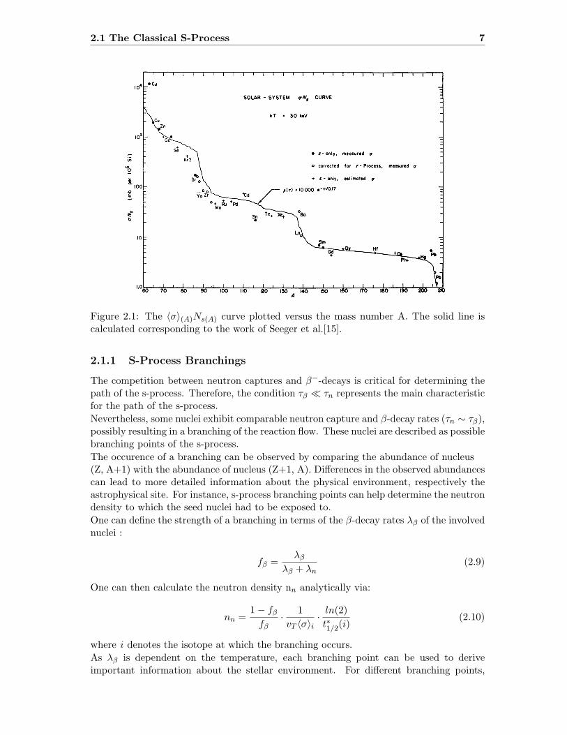
Figure 2.2: Illustrated is the s-process path in the mass region A=147-149. The isotopes148Sm and 150Sm are shielded from the r-process and determine the branching strength[20].A significant branching at A = 147 - 149 results in a higher ⟨σ⟩(A)Ns(A) value for 150Smcompared to 148Sm.
Wisshak et al. used their experimentally determined (n,γ) cross sections of the Nd isotopesto calculate the abundances of the Nd isotopes with the classical approach. Their resultsshowed a clear overproduction of the isotope 142Nd. The mismatch between the classicalapproach and observed abundances led to the conclusion that the classical approach isnot accurate enough to describe the stellar scenario in which the s-process takes place[21].Only nucleosynthesis calculations in realistic stellar models are able to reproduce in detailthe production of the s-process elements.

2.2 Stellar Sites for the S-Process 9
2.2 Stellar Sites for the S-Process
The neutrons for the (n,γ)-reactions are supplied by (α,n) reactions on specific nuclei[3, 4].These (α,n) reactions are known as stellar neutron sources. The primary stellar neutronsources are the reactions 13C(α,n)16O and 22Ne(α,n)25Mg. These reactions can take placeduring burning phases of the star in which helium is available.
Each component of the s-process needs to be assigned to different types of stars or theirrespective phases. This is mainly due to the different physical conditions needed to repro-duce the abundance patterns observed.
Low mass asymptotic giant branch (AGB) stars (M ≤ 8 M⊙) were determined to be thesites for the main and strong component[18, 22]. The weak component of the s-process isassigned to massive stars (M > 10 M⊙)[23].
2.2.1 AGB Stars
A star reaches the AGB phase after helium burning has been exhausted in the core. Atthis point the He-Burning continues in a shell, together with a more external hydrogenburning shell.
During most of the AGB phase, the energy to sustain the stellar structure is supplied bythe hydrogen shell. The temperature in the helium shell is not high enough to activatee.g. the triple-α process.
However, as the hydrogen shell processes more material, the temperature increases abovethe helium shell until helium burning is activated in a flash (Thermal Pulse, TP). This ismainly due to the high temperature dependence of the triple-α process.
The large energy generation during the TP induces a convective instability in the regionbetween the helium shell and the hydrogen shell (He-intershell region). The He-intershellregion expands by cooling and eventually reduces the hydrogen burning efficiency. TheTP typically lasts few hundred years until the triple-α process loses efficiency, again.
The He-intershell contracts and becomes radiative again, while the H-shell returns tohydrostatic burning[9].
After the TP, the hydrogen shell may eventually be deactivated and the convective envelopemay dredge up part of the He-intershell material. This causes mixing of fresh hydrogenbelow the previous hydrogen shell location (Third Dredge Up, TDU)[24].
The freshly supplied protons may be captured by 12C producing 13C through the12C(p,γ)13N(e+ ν)13C reaction chain. This process is located in a small radiative regionjust below the hydrogen shell known as 13C-pocket.
Within the 13C-pocket, the reaction 13C(α,n)16O burns at T9 ∼ 0.1 during the intershellphase, forming the s-process elements. The s-process enriched pocket is mixed into the He-intershell during the next TP. Following the TDU, the s-process elements may be dredgedup into the envelope. The neutron exposure produced within the 13C-pocket accountsfor about 95 % of the produced s-processe nuclides whereas the partial activation of thereaction 22Ne(α,n)25Mg during the TP accounts for the remaining 5%[22].
In terms of processed material and its isotopic composition, it is important to note that themetallicity of the star and the profile of the 13C-pocket remain as the crucial parameters.As Arlandini et al. were able to illustrate (see figure 2.3), AGB star models with solar-likemetallicity provide the best agreement with the main component of the s-process[18].

10 Nucleosynthesis in Stars
Figure 2.3: S-process abundance distribution that reproduces the solar system main s-component, with updated Nd cross sections. Obtained from Arlandini et al.[18].
2.2.2 Massive Stars
Massive stars, M ≥ 10 M⊙, are responsible for the production of the weak s-processcomponent[25].
During hydrogen burning 14N is being synthesized from the initial CNO isotopes andrepresents approximately 2 % of the core composition.14N will be converted into 22Ne via the reaction chain 14N(α,γ)18F(β+)18O(α,γ)22Ne. Atthe end of the helium core burning phase, the temperature is high enough (T9 ∼ 0.3)to efficiently activate 22Ne(α,n)25Mg. The reaction 22Ne(α,n)25Mg is the main neutronsource for the s-process in massive stars.
As convective core helium burning proceeds, the isotopes 12C, 16O, 20,22Ne and 25,26Mgbecome the most abundant. Carbon burning ignites in the core and in a convective shellat T9 ∼ 1. The energy release is mainly governed by the reactions :
12C +12 C → 24Mg∗ → 20Ne+ 4He (2.11)
→ 24Mg∗ → 23Na+ p (2.12)
→ 24Mg∗ → 23Mg + n (2.13)
With the release of α particles through the 12C(12C,α)20Ne reaction, α capture reactionsare activated and proceed over the ashes of the previous helium core. The strongest αcapture reactions are 16O(α,γ)20Ne, 20Ne(α,γ)24Mg and 22Ne(α,n)25Mg. With the carbonburning shell exhausting its 12C, the isotopes 16O, 20Ne, 23Na and 24Mg become the mostabundant leading up to the next burning stage. At the end of carbon burning, at solarmetallicities, 50% of 22Ne still remains[7].
The next burning stage, Neon burning (T9 ≃ 1.5), ignites after the central carbon exhaus-tion and is dominated by the reactions 20Ne(γ,α)16O and 20Ne(α,γ)24Mg.
At this point, strong neutron densities (∼ 1015 cm−3) are produced by the reactions25Mg(α,n)28Si and 26Mg(α,n)29Si[6, 26].

2.2 Stellar Sites for the S-Process 11
Figure 2.4: Energy generation of the advanced burning stages of a massive star relativeto the burning temperature. The dark line labeled ”Neutrinos” represents the neutrinolosses as a function of temperature[10].
Further burning stages such as oxygen burning are ignited subsequently until the life ofthe star ends with the iron core collapse and the following supernova explosion[10].As previously noted, the reaction 22Ne(α,n)25Mg is the main neutron source in massivestars. Most of the neutrons released from the reaction 22Ne(α,n)25Mg are captured by lightnuclei, described as neutron poisons. While the main part of the neutrons is captured inthe helium core and the carbon shell, a smaller fraction (∼ 20%) may be captured by Feseeds[23].Particulary the recycling effect plays an important role, in which the released neutronsare captured by light poisons but then later on are re-released. The main recycling pointinvolves the reaction cycles : 12C(n,γ)13C(α,n)16O and 16O(n,γ)17O(α,n)20Ne[7].For example, the competition of the reaction channels 18O(α,n)21Ne and 18O(α,γ)22Neplays a crucial role in determining the abundance of the Ne isotopes and the previouslymentioned neutron source 22Ne(α,n)25Mg.Any uncertainties in the determination of these competing reactions would result in aninaccurate description of the resulting neutron fluxes and isotopic abundances.

12 Nucleosynthesis in Stars
2.3 Nuclear Physics behind Nucleosynthesis
To be able to judge the amount of nuclear material synthesized within a certain time spane.g. a burning phase (see equation 2.3), one needs to determine the reaction rates of thereactions involved. The reaction rates are heavily dependent on the probability that thereactions occur, i.e., the cross section σ.By envisioning a projectile impinging on a target nucleus, one can describe σ, as theprobability to cause a well-defined reaction resulting in the release of reaction productsand energy. Moving from the classical to the quantum mechanical description of the nuclei,one has to take into consideration such properties as nuclear charge, angular momentum,projectile energy etc.The cross sections of interest are in general energy, and therefore velocity, dependent.Since the nuclear reactions of interest take place within stellar environments, it is helpfulto define the reaction rate of a specified reaction as the product of the incoming particleflux J = Nxv and effective reaction area F=σ(v)Ny :
r = NxNyvσ(v) (2.14)
where Nx (and Ny) define the number of particles per cubic centimeter. To characterizethe movement of the particles within the stellar gas, the product σv can be folded withthe velocity distribution
∫∞0 ϕ(v)dv = 1 :
⟨σv⟩ =∫ ∞
0ϕ(v)σ(v)vdv (2.15)
which then allows to define the total reaction rate as :
r = NxNy⟨σv⟩ (2.16)
The stellar gas can be considered as in thermodynamic equilibrium following the stabilitycriteria and energy conservation for a star. Therefore, the velocity distribution of theparticles can be described by a Maxwell-Boltzmann distribution. As the reaction rateincludes both interacting particles, it can be rewritten with the velocity distributions forboth particles :
⟨σv⟩ =∫ ∞
0
∫ ∞
0ϕ(vx)ϕ(vy)σ(v)vdvxdvy (2.17)
Rewriting vx and vy in terms of the relative velocity and the center of mass velocity V,one needs to use the total mass M and the reduced mass µ to describe the reaction rate :
⟨σv⟩ =(
8
πµ
)1/2 1
(kT )3/2
∫ ∞
0σ(E)Ee−
EkT dE (2.18)
Equation 2.18 shows, that the reaction rate is dependent not only on the cross section ofthe considered reaction but also on the stellar temperature. Therefore, the reaction ratehas to be calculated for ranges of temperatures, since the temperature changes as the starevolves[27].
2.3 Nuclear Physics behind Nucleosynthesis 13
2.3.1 The Astrophysical S-Factor
The investigation of (α,n) reactions requires the consideration of charged particle reactionsfirst. As a positively charged α-particle is moving towards the target nucleus, it will needto overcome the repulsive force known as the Columb barrier or penetrate it. Gamow wasable to show that a particle with an energy lower than the the Coulomb barrier, would beable to tunnel through the potential[28]. The particle then interacts with the nucleus andcauses a nuclear reaction. This process is occuring with a given probability P :
P =|Ψ(Rn)|2
|Ψ(Rc)|2(2.19)
where Rn represents the nuclear radius, Rc the classical turning point due to the Coulombbarrier and Ψ the wave function. For Rc ≫ Rn one can estimate the probability, alsoknown as the Gamow factor :
P = exp(−2πη) (2.20)
where η is the Sommerfeld parameter :
η =Z1Z2e
2
~v(2.21)
The cross section of charged particle reactions is not only dependent on the de Brogliewavelength :
σ ∝ πλ ∝ 1
E(2.22)
but also heavily dependent on the height of the Coulomb barrier :
σ ∝ exp(−2πη) (2.23)
The astrophysical S-factor S(E) is defined as :
σ =1
Eexp(−2πη)S(E) (2.24)
which varies smoothly for non-resonant reactions and is considered as one of the maincharacteristic quantities in Nuclear Astrophysics.Using equation 2.24, one can rewrite the reaction rate in equation 2.18 :
⟨σv⟩ =(
8
πµ
)1/2 1
(kT )3/2
∫ ∞
0S(E)exp
[− E
kT− b
E1/2
]dE (2.25)
with the barrier penetrability b given by :
b = (2µ)1/2πe2Z1Z2/~ (2.26)
For non-resonant reactions equation 2.25 is dominated by the behaviour of the exponentialterm. By multiplying both terms of the exponential function in the integrand, one canshow that the integrand leads to a peak close to an energy E0, the so called effectiveburning energy. The peak is known as Gamow peak, while the energy window underneathis known as Gamow window. Considering that the S-factor is almost constant over smallenergy windows, one can extract the S-factor out of the integrand in equation 2.25 :
⟨σv⟩ =(
8
πµ
)1/2 1
(kT )3/2S(E0)
∫ ∞
0exp
[− E
kT− b
E1/2
]dE (2.27)
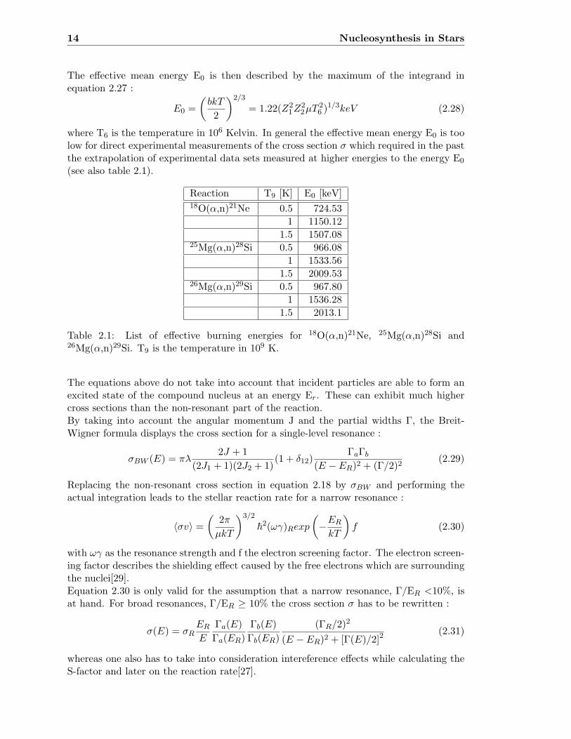
14 Nucleosynthesis in Stars
The effective mean energy E0 is then described by the maximum of the integrand inequation 2.27 :
E0 =
(bkT
2
)2/3
= 1.22(Z21Z
22µT
26 )
1/3keV (2.28)
where T6 is the temperature in 106 Kelvin. In general the effective mean energy E0 is toolow for direct experimental measurements of the cross section σ which required in the pastthe extrapolation of experimental data sets measured at higher energies to the energy E0
(see also table 2.1).
Reaction T9 [K] E0 [keV]18O(α,n)21Ne 0.5 724.53
1 1150.12
1.5 1507.0825Mg(α,n)28Si 0.5 966.08
1 1533.56
1.5 2009.5326Mg(α,n)29Si 0.5 967.80
1 1536.28
1.5 2013.1
Table 2.1: List of effective burning energies for 18O(α,n)21Ne, 25Mg(α,n)28Si and26Mg(α,n)29Si. T9 is the temperature in 109 K.
The equations above do not take into account that incident particles are able to form anexcited state of the compound nucleus at an energy Er. These can exhibit much highercross sections than the non-resonant part of the reaction.By taking into account the angular momentum J and the partial widths Γ, the Breit-Wigner formula displays the cross section for a single-level resonance :
σBW (E) = πλ2J + 1
(2J1 + 1)(2J2 + 1)(1 + δ12)
ΓaΓb
(E − ER)2 + (Γ/2)2(2.29)
Replacing the non-resonant cross section in equation 2.18 by σBW and performing theactual integration leads to the stellar reaction rate for a narrow resonance :
⟨σv⟩ =(
2π
µkT
)3/2
~2(ωγ)Rexp(−ER
kT
)f (2.30)
with ωγ as the resonance strength and f the electron screening factor. The electron screen-ing factor describes the shielding effect caused by the free electrons which are surroundingthe nuclei[29].Equation 2.30 is only valid for the assumption that a narrow resonance, Γ/ER <10%, isat hand. For broad resonances, Γ/ER ≥ 10% the cross section σ has to be rewritten :
σ(E) = σRER
E
Γa(E)
Γa(ER)
Γb(E)
Γb(ER)
(ΓR/2)2
(E −ER)2 + [Γ(E)/2]2(2.31)
whereas one also has to take into consideration intereference effects while calculating theS-factor and later on the reaction rate[27].
2.4 Reaction Networks 15
2.4 Reaction Networks
The use of nuclear reaction networks in stellar models allows to properly simulate thenucleosynthesis of isotopes. Precise experimental reaction rates are the key for accuratenucleosynthesis calculations. A reaction network is given by a list of isotopes properlylinked by a complete set of nuclear reaction rates (see section 2.1).The nucleus of the isotope i undergoes four different types of nuclear reactions :
• the destruction of the nucleus via a two-body reaction
• the production of the nucleus via a two-body reaction
• β−-decay where the nucleus is the daughter and therefore being produced
• β−-decay where the nucleus is the mother and therefore being destroyed
With Yi defined as the molar fraction of an isotope i, ρ the density and NA the Avogadronumber, one can establish a differential equation to describe the evolution over a certaintime t :
dYidt
= ρNA
−∑j
YiYj⟨σv⟩ij +∑l
YlYk⟨σv⟩lk − Yiλi + Ymλm
(2.32)
where each term respectively represents the above mentioned nucleosynthesis steps. Inequation 2.32 three body reactions, etc. are not included.In this work the NUGRID PPN post-processing code will be employed, which has beendeveloped by Herwig et al.[5, 30, 31]. The post-processing code relies on previous stellarmodel calculations for the basic structure of a stellar scenario. It allows to calculatecomplete isotopic abundances for different stages of the stellar evolution.Essential is the use of most accurate experimental data for the use of the reactions rates.The achieved results by these computational calculations can then be compared withobservational evidence and give indications about the accuracy of the stellar models andexperimental data sets used.
16 Nucleosynthesis in Stars
2.5 Observational Evidence - Meteoritic Grains
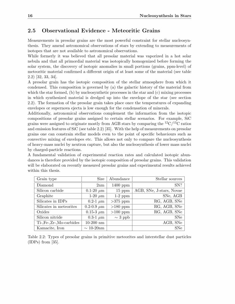
Measurements in presolar grains are the most powerful constraint for stellar nucleosyn-thesis. They amend astronomical observations of stars by extending to measurements ofisotopes that are not available to astronomical observations.While formerly it was believed that all presolar material was vaporized in a hot solarnebula and that all primordial material was isotopically homogenized before forming thesolar system, the discovery of isotopic anomalies in small portions (grains, ppm-level) ofmeteoritic material confirmed a different origin of at least some of the material (see table2.2) [32, 33, 34].A presolar grain has the isotopic composition of the stellar atmosphere from which itcondensed. This composition is governed by (a) the galactic history of the material fromwhich the star formed, (b) by nucleosynthetic processes in the star and (c) mixing processesin which synthesized material is dredged up into the envelope of the star (see section2.2). The formation of the presolar grain takes place once the temperatures of expandingenvelopes or supernova ejecta is low enough for the condensation of minerals.Additionally, astronomical observations complement the information from the isotopiccompositions of presolar grains assigned to certain stellar scenarios. For example, SiCgrains were assigned to originate mostly from AGB stars by comparing the 12C/13C ratiosand emission features of SiC (see table 2.2) [35]. With the help of measurements on presolargrains one can constrain stellar models even to the point of specific behaviours such asconvective mixing of envelopes etc. This allows not only to compare the nucleosynthesisof heavy-mass nuclei by neutron capture, but also the nucleosynthesis of lower mass nucleiby charged-particle reactions.A fundamental validation of experimental reaction rates and calculated isotopic abun-dances is therefore provided by the isotopic composition of presolar grains. This validationwill be elaborated on recently measured presolar grains and experimental results achievedwithin this thesis.
Grain type Size Abundance Stellar sources
Diamond 2nm 1400 ppm SN?
Silicon carbide 0.1-20 µm 15 ppm AGB, SNe, J-stars, Novae
Graphite 1-20 µm 1-2 ppm SNe, AGB
Silicates in IDPs 0.2-1 µm >375 ppm RG, AGB, SNe
Silicates in meteorites 0.2-0.9 µm >180 ppm RG, AGB, SNe
Oxides 0.15-3 µm >100 ppm RG, AGB, SNe
Silicon nitride 0.3-1 µm ∼ 3 ppb SNe
Ti-,Fe-,Zr-,Mo-carbides 10-200 nm AGB, SNe
Kamacite, Iron ∼ 10-20nm SNe
Table 2.2: Types of presolar grains in primitive meteorites and interstellar dust particles(IDPs) from [35].
Chapter 3
Previous Results
As mentioned previously (see section 2.2.2), the reactions 25Mg(α,n)28Si and 26Mg(α,n)29Sibecome neutron sources during the neon burning phase in massive stars. Additionally,the competition between the reactions 18O(α,n)21Ne and 18O(α,γ)22Ne is crucial for therecycling effect and the synthesis of the neon isotopes. The ideal situation would be tohave reliable experimental data at stellar temperatures to accurately judge the impact ofthose reactions.Calculating the effective mean energy for these reactions following equation 2.28 at dif-ferent temperatures (see also table 2.1), leads to the conclusion that the reactions haveto be measured accurately below a laboratory energy of 1500 keV. In this chapter it willbe shown that sufficient experimental data in this energy range has not been available todate.
18 Previous Results
3.1 25Mg(α,n)28Si & 26Mg(α,n)29Si
In 1962, Bair et al. were the first to report successful measurements on 26Mg(α,n)29Si[36].Unfortunately, their measurements were only performed down to a laboratory energy of3.1 MeV which is not sufficient for nucleosynthesis purposes. Their measurements havean error of up to 50%, due to the unknown contaminations of their targets. They wereespecially concerned with the ratio between MgO and Mg in their targets, since theyevaporated MgO onto a tantalum backing and were not able to determine the Mg:MgOratio and the target thickness.
Russell et al. used a similiar technique as Bair et al. and extended the energy rangefor their measurements down to 2.5 MeV[37]. For the detection of the promptly releasedneutrons a BF3 counter was used, which did not allow a direct separation of neutrons-from the reaction 26Mg(α,n)29Si or neutrons being released from other reactions such as13C(α,n)16O. The quality of spectroscopic information from γ-spectra was further dimin-ished by the occurence of the 13C(α,n)16O reaction as well an the use of NaI(Tl) detectors.Russell and his colleagues used evaporated targets in which MgO was mixed with zirco-nium. It was believed that zirconium reduced MgO and that the resulting elementalmagnesium evaporated onto copper backings. No information on the possible oxygen,respectively MgO, content of the targets is given.
Namjoshi and Bassey II were the only ones later performing experiments to lower energiesafter Russell, but not down to energies essential for Nuclear Astrophysics[38, 39]. On theother hand, there seemed to be no strong need to investigate the reactions 25Mg(α,n)28Siand 26Mg(α,n)29Si, since 13C(α,n)16O and 22Ne(α,n)25Mg were considered as the majorneutron sources for different burning phases in stellar scenarios.
Van de Zwan and colleagues were the first ones to report the cross sections for 25Mg(α,n)28Sidown to a laboratory energy of 1.8 MeV using similar techniques as Bair et al.[40].
These authors used different backing materials, but did not mention any contamination oftheir targets by carbon or oxygen. In addition the use of surface barrier detectors provedto be unsuitable for neutron spectroscopy.
Motivated by the work of Howard et al., Anderson and his colleagues were able to measureboth reactions down to an energy of 1.6 MeV and to determine the respective reactionrates[41, 42]. Their goal was to determine whether both reactions could play a role asneutron sources during explosive neon buring at temperatures T9 ∼ 3. As detectiontechniques two methods were employed : The first one was a germanium detector to detectthe γ-rays, while a long counter based on BF3 tubes was used to detect the neutrons.This allowed for the correction of additional neutrons being released by the prominentbackground reactions 13C(α,n)16O and 18O(α,n)21Ne. Evaporated targets were used whereMgO was reduced with tantalum powder and then evaporated onto tantalum backings.The thickness of the targets was determined via resonances of the reactions 25Mg(p,γ)26Aland 26Mg(p,γ)27Al.
No information about the physical location of the background reactions is given. A possiblecontamination of the beamline or the target itself is not taken into consideration. Secondly,energy steps of 50 keV were performed which does not allow the resolution of possiblenarrow resonances. The use of detection systems with an over all efficiency of a few percentand a reported failure in the detection system contributed further to the uncertainties.Anderson and his colleagues did not compare their experimental results with those ofprevious authors. They conclude that the reactions 25Mg(α,n)28Si and 26Mg(α,n)29Sicould possibly play a role during the process proposed by Howard et al.
3.1 25Mg(α,n)28Si & 26Mg(α,n)29Si 19
Kuchler & Wieland Measurements
Kuchler investigated both reactions utilizing spectroscopy of the released neutrons. Forhis measurements he used liquid scintillators (Type NE213) at 0, 60 and 90 degrees inorder to be able to gain spectroscopic information[43]. Additionally, a 3He ionizationchamber was used for a few measurements. Evaporated Mg targets were used whichwere produced via the reduction of MgO and the following evaporation onto oxygen-free (OFHC) copper. Similar to previous authors no precise measurements of the actualtarget thickness were performed. No information on the contamination of the targetsregarding carbon and oxygen is reported. Since the targets were produced at the MPIfur Kernphysik in Heidelberg and then transported to Stuttgart, possible oxidation of theMg-layer should have been taken into account. In fact, Kuchler was able to show thatlayers of oxygen contributed to his experimental data by comparing them to measurementspreviously performed by Bair et al.[44]. He also notes that even the use of spectroscopicdetectors did not allow the separation of neutrons being released for example by the17O(α,n)20Ne reaction from those released by the magnesium reactions. Additionally, theauthor does not report in detail how possible background contributions were subtractedfrom the experimental data. Additional problems are indicated by the observation thatthe used targets showed burn and blistering effects after irradiation. The target thicknessmust have been reduced over time and, if not checked on a regular base, the experimentaldata were not accurately analyzed.
In spite of this, Kuchler calculated the S-factor for both reactions. For 26Mg(α,n)29Si theS-factor was rising for lower energies and for 25Mg(α,n)28Si the S-factor was a smoothfunction. No information is given on reaction rates and possible influence on stellar nu-cleosynthesis.
Wieland reanalyzed the experimental data given by Kuchler. He came to the conclusion,that the 13C impurities and the according corrections concerning the 13C(α,n)16O reactionwere not performed correctly. Implementing a new analysis method and not being able todraw the same conclusion led to the need of new measurements[45].
For these, a neutron detector based on 16 3He tubes embedded in a 4π polyethylene matrixwas used. Another improvement was the use of implanted targets to reduce the impuritiesand therefore the background. The beamline setup was improved to reduce beam inducedbackground reactions.
The use of a 4π neutron detector with high efficiency resulted in an improvement inyields and therefore reduced beamtime and target destruction. However, no detailedinformation on the detection efficiency and its determination is given. Wieland only refersto the Monte-Carlo code MCNP and the determination of the efficiency only based oncomputational calculations. In general, spectroscopy would be only possible if one is ableto separate the counting rates in the different 3He tubes and assign them to differentneutron energies. This was not possible with the neutron detector available to Wieland.
An area of concern is the lack of information about the used targets. Wieland only notesthe implantation parameters of his implanted targets but did not determine the targetthickness experimentally. He also used targets previously used by Kuchler, but did notdiscuss possible oxidation of those targets as well.
The usage of gold-plated Cu backings showed improvements in the overall backgroundcontribution but remains as a concern. Especially the reported observation of 13C(α,n)16Oresonances leads to the conclusion, that the background contribution was still too high foraccurate magnesium target measurements.
20 Previous Results
(keV)aE
1000 1500 2000 2500 3000
(ba
rn)
s
-810
-710
-610
-510
-410
-310
-210
-110
van de Zwan, 1981
Anderson, 1983
Wieland, 1995
chler, 1990uK
HFB
Si 28,n)aMg(25
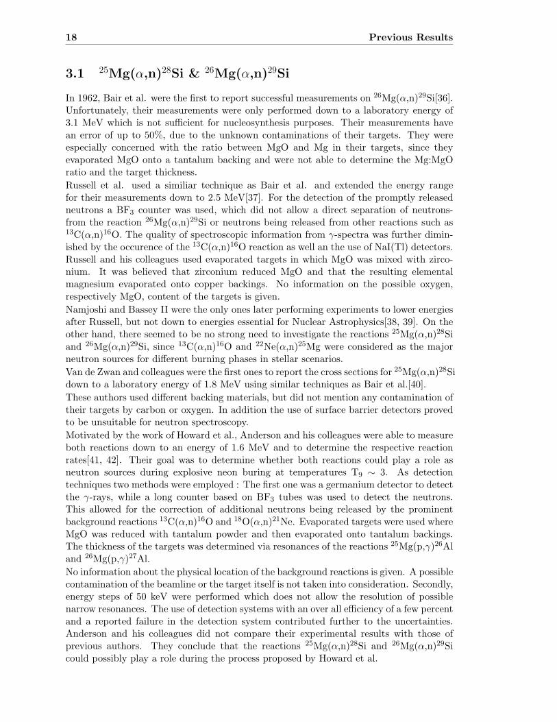
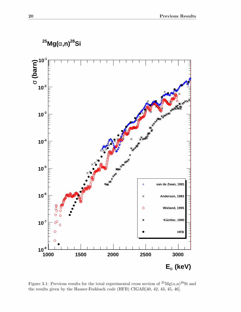
Figure 3.1: Previous results for the total experimental cross section of 25Mg(α,n)28Si andthe results given by the Hauser-Feshbach code (HFB) CIGAR[40, 42, 43, 45, 46].

3.1 25Mg(α,n)28Si & 26Mg(α,n)29Si 21
(keV)aE
1000 1500 2000 2500 3000
(ba
rn)
s
-810
-710
-610
-510
-410
-310
-210
-110
chler, 1990uK
Anderson, 1983
Wieland, 1995
HFB
Si29,n)aMg(26
Figure 3.2: Previous results for the total experimental cross section of 26Mg(α,n)29Si andthe results given by the Hauser-Feshbach code (HFB) CIGAR[42, 43, 45, 46].

22 Previous Results
Additionally, the possible contribution of 17O(α,n)20Ne and 18O(α,n)21Ne due to oxida-tion is not considered. Probably the lack of accurate experimental data gave no solidfoundation for possible arguments toward background contributions by 17O(α,n)20Ne and18O(α,n)21Ne. With these constraints on his experimental data, Wieland only derivedupper limits for the cross section of 25Mg(α,n)28Si and 26Mg(α,n)29Si below 1.5 MeV.Wieland also investigated the behaviour of the S-factor and the reaction rate of bothreactions, comparing them to the theoretical data given by Woosley and Caughlan [47, 48].For a temperature range of T9 = 0.1 - 10 the reaction rates differed up to a factor of 5,especially in the low temperature region. Wieland concludes in his diploma thesis that thereactions 25Mg(α,n)28Si and 26Mg(α,n)29Si have an impact on nucleosynthesis but doesnot give quantitative arguments.
3.1 25Mg(α,n)28Si & 26Mg(α,n)29Si 23
(keV)cmE1000 1200 1400 1600 1800 2000 2200 2400 2600
S-F
acto
r (M
eV b
)
910
1010
1110
1210
van de Zwan, 1981
Anderson, 1983
Wieland, 1995
Wieland, upper limits, 1995
Si 28,n)aMg(25
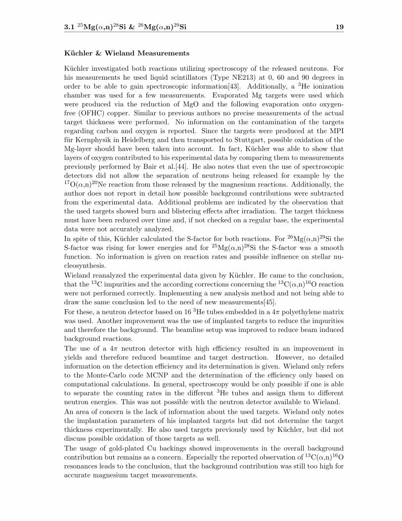
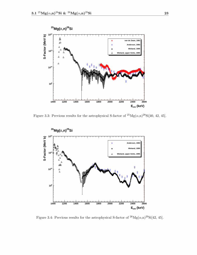
Figure 3.3: Previous results for the astrophysical S-factor of 25Mg(α,n)28Si[40, 42, 45].
(keV)cmE1000 1200 1400 1600 1800 2000 2200 2400 2600
S-F
acto
r (M
eV b
)
910
1010
1110
1210
Anderson, 1983
Wieland, 1995
Wieland, upper limits, 1995
Si 29,n)aMg(26
Figure 3.4: Previous results for the astrophysical S-factor of 26Mg(α,n)29Si[42, 45].
24 Previous Results
Current State of Research
Since the results of Kuchler and Wieland were obtained, new theoretical information on thepossible role of 25Mg(α,n)28Si and 26Mg(α,n)29Si has become available (e.g. [6, 7]). Theimprovement of stellar models and nucleosynthesis codes shows a need for more accurateexperimental data, as do measurements on presolar grains from meteorites, the results ofwhich indicate inconsistencies with the currrent reaction rates.
To explain anomalous isotopic abundances of the silicion isotopes in main-stream SiCgrains, Brown et al. proposed a scenario called magnesium burning[49]. The proposedastrophysical site for magnesium burning are AGB stars with M ∼ 6-9M⊙. By artificialadjustments of their model, Brown et al. were able to reproduce the abundance patternsof the Si isotopes found in mainstream SiC grains from AGB stars. In their conlusionsthey ask for experimental nuclear data to allow a detailed analysis of their model.
As pointed out by Hoppe et al., however, the proposed Mg burning process by Brown etal. and the implied astrophysical model did not agree with measurements on SiC grains[50]. Hoppe notes that the correlation of isotopic abundances of one isotopic chain doesnot allow to make accurate assumptions upon the astrophysical model. For example, asone adjusts the astrophysical model to reproduce the isotopic ratios of the Si isotopesby introducing 25Mg(α,n)28Si and 26Mg(α,n)29Si as possible sources, one has to take intoaccount higher neutron fluxes as well. These increased neutron fluxes immediately effectthe nucleosynthesis of isotopes sensitive to neutron capture nucleosynthesis. By takinginto account the abundances of 50Ti and not being able to reproduce them with Brown’smodel of the Mg burning process, Hoppe showed that such a process is not suitable forsingle AGB star models.
The conclusion drawn by Hoppe was followed by discussions about the stellar origin ofthe isotopic ratios of the Si isotopes which has been carrying on until today. As newcomputational codes and nuclear data became available, the stellar origin was assigned tomultiple AGB stars with different metallicities[51, 52, 53].
The discovery of an usual presolar SiC grain of type X (supernova origin) turned the at-tention of Hoppe and his colleagues on oxygen and neon burning zones based on the stellarmodels developed by Rauscher et al.[54, 55]. The isotopic abundance ratios predicted bythe stellar models were however not reproduced and led to a detailed investigation bythese authors. The reactions rates used by Rauscher and adopted by Hoppe et al. arebased on the calculations by Fowler et al. and the NACRE collaboration[56, 57].
The reaction rates for 25Mg(α,n)28Si and 26Mg(α,n)29Si of the NACRE collaboration arebased upon the experimental data of Wieland and therefore include the inconsistenciesregarding the S-factor and the reaction rates discussed above. This leads to reactions ratesthat are consistently higher than previously obtained values, also acknowledged by Hoppeand collaborators.
Network calculations of O/Si and O/Ne zones involving carbon as well as oxygen burningwere performed with modified reaction rates to estimate the possible influence on the Siisotopic abundance distribution. The conclusion of Hoppe et al. is, that the reaction rateof 26Mg(α,n)29Si should be increased by a factor of 2-3 (depending on the stellar model)in order to reproduce the observed abundance patterns.
Hoffman et al. independently carried out network calculations concerning nucleosynthe-sis in massive stars[6]. One result of their calculations is, that during convective car-bon and neon burning the reaction 26Mg(α,n)29Si could lead to the synthesis of nucleithat are usually bypassed by the s-process. Following Hoffman’s results, Pignatari was

3.1 25Mg(α,n)28Si & 26Mg(α,n)29Si 25
able to illustrate that during convective carbon burning the reactions 25Mg(α,n)28Si and26Mg(α,n)29Si should not play an important role (see figure 3.6) [7]. Their results rely onthe reaction rates achieved by Wieland as well.As it will be elaborated later, calculations based on the NUGRID PPN network code showsimilar effects, for example on the distribution of the Ba isotopes.Both, stellar models and measurements on presolar grains, therefore show a need for moreaccurate experimental data on the reactions 25Mg(α,n)28Si and 26Mg(α,n)29Si at energiesof astrophysical interest.
26 Previous Results
0
1
2
3
4
Ra
tio
/So
lar
0
1
2
3
4
44T
i/4
8Ti * 100
29Si/ 28Si 30Si/ 28Si 12C/13C 44Ti/ 48Ti
Grain KJB2-11-17-115 M SNII model
15 M SNII model,29Si yield enhanced
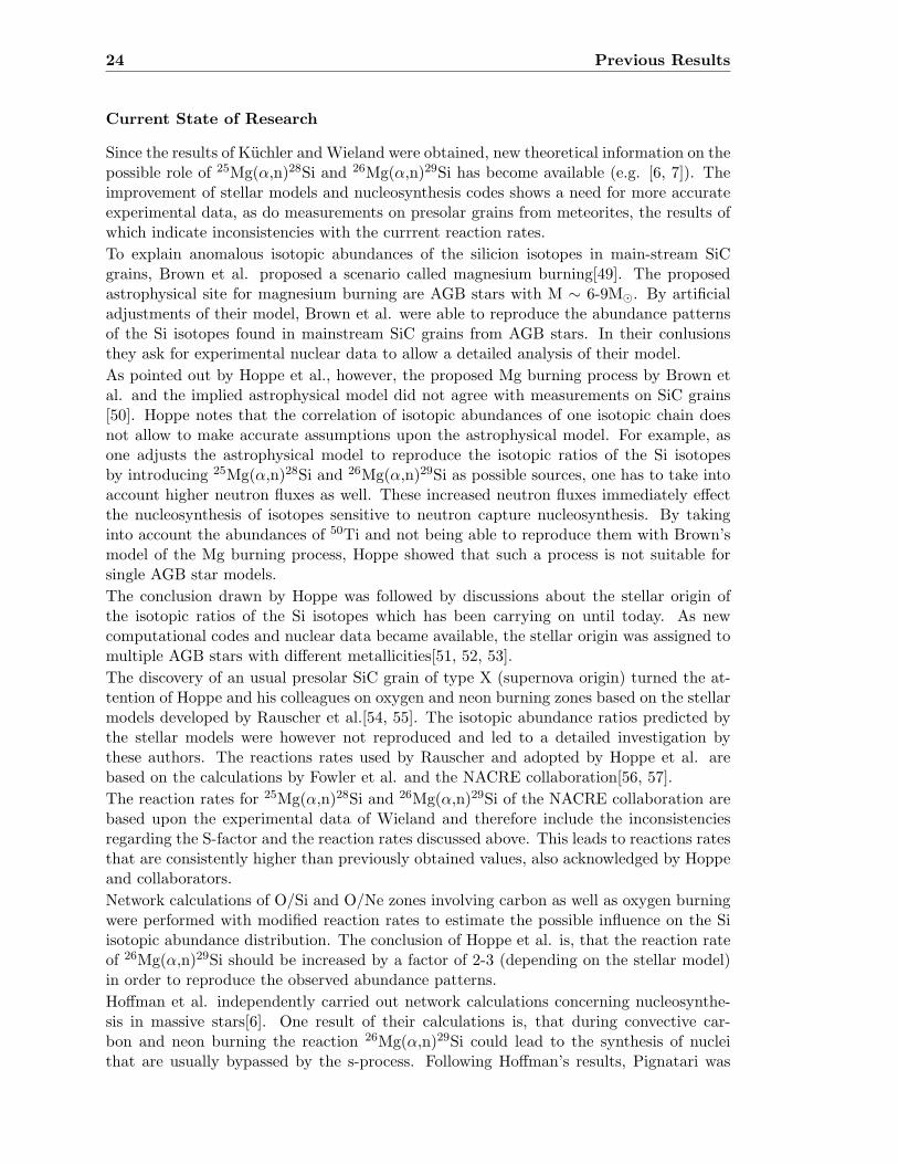
Figure 3.5: Shown are the isotopic ratios of a presolar grain found by Hoppe et al. com-pared to calculations performed with an enhanced reaction rate of 26Mg(α,n)29Si. Thematch of the calculations with an artificially enhanced reaction rate with the presolar grainmeasurements shows the need for an improved experimental data set of 26Mg(α,n)29Si[54].
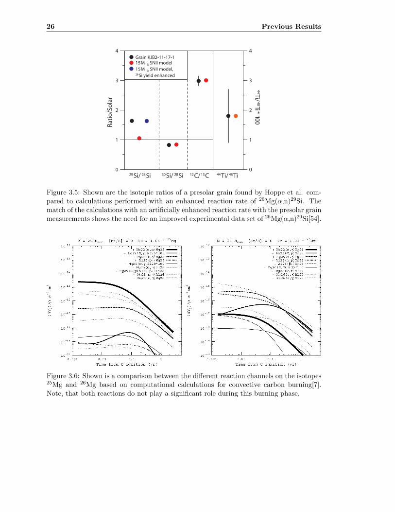
Figure 3.6: Shown is a comparison between the different reaction channels on the isotopes25Mg and 26Mg based on computational calculations for convective carbon burning[7].Note, that both reactions do not play a significant role during this burning phase.
3.2 18O(α,n)21Ne 27
3.2 18O(α,n)21Ne
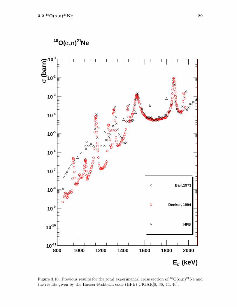
Bair et al. were the first ones to measure the reaction 18O(α,n)21Ne at energies relevant fornuclear astrophysics[36, 44]. They were able to determine the cross section to an laboratoryenergy of about 1050 keV. However, their improved experimental techniques (e. g. a gastarget system) did not allow an accurate analysis for the purpose of Nuclear Astrophysics.The data of Bair et al. suffered mainly from low resolution, low 18O enrichment and thebackground contribution from the reaction 13C(α,n)16O.Denker was able to determine the reaction rate of 18O(α,n)21Ne down to the thresholdenergy Ethres = 850.95 keV[8]. A sophisticated gas target system as well as a highlyenriched target gas were used to perform the experimental measurements. Denker was alsofirst in addressing the comparison of the reaction channels 18O(α,γ)22Ne and 18O(α,n)21Ne(section 2.2.2). Until today, the measurements by Denker have not been confirmed by anindependent experiment, however.More recent measurements of the reaction 18O(α,γ)22Ne revealed new details about itsreaction rate. Dababeneh et al. were able to evaluate the influence of their experimen-tal results on the reaction rate, but did not draw a comparison to the 18O(α,n)21Nereaction[58]. Similar to 25Mg(α,n)28Si and 26Mg(α,n)29Si, Pignatari was able to show,that 18O(α,n)21Ne does not play a role during carbon burning as well (see figure 3.7) [7].
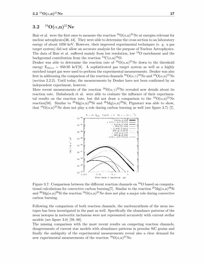
Figure 3.7: Comparison between the different reaction channels on 18O based on computa-tional calculations for convective carbon burning[7]. Similar to the reaction 25Mg(α,n)28Siand 26Mg(α,n)29Si the reaction 18O(α,n)21Ne does not play a major role during convectivecarbon burning.
Following the comparison of both reaction channels, the nucleosynthesis of the neon iso-topes has been investigated in the past as well. Specifically the abundance patterns of theneon isotopes in meteoritic inclusions were not represented accurately with current stellarmodels (see figure 3.8) [59, 60].The missing comparison with the most recent results on competing reaction channels,disagreements of current star models with abundance patterns in presolar SiC grains andfinally the ambiguity of the experimental measurements reveal also a clear demand fornew experimental measurements of the reaction 18O(α,n)21Ne.
28 Previous Results
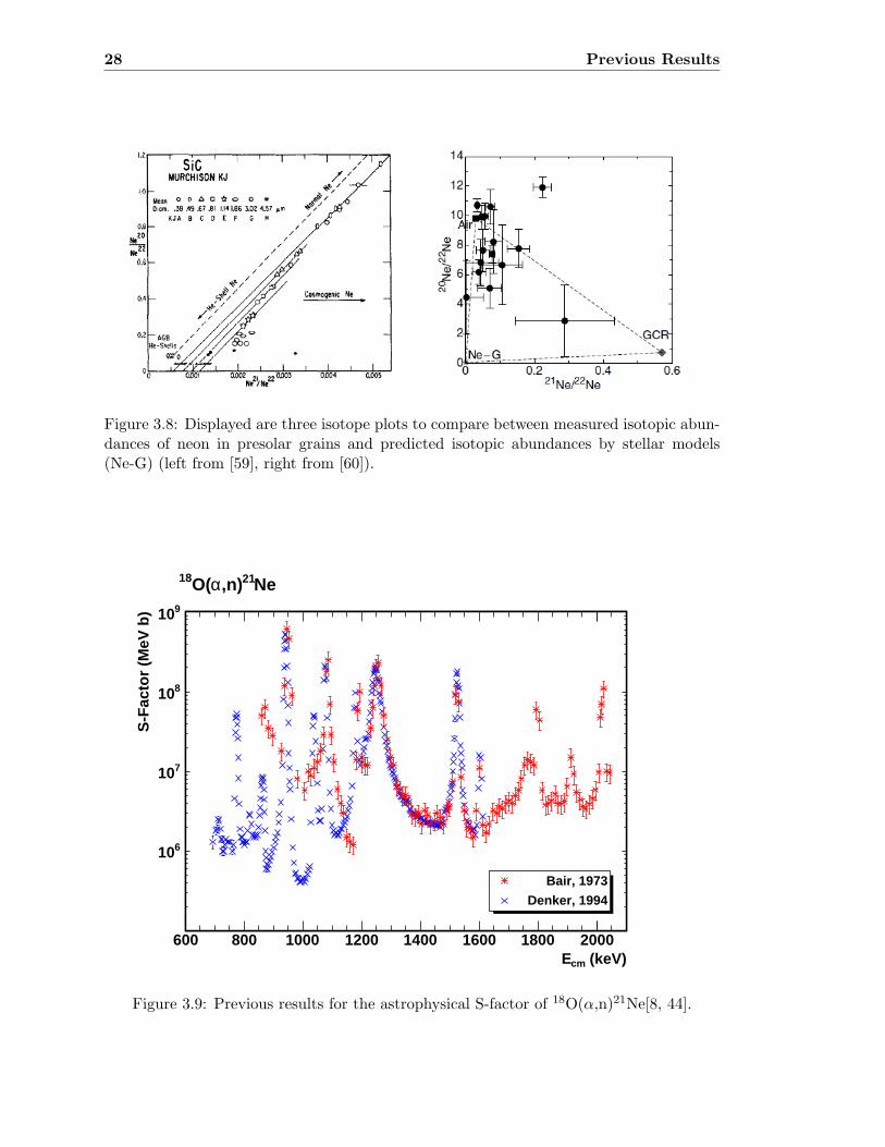
Figure 3.8: Displayed are three isotope plots to compare between measured isotopic abun-dances of neon in presolar grains and predicted isotopic abundances by stellar models(Ne-G) (left from [59], right from [60]).
(keV)cmE600 800 1000 1200 1400 1600 1800 2000
S-F
acto
r (M
eV b
)
610
710
810
910
Bair, 1973
Denker, 1994
Ne 21,n)aO(18
Figure 3.9: Previous results for the astrophysical S-factor of 18O(α,n)21Ne[8, 44].
3.2 18O(α,n)21Ne 29
(keV)aE
800 1000 1200 1400 1600 1800 2000
(ba
rn)
s
-1110
-1010
-910
-810
-710
-610
-510
-410
-310
-210
-110
Bair,1973
Denker, 1994
HFB
Ne21,n)aO(18
Figure 3.10: Previous results for the total experimental cross section of 18O(α,n)21Ne andthe results given by the Hauser-Feshbach code (HFB) CIGAR[8, 36, 44, 46].

30 Previous Results
Chapter 4
Experimental Techniques andProcedures
Nuclear reactions are verified by the detection of their reaction products. For the case of18O(α,n)21Ne, 25Mg(α,n)28Si and 26Mg(α,n)29Si, the reaction products are a neutron andan excited nucleus. The neutron emerges from the target while the excited nucleus decaysvia γ-decay into its ground state.After reviewing the different possible detector techniques, it was decided to detect theneutrons resulting from the reactions. The advantage detecting the neutrons comparedto the γ-rays is a high detection efficiency and a relatively flat efficiency behavior. Forthe acceleration of the α-particles, the KN Van-de-Graaff accelerator (KN) at the NuclearScience Laboratory at the University of Notre Dame (NSL) was used. The particle beamwas directed onto evaporated and anodized targets. Five experimental beam times wereperformed, during which accelerator calibration, detector calibration and production runswere executed.

32 Experimental Techniques and Procedures
4.1 The KN Accelerator and Beam Transport System
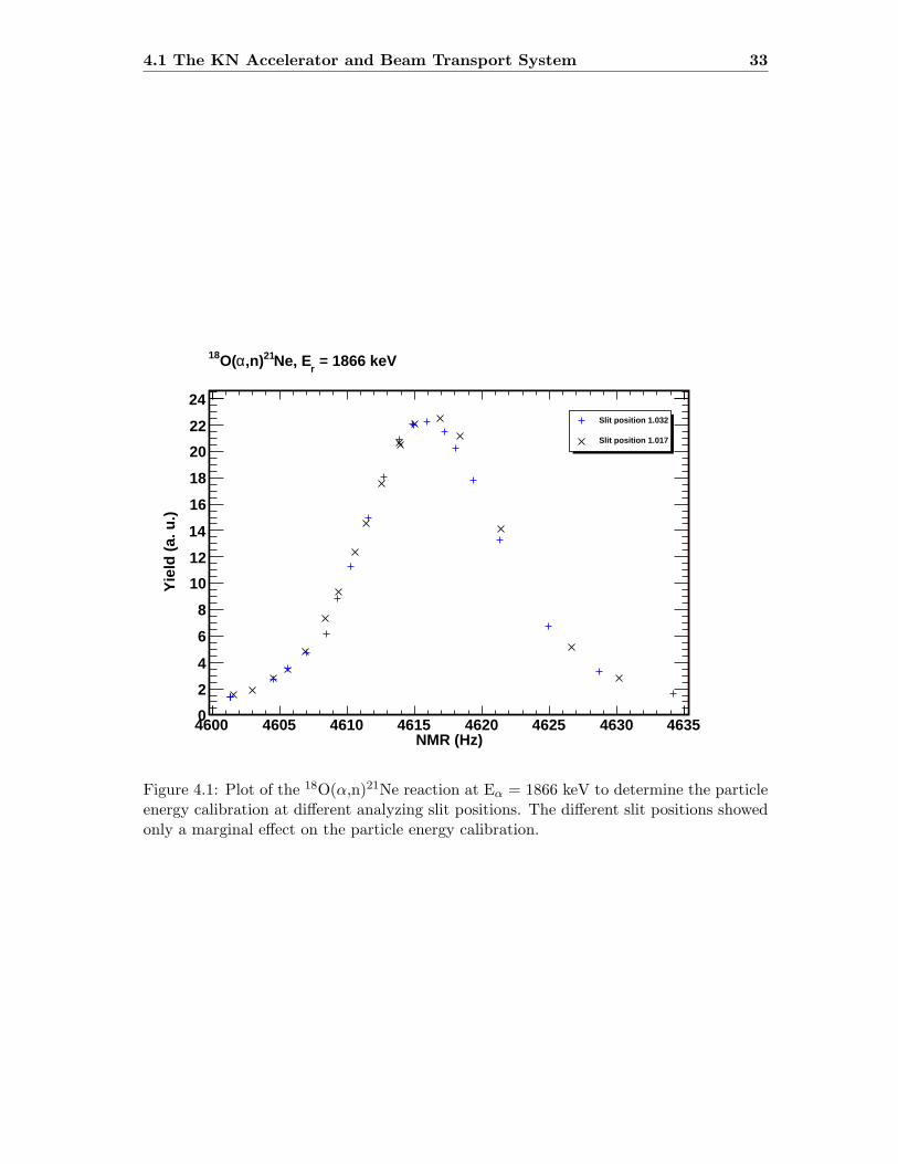
The experiments were exclusively performed at the NSL and the KN accelerator. The KNaccelerator is a single-ended Van-de-Graaff accelerator containing an internal RF-tubeion source. The ion source allows to switch between α-beam and proton-beam withoutopening the tank of the accelerator. The experiments were performed at energies between700 and 2700 keV.As the accelerated ions leave the accelerator tank, they enter a high-vacuum, ion opticalbeam transport system (beam line) which carries and directs the beam to the desiredtarget. The first ion optical element of importance is the analyzing magnet and its slits(analyzing slits) located behind the analyzing magnet. To ensure that the particles im-pinging on the target have the same energy, they are sent through the analyzing magnet.The field in the magnet is set, so that the particles having the desired energy are redi-rected while other particles do not pass the analyzing magnet. The analyzing slits ensure,that the terminal voltage of the accelerator is adjusted to the right particle energy. Themagnetic field is measured via a NMR probe.Before each experimental beam time, the magnetic field setting of the analyzing magnetwas calibrated with respect to particle energy. This was realized by changing the particleenergy until a known resonance of a specific reaction was observed. One can then correlatethe resonance energy with the field setting in the analyzing magnet and derive a calibra-tion function for the particle energy. A similar method is the measurement across thethreshold of a well known reaction. Both methods were used multiple times and involvedthe reactions 27Al(p,γ)28Si, 51V(p,n)51Cr and 18O(α,n)21Ne (see table 4.1 and figure 4.1)[27, 61, 62].
Reaction Elab [keV] Type of energy calibration Particle detected27Al(p,γ)28Si 992 Resonance γ18O(α,n)21Ne 1866 Resonance neutron51V(p,n)51Cr 1565 Threshold neutron
Table 4.1: List of reactions used for the KN energy calibration before every experimentalbeam time.
As the particle beam exits the analyzing magnet, a second magnet (switching magnet)directs the beam. The beam is directed either to a beamline designed for Rutherford-Backscattering (RBS beamline) measurements or to a beamline for measurements of (p,γ)and (α,n) reactions (0 beamline).
4.1.1 RBS Beamline
Rutherford-Backscattering is a technique that utilizes the scattering of incoming particleson a thin film probe (for example a target) to determine its composition.Based on the evaluations of previous measurements of the 25Mg(α,n)28Si and 26Mg(α,n)29Sireactions, it was decided to measure the composition of the Mg targets with the RBSmethod. As the α-beam passes through a collimator, it impinges on the RBS target at0. Depending on its energy, the α-particle is backscattered and then detected by a Sidetector, placed at an angle θ.
4.1 The KN Accelerator and Beam Transport System 33
NMR (Hz)4600 4605 4610 4615 4620 4625 4630 4635
Yie
ld (
a. u
.)
0
2
4
6
8
10
12
14
16
18
20
22
24Slit position 1.032
Slit position 1.017
= 1866 keV r
Ne, E21,n)aO(18
Figure 4.1: Plot of the 18O(α,n)21Ne reaction at Eα = 1866 keV to determine the particleenergy calibration at different analyzing slit positions. The different slit positions showedonly a marginal effect on the particle energy calibration.

34 Experimental Techniques and Procedures
The initial Energy Ei of the incoming particle is proportional to its detection energy E1 :
k =E1
Ei=
(m1cos(θ)±
√m2
2 −m21sin(θ)
2
m1 +m2
)(4.1)
The cross section is heavily dependent on the atomic number of the involved nuclei :
σRutherford =
(Z1Z2e
2
4Ei
)21
[sin(θ/2)]4(4.2)
From equations 4.1 and 4.2 one can show that different scattering partners in a proberesult in different yields and positions in the spectra. When a Mg layer completely oxidizes,MgO is formed which in absolute numbers gives 1 oxygen nucleus per 1 magnesium nucleus.During a RBS measurement this can be illustrated when the yield of oxygen is 2.25 (122/82)times smaller than the magnesium yield. The stoichiometry of the target can then bederived from the RBS measurement.Since the RBS cross section is heavily dependent on the atomic number, target backingsof high atomic number materials are unfavorable. To ensure a clear distinction betweenthe different nuclei in the targets circular carbon disks were placed next to the used targetbackings during the target production process. Carbon was used, since it is the onlymaterial with an atomic number less than oxygen that was practicable to use. As a result,only nuclei with Z>6 can be clearly resolved.For the Mg targets only the RBS method could be utilized, since the production processof the 18O targets (anodization) did not allow a parallel production of samples useful forthe RBS method.
4.1.2 0 Beamline
The experimental measurements on 18O(α,n)21Ne , 25Mg(α,n)28Si and 26Mg(α,n)29Si wereperformed on the 0 beamline. After the switching magnet, the beam passes through a setof magnetic quadrupoles, electrical steerers and a beam profile monitor until it reaches thetarget chamber. The ion optical modules were used to ensure a consistent beam profileduring the course of the experiments. The beam was also analyzed by slits which wereset up along the beam line at different locations. At the target chamber two pairs of slitswere mounted, directly followed by a copper tube.The copper tube ended right before the target itself and was used as a cold trap. Asuppression voltage of -700 V was applied additionally and the vacuum of the targetchamber was kept at a few 10−7 torr.Since it was not necessary to shut down the accelerator to switch between proton andα beams, the setup of the ion optical system was not changed during the course of theexperiments and only required fine tuning. A strict beam tuning routine was developed(see appendix A) to ensure that the beam consistently hit the same area of the target andwas rastered over the target regularly. The target was cooled from its backside with aconstant flow of deionized water.
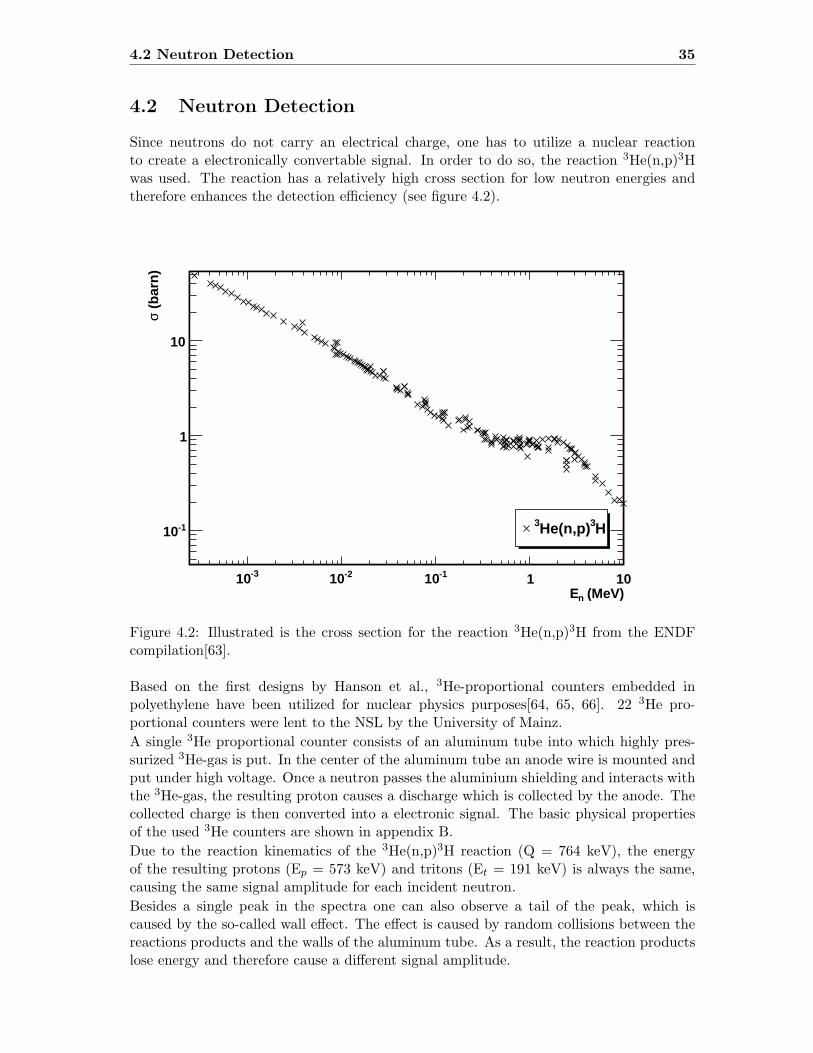
4.2 Neutron Detection 35
4.2 Neutron Detection
Since neutrons do not carry an electrical charge, one has to utilize a nuclear reactionto create a electronically convertable signal. In order to do so, the reaction 3He(n,p)3Hwas used. The reaction has a relatively high cross section for low neutron energies andtherefore enhances the detection efficiency (see figure 4.2).
(MeV)nE
-310 -210 -110 1 10
(ba
rn)
s
-110
1
10
H3He(n,p)3
Figure 4.2: Illustrated is the cross section for the reaction 3He(n,p)3H from the ENDFcompilation[63].
Based on the first designs by Hanson et al., 3He-proportional counters embedded inpolyethylene have been utilized for nuclear physics purposes[64, 65, 66]. 22 3He pro-portional counters were lent to the NSL by the University of Mainz.
A single 3He proportional counter consists of an aluminum tube into which highly pres-surized 3He-gas is put. In the center of the aluminum tube an anode wire is mounted andput under high voltage. Once a neutron passes the aluminium shielding and interacts withthe 3He-gas, the resulting proton causes a discharge which is collected by the anode. Thecollected charge is then converted into a electronic signal. The basic physical propertiesof the used 3He counters are shown in appendix B.
Due to the reaction kinematics of the 3He(n,p)3H reaction (Q = 764 keV), the energyof the resulting protons (Ep = 573 keV) and tritons (Et = 191 keV) is always the same,causing the same signal amplitude for each incident neutron.
Besides a single peak in the spectra one can also observe a tail of the peak, which iscaused by the so-called wall effect. The effect is caused by random collisions between thereactions products and the walls of the aluminum tube. As a result, the reaction productslose energy and therefore cause a different signal amplitude.

36 Experimental Techniques and Procedures
To determine the optimum operating voltage each single 3He tube was tested with differentpreamplifiers at different voltages. An operating voltage of 1400 V was found to be optimal.
4.2.1 Moderation of Neutrons
The cross section of the 3He(n,p)3H reaction increases with lower neutron energies. There-fore, one can increase the detection yield by decreasing the neutron energy before it entersthe 3He proportional counter. This can be achieved by forcing the neutrons to pass throughadditional material in which they lose energy (known as moderation or thermalization)before they reach the 3He counter.Behind the moderation of neutrons stand inelastic scattering processes in a so calledmoderator material. Ideally the neutrons enter the material, loose energy due to severalscattering processes and enter the 3He proportional counter with an energy lower thantheir original energy[67].Concerning the scattering processes, materials with a low Z are favored and should notcause other interactions. Polyethylene and similar (CH)n based materials have been usedas moderation materials in the development of neutron detection systems[68, 69, 70, 71].The advantages are that polyethylene is relatively easy to machine and is not expensive.Theoretically, the moderation of neutrons can be described by the scattering matrix S(α,β)formalism which is used in simulation frameworks to calculate the moderation process :
σ(E → E′, µ) =σb2kT
√E′
ES(α, β) (4.3)
with σb being the material-dependent characteristic bound scattering cross sections and µthe cosine of the scattering angle in the laboratory system. The scattering cross sectionis dependent on momentum (α) and energy (β) transfer :
α =E′ + E − 2
√E′Eµ
AkT, β =
E′ − E
kT(4.4)
where A is the ratio of the scatterer mass to the neutron mass.The moderation method itself introduces the disadvantage that one does not know theinitial neutron energy before the neutron enters the moderation material.
4.2.2 Design Principles
To design a neutron detector based on 3He proportional counters and moderation material,one has to follow certain design principles which are crucial for its performance.The most crucial parameter is the efficiency: the number of detected neutrons per numberof emitted neutrons. Since the expected reaction yields are relatively low, the efficiencyneeds to be maximized and therefore the design of the detector follows primarily thiscriterion.A second criterion is that the neutron detector should have a flat response function fordifferent neutron energies and be relatively position insensitive towards the target position.The idea of an easy adaptability of the system has also been incorporated in the designprocess.For example, the attachment of additional shielding or moderation material was aimed tobe as simple as possible. Another aspect is that the neutron detector should be set up atthe end of a shared beamline so that it can be used for other experiments as well.
4.2 Neutron Detection 37
As a first step in the actual design process, the design of previous neutron detectorsand their performances were reviewed. Measurements of low energy reactions in generaland delayed neutron emission experiments were major applications for such detectionsystems[68, 69, 70, 71].With no natural neutron sources available to deliver neutrons at discrete energies, ex-perimental measurements on nuclear reactions were performed to validate computationalsimulations and derive an efficiency function later on. To ensure an accurate computationalsimulation, it was chosen to design a test detector and measure its response. Later on,the experimental results were compared to the simulations. In the simulations one heavilyrelies on the accuracy of the used scattering and reactions cross sections, the moderationof the neutrons plays a crucial role, since it determines the energy of the neutron whenit enters the proportional counter. With knowledge and correlation between experimentalperformance and computational simulations the final neutron detector was designed andtested.
4.2.3 Computational Simulations
The previously mentioned computational simulations are based on the Monte-Carlo method.The Monte-Carlo method allows to duplicate and model statistical processes such as inter-actions between particles and matter. The modeling process is based on random numberseeds and consists of sequentially modeled processes. For the transport of particles throughmatter it is crucial that the derived code is able to track the particles and their correspond-ing interactions. To determine the outcome of each process step the probability functionsof each interaction are randomly sampled.Experimental data sets for different transport and interaction processes and particles areincluded into the computations to achieve a maximum of accuracy. For additional valida-tion purposes, especially for the physics models used, it was chosen to use two simulationframeworks, GEANT4 and MCNP5[72, 73].
GEANT4
GEANT4 is an object-oriented simulation toolkit primarly delevoped for simulations ofexperiments at the European Nuclear Research Organisation (CERN). The programminglanguage used is C++ with the code being open source. The toolkit provides the necessaryaccessories such as geometry design, physical models, materials etc. for the user to be ableto simulate a full experimental setup.The first choice one has to make is to choose the right physical model for the descriptionof the physical interactions. In order to do so, the interaction between neutrons and 3Hegas was simulated with different models and also compared with experimental data sets.The neutron energies of interest are below 10 MeV, therefore computational simulationswere only performed for initial neutron energies below 10 MeV.It was found that different physical models incorporated in the computational simulationsdelivered (for the same geometry) the same results within less than a percent of deviation.The so called QGSP (Quark-Gluon-String-Plasma) model was finally used, since it isreported to produce the best results of thermal neutron scattering in matter[74].GEANT4 uses also experimental data to model the scattering of thermal neutrons inmatter. The experimental data is derived from evaluated data libraries such as ENDFand JENDL[63, 75]. To ensure a correct handling of the modeling and use of experimentaldata, simple simulations were carried out in which neutrons were directly sent through a

38 Experimental Techniques and Procedures
large volume of 3He gas. The results were then compared to the evaluated data sets ofENDF/B-VI.8 and JENDL3.3.
To achieve a physical meaningful result, the number of recorded reactions must be weightedby the energy loss of the neutron from its starting point to its interaction point with thegas.
In other terms : Two neutrons that have the same initial energy are not necessarilydetected with the same probability, since e.g. scattering causes them to lose differentamounts of energy until they reach their interaction point. At their interaction point theywill have different energies with which they interact with the gas. Therefore, the relevantcross-sections and detection probabilities will be different.
As a consequence, the results were weighted with respect to the ratio of initial energy andthe energy at interaction point. Very good agreement between for example the ENDFdata set, the data set used by GEANT4 and the actual calculated data was achieved (seefigure 4.3).
initial neutron energy (MeV)1 10
cros
s se
ctio
n (a
rb. u
nits
)
-110
1
10
ENDF/B-VII.0
weigthed GEANT4 simulation results
Figure 4.3: Comparison between the experimental data set provided by ENDF and cal-culated by GEANT4. The GEANT4 results were weighted with respect to the ratio ofinitial neutron energy and neutron energy at interaction point.
GEANT4 allows to include a parameter (G4NEUTRONHP SKIP MISSING ISOTOPES )where the modeling of neutron data sets for isotopes not implemented is skipped. Testsshowed, that it had no effect on the results of the experimental setup.
To implement different physical models for the same process, the computation of inter-actions between particles is based on the calculation of the distance from the origin ofthe particle to the point of interaction (or decay). The probability of the particle not
4.2 Neutron Detection 39
interacting with anything within a given distance ℓ is defined as :
P (ℓ) = e−nλ , nλ =
∫ ℓ
0
dℓ
λ(ℓ)(4.5)
where the mean free path λ for interactions in a material of density ρ and the cross sectionσ are defined as:
1
λ= ρ
∑i
xiσimi
(4.6)
with i denoting the different isotopes in the material.
This implies that e.g. exact material densities have to be taken into account in order toachieve an accurate experimental description. For example, the 3He-gas in the simulatedproportional counter has to be described at 10 atm pressure, since the interaction proba-bility between neutron and the 3He-gas is pressure dependent. Note, that the probabilitydistribution can be written as :
nλ = −ln(η) (4.7)
where η is a random number between 0 and 1. Therefore the probability distribution isindependent of energy and material.
Despite a precise description of the experimental geometry, it is also necessary to defineconditions and qualitative measures for the desired quantity. As previously mentioned,the number of detected neutrons per number of emitted neutrons (the efficiency) for eachinitial neutron energy is the key parameter. The number of detected neutrons is equal tothe number of 3He(n,p)3H reactions within the 3He proportional counters.
The neutrons which enter the 3He proportional counters from the surrounding materialwere registered. If the neutron interacts with the 3He gas resulting in a proton and atriton, the event would be registered and recorded. Finally, this was defined within thetracking routines of GEANT4 to ensure a precise count of recorded 3He(n,p)3H reactionscaused by an incoming neutron.
The simulations were carried out and stored within ROOT histograms to be able to judgethe response function of the chosen detector geometry[76]. Tests with different materialsettings and physics models were performed to ensure a maximum of consistency in thedetector performance. For example, it was chosen to vary the density of the moderatormaterial, since polyethylene is available in different densities.
A higher density results in a higher number of scattering partners for the incoming neutronper volume unit. Therefore, an effect on the thermalization process is expected whichresults in a different detector efficiency. Not only different neutron energies but alsoparameter studies on different neutron source and target positions were performed. Withdifferent source positions it was possible to determine the best target position within theneutron detector and probe it for example against misalignments.
After the parameter studies delivered reliable results, the optimal detector geometry deliv-ered by GEANT4 was implemented into MCNP5 and the results from the two simulationswere compared.
MCNP5
As a second simulation toolkit the Monte Carlo N-Particle code (MCNP5) provided by theDiagnostics Application Group at the Los Alamos National Laboratory was chosen[73].MCNP is based on the programming language FORTRAN and in contrast to GEANT4 not
40 Experimental Techniques and Procedures
openly available. Since it is not openly distributed, it is more strict on the user concerningthe use of physics models and other capabilities. The definition of experimental setups,event biasing and output definition is completely different from GEANT4.
For the purpose of this thesis it was particularly interesting to make use of the S(α,β)tables in MCNP which are crucial for low neutron energies. MCNP, similar to GEANT4,uses data libraries such as ENDF and the treatment of particle tracks etc. is very similiar.
MCNP5 utilizes so called tallies within the calculated scenarios. Tallies are quantitiesdefined in MCNP to deliver an useful output for the user. The restriction on tallies isthat they are based on fluences and products or summations in the cross-section libraries.In general, tallies and their functions are dependent on time and energy, normalized perstarting particle.
Despite the absolute result given by MCNP5, a relative error is given in the output toallow the user to assign the results a confidence levels. The estimated relative error givenby MCNP5 is a confidence statement referring only to the precision of the calculationsand not the accuracy.
Tallies were defined which reflect the number of 3He(n,p)3H reactions within the 3Heproportional chambers. The tally used is the so-called F4 tally, which is the track lengthestimate for a flux within a well-defined physical volume :
ϕV =1
V
∫dE
∫dV
∫dt
∫dΩ Ψ(r, Ω, E, t) (4.8)
with Ψ being the angular flux given by the product of particle density n and velocity v :
Ψ(r, Ω, E, t) = vn(r, Ω, E, t) (4.9)
The average particle flux then becomes :
ϕV =1
V
∫dE
∫dV
∫dt
∫dΩ vn(r, Ω, E, t) (4.10)
=1
V
∫dE
∫dV
∫dt vN(r, E, t) (4.11)
=1
V
∫dE
∫dV
∫ds N(r, E, t) (4.12)
by noting that N(r, E, t) is the density of particles while ds is the differential unit of thetrack length vdt.
By multiplying the average fluence from equation 4.10 with the cross section of 3He anda normalization factor the tally then represents the number of produced 3H particles asa result of the 3He(n,p)3H reaction. Normalized over the number of initial neutrons, oneobtains the efficiency. Therefore the results given by MCNP5 are simple to compare withthe GEANT4 results.
4.2.4 Parameter Studies
It was chosen to study the setup of a relatively small test detector before investigatingthe setup of a full detector. 3He proportional counters were embedded into a block ofpolyethylene with a source of neutrons in the center. The number of 3He proportionalcounters was varied between 4 and 8, with the number of detected neutrons increasingwith the number the number of counters.
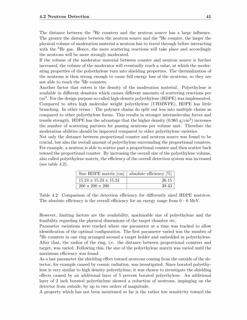
4.2 Neutron Detection 41
The distance between the 3He counters and the neutron source has a large influence.The greater the distance between the neutron source and the 3He counter, the larger thephysical volume of moderation material a neutron has to travel through before interactingwith the 3He gas. Hence, the more scattering reactions will take place and accordinglythe neutrons will be more strongly moderated.If the volume of the moderator material between counter and neutron source is furtherincreased, the volume of the moderator will eventually reach a value, at which the moder-ating properties of the polyethylene turn into shielding properties. The thermalization ofthe neutrons is then strong enough to cause full energy loss of the neutrons, so they arenot able to reach the 3He counters.Another factor that enters is the density of the moderation material. Polyethylene isavailable in different densities which causes different amounts of scattering reactions percm3. For the design purpose so called high-density polyethylene (HDPE) was implemented.Compared to ultra high molecular weight polyethylene (UHMWPE), HDPE has littlebranching. In other terms : The polymer chains do split out less into multiple chains ascompared to other polyethylene forms. This results in stronger intermolecular forces andtensile strength. HDPE has the advantage that the higher density (0.965 g/cm3) increasesthe number of scattering partners for passing neutrons per volume unit. Therefore themoderation abilities should be improved compared to other polyethylene varieties.Not only the distance between proportional counter and neutron source was found to becrucial, but also the overall amount of polyethylene surrounding the proportional counters.For example, a neutron is able to scatter past a proportional counter and then scatter backtoward the proportional counter. By increasing the overall size of the polyethylene volume,also called polyethylene matrix, the efficiency of the overall detection system was increased(see table 4.2).
Size HDPE matrix [cm] absolute efficiency [%]
15.24 x 15.24 x 15.24 26.15
200 x 200 x 200 39.43
Table 4.2: Comparison of the detection efficiency for differently sized HDPE matrices.The absolute efficiency is the overall efficiency for an energy range from 0 - 6 MeV.
However, limiting factors are the availability, machinable size of polyethylene and thefeasibility regarding the physical dimensions of the target chamber etc.Parameter variations were tracked where one parameter at a time was tracked to allowidentification of the optimal configuration. The first parameter varied was the number of3He counters in one ring arranged around a target holder and embedded in polyethylene.After that, the radius of the ring, i.e. the distance between proportional counters andtarget, was varied. Following this, the size of the polyethylene matrix was varied until themaximum efficiency was found.As a last parameter the shielding effect toward neutrons coming from the outside of the de-tector, for example caused by cosmic radiation, was investigated. Since borated polyethy-lene is very similar to high density polyethylene, it was chosen to investigate the shieldingeffects caused by an additional layer of 5 percent borated polyethylene. An additionallayer of 2 inch borated polyethylene showed a reduction of neutrons, impinging on thedetector from outside, by up to two orders of magnitude.A property which has not been mentioned so far is the rather low sensitivity toward the
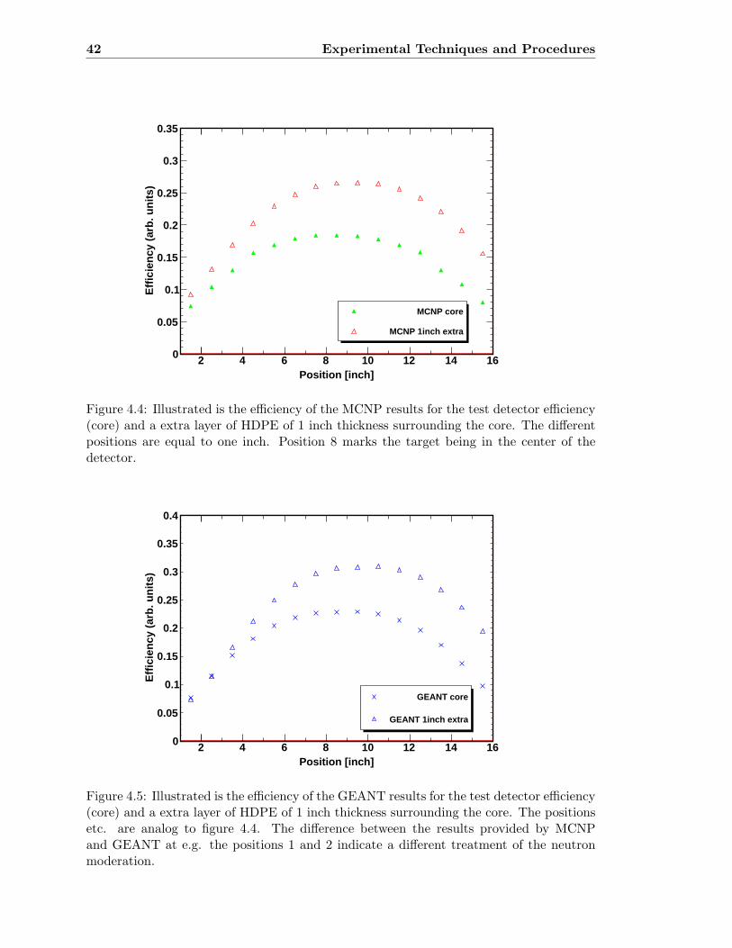
42 Experimental Techniques and Procedures
Position [inch]2 4 6 8 10 12 14 16
Eff
icie
ncy
(ar
b. u
nit
s)
0
0.05
0.1
0.15
0.2
0.25
0.3
0.35
MCNP core
MCNP 1inch extra
Figure 4.4: Illustrated is the efficiency of the MCNP results for the test detector efficiency(core) and a extra layer of HDPE of 1 inch thickness surrounding the core. The differentpositions are equal to one inch. Position 8 marks the target being in the center of thedetector.
Position [inch]2 4 6 8 10 12 14 16
Eff
icie
ncy
(ar
b. u
nit
s)
0
0.05
0.1
0.15
0.2
0.25
0.3
0.35
0.4
GEANT core
GEANT 1inch extra
Figure 4.5: Illustrated is the efficiency of the GEANT results for the test detector efficiency(core) and a extra layer of HDPE of 1 inch thickness surrounding the core. The positionsetc. are analog to figure 4.4. The difference between the results provided by MCNPand GEANT at e.g. the positions 1 and 2 indicate a different treatment of the neutronmoderation.
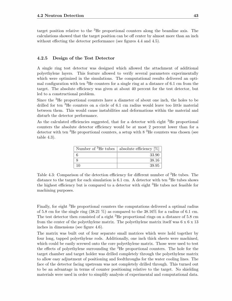
4.2 Neutron Detection 43
target position relative to the 3He proportional counters along the beamline axis. Thecalculations showed that the target position can be off center by almost more than an inchwithout effecting the detector performance (see figures 4.4 and 4.5).
4.2.5 Design of the Test Detector
A single ring test detector was designed which allowed the attachment of additionalpolyethylene layers. This feature allowed to verify several parameters experimentallywhich were optimized in the simulations. The computational results delivered an opti-mal configuration with ten 3He counters for a single ring at a distance of 6.1 cm from thetarget. The absolute efficiency was given at about 40 percent for the test detector, butled to a constructional problem.
Since the 3He proportional counters have a diameter of about one inch, the holes to bedrilled for ten 3He counters on a circle of 6.1 cm radius would leave too little materialbetween them. This would cause instabilities and deformations within the material anddisturb the detector performance.
As the calculated efficiencies suggested, that for a detector with eight 3He proportionalcounters the absolute detector efficiency would be at most 2 percent lower than for adetector with ten 3He proportional counters, a setup with 8 3He counters was chosen (seetable 4.3).
Number of 3He tubes absolute efficiency [%]
6 33.90
8 38.16
10 39.95
Table 4.3: Comparison of the detection efficiency for different number of 3He tubes. Thedistance to the target for each simulation is 6.1 cm. A detector with ten 3He tubes showsthe highest efficiency but is compared to a detector with eight 3He tubes not feasible formachining purposes.
Finally, for eight 3He proportional counters the computations delivered a optimal radiusof 5.8 cm for the single ring (38.21 %) as compared to the 38.16% for a radius of 6.1 cm.The test detector then consisted of a eight 3He proportional rings on a distance of 5.8 cmfrom the center of the polyethylene matrix. The polyethylene matrix itself was 6 x 6 x 13inches in dimensions (see figure 4.6).
The matrix was built out of four separate small matrices which were hold together byfour long, tapped polyethylene rods. Additionally, one inch thick sheets were machined,which could be easily screwed onto the core polyethylene matrix. Those were used to testthe effects of polyethylene surrounding the 3He proportional counters. The hole for thetarget chamber and target holder was drilled completely through the polyethylene matrixto allow easy adjustment of positioning and feedthroughs for the water cooling lines. Theface of the detector facing upstream was not completely drilled through. This turned outto be an advantage in terms of counter positioning relative to the target. No shieldingmaterials were used in order to simplify analysis of experimental and computational data.
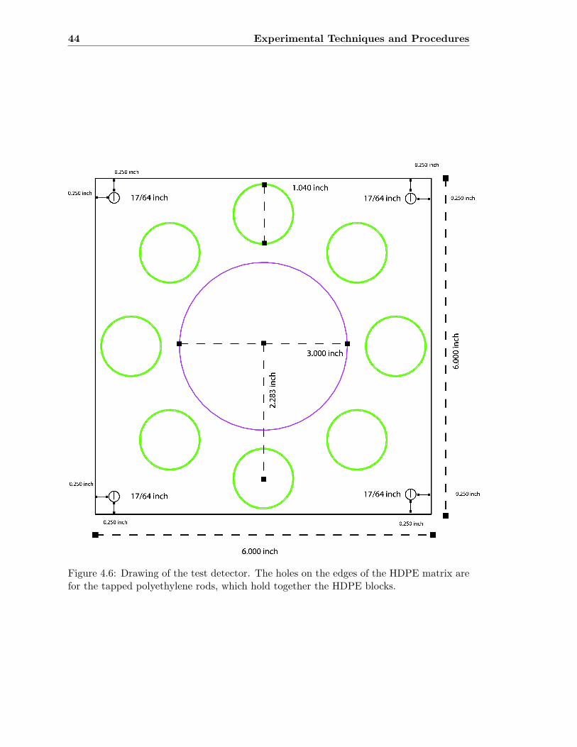
44 Experimental Techniques and Procedures
Figure 4.6: Drawing of the test detector. The holes on the edges of the HDPE matrix arefor the tapped polyethylene rods, which hold together the HDPE blocks.

4.2 Neutron Detection 45
Figure 4.7: Different views of the test detector during the experimental phase.
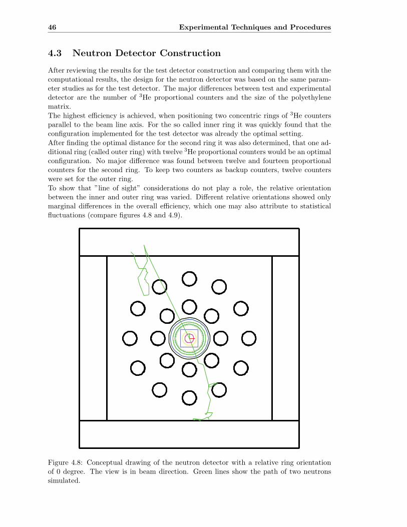
46 Experimental Techniques and Procedures
4.3 Neutron Detector Construction
After reviewing the results for the test detector construction and comparing them with thecomputational results, the design for the neutron detector was based on the same param-eter studies as for the test detector. The major differences between test and experimentaldetector are the number of 3He proportional counters and the size of the polyethylenematrix.
The highest efficiency is achieved, when positioning two concentric rings of 3He countersparallel to the beam line axis. For the so called inner ring it was quickly found that theconfiguration implemented for the test detector was already the optimal setting.
After finding the optimal distance for the second ring it was also determined, that one ad-ditional ring (called outer ring) with twelve 3He proportional counters would be an optimalconfiguration. No major difference was found between twelve and fourteen proportionalcounters for the second ring. To keep two counters as backup counters, twelve counterswere set for the outer ring.
To show that ”line of sight” considerations do not play a role, the relative orientationbetween the inner and outer ring was varied. Different relative orientations showed onlymarginal differences in the overall efficiency, which one may also attribute to statisticalfluctuations (compare figures 4.8 and 4.9).
Figure 4.8: Conceptual drawing of the neutron detector with a relative ring orientationof 0 degree. The view is in beam direction. Green lines show the path of two neutronssimulated.
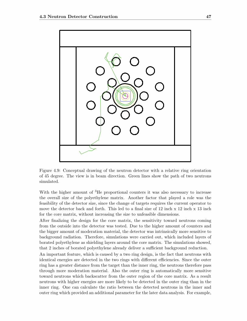
4.3 Neutron Detector Construction 47
Figure 4.9: Conceptual drawing of the neutron detector with a relative ring orientationof 45 degree. The view is in beam direction. Green lines show the path of two neutronssimulated.
With the higher amount of 3He proportional counters it was also necessary to increasethe overall size of the polyethylene matrix. Another factor that played a role was thefeasibility of the detector size, since the change of targets requires the current operator tomove the detector back and forth. This led to a final size of 12 inch x 12 inch x 13 inchfor the core matrix, without increasing the size to unfeasible dimensions.
After finalizing the design for the core matrix, the sensitivity toward neutrons comingfrom the outside into the detector was tested. Due to the higher amount of counters andthe bigger amount of moderation material, the detector was intrinsically more sensitive tobackground radiation. Therefore, simulations were carried out, which included layers ofborated polyethylene as shielding layers around the core matrix. The simulations showed,that 2 inches of borated polyethylene already deliver a sufficient background reduction.
An important feature, which is caused by a two ring design, is the fact that neutrons withidentical energies are detected in the two rings with different efficiencies. Since the outerring has a greater distance from the target than the inner ring, the neutrons therefore passthrough more moderation material. Also the outer ring is automatically more sensitivetoward neutrons which backscatter from the outer region of the core matrix. As a resultneutrons with higher energies are more likely to be detected in the outer ring than in theinner ring. One can calculate the ratio between the detected neutrons in the inner andouter ring which provided an additional parameter for the later data analysis. For example,
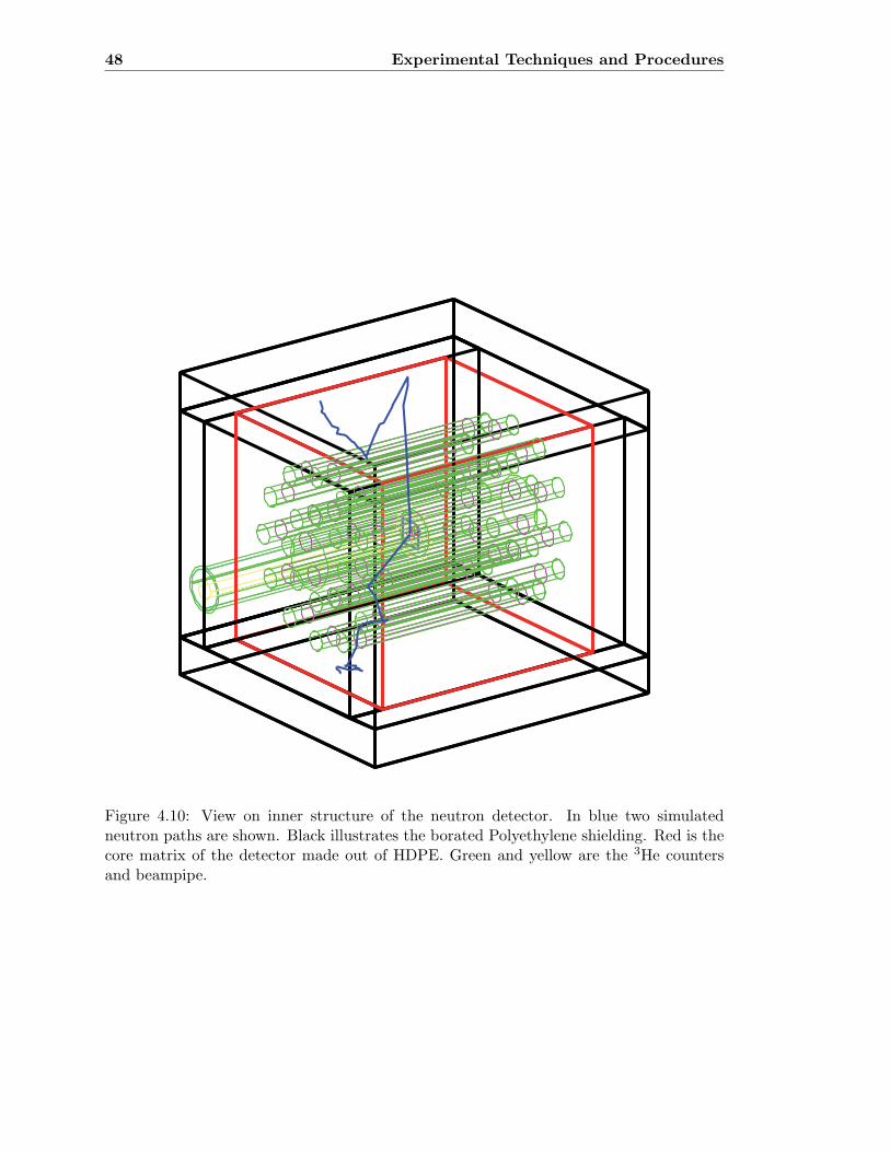
48 Experimental Techniques and Procedures
Figure 4.10: View on inner structure of the neutron detector. In blue two simulatedneutron paths are shown. Black illustrates the borated Polyethylene shielding. Red is thecore matrix of the detector made out of HDPE. Green and yellow are the 3He countersand beampipe.

4.3 Neutron Detector Construction 49
if a reaction releases neutrons with higher energies than 25Mg(α,n)28Si and 26Mg(α,n)29Si,one should be able to observe this by calculating the ratio of of neutrons detected in theinner and outer ring (see section 5.1.3).
The detector was set up on a sliding table to allow easy target exchange and easy positionmeasurements. To ensure that the weight of the cables and the preamplifiers does noteffect the counters and dislocate them, additional polyethylene rods were inserted betweenpreamplifier and proportional counters. Since sixty cables had to be mounted at thebackside of the detector, an additional sheet of borated polyethylene was machined tohold the cables and reduce the force put onto the counters and preamplifiers.
Figure 4.11: Shown is the neutron detector during the construction phase (top) and duringthe experimental phase (bottom).

50 Experimental Techniques and Procedures
4.3.1 Electronics Setup of the Neutron Detectors
3He proportional counters are operated at positive high voltage and deliver a signal whichneeds to be processed at least through two modules to deliver an interpretable signal fora data acquisition system (DAQ) (see fig. 4.12). The first module used is a preamplifier(Module A) which delivers the high voltage directly to the wire inside the counter and alsodelivers the signal to the next module. After that, an amplifier can be used to amplifythe signal to the desired shape and height for the analog to digital converter (ADC). Forthe test detector this electronics setup was utilized. However, for a detector with twentyproportional counters this would have not been feasible.
Instead, the twenty proportional counters were divided into groups of four and their signalsrelayed to a Quad TFA (Module B). The signals were then summed to one signal (ModuleC). After that, the summed signal were processed through an amplifier (Module D) andrelayed to an ADC (Module E). Additionally, the group sum signals were also summed up(Module F) to deliver a hardware summed signal of the inner and the outer ring. Thosewere then relayed to separate ADCs. Therefore it was possible to observe online the ratiobetween the signals coming into the five different groups and the inner and outer ring.
A B C D E
F
CBA D E
ED
Figure 4.12: Schematic view of the neutron detector electronics for the inner ring. Theelectronics for the outer ring are the same with additional four 3He tubes.Module A : 2003BT Preamplifier; Module B : Ortec 863 Quad TFA; Module C : Phillips740 Fan IN/OUT; Module D : Ortec 552 Amplifier; Module E : ADC; Module F : Phillips740 Fan IN/OUT to sum different groups or rings.
4.3.2 Validation of Computational Calculations
An important factor in the use of computational calculations is the validation of thecomputational results in accordance with experimental results. To ensure a high level ofreliability, it was chosen to validate the calculations in a separate manner.

4.3 Neutron Detector Construction 51
To be able to validate the most important parameters, such as efficiency and positionsensitivity, it was chosen to make use of nuclear reactions which would serve as discreteneutron sources. This allows also to set up the complete detection system as it would beused later on in the experiment and test it towards practicality and gain experience in theoperation of the set up.Besides for accelerator calibration purposes (see section 4.1 ) the reaction 51V(p,n)51Crhas been used in studies of neutron detector performances and is relatively well known[77, 78, 79]. A useful property of the reaction is, that the produced isotope 51Cr hasa relatively long half-life (t 1
2=27.7d). Therefore, its decay to the ground-state can be
conveniently measured after irradiation of a 51V-target. By the detection of the promptneutrons and the gamma activity one is able to determine the absolute efficiency of theneutron detection system via the activation method[27].
52 Experimental Techniques and Procedures
4.4 Counting Station
For decay measurements of the activated 51V-targets a counting station based on a HPGedetector was built. The counting station consisted of a HPGe detector whose Ge crystalwas surrounded by Pb bricks. The Pb bricks were used to reduce room background. Toensure, that between measurements, sample positioning and therefore the efficiency of thedetector was not changed, a sample holder was constructed. The sample holder, mountedon the Al case of the Ge crystal, allowed to measure the efficiency of the detection systemwith different samples at reproducible positions.Since 51Cr decays via a single γ-decay, the efficiency at the energy of the released γ-ray (Eγ
= 320 keV) is crucial. By measuring the efficiency of the detector with a calibrated 133Basource, the efficiency could be determined experimentally at 302 keV, 356 and 383 keV.Summation effects were corrected by measurements with a single γ-ray source at differentdistances. After the experimental determinations, the efficiency at 320 keV was inter-polated to be 8%. The efficiency measurements were repeated before each experimentalbeam time and by different experimentators.
4.5 (p,γ)-Measurement Setup
The thickness measurements via resonances of 18O, 25Mg and 26Mg were performed beforeand after the measurement of each target (see figure 4.13). The γ-rays were detected witha second germanium detector positioned at 90 degrees relative to the target chamber. Theneutron detector was removed so that the germanium detector could be positioned as closeas possible to the target. The crucial parameter of this setup was the reproducibility ofthe detector position and not the efficiency.After the (p,γ) measurements, the Ge detector was moved as far away as possible to avoidneutron damage of the Ge crystal.
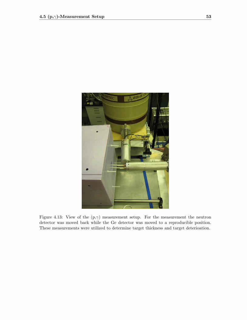
4.5 (p,γ)-Measurement Setup 53
Figure 4.13: View of the (p,γ) measurement setup. For the measurement the neutrondetector was moved back while the Ge detector was moved to a reproducible position.These measurements were utilized to determine target thickness and target deterioation.
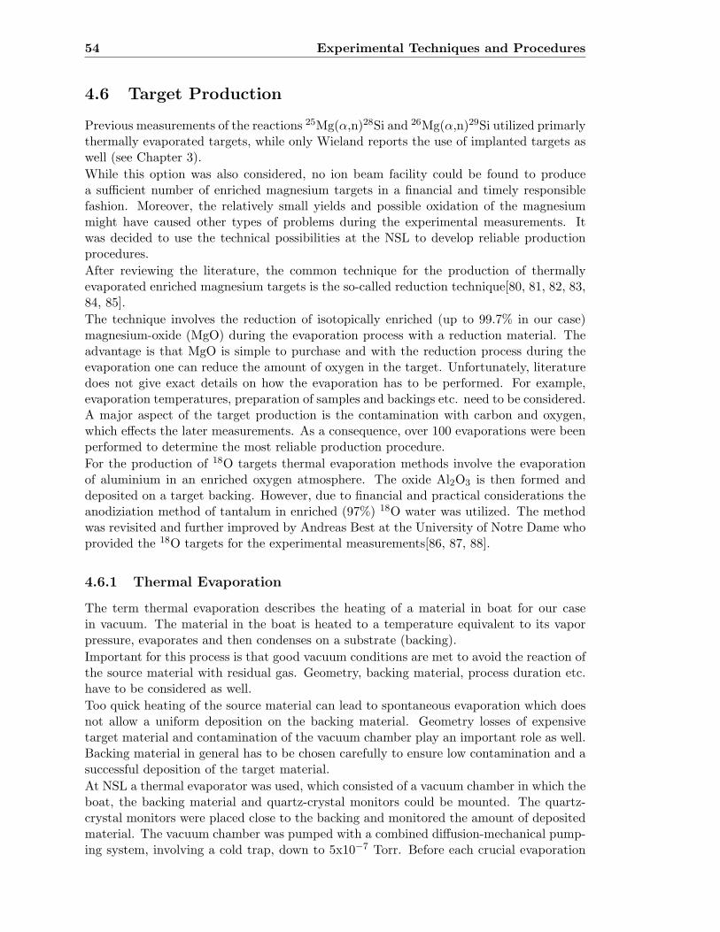
54 Experimental Techniques and Procedures
4.6 Target Production
Previous measurements of the reactions 25Mg(α,n)28Si and 26Mg(α,n)29Si utilized primarlythermally evaporated targets, while only Wieland reports the use of implanted targets aswell (see Chapter 3).
While this option was also considered, no ion beam facility could be found to producea sufficient number of enriched magnesium targets in a financial and timely responsiblefashion. Moreover, the relatively small yields and possible oxidation of the magnesiummight have caused other types of problems during the experimental measurements. Itwas decided to use the technical possibilities at the NSL to develop reliable productionprocedures.
After reviewing the literature, the common technique for the production of thermallyevaporated enriched magnesium targets is the so-called reduction technique[80, 81, 82, 83,84, 85].
The technique involves the reduction of isotopically enriched (up to 99.7% in our case)magnesium-oxide (MgO) during the evaporation process with a reduction material. Theadvantage is that MgO is simple to purchase and with the reduction process during theevaporation one can reduce the amount of oxygen in the target. Unfortunately, literaturedoes not give exact details on how the evaporation has to be performed. For example,evaporation temperatures, preparation of samples and backings etc. need to be considered.A major aspect of the target production is the contamination with carbon and oxygen,which effects the later measurements. As a consequence, over 100 evaporations were beenperformed to determine the most reliable production procedure.
For the production of 18O targets thermal evaporation methods involve the evaporationof aluminium in an enriched oxygen atmosphere. The oxide Al2O3 is then formed anddeposited on a target backing. However, due to financial and practical considerations theanodiziation method of tantalum in enriched (97%) 18O water was utilized. The methodwas revisited and further improved by Andreas Best at the University of Notre Dame whoprovided the 18O targets for the experimental measurements[86, 87, 88].
4.6.1 Thermal Evaporation
The term thermal evaporation describes the heating of a material in boat for our casein vacuum. The material in the boat is heated to a temperature equivalent to its vaporpressure, evaporates and then condenses on a substrate (backing).
Important for this process is that good vacuum conditions are met to avoid the reaction ofthe source material with residual gas. Geometry, backing material, process duration etc.have to be considered as well.
Too quick heating of the source material can lead to spontaneous evaporation which doesnot allow a uniform deposition on the backing material. Geometry losses of expensivetarget material and contamination of the vacuum chamber play an important role as well.Backing material in general has to be chosen carefully to ensure low contamination and asuccessful deposition of the target material.
At NSL a thermal evaporator was used, which consisted of a vacuum chamber in which theboat, the backing material and quartz-crystal monitors could be mounted. The quartz-crystal monitors were placed close to the backing and monitored the amount of depositedmaterial. The vacuum chamber was pumped with a combined diffusion-mechanical pump-ing system, involving a cold trap, down to 5x10⁻⁷ Torr. Before each crucial evaporation
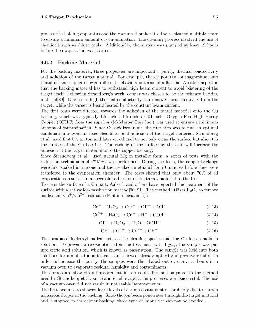
4.6 Target Production 55
process the holding apparatus and the vacuum chamber itself were cleaned multiple timesto ensure a minimum amount of contamination. The cleaning process involved the use ofchemicals such as dilute acids. Additionally, the system was pumped at least 12 hoursbefore the evaporation was started.
4.6.2 Backing Material
For the backing material, three properties are important : purity, thermal conductivityand adhesion of the target material. For example, the evaporation of magnesium ontotantalum and copper showed different behaviors in terms of adhesion. Another aspect isthat the backing material has to withstand high beam current to avoid blistering of thetarget itself. Following Strandberg’s work, copper was chosen to be the primary backingmaterial[89]. Due to its high thermal conductivity, Cu removes heat effectively from thetarget, while the target is being heated by the constant beam current.The first tests were directed towards the adhesion of the target material onto the Cubacking, which was typically 1.5 inch x 1.5 inch x 0.04 inch. Oxygen Free High PurityCopper (OFHC) from the supplier (McMaster Carr Inc.) was used to ensure a minimumamount of contamination. Since Cu oxidizes in air, the first step was to find an optimalcombination between surface cleanliness and adhesion of the target material. Strandberget al. used first 5% aceton and later on ethanol to not only clean the surface but also etchthe surface of the Cu backing. The etching of the surface by the acid will increase theadhesion of the target material onto the copper backing.Since Strandberg et al. used natural Mg in metallic form, a series of tests with thereduction technique and natMgO was performed. During the tests, the copper backingswere first soaked in acetone and then soaked in ethanol for 20 minutes before they weretransfered to the evaporation chamber. The tests showed that only about 70% of allevaporations resulted in a successful adhesion of the target material to the Cu.To clean the surface of a Cu part, Aalseth and others have reported the treatment of thesurface with a activation-passivation method[90, 91]. The method utilizes H2O2 to removeoxides and Cu+/Cu2+ residuals (Fenton mechanism) :
Cu+ +H2O2 → Cu2+ +OH− +OH · (4.13)
Cu2+ +H2O2 → Cu+ +H+ +OOH · (4.14)
OH · +H2O2 → H2O+OOH · (4.15)
OH · +Cu+ → Cu2+ +OH− (4.16)
The produced hydroxyl radical acts as the cleaning species and the Cu ions remain insolution. To prevent a re-oxidation after the treatment with H2O2, the sample was putinto citric acid solution, which is known as passivation. The sample was held into bothsolutions for about 20 minutes each and showed already optically impressive results. Inorder to increase the purity, the samples were then baked out over several hours in avacuum oven to evaporate residual humidity and contaminants.This procedure showed an improvement in terms of adhesion compared to the methodused by Strandberg et al. since almost all evaporation processes were successful. The useof a vacuum oven did not result in noticeable improvements.The first beam tests showed large levels of carbon contaminaton, probably due to carboninclusions deeper in the backing. Since the ion beam penetrates through the target materialand is stopped in the copper backing, those type of impurities can not be avoided.

56 Experimental Techniques and Procedures
An improvement in terms of impurities is the use of gold-plated copper disks[45, 92].OFHC disks are put into an electroplating bath and are then coated with an Au layer. Toavoid diffusion of the gold into the copper, a 1µm thick nickel layer was plated onto thecopper first. To stop the α-beam in the Au layer and not in the Ni or Cu layer, a sufficientlythick layer of Au is necessary. Calculations were performed in which the implantation ofα-particles into Au was simulated. For this purpose the software SRIM2008 was used([93], also see http://www.srim.org).
The calculations showed that for a maximum beam energy of Eα = 3 MeV a 5µm layer ofAu would be sufficient to stop the beam. The OFHC disks were obtained by GoodfellowInc. corporation while the electrochemical plating was performed at the Max-Planck-Institut fur Chemie (MPIC).
The Au plated copper disks were also treated by the activation-passivation method, forseveral minutes, and then directly transferred to the evaporation chamber. In terms ofadhesion they showed a perfect behaviour and turned out to be the backings with the leastcontamination.
4.6.3 Evaporation Process
In literature, the evaporation process of MgO being reduced to Mg includes a mixture ofMgO with a material that reduces MgO during the process.
Tests with tantalum, zirconium and titanium showed, that Ta is the preferred reductionmaterial, since it showed no difficulties in handling and processing. To reduce costs andcontamination of the evaporation chamber, the amount needed for the evaporation processwas first determined by weighing the MgO and the Ta before mixing it.
The amount of tantalum used is critical for the reduction process. The amount of oxygendeposited on the target backings could be reduced by simply increasing the amount of Tan-talum compared to a fixed amount of MgO. This was shown with the RBS measurementsas well. The reduction process can be described as :
10 MgO + 4 Ta → 10 Mg + 2 Ta2O5 (4.17)
and therefore it can be concluded that, with an increased amount of reduction partners, thereduction process can be more effective. It was found to be optimal to have an absolutemass ratio of 25:1 for Ta:MgO. MgO amounts of 15 mg were sufficient for one targetproduction process.
Several tests with different heating sources (boats) were also conducted. Boats come indifferent materials and shapes. Boats made out of tantalum can only reach temperaturesup to 1600 C while boats made out of tungsten could reach temperatures up to 1800C. This is critical since no exact evaporation temperature (or vapor pressure) has beenreported for the reduction process and boat breakdowns were observed during the firsttest. Therefore, the first series of tests conducted included the use of so called dimpleboats made out of tantalum, tungsten and molybdenum (see figures 4.14 and 4.15).
Surprisingly, the molybdenum boats showed the best results in achieving an evaporation.This was possibly also enhanced by the molybdenum itself, since it can reduce MgO byitself as well[94].
A different aspect is the surface contact between the MgO, Ta and the boat. It was firstincreased by using a few drops of water and mix the MgO and Ta in the boat itself. Un-fortunately, during the heating process the water evaporates suddenly and the mixture
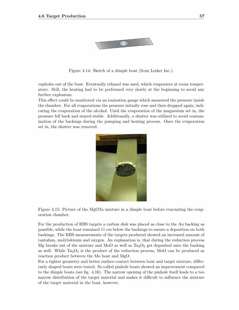
4.6 Target Production 57
Figure 4.14: Sketch of a dimple boat (from Lesker Inc.).
explodes out of the boat. Eventually ethanol was used, which evaporates at room temper-ature. Still, the heating had to be performed very slowly at the beginning to avoid anyfurther explosions.
This effect could be monitored via an ionization gauge which measured the pressure insidethe chamber. For all evaporations the pressure initially rose and then dropped again, indi-cating the evaporation of the alcohol. Until the evaporation of the magnesium set in, thepressure fell back and stayed stable. Additionally, a shutter was utilized to avoid contam-ination of the backings during the pumping and heating process. Once the evaporationset in, the shutter was removed.
Figure 4.15: Picture of the MgOTa mixture in a dimple boat before evacuating the evap-oration chamber.
For the production of RBS targets a carbon disk was placed as close to the Au backing aspossible, while the boat remained 11 cm below the backings to ensure a deposition on bothbackings. The RBS measurements of the targets produced showed an increased amount oftantalum, molybdenum and oxygen. An explanation is, that during the reduction processMg breaks out of the mixture and MoO as well as Ta2O5 get deposited onto the backingas well. While Ta2O5 is the product of the reduction process, MoO can be produced asreaction product between the Mo boat and MgO.
For a tighter geometry and better surface contact between boat and target mixture, differ-ently shaped boats were tested. So called pinhole boats showed an improvement comparedto the dimple boats (see fig. 4.16). The narrow opening of the pinhole itself leads to a toonarrow distribution of the target material and makes it difficult to influence the mixtureof the target material in the boat, however.
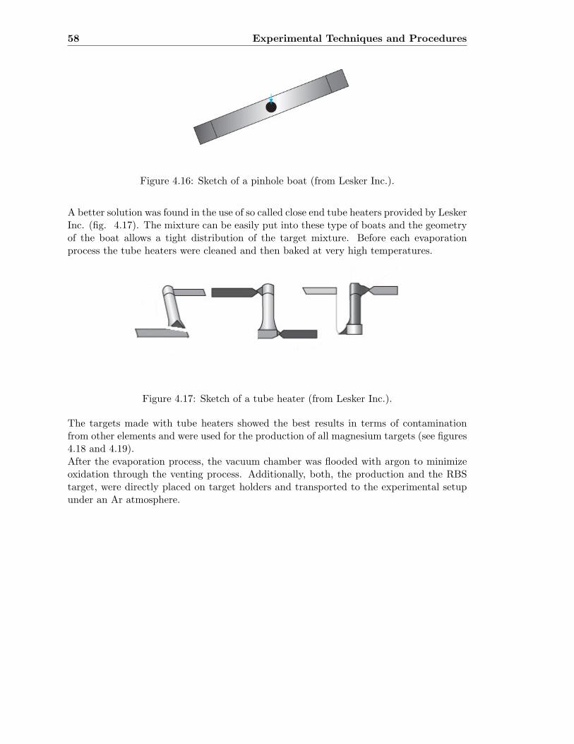
58 Experimental Techniques and Procedures
Figure 4.16: Sketch of a pinhole boat (from Lesker Inc.).
A better solution was found in the use of so called close end tube heaters provided by LeskerInc. (fig. 4.17). The mixture can be easily put into these type of boats and the geometryof the boat allows a tight distribution of the target mixture. Before each evaporationprocess the tube heaters were cleaned and then baked at very high temperatures.
Figure 4.17: Sketch of a tube heater (from Lesker Inc.).
The targets made with tube heaters showed the best results in terms of contaminationfrom other elements and were used for the production of all magnesium targets (see figures4.18 and 4.19).After the evaporation process, the vacuum chamber was flooded with argon to minimizeoxidation through the venting process. Additionally, both, the production and the RBStarget, were directly placed on target holders and transported to the experimental setupunder an Ar atmosphere.

4.6 Target Production 59
Figure 4.18: Picture of a Mg target after evaporation.
4.6.4 Vanadium Targets
For the activation measurements a series of vanadium targets were produced. The evapo-ration of vanadium compared to magnesium oxide is relatively simple. The vanadium canbe placed in a tungsten dimple boat and then heated until it evaporates onto a previouslybaked Ta backing. Since vanadium has a high vapor pressure, it is important to have goodsurface contact between vanadium and the boat to ensure that the heat is well-distributed.

60 Experimental Techniques and Procedures
Figure 4.19: Picture of the evaporation setup within the evaporation chamber. Shown arethe AuNiCu and RBS backing mounted next to each other. The shutter is in the ”closed”position to avoid contamination, while the tube heater is mounted on the current leads.
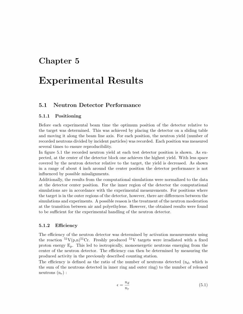
Chapter 5
Experimental Results
5.1 Neutron Detector Performance
5.1.1 Positioning
Before each experimental beam time the optimum position of the detector relative tothe target was determined. This was achieved by placing the detector on a sliding tableand moving it along the beam line axis. For each position, the neutron yield (number ofrecorded neutrons divided by incident particles) was recorded. Each position was measuredseveral times to ensure reproducibility.
In figure 5.1 the recorded neutron yield at each test detector position is shown. As ex-pected, at the center of the detector block one achieves the highest yield. With less spacecovered by the neutron detector relative to the target, the yield is decreased. As shownin a range of about 4 inch around the center position the detector performance is notinfluenced by possible misalignments.
Additionally, the results from the computational simulations were normalized to the dataat the detector center position. For the inner region of the detector the computationalsimulations are in accordance with the experimental measurements. For positions wherethe target is in the outer regions of the detector, however, there are differences between thesimulations and experiments. A possible reason is the treatment of the neutron moderationat the transition between air and polyethylene. However, the obtained results were foundto be sufficient for the experimental handling of the neutron detector.
5.1.2 Efficiency
The efficiency of the neutron detector was determined by activation measurements usingthe reaction 51V(p,n)51Cr. Freshly produced 51V targets were irradiated with a fixedproton energy Ep. This led to isotropically, monoenergetic neutrons emerging from thecenter of the neutron detector. The efficiency can then be determined by measuring theproduced activity in the previously described counting station.
The efficiency is defined as the ratio of the number of neutrons detected (nd, which isthe sum of the neutrons detected in inner ring and outer ring) to the number of releasedneutrons (nr) :
ϵ =nd
nr(5.1)
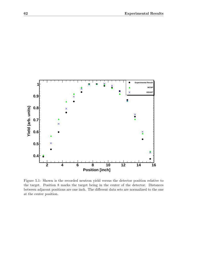
62 Experimental Results
Position [inch]2 4 6 8 10 12 14 16
Yie
ld (
arb
. un
its)
0.4
0.5
0.6
0.7
0.8
0.9
1Experimental Result
MCNP
GEANT
Figure 5.1: Shown is the recorded neutron yield versus the detector position relative tothe target. Position 8 marks the target being in the center of the detector. Distancesbetween adjacent positions are one inch. The different data sets are normalized to the oneat the center position.

5.1 Neutron Detector Performance 63
The number of neutrons detected was measured promptly and was corrected for back-ground radiation and dead time effects, while the number of released neutrons is equal tothe number of produced 51Cr nuclei. The number of 51Cr nuclei produced and thereforethe number of released neutrons was determined in turn, by measuring the activity of theactivated 51V target. The number of 51Cr produced in a single activation (Ni); and (still)present a some t is given by :
Ni =ki ·Pλ
(1− e−λ · ts) · e−λ · (t−te) (5.2)
Here λ is the decay constant and P the production rate. ts represents the start time ofthe activation and te the end time. The factor ki is a correction factor for possible targetdepletion and beam current deviations. It was determined by calculating the neutron yieldafter each activation period. Each 51V target was irriadiated multiple times, to be able tomonitor the data online and to be able to react e.g. to target deterioation. The index idenotes multiple activation intervals for one 51V target.
The production rate P was determined via the measurement of the produced 51Cr nuclei.The number of emitted γ-rays (Nγ) from the 51Cr nuclei during a defined time interval isgiven by :
Nγ =Nc
I · ϵGe ·DT(5.3)
with Nc being the number of recorded γ-rays, I the branching ratio, ϵGe the efficiency ofthe Germanium detector and DT the dead time correction.
Nγ is simply the difference of the number of 51Cr nuclei at the beginning (Ni(tAS)) andthe end (Ni(tAE)) of the measurement. This leads then to :∑
i
(Ni(tAS)−Ni(tAE)) =Nc
I · ϵGe ·DT(5.4)
Inserting equation 5.2 into equation 5.4 results in :
Nc
I · ϵGe ·DT=∑i
(ki ·Pλ
(1−e−λ · ts) · e−λ · (tAS−te)− ki ·Pλ
(1−e−λ · ts) · e−λ · (tAE−te)) (5.5)
By assuming that the production rate is constant for each activation interval, equation5.5 can be transformed to :
P =Nc
I · ϵGe ·DT· λ∑
i ki · (1− e−λ · ts) · (e−λ · (tAS−te) − e−λ · (tAE−te)))(5.6)
Multiplying the production rate with the activation time tA results in the number ofneutrons released over each activation interval. Hence, the efficiency can be expressed as :
ϵ =nd
P · tA(5.7)
By inserting equation 5.6 into equation 5.7 one then calculates the efficiency for a singleneutron energy.
The determination of the efficiency at neutron energies higher than 650 keV was notpossible due to very high dead time effects in the detection system.
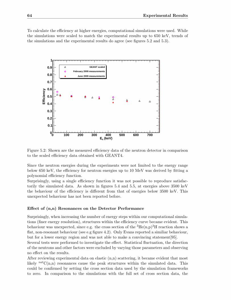
64 Experimental Results
To calculate the efficiency at higher energies, computational simulations were used. Whilethe simulations were scaled to match the experimental results up to 650 keV, trends ofthe simulations and the experimental results do agree (see figures 5.2 and 5.3).
(keV)nE0 100 200 300 400 500 600 700
Eff
icie
ncy
0
0.1
0.2
0.3
0.4
0.5
0.6
0.7
0.8
0.9
1
GEANT scaled
February 2009 measurements
June 2009 measurements
Figure 5.2: Shown are the measured efficiency data of the neutron detector in comparisonto the scaled efficiency data obtained with GEANT4.
Since the neutron energies during the experiments were not limited to the energy rangebelow 650 keV, the efficiency for neutron energies up to 10 MeV was derived by fitting apolynomial efficiency function.
Surprisingly, using a single efficiency function it was not possible to reproduce satisfac-torily the simulated data. As shown in figures 5.4 and 5.5, at energies above 3500 keVthe behaviour of the efficiency is different from that of energies below 3500 keV. Thisunexpected behaviour has not been reported before.
Effect of (n,n) Resonances on the Detector Performance
Surprisingly, when increasing the number of energy steps within our computational simula-tions (finer energy resolution), structures within the efficiency curve became evident. Thisbehaviour was unexpected, since e.g. the cross section of the 3He(n,p)3H reaction shows aflat, non-resonant behaviour (see e.g figure 4.2). Only Evans reported a similiar behaviour,but for a lower energy region and was not able to make a convincing statement[95].
Several tests were performed to investigate the effect. Statistical fluctuation, the directionof the neutrons and other factors were excluded by varying those parameters and observingno effect on the results.
After reviewing experimental data on elastic (n,n) scattering, it became evident that mostlikely natC(n,n) resonances cause the peak structures within the simulated data. Thiscould be confirmed by setting the cross section data used by the simulation frameworksto zero. In comparison to the simulations with the full set of cross section data, the
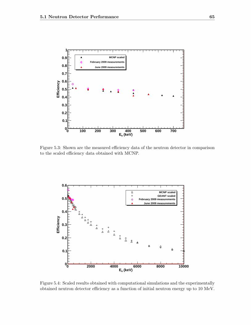
5.1 Neutron Detector Performance 65
(keV)nE0 100 200 300 400 500 600 700
Eff
icie
ncy
0
0.1
0.2
0.3
0.4
0.5
0.6
0.7
0.8
0.9
1
MCNP scaled
February 2009 measurements
June 2009 measurements
Figure 5.3: Shown are the measured efficiency data of the neutron detector in comparisonto the scaled efficiency data obtained with MCNP.
(keV)nE0 2000 4000 6000 8000 10000
Eff
icie
ncy
0
0.1
0.2
0.3
0.4
0.5
0.6
MCNP scaledGEANT scaled
February 2009 measurements
June 2009 measurements
Figure 5.4: Scaled results obtained with computational simulations and the experimentallyobtained neutron detector efficiency as a function of initial neutron energy up to 10 MeV.
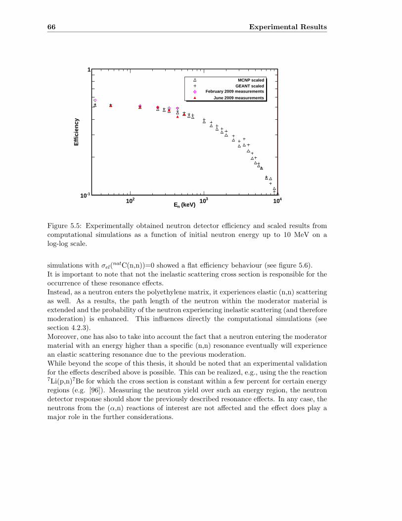
66 Experimental Results
(keV)nE210 310 410
Effi
cien
cy
-110
1
MCNP scaledGEANT scaled
February 2009 measurements
June 2009 measurements
Figure 5.5: Experimentally obtained neutron detector efficiency and scaled results fromcomputational simulations as a function of initial neutron energy up to 10 MeV on alog-log scale.
simulations with σel(natC(n,n))=0 showed a flat efficiency behaviour (see figure 5.6).
It is important to note that not the inelastic scattering cross section is responsible for theoccurrence of these resonance effects.Instead, as a neutron enters the polyethylene matrix, it experiences elastic (n,n) scatteringas well. As a results, the path length of the neutron within the moderator material isextended and the probability of the neutron experiencing inelastic scattering (and thereforemoderation) is enhanced. This influences directly the computational simulations (seesection 4.2.3).Moreover, one has also to take into account the fact that a neutron entering the moderatormaterial with an energy higher than a specific (n,n) resonance eventually will experiencean elastic scattering resonance due to the previous moderation.While beyond the scope of this thesis, it should be noted that an experimental validationfor the effects described above is possible. This can be realized, e.g., using the the reaction7Li(p,n)7Be for which the cross section is constant within a few percent for certain energyregions (e.g. [96]). Measuring the neutron yield over such an energy region, the neutrondetector response should show the previously described resonance effects. In any case, theneutrons from the (α,n) reactions of interest are not affected and the effect does play amajor role in the further considerations.
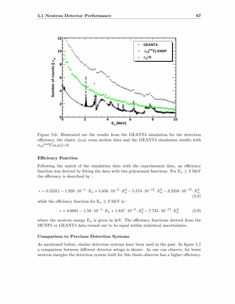
5.1 Neutron Detector Performance 67
(MeV)nE0 2 4 6 8 10
elsN
um
ber
of
cou
nts
||
0
2
4
6
8
10
12
GEANT4
C) ENDFnat(els
=0els
Figure 5.6: Illustrated are the results from the GEANT4 simulation for the detectionefficiency, the elastic (n,n) cross section data and the GEANT4 simulation results withσel(
natC(n,n))=0.
Efficiency Function
Following the match of the simulation data with the experimental data, an efficiencyfunction was derived by fitting the data with two polynomial functions. For En ≤ 3 MeVthe efficiency is described by :
ϵ = 0.52311− 1.928 · 10−4 ·En + 5.856 · 10−8 ·E2n − 5.574 · 10−12 ·E3
n − 3.2358 · 10−15 ·E4n
(5.8)while the efficiency function for En ≥ 3 MeV is :
ϵ = 0.6081− 1.58 · 10−4 ·En + 1.847 · 10−8 ·E2n − 7.745 · 10−13 ·E3
n (5.9)
where the neutron energy En is given in keV. The efficiency functions derived from theMCNP5 or GEANT4 data turned out to be equal within statistical uncertainties.
Comparison to Previous Detection Systems
As mentioned before, similar detection systems have been used in the past. In figure 5.7a comparison between different detector setups is shown. As one can observe, for lowerneutron energies the detection system built for this thesis observes has a higher efficiency.
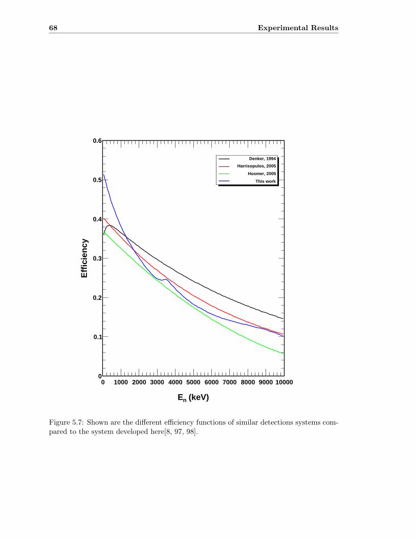
68 Experimental Results
(keV)nE
0 1000 2000 3000 4000 5000 6000 7000 8000 9000 10000
Eff
icie
ncy
0
0.1
0.2
0.3
0.4
0.5
0.6
Denker, 1994
Harrisopulos, 2005
Hosmer, 2005
This work
Figure 5.7: Shown are the different efficiency functions of similar detections systems com-pared to the system developed here[8, 97, 98].

5.1 Neutron Detector Performance 69
5.1.3 Ring Ratio
The ring ratio (R) is defined as the ratio between the number of counts detected withinthe inner ring (NIR) and the number of counts within the outer ring (NOR):
R =NIR
NOR(5.10)
The number of detected neutrons within each ring is dependent on the initial neutronenergy. The higher the initial neutron energy, the longer the path through the moderatormaterial. Consequently, the ring ratio can be used as a tool to roughly estimate the initialneutron energy.The ring ratio was calculated from the efficiency measurements and compared to theresults of the computational simulations (see figure 5.8). The efficiency for each neutronenergy can then be assigned to a specific initial neutron energy as well (see figure 5.10).
Ratio IR/OR0.6 0.8 1 1.2 1.4 1.6 1.8 2
Eff
icie
ncy
0
0.1
0.2
0.3
0.4
0.5
0.6
0.7
0.8
0.9
1
MCNP scaled
February 2009 measurements
June 2009 measurements
Figure 5.8: Plotted is the effciency of the neutron detector as a function of the ring ratio.The results obtained with MCNP provide the best match to the experimental data.
The nature of (α,n) reactions as two step processes involves also the occurrence of so-calledneutron groups. A neutron group ni describes the neutrons who populate the ith stateof the final nucleus. Neutrons belonging to different groups have different energies (seefigure 5.9). This results in a neutron detection efficiency that is different for each neutrongroup. This can be corrected for by analyzing the ring ratios and determining the neutrongroups. A function for the neutron energy was derived by fitting the data displayed infigures 5.10 and 5.11 :
En(R) = e(11.42−3.762∗R) (5.11)
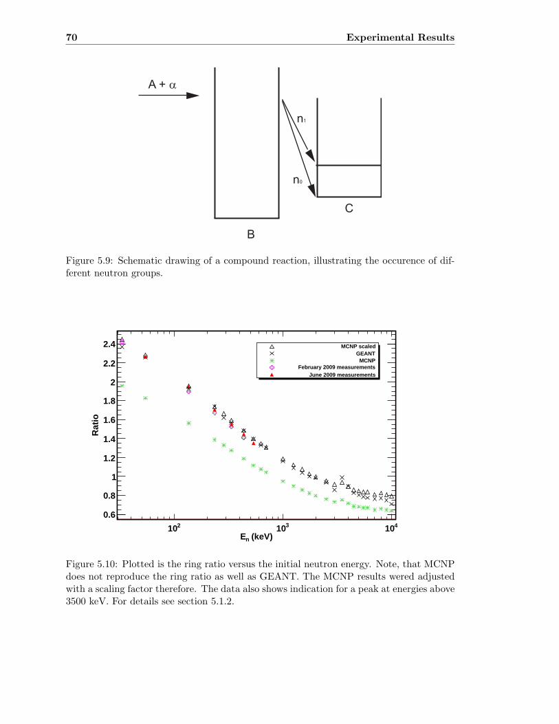
70 Experimental Results
A + α
B
C
n1
n0
Figure 5.9: Schematic drawing of a compound reaction, illustrating the occurence of dif-ferent neutron groups.
(keV)nE210 310 410
Rat
io
0.6
0.8
1
1.2
1.4
1.6
1.8
2
2.2
2.4 MCNP scaledGEANT
MCNPFebruary 2009 measurements
June 2009 measurements
Figure 5.10: Plotted is the ring ratio versus the initial neutron energy. Note, that MCNPdoes not reproduce the ring ratio as well as GEANT. The MCNP results wered adjustedwith a scaling factor therefore. The data also shows indication for a peak at energies above3500 keV. For details see section 5.1.2.
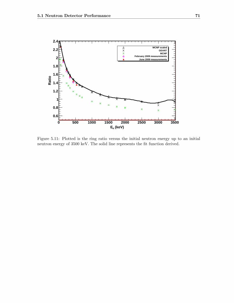
5.1 Neutron Detector Performance 71
(keV)nE0 500 1000 1500 2000 2500 3000 3500
Rat
io
0.6
0.8
1
1.2
1.4
1.6
1.8
2
2.2
2.4
MCNP scaledGEANT
MCNPFebruary 2009 measurements
June 2009 measurements
Figure 5.11: Plotted is the ring ratio versus the initial neutron energy up to an initialneutron energy of 3500 keV. The solid line represents the fit function derived.
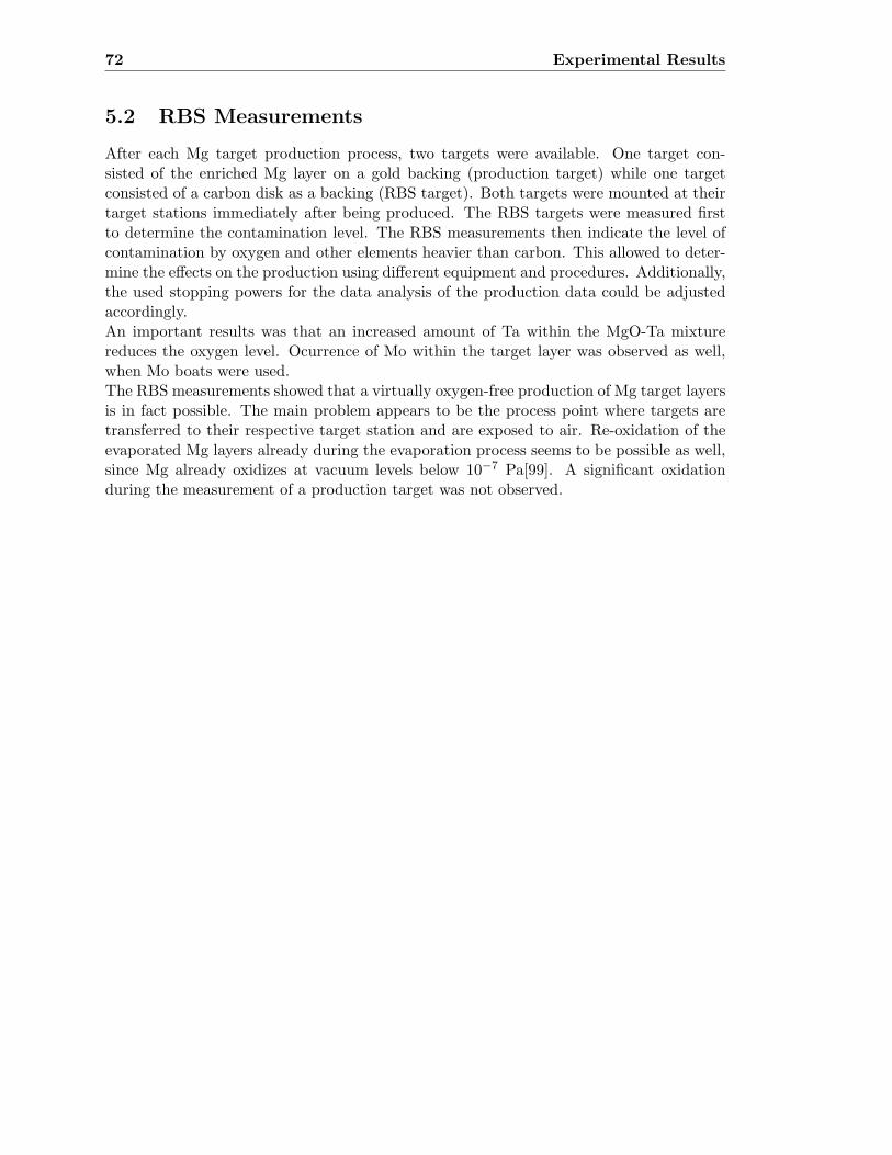
72 Experimental Results
5.2 RBS Measurements
After each Mg target production process, two targets were available. One target con-sisted of the enriched Mg layer on a gold backing (production target) while one targetconsisted of a carbon disk as a backing (RBS target). Both targets were mounted at theirtarget stations immediately after being produced. The RBS targets were measured firstto determine the contamination level. The RBS measurements then indicate the level ofcontamination by oxygen and other elements heavier than carbon. This allowed to deter-mine the effects on the production using different equipment and procedures. Additionally,the used stopping powers for the data analysis of the production data could be adjustedaccordingly.An important results was that an increased amount of Ta within the MgO-Ta mixturereduces the oxygen level. Ocurrence of Mo within the target layer was observed as well,when Mo boats were used.The RBS measurements showed that a virtually oxygen-free production of Mg target layersis in fact possible. The main problem appears to be the process point where targets aretransferred to their respective target station and are exposed to air. Re-oxidation of theevaporated Mg layers already during the evaporation process seems to be possible as well,since Mg already oxidizes at vacuum levels below 10−7 Pa[99]. A significant oxidationduring the measurement of a production target was not observed.
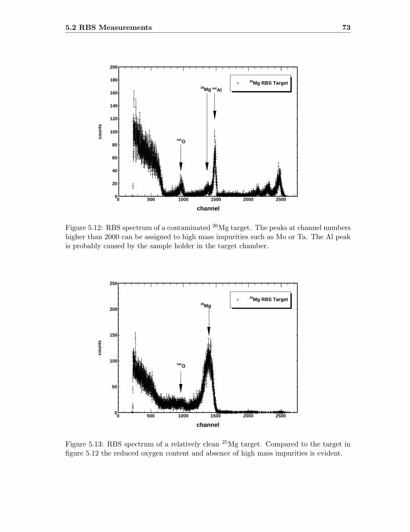
5.2 RBS Measurements 73
channel
0 500 1000 1500 2000 2500
cou
nts
0
20
40
60
80
100
120
140
160
180
200
Onat
Mg26Alnat
Mg RBS Target 26
Figure 5.12: RBS spectrum of a contaminated 26Mg target. The peaks at channel numbershigher than 2000 can be assigned to high mass impurities such as Mo or Ta. The Al peakis probably caused by the sample holder in the target chamber.
channel
0 500 1000 1500 2000 2500
cou
nts
0
50
100
150
200
250
Onat
Mg25Mg RBS Target 25
Figure 5.13: RBS spectrum of a relatively clean 25Mg target. Compared to the target infigure 5.12 the reduced oxygen content and absence of high mass impurities is evident.
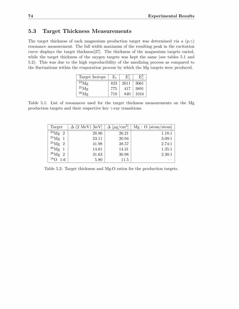
74 Experimental Results
5.3 Target Thickness Measurements
The target thickness of each magnesium production target was determined via a (p,γ)resonance measurement. The full width maximum of the resulting peak in the excitationcurve displays the target thickness[27]. The thickness of the magnesium targets varied,while the target thickness of the oxygen targets was kept the same (see tables 5.1 and5.2). This was due to the high reproducibility of the anodizing process as compared tothe fluctuations within the evaporation process by which the Mg targets were produced.
Target Isotope Er E1γ E2
γ24Mg 823 2611 306125Mg 775 417 389126Mg 718 840 1016
Table 5.1: List of resonances used for the target thickness measurements on the Mgproduction targets and their respective key γ-ray transitions.
Target ∆ (2 MeV) [keV] ∆ [µg/cm2] Mg : O [atom/atom]24Mg 2 28.86 26.21 1.18:125Mg 1 23.11 20.94 3.09:125Mg 2 41.98 38.57 2.74:126Mg 1 14.61 14.31 1.35:126Mg 2 31.63 30.98 2.30:118O 1-6 5.80 11.5 —
Table 5.2: Target thickness and Mg:O ratios for the production targets.

5.4 Background Correction Techniques 75
5.4 Background Correction Techniques
An intrinsic feature of detection systems based on neutron moderation and counting is theloss of energy information. As the neutrons are detected, one is not able to assign eachneutron to a specific reaction. Possible contamination of the targets leads to backgroundreactions influencing the experimental data. Especially if one compares the cross sectionsof the background reactions and reactions of interest it becomes evident that often evensmallest impurities can lead to problems during the data analysis (see figure 5.14). Here,with the Mg targets already contaminated with oxygen and the occurrence of carbon inalmost any material, there is no doubt of the occurence of background reactions such as13C(α,n)16O, 17O(α,n)20Ne and 18O(α,n)21Ne.It has to be noted that not only contamination within the targets but also e.g. on thebeamline slits can lead to an increase in background reactions. This was illustrated bysimply increasing the beam current on the beamline slits and recording the neutron yieldat a fixed energy. As a consequence, the current on the beamline slits was kept below 0.5µA.As shown in figure 5.15, the raw experimental data already allowed to identify mostresonance peaks and to assign them to specific background reactions. Two techniqueswere employed to correct the experimental data.
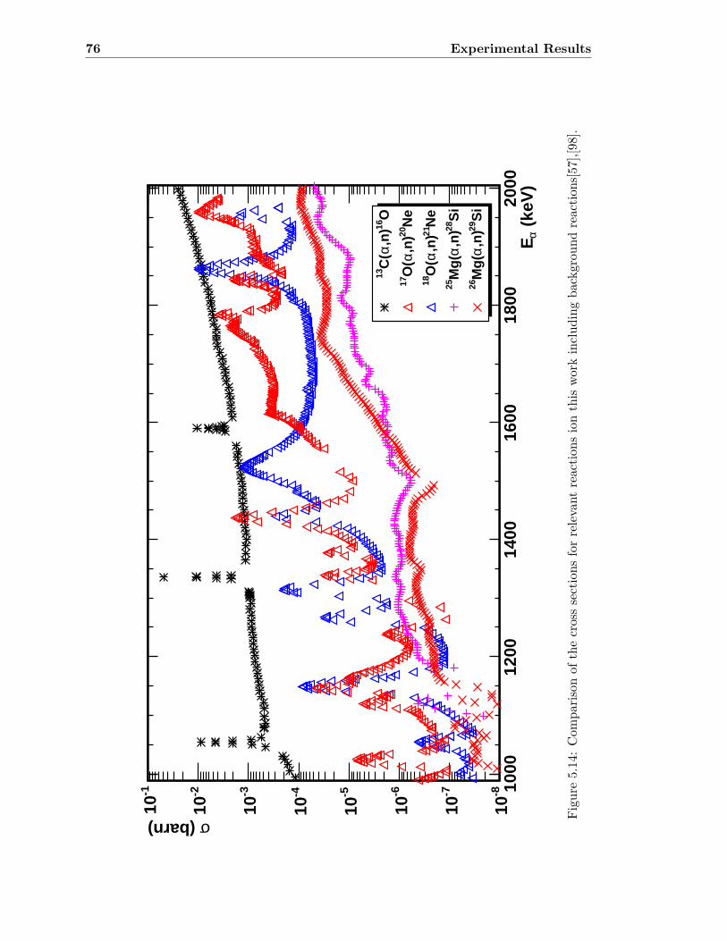
76 Experimental Results
(ke
V)
aE
1000
1200
1400
1600
1800
2000
(barn) s
-810
-710
-610
-510
-410
-310
-210
-110
O16
,n)
aC
(13
Ne
20,n
)a
O(
17
Ne
21,n
)a
O(
18
Si
28,n
)a
Mg(
25
Si
29,n
)a
Mg(
26
Figure
5.14:Com
parison
ofthecrosssectionsforrelevantreactionsionthis
work
includingbackgrou
ndreactions[57],[98].
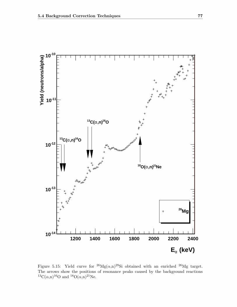
5.4 Background Correction Techniques 77
(keV)aE
1200 1400 1600 1800 2000 2200 2400
Yie
ld (
neut
rons
/alp
ha)
-1410
-1310
-1210
-1110
-1010
Mg26
O16,n)aC(13
O16,n)aC(13
Ne21,n)aO(18
Figure 5.15: Yield curve for 26Mg(α,n)29Si obtained with an enriched 26Mg target.The arrows show the positions of resonance peaks caused by the background reactions13C(α,n)16O and 18O(α,n)21Ne.
78 Experimental Results
5.4.1 Background Targets
The first technique involved the production of background targets. A background targetwas produced in the same way as a production target, but consisting of ”impurities” only.For the Mg production targets an isotopically enriched (99.75 %) 24Mg target served as anbackground target. This was possible since the 24Mg(α,n)27Si reaction occurs only at en-ergies outside the experimental energy range (Ethres = 8396 keV). For the 18O productiontargets a baked Ta backing was used as a background target.
18O background target
The measurements for the 18O background target showed only the 13C(α,n)16O reactionas an additional contribution to the experimental data (see figures 5.16 and 5.17). The13C(α,n)16O reaction, in general, was identified via the 13C(α,n)16O resonance peak at Er
= 1053 keV.A ROOT analysis code was developed executing the following steps :
• Identify peak position of Er = 1053 keV of 13C(α,n)16O reaction.
The peak positions of the 13C(α,n)16O reaction and the production target variedfor different targets. This is mainly due to the fact, that the contamination may besituated at different geometrical locations.
• Scale peak height of Eα = 1053 keV peak
Thickness and the level of the contamination directly influence the peak height inthe experimental data. Therefore, a scaling routine was implemented to match thecontamination levels.
• Match energy of background and production data
The energies at which background and production data are measured do not matchexactly. A routine was implemented to evaluate the background data at any givenenergy based on the experimental background data.
• Subtract evaluated background data from experimental data
Once background yield and energy binning are matched, the evaluated yield wassubtracted from the production data.
This routine was used for the directly recorded neutron yield Yr (which is already correctedfor dead time effects and cosmic background radiation).In figure 5.18 an example is shown, in which the uncorrected data, the evaluated back-ground target data and the corrected data are shown. It is evident that each target showsa noticeable, but different level of 13C contamination, despite identical target productionprocess and handling. The 13C contamination only had a noticeable effect on the ex-perimental data at energies below Eα = 1400 keV. The peak width of the 13C(α,n)16Oresonance peak also indicates a relatively thin target contamination.
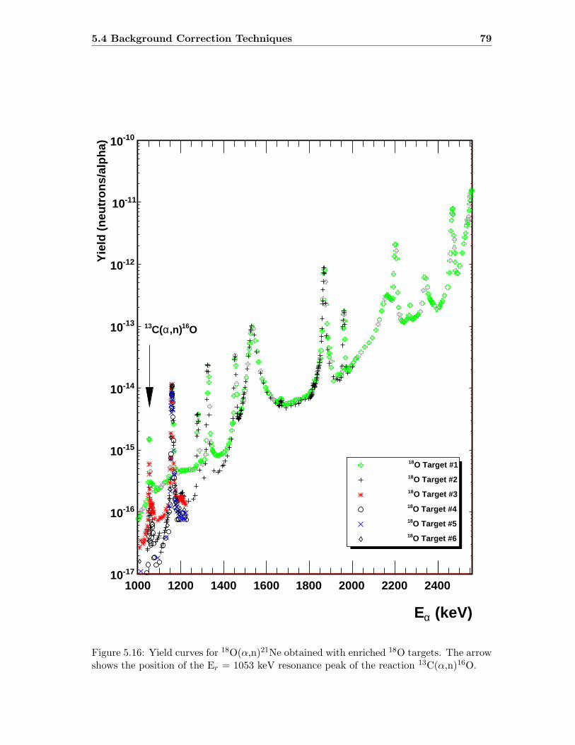
5.4 Background Correction Techniques 79
(keV)aE
1000 1200 1400 1600 1800 2000 2200 2400
Yie
ld (
neut
rons
/alp
ha)
-1710
-1610
-1510
-1410
-1310
-1210
-1110
-1010
O16,n)aC(13
O Target #118
O Target #218
O Target #318
O Target #418
O Target #518
O Target #618
Figure 5.16: Yield curves for 18O(α,n)21Ne obtained with enriched 18O targets. The arrowshows the position of the Er = 1053 keV resonance peak of the reaction 13C(α,n)16O.
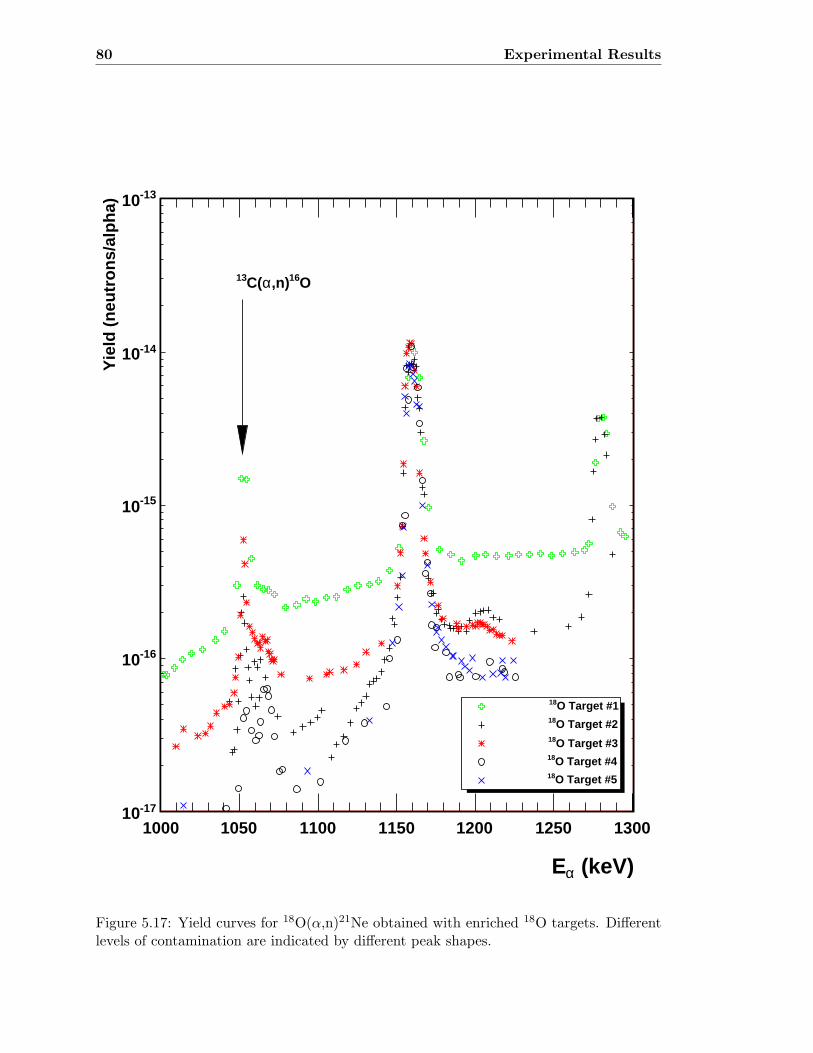
80 Experimental Results
(keV)aE
1000 1050 1100 1150 1200 1250 1300
Yie
ld (
neut
rons
/alp
ha)
-1710
-1610
-1510
-1410
-1310
O16,n)aC(13
O Target #118
O Target #218
O Target #318
O Target #418
O Target #518
Figure 5.17: Yield curves for 18O(α,n)21Ne obtained with enriched 18O targets. Differentlevels of contamination are indicated by different peak shapes.
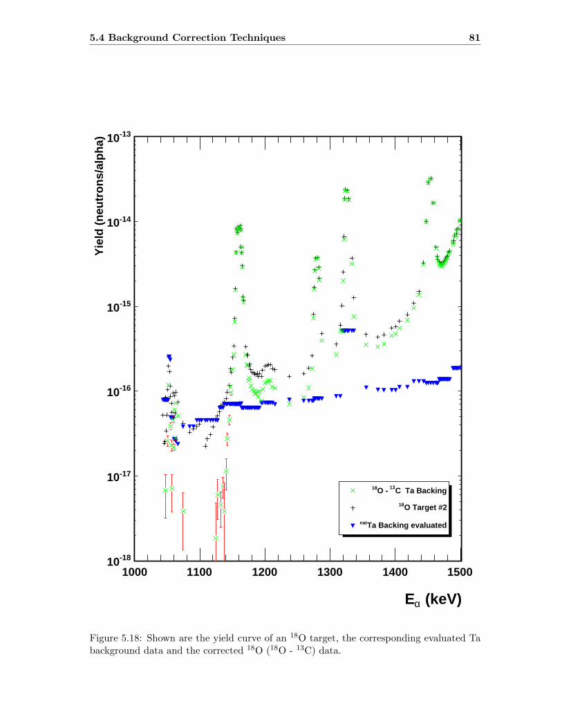
5.4 Background Correction Techniques 81
(keV)aE
1000 1100 1200 1300 1400 1500
Yie
ld (
neut
rons
/alp
ha)
-1810
-1710
-1610
-1510
-1410
-1310
C Ta Backing13O - 18
O Target #218
Ta Backing evaluatednat
Figure 5.18: Shown are the yield curve of an 18O target, the corresponding evaluated Tabackground data and the corrected 18O (18O - 13C) data.
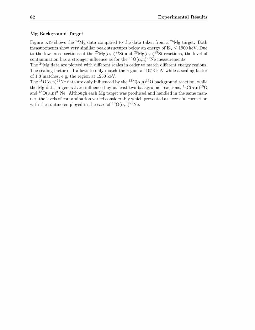
82 Experimental Results
Mg Background Target
Figure 5.19 shows the 24Mg data compared to the data taken from a 25Mg target. Bothmeasurements show very similiar peak structures below an energy of Eα ≤ 1900 keV. Dueto the low cross sections of the 25Mg(α,n)28Si and 26Mg(α,n)29Si reactions, the level ofcontamination has a stronger influence as for the 18O(α,n)21Ne measurements.The 24Mg data are plotted with different scales in order to match different energy regions.The scaling factor of 1 allows to only match the region at 1053 keV while a scaling factorof 1.3 matches, e.g, the region at 1230 keV.The 18O(α,n)21Ne data are only influenced by the 13C(α,n)16O background reaction, whilethe Mg data in general are influenced by at least two background reactions, 13C(α,n)16Oand 18O(α,n)21Ne. Although each Mg target was produced and handled in the same man-ner, the levels of contamination varied considerably which prevented a successful correctionwith the routine employed in the case of 18O(α,n)21Ne.
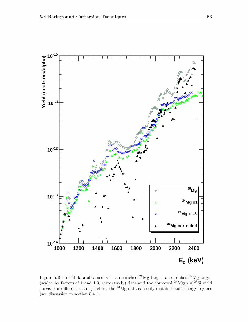
5.4 Background Correction Techniques 83
(keV)aE
1000 1200 1400 1600 1800 2000 2200 2400
Yie
ld (
neut
rons
/alp
ha)
-1410
-1310
-1210
-1110
-1010
Mg25
Mg x124
Mg x1.324
Mg corrected25
Figure 5.19: Yield data obtained with an enriched 25Mg target, an enriched 24Mg target(scaled by factors of 1 and 1.3, respectively) data and the corrected 25Mg(α,n)28Si yieldcurve. For different scaling factors, the 24Mg data can only match certain energy regions(see discussion in section 5.4.1).
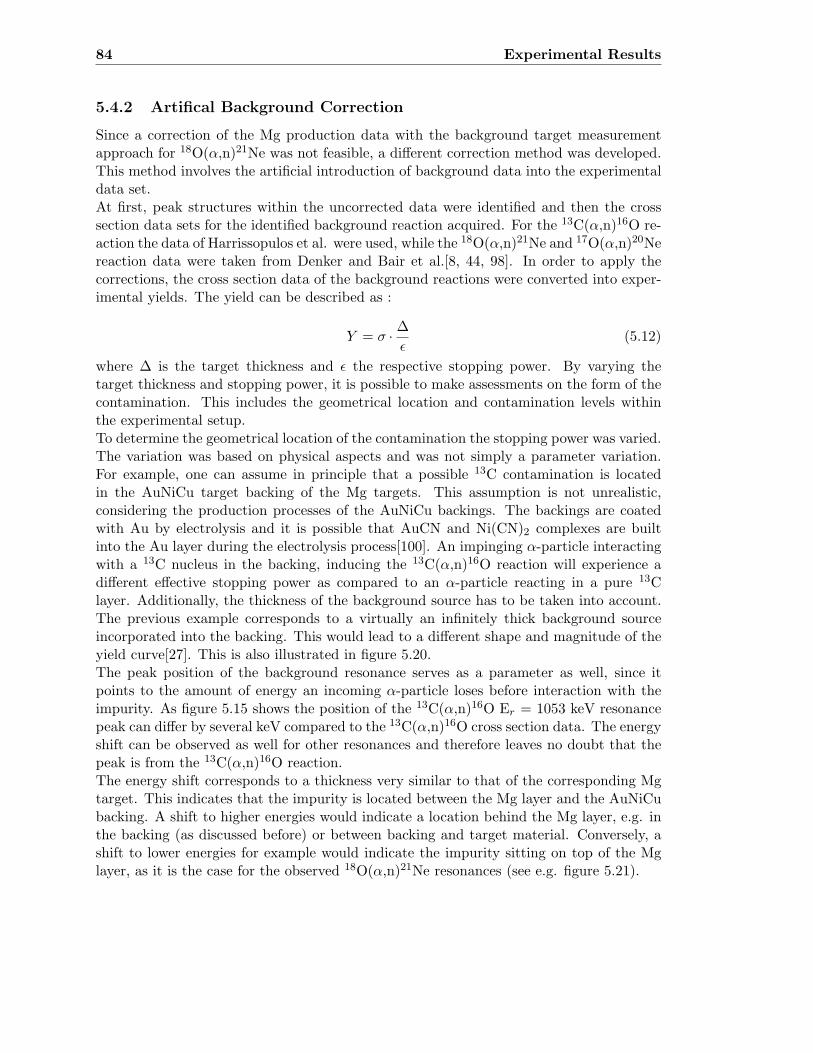
84 Experimental Results
5.4.2 Artifical Background Correction
Since a correction of the Mg production data with the background target measurementapproach for 18O(α,n)21Ne was not feasible, a different correction method was developed.This method involves the artificial introduction of background data into the experimentaldata set.At first, peak structures within the uncorrected data were identified and then the crosssection data sets for the identified background reaction acquired. For the 13C(α,n)16O re-action the data of Harrissopulos et al. were used, while the 18O(α,n)21Ne and 17O(α,n)20Nereaction data were taken from Denker and Bair et al.[8, 44, 98]. In order to apply thecorrections, the cross section data of the background reactions were converted into exper-imental yields. The yield can be described as :
Y = σ · ∆ϵ
(5.12)
where ∆ is the target thickness and ϵ the respective stopping power. By varying thetarget thickness and stopping power, it is possible to make assessments on the form of thecontamination. This includes the geometrical location and contamination levels withinthe experimental setup.To determine the geometrical location of the contamination the stopping power was varied.The variation was based on physical aspects and was not simply a parameter variation.For example, one can assume in principle that a possible 13C contamination is locatedin the AuNiCu target backing of the Mg targets. This assumption is not unrealistic,considering the production processes of the AuNiCu backings. The backings are coatedwith Au by electrolysis and it is possible that AuCN and Ni(CN)2 complexes are builtinto the Au layer during the electrolysis process[100]. An impinging α-particle interactingwith a 13C nucleus in the backing, inducing the 13C(α,n)16O reaction will experience adifferent effective stopping power as compared to an α-particle reacting in a pure 13Clayer. Additionally, the thickness of the background source has to be taken into account.The previous example corresponds to a virtually an infinitely thick background sourceincorporated into the backing. This would lead to a different shape and magnitude of theyield curve[27]. This is also illustrated in figure 5.20.The peak position of the background resonance serves as a parameter as well, since itpoints to the amount of energy an incoming α-particle loses before interaction with theimpurity. As figure 5.15 shows the position of the 13C(α,n)16O Er = 1053 keV resonancepeak can differ by several keV compared to the 13C(α,n)16O cross section data. The energyshift can be observed as well for other resonances and therefore leaves no doubt that thepeak is from the 13C(α,n)16O reaction.The energy shift corresponds to a thickness very similar to that of the corresponding Mgtarget. This indicates that the impurity is located between the Mg layer and the AuNiCubacking. A shift to higher energies would indicate a location behind the Mg layer, e.g. inthe backing (as discussed before) or between backing and target material. Conversely, ashift to lower energies for example would indicate the impurity sitting on top of the Mglayer, as it is the case for the observed 18O(α,n)21Ne resonances (see e.g. figure 5.21).

5.4 Background Correction Techniques 85
(keV)aE
1200 1400 1600 1800 2000 2200
Yie
ld (
neut
rons
/alp
ha)
-1610
-1510
-1410
-1310
-1210
-1110
-1010
C (AuNiCu)13
C (Mg)13
C thick component13
Figure 5.20: This plot illustrates the behaviour and magnitude for different types of 13Cimpurities. If the 13C is incorporated throughout the AuNiCu backing, the experimentaldata are influenced as displayed through the 13C thick component curve. 13C (AuNiCu)illustrates a thin impurity within the AuNiCu backing, while 13C (Mg) displays the 13Cbackground component for a thin impurity in the Mg layer.

86 Experimental Results
Mg CC AuNiCu
α
ε(Mg) ε(AuNiCu)ε(C) ε(C)
δE(+)δE(-)
Figure 5.21: Schematic drawing of a Mg target. As an example two different C components,at different locations, within a target are shown. δE(+) and δE(-) stand for an energy shiftto higher, respectively lower energy, while ϵ is the respective stopping power experienced bythe impinging α-particle. The widths of the layers do not correspond to actual proportions.
In summary the method involves the following steps :
• Identify background reactions
If possible, assign peak structures to know resonances of possible background reac-tions
• Calculate reaction yield for identified background reactions
Cross section data reported in the literature are converted into reaction yield data,taking into account parameters such as efficiency, enrichment etc.
• Determine possible physical location of impurity
Based on physical meaningful assumptions, vary stopping power and target thicknessof possible background reactions to match actual experimental data.
• Implement energy shift
Adjust the background reaction yield in energy and assign shifts according to locationof impurity.
• Match data and correct
Evaluate calculated reaction yield at energies given by experimental measurement.Correct experimental data by subtracting background reaction yield.
For each production target different levels and locations of contaminations were identified.Additionally, the number of contributing contaminations was determined. For example,
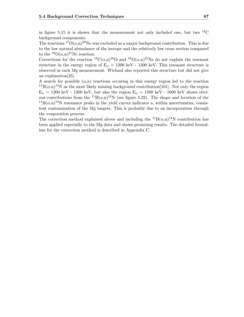
5.4 Background Correction Techniques 87
in figure 5.15 it is shown that the measurement not only included one, but two 13Cbackground components.The reactions 17O(α,n)20Ne was excluded as a major background contribution. This is dueto the low natural abundance of the isotope and the relatively low cross section comparedto the 18O(α,n)21Ne reaction.Corrections for the reaction 13C(α,n)16O and 18O(α,n)21Ne do not explain the resonantstructure in the energy region of Eα = 1200 keV - 1300 keV. This resonant structure isobserved in each Mg measurement. Wieland also reported this structure but did not givean explanation[45].A search for possible (α,n) reactions occuring in this energy region led to the reaction11B(α,n)14N as the most likely missing background contribution[101]. Not only the regionEα = 1200 keV - 1300 keV, but also the region Eα = 1500 keV - 1600 keV shows obvi-ous contributions from the 11B(α,n)14N (see figure 5.22). The shape and location of the11B(α,n)14N resonance peaks in the yield curves indicates a, within uncertainties, consis-tent contamination of the Mg targets. This is probably due to an incorporation throughthe evaporation process.The correction method explained above and including the 11B(α,n)14N contribution hasbeen applied especially to the Mg data and shows promising results. The detailed formal-ism for the correction method is described in Appendix C.

88 Experimental Results
(keV)aE
1200 1400 1600 1800 2000 2200 2400
Yie
ld (
neut
rons
/alp
ha)
-1410
-1310
-1210
-1110
-1010
Mg26
N scaled14,n)aB(11
Figure 5.22: Yield data of a 26Mg(α,n)29Si measurement and the cross section for thereaction 11B(α,n)14N[101]. The cross section is scaled to emphasize the correlation betweenboth data sets.

5.4 Background Correction Techniques 89
(keV)aE
1000 1200 1400 1600 1800 2000
Yie
ld (
neut
rons
/alp
ha)
-1610
-1510
-1410
-1310
-1210
-1110
Mg uncorrected26
B component11
Figure 5.23: Yield curve of a 26Mg(α,n)29Si measurement and the calculated backgrounddata for the 11B(α,n)14N component. The 11B(α,n)14N component is based on the crosssection provided by Wang et al. and, in contrast to figure 5.22, is additionally matchedfor thickness, stopping power etc. [101].

90 Experimental Results
5.5 25Mg(α,n)28Si
The experimental data on 25Mg(α,n)28Si showed two 13C, one 18O and one 11B backgroundcomponent. Below Eα = 1800 keV, the background does not allow a distinction betweenneutrons resulting from 25Mg(α,n)28Si or from one of the background reactions. As aconsequence, upper limits only were calculated for this energy region (see figure 5.24).For Eα ≥ 1800 keV the experimental data clearly show resonant structures from whichonly the region around Eα = 1866 keV had to be excluded due to the observation of the18O(α,n)21Ne(Er= 1866 keV) resonance. The resonances and their according resonanceparameters (resonance strength ωγ, total width Γ and resonance energy Er) were fittedand calculated. In table 5.4 they are listed and compared to the data reported by Wieland.The ambiguities in the Wieland data, such as a missing information on the backgroundtreatment, do not allow a quanititative comparison. Only the resonances at Er = 1834,2106, 2244 and 2338 keV could be confirmed in this work. An additional validation isgiven by the review of reported excited states (Ex) in the corresponding Nuclear DataSheets (see table 5.3) [102, 103].The derived resonance parameters and cross sections lead to an astrophysical S-factorwhich is up to an order of magnitude lower than the one reported by Wieland (see figure5.26). In particular the calculated resonance strengths differ substantially (see table 5.4).This should have an immediate impact on the reaction rate.
States of 29Si This work Wieland NDS
Eα Ecm Ex
2338 2015 13142 X X2244 1934 13061 X X2106 1816 12942 X X X2069 1783 12910 X2035 1754 12881 X1967 1695 12822 X1944 1676 12802 X1834 1581 12707 X X1818 1567 12693 X X1784 1537 12665 X
Table 5.3: List of resolved resonance states for 25Mg(α,n)28Si, compared to the work ofWieland and others (NDS) [45, 103]. Note, that the resonances at Eα = 1967, 1944, 1834,1818 overlap within errors (see also table 5.4).

5.5 25Mg(α,n)28Si 91
This
work
[keV]
Wieland
[keV]
Eα
Ecm
Ex
Γcm
ωγcm
Eα
Ecm
Ex
Γcm
ωγcm
2338
±3
2015
13412
81.20±
2.74
9.48E-04±
2.29E-05
2334±
10
2012
13139
20±
425±
42244
±2
1934
13061
66.84±
7.83
6.80E-04±
7.00E-06
2245±
51935
13062
20±
520±
22106
±3
1816
12942
108.19
±3.5
3.80E-04±
1.04E-05
2116±
10
1824
12951
2069±
51784
12910
2035
±2
1754
12880
44.37±
1.31
1.49E-04±
3.13E-06
2006±
15
1729
12856
8±
32.6
±0.8
1967
±2
1695
12822
86.24±
1.26
1.31E-04±
1.55E-06
1944±
15
1676
12802
4±
20.93±
0.4
1896±
15
1634
12761
22±
10
0.42±
0.2
1834
±3
1581
12707
21.97±
3.87
1.30E-05±
1.00E-06
1837±
20
1584
12710
5±
20.27±
0.17
1818
±4
1567
12693
96.55±
3.42
3.28E-05±
1.30E-06
1784±
71538
12664
5±3
0.25±
0.18
Tab
le5.4:
25Mg(α,n)2
8Siresonan
ceparametersfrom
Wielandcomparedto
theparametersobtained
inthis
work[45].
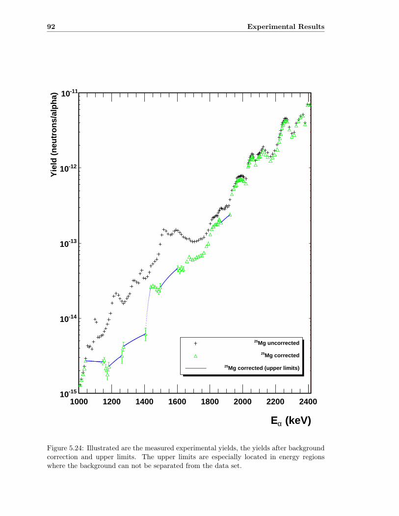
92 Experimental Results
(keV)aE
1000 1200 1400 1600 1800 2000 2200 2400
Yie
ld (
neut
rons
/alp
ha)
-1510
-1410
-1310
-1210
-1110
Mg uncorrected25
Mg corrected25
Mg corrected (upper limits)25
Figure 5.24: Illustrated are the measured experimental yields, the yields after backgroundcorrection and upper limits. The upper limits are especially located in energy regionswhere the background can not be separated from the data set.
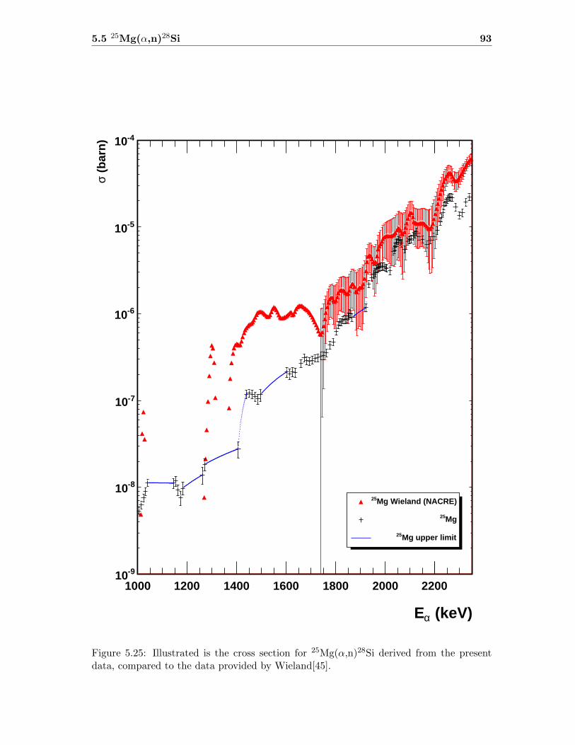
5.5 25Mg(α,n)28Si 93
(keV)aE
1000 1200 1400 1600 1800 2000 2200
(ba
rn)
s
-910
-810
-710
-610
-510
-410
Mg Wieland (NACRE)25
Mg25
Mg upper limit25
Figure 5.25: Illustrated is the cross section for 25Mg(α,n)28Si derived from the presentdata, compared to the data provided by Wieland[45].
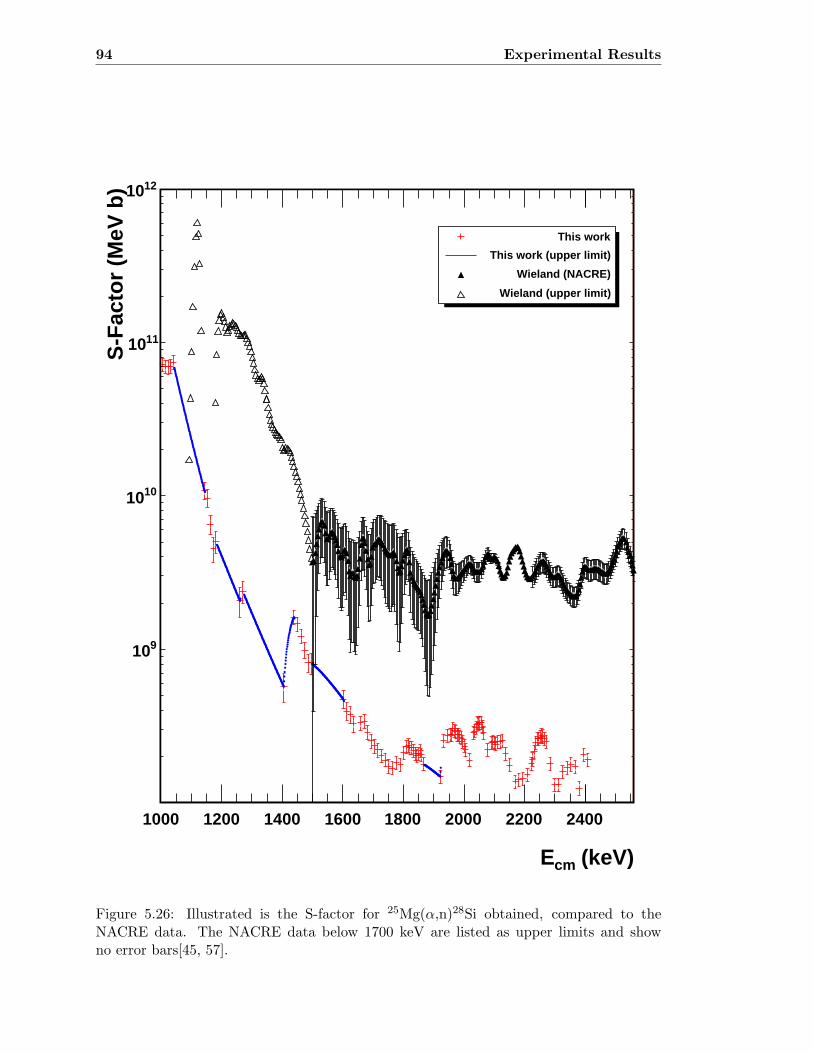
94 Experimental Results
(keV)cmE
1000 1200 1400 1600 1800 2000 2200 2400
S-F
acto
r (M
eV b
)
910
1010
1110
1210
This work
This work (upper limit)
Wieland (NACRE)
Wieland (upper limit)
Figure 5.26: Illustrated is the S-factor for 25Mg(α,n)28Si obtained, compared to theNACRE data. The NACRE data below 1700 keV are listed as upper limits and showno error bars[45, 57].
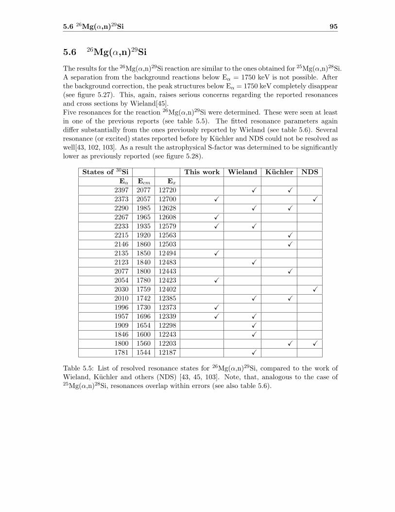
5.6 26Mg(α,n)29Si 95
5.6 26Mg(α,n)29Si
The results for the 26Mg(α,n)29Si reaction are similar to the ones obtained for 25Mg(α,n)28Si.A separation from the background reactions below Eα = 1750 keV is not possible. Afterthe background correction, the peak structures below Eα = 1750 keV completely disappear(see figure 5.27). This, again, raises serious concerns regarding the reported resonancesand cross sections by Wieland[45].Five resonances for the reaction 26Mg(α,n)29Si were determined. These were seen at leastin one of the previous reports (see table 5.5). The fitted resonance parameters againdiffer substantially from the ones previously reported by Wieland (see table 5.6). Severalresonance (or excited) states reported before by Kuchler and NDS could not be resolved aswell[43, 102, 103]. As a result the astrophysical S-factor was determined to be significantlylower as previously reported (see figure 5.28).
States of 30Si This work Wieland Kuchler NDS
Eα Ecm Ex
2397 2077 12720 X X2373 2057 12700 X X2290 1985 12628 X X2267 1965 12608 X2233 1935 12579 X X2215 1920 12563 X2146 1860 12503 X2135 1850 12494 X2123 1840 12483 X2077 1800 12443 X2054 1780 12423 X2030 1759 12402 X2010 1742 12385 X X1996 1730 12373 X1957 1696 12339 X X1909 1654 12298 X1846 1600 12243 X1800 1560 12203 X X1781 1544 12187 X
Table 5.5: List of resolved resonance states for 26Mg(α,n)29Si, compared to the work ofWieland, Kuchler and others (NDS) [43, 45, 103]. Note, that, analogous to the case of25Mg(α,n)28Si, resonances overlap within errors (see also table 5.6).
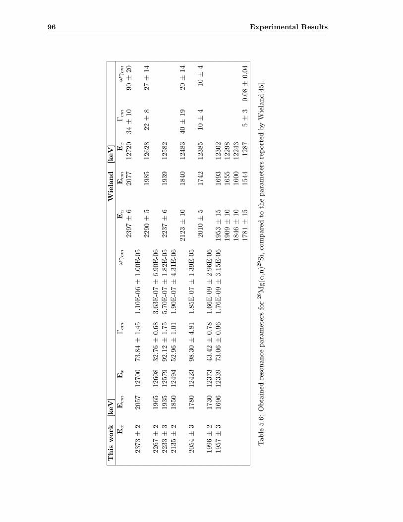
96 Experimental Results
This
work
[keV]
Wieland
[keV]
Eα
Ecm
Ex
Γcm
ωγcm
Eα
Ecm
Ex
Γcm
ωγcm
2397±
6207
712
720
34±
1090±
202373
±2
2057
12700
73.84±
1.45
1.10E-06±
1.00E-05
2290±
5198
512
628
22±
827±
142267
±2
1965
12608
32.76±
0.68
3.63E-07±
6.90E-06
2233
±3
1935
12579
92.12±
1.75
5.70E-07±
1.82E-05
2237±
619
39125
822135
±2
1850
12494
52.96±
1.01
1.90E-07±
4.31E-06
2123±
10
184
012
483
40±
1920±
142054
±3
1780
12423
98.30±
4.81
1.85E-07±
1.39E-05
2010±
5174
212
385
10±
410
±4
1996
±2
1730
12373
43.42±
0.78
1.66E-09±
2.96E-06
1957
±3
1696
12339
73.06±
0.96
1.76E-09±
3.15E-06
1953±
15
1693
123
021909±
10
165
512
298
1846±
10
160
012
243
1781±
15
154
412
875±
30.08±
0.04
Tab
le5.6:
Obtained
resonan
ceparam
etersfor26Mg(α,n)2
9Si,comparedto
theparametersreported
byW
ieland[45].

5.6 26Mg(α,n)29Si 97
(keV)aE
1000 1200 1400 1600 1800 2000 2200
(ba
rn)
s
-1010
-910
-810
-710
-610
-510
-410
-310
Mg Wieland (NACRE)26
Mg26
Mg upper limit26
Figure 5.27: Shown are the cross sections for 26Mg(α,n)29Si obtained in this work, com-pared to the cross section data reported by NACRE. It has to be noted, that the NACREdata are dominated by the data achieved of Wieland[45, 57]. Below 1700 keV they arelisted as upper limits and show no error bars.
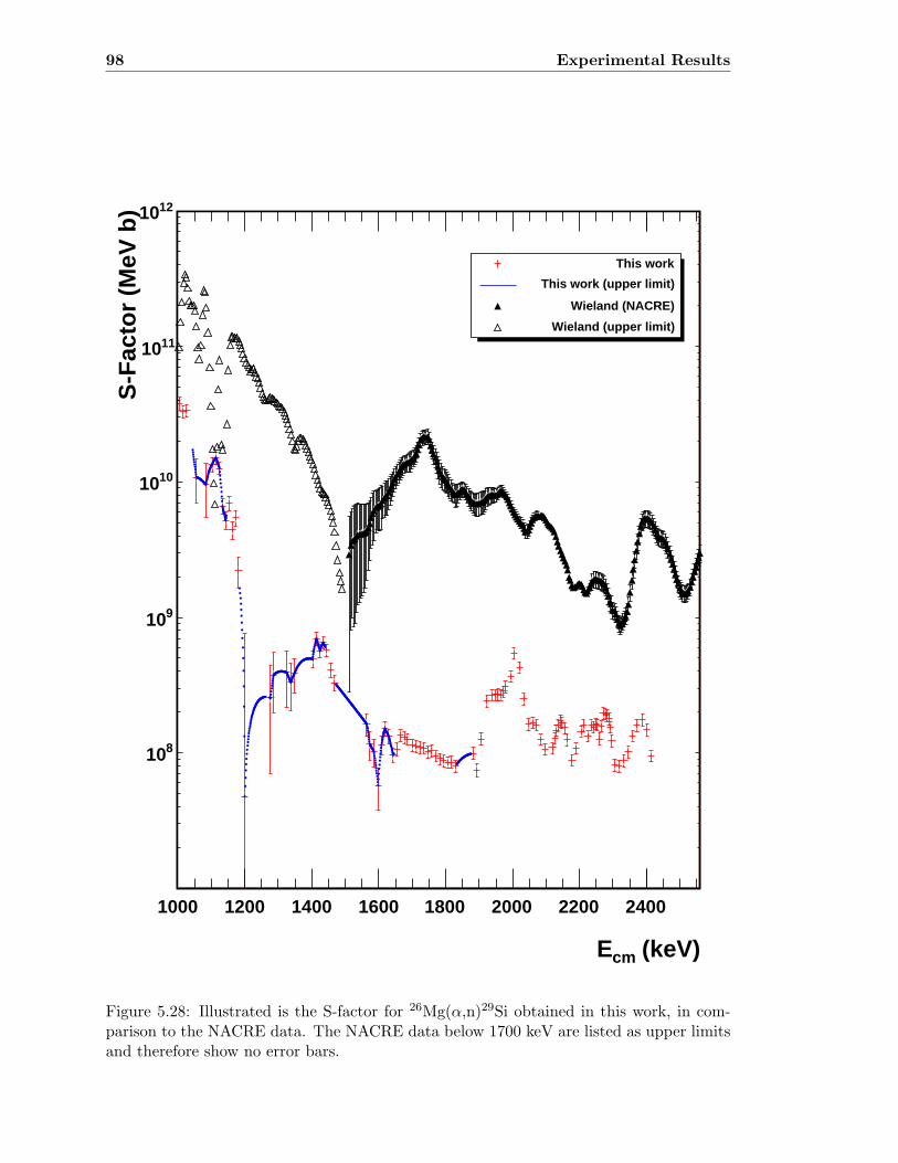
98 Experimental Results
(keV)cmE
1000 1200 1400 1600 1800 2000 2200 2400
S-F
acto
r (M
eV b
)
810
910
1010
1110
1210
This work
This work (upper limit)
Wieland (NACRE)
Wieland (upper limit)
Figure 5.28: Illustrated is the S-factor for 26Mg(α,n)29Si obtained in this work, in com-parison to the NACRE data. The NACRE data below 1700 keV are listed as upper limitsand therefore show no error bars.
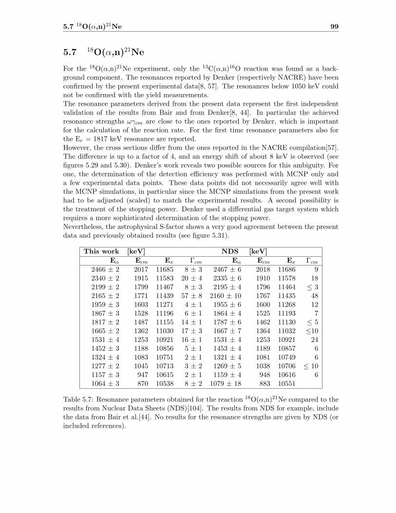
5.7 18O(α,n)21Ne 99
5.7 18O(α,n)21Ne
For the 18O(α,n)21Ne experiment, only the 13C(α,n)16O reaction was found as a back-ground component. The resonances reported by Denker (respectively NACRE) have beenconfirmed by the present experimental data[8, 57]. The resonances below 1050 keV couldnot be confirmed with the yield measurements.The resonance parameters derived from the present data represent the first independentvalidation of the results from Bair and from Denker[8, 44]. In particular the achievedresonance strengths ωγcm are close to the ones reported by Denker, which is importantfor the calculation of the reaction rate. For the first time resonance parameters also forthe Er = 1817 keV resonance are reported.However, the cross sections differ from the ones reported in the NACRE compilation[57].The difference is up to a factor of 4, and an energy shift of about 8 keV is observed (seefigures 5.29 and 5.30). Denker’s work reveals two possible sources for this ambiguity. Forone, the determination of the detection efficiency was performed with MCNP only anda few experimental data points. These data points did not necessarily agree well withthe MCNP simulations, in particular since the MCNP simulations from the present workhad to be adjusted (scaled) to match the experimental results. A second possibility isthe treatment of the stopping power. Denker used a differential gas target system whichrequires a more sophisticated determination of the stopping power.Nevertheless, the astrophysical S-factor shows a very good agreement between the presentdata and previously obtained results (see figure 5.31).
This work [keV] NDS [keV]
Eα Ecm Ex Γcm Eα Ecm Ex Γcm
2466 ± 2 2017 11685 8 ± 3 2467 ± 6 2018 11686 92340 ± 2 1915 11583 20 ± 4 2335 ± 6 1910 11578 182199 ± 2 1799 11467 8 ± 3 2195 ± 4 1796 11464 ≤ 32165 ± 2 1771 11439 57 ± 8 2160 ± 10 1767 11435 481959 ± 3 1603 11271 4 ± 1 1955 ± 6 1600 11268 121867 ± 3 1528 11196 6 ± 1 1864 ± 4 1525 11193 71817 ± 2 1487 11155 14 ± 1 1787 ± 6 1462 11130 ≤ 51665 ± 2 1362 11030 17 ± 3 1667 ± 7 1364 11032 ≤101531 ± 4 1253 10921 16 ± 1 1531 ± 4 1253 10921 241452 ± 3 1188 10856 5 ± 1 1453 ± 4 1189 10857 61324 ± 4 1083 10751 2 ± 1 1321 ± 4 1081 10749 61277 ± 2 1045 10713 3 ± 2 1269 ± 5 1038 10706 ≤ 101157 ± 3 947 10615 2 ± 1 1159 ± 4 948 10616 61064 ± 3 870 10538 8 ± 2 1079 ± 18 883 10551
Table 5.7: Resonance parameters obtained for the reaction 18O(α,n)21Ne compared to theresults from Nuclear Data Sheets (NDS)[104]. The results from NDS for example, includethe data from Bair et al.[44]. No results for the resonance strengths are given by NDS (orincluded references).
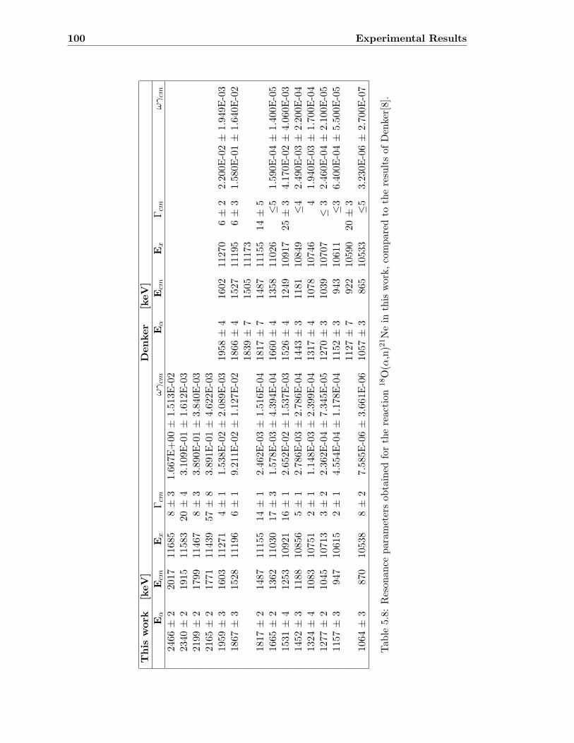
100 Experimental Results
This
work
[keV]
Denker
[keV]
Eα
Ecm
Ex
Γcm
ωγcm
Eα
Ecm
Ex
Γcm
ωγcm
2466
±2
2017
11685
8±
31.667E
+00
±1.51
3E-02
2340
±2
1915
11583
20±
43.109E
-01±
1.61
2E-03
2199
±2
1799
11467
8±
33.890E
-01±
3.84
0E-03
2165
±2
1771
11439
57±
83.891E
-01±
4.62
2E-03
1959
±3
1603
11271
4±
11.538E
-02±
2.08
9E-03
1958±
41602
1127
06±
22.200
E-02±
1.949
E-03
1867
±3
1528
11196
6±
19.211E
-02±
1.12
7E-02
1866±
41527
1119
56±
31.580
E-01±
1.640
E-02
1839±
71505
111
731817
±2
1487
11155
14±
12.462E
-03±
1.51
6E-04
1817±
71487
1115
514
±5
1665
±2
1362
11030
17±
31.578E
-03±
4.39
4E-04
1660±
41358
1102
6≤5
1.590
E-04±
1.400
E-05
1531
±4
1253
10921
16±
12.652E
-02±
1.53
7E-03
1526±
41249
1091
725
±3
4.170
E-02±
4.060
E-03
1452
±3
1188
10856
5±
12.786E
-03±
2.78
6E-04
1443±
31181
1084
9≤4
2.490
E-03±
2.200
E-04
1324
±4
1083
10751
2±
11.148E
-03±
2.39
9E-04
1317±
41078
1074
64
1.940
E-03±
1.700
E-04
1277
±2
1045
10713
3±
22.362E
-04±
7.34
5E-05
1270±
31039
1070
7≤
32.460
E-04±
2.100
E-05
1157
±3
947
10615
2±
14.554E
-04±
1.17
8E-04
1152±
3943
1061
1≤3
6.400
E-04±
5.500
E-05
1127±
7922
105
9020±
31064
±3
870
10538
8±
27.585E
-06±
3.66
1E-06
1057±
3865
1053
3≤5
3.230
E-06±
2.700
E-07
Tab
le5.8:
Reson
ance
param
etersob
tained
forthereaction
18O(α
,n)2
1Nein
this
work,comparedto
theresultsof
Denker[8].

5.7 18O(α,n)21Ne 101
(keV)aE
1000 1200 1400 1600 1800 2000 2200 2400
(ba
rn)
s
-810
-710
-610
-510
-410
-310
-210
-110
1
O NACRE x 1 18
This work
Figure 5.29: Illustrated is the cross section for 18O(α,n)21Ne, compared to the NACREdata, which includes the data obtained by Bair and those obtained by Denker[8, 44, 57].Note, that an energy shift and a scaling difference between both data sets exists.
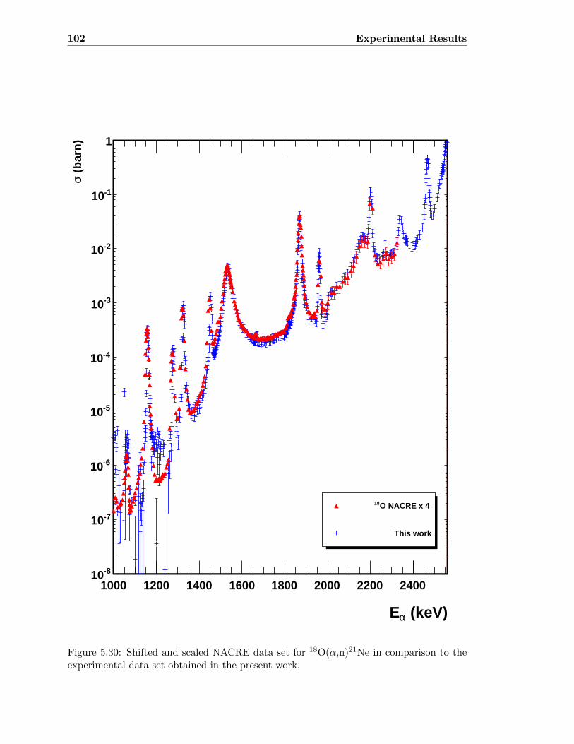
102 Experimental Results
(keV)aE
1000 1200 1400 1600 1800 2000 2200 2400
(ba
rn)
s
-810
-710
-610
-510
-410
-310
-210
-110
1
O NACRE x 4 18
This work
Figure 5.30: Shifted and scaled NACRE data set for 18O(α,n)21Ne in comparison to theexperimental data set obtained in the present work.
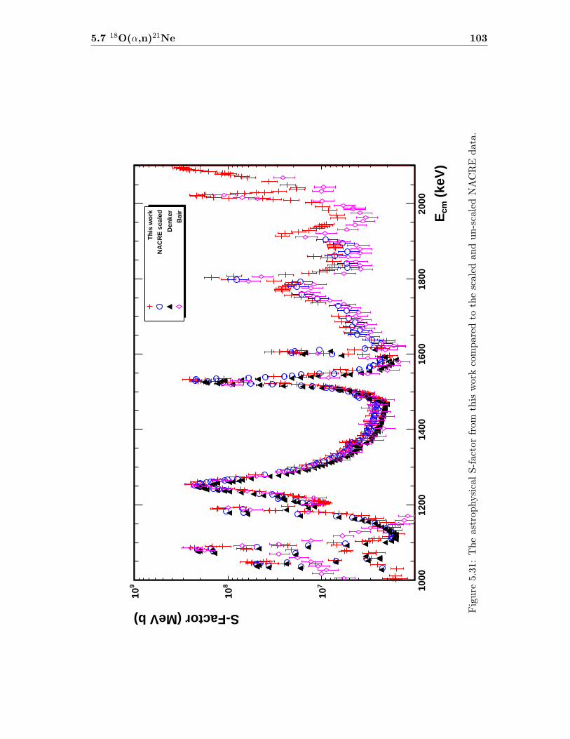
5.7 18O(α,n)21Ne 103
(ke
V)
cmE
1000
1200
1400
1600
1800
2000
S-Factor (MeV b)
710
810
910
Thi
s w
ork
NA
CR
E s
cale
d
Den
ker
Bai
r
Figure
5.31:Theastrop
hysicalS-factorfrom
this
work
comparedto
thescaledandun-scaledNACRE
data.
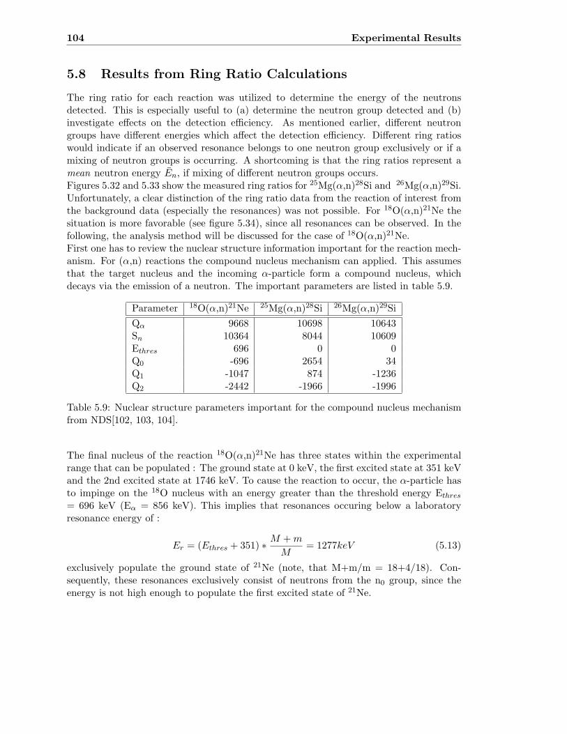
104 Experimental Results
5.8 Results from Ring Ratio Calculations
The ring ratio for each reaction was utilized to determine the energy of the neutronsdetected. This is especially useful to (a) determine the neutron group detected and (b)investigate effects on the detection efficiency. As mentioned earlier, different neutrongroups have different energies which affect the detection efficiency. Different ring ratioswould indicate if an observed resonance belongs to one neutron group exclusively or if amixing of neutron groups is occurring. A shortcoming is that the ring ratios represent amean neutron energy En, if mixing of different neutron groups occurs.Figures 5.32 and 5.33 show the measured ring ratios for 25Mg(α,n)28Si and 26Mg(α,n)29Si.Unfortunately, a clear distinction of the ring ratio data from the reaction of interest fromthe background data (especially the resonances) was not possible. For 18O(α,n)21Ne thesituation is more favorable (see figure 5.34), since all resonances can be observed. In thefollowing, the analysis method will be discussed for the case of 18O(α,n)21Ne.First one has to review the nuclear structure information important for the reaction mech-anism. For (α,n) reactions the compound nucleus mechanism can applied. This assumesthat the target nucleus and the incoming α-particle form a compound nucleus, whichdecays via the emission of a neutron. The important parameters are listed in table 5.9.
Parameter 18O(α,n)21Ne 25Mg(α,n)28Si 26Mg(α,n)29Si
Qα 9668 10698 10643Sn 10364 8044 10609Ethres 696 0 0Q0 -696 2654 34Q1 -1047 874 -1236Q2 -2442 -1966 -1996
Table 5.9: Nuclear structure parameters important for the compound nucleus mechanismfrom NDS[102, 103, 104].
The final nucleus of the reaction 18O(α,n)21Ne has three states within the experimentalrange that can be populated : The ground state at 0 keV, the first excited state at 351 keVand the 2nd excited state at 1746 keV. To cause the reaction to occur, the α-particle hasto impinge on the 18O nucleus with an energy greater than the threshold energy Ethres
= 696 keV (Eα = 856 keV). This implies that resonances occuring below a laboratoryresonance energy of :
Er = (Ethres + 351) ∗ M +m
M= 1277keV (5.13)
exclusively populate the ground state of 21Ne (note, that M+m/m = 18+4/18). Con-sequently, these resonances exclusively consist of neutrons from the n0 group, since theenergy is not high enough to populate the first excited state of 21Ne.
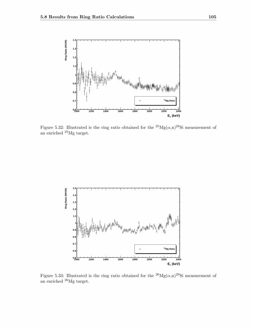
5.8 Results from Ring Ratio Calculations 105
(keV)aE1000 1200 1400 1600 1800 2000 2200 2400
Rin
g R
atio
(IR
/OR
)
0.6
0.7
0.8
0.9
1
1.1
1.2
1.3
1.4
Mg Ratio25
Figure 5.32: Illustrated is the ring ratio obtained for the 25Mg(α,n)28Si measurement ofan enriched 25Mg target.
(keV)aE1000 1200 1400 1600 1800 2000 2200 2400
Rin
g R
atio
(IR
/OR
)
0.5
0.6
0.7
0.8
0.9
1
1.1
1.2
1.3
1.4
1.5
Mg Ratio26
Figure 5.33: Illustrated is the ring ratio obtained for the 26Mg(α,n)29Si measurement ofan enriched 26Mg target.
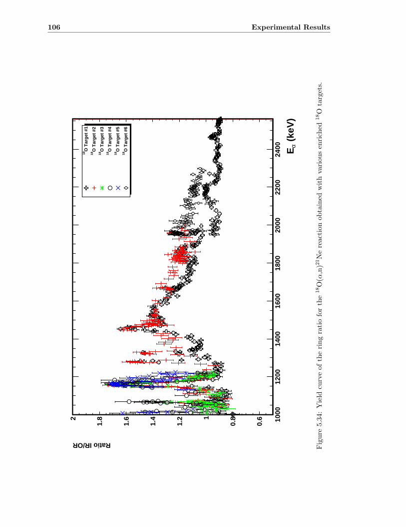
106 Experimental Results
(ke
V)
aE
1000
1200
1400
1600
1800
2000
2200
2400
Ratio IR/OR
0.6
0.81
1.2
1.4
1.6
1.82
O T
arg
et #
118
O T
arg
et #
218
O T
arg
et #
318
O T
arg
et #
418
O T
arg
et #
518
O T
arg
et #
618
Figure
5.34:Yield
curveof
theringratioforthe
18O(α
,n)2
1Nereactionobtained
withvariou
sen
riched
18O
targets.
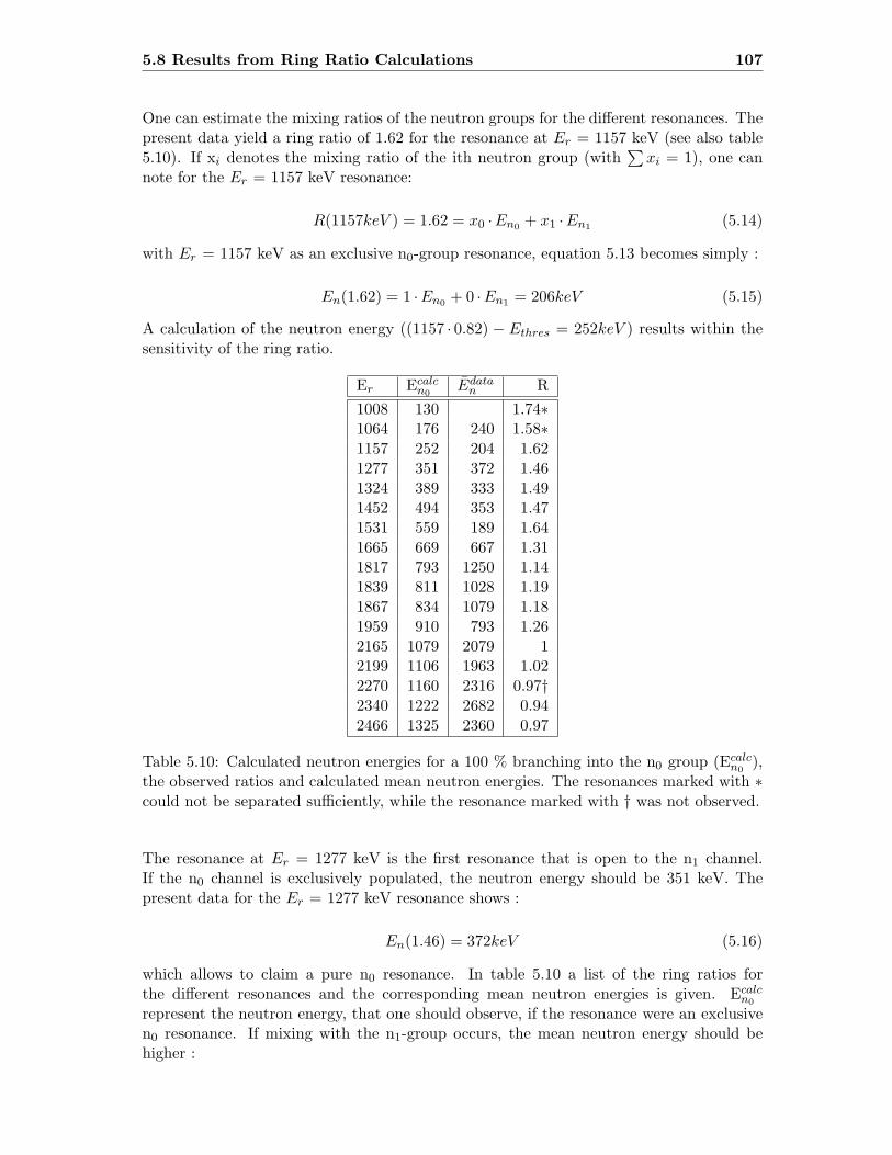
5.8 Results from Ring Ratio Calculations 107
One can estimate the mixing ratios of the neutron groups for the different resonances. Thepresent data yield a ring ratio of 1.62 for the resonance at Er = 1157 keV (see also table5.10). If xi denotes the mixing ratio of the ith neutron group (with
∑xi = 1), one can
note for the Er = 1157 keV resonance:
R(1157keV ) = 1.62 = x0 ·En0 + x1 ·En1 (5.14)
with Er = 1157 keV as an exclusive n0-group resonance, equation 5.13 becomes simply :
En(1.62) = 1 ·En0 + 0 ·En1 = 206keV (5.15)
A calculation of the neutron energy ((1157 · 0.82) − Ethres = 252keV ) results within thesensitivity of the ring ratio.
Er Ecalcn0
Edatan R
1008 130 1.74∗1064 176 240 1.58∗1157 252 204 1.621277 351 372 1.461324 389 333 1.491452 494 353 1.471531 559 189 1.641665 669 667 1.311817 793 1250 1.141839 811 1028 1.191867 834 1079 1.181959 910 793 1.262165 1079 2079 12199 1106 1963 1.022270 1160 2316 0.97†2340 1222 2682 0.942466 1325 2360 0.97
Table 5.10: Calculated neutron energies for a 100 % branching into the n0 group (Ecalcn0
),the observed ratios and calculated mean neutron energies. The resonances marked with ∗could not be separated sufficiently, while the resonance marked with † was not observed.
The resonance at Er = 1277 keV is the first resonance that is open to the n1 channel.If the n0 channel is exclusively populated, the neutron energy should be 351 keV. Thepresent data for the Er = 1277 keV resonance shows :
En(1.46) = 372keV (5.16)
which allows to claim a pure n0 resonance. In table 5.10 a list of the ring ratios forthe different resonances and the corresponding mean neutron energies is given. Ecalc
n0
represent the neutron energy, that one should observe, if the resonance were an exclusiven0 resonance. If mixing with the n1-group occurs, the mean neutron energy should behigher :
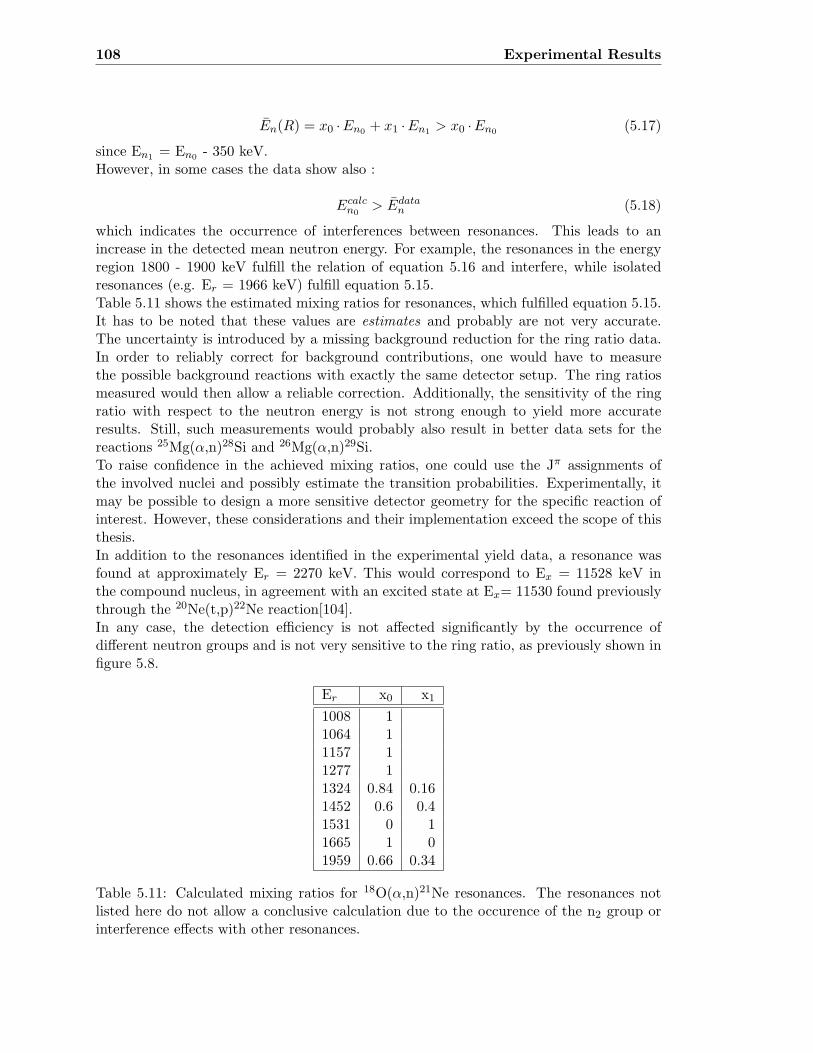
108 Experimental Results
En(R) = x0 ·En0 + x1 ·En1 > x0 ·En0 (5.17)
since En1 = En0 - 350 keV.However, in some cases the data show also :
Ecalcn0
> Edatan (5.18)
which indicates the occurrence of interferences between resonances. This leads to anincrease in the detected mean neutron energy. For example, the resonances in the energyregion 1800 - 1900 keV fulfill the relation of equation 5.16 and interfere, while isolatedresonances (e.g. Er = 1966 keV) fulfill equation 5.15.Table 5.11 shows the estimated mixing ratios for resonances, which fulfilled equation 5.15.It has to be noted that these values are estimates and probably are not very accurate.The uncertainty is introduced by a missing background reduction for the ring ratio data.In order to reliably correct for background contributions, one would have to measurethe possible background reactions with exactly the same detector setup. The ring ratiosmeasured would then allow a reliable correction. Additionally, the sensitivity of the ringratio with respect to the neutron energy is not strong enough to yield more accurateresults. Still, such measurements would probably also result in better data sets for thereactions 25Mg(α,n)28Si and 26Mg(α,n)29Si.To raise confidence in the achieved mixing ratios, one could use the Jπ assignments ofthe involved nuclei and possibly estimate the transition probabilities. Experimentally, itmay be possible to design a more sensitive detector geometry for the specific reaction ofinterest. However, these considerations and their implementation exceed the scope of thisthesis.In addition to the resonances identified in the experimental yield data, a resonance wasfound at approximately Er = 2270 keV. This would correspond to Ex = 11528 keV inthe compound nucleus, in agreement with an excited state at Ex= 11530 found previouslythrough the 20Ne(t,p)22Ne reaction[104].In any case, the detection efficiency is not affected significantly by the occurrence ofdifferent neutron groups and is not very sensitive to the ring ratio, as previously shown infigure 5.8.
Er x0 x1
1008 11064 11157 11277 11324 0.84 0.161452 0.6 0.41531 0 11665 1 01959 0.66 0.34
Table 5.11: Calculated mixing ratios for 18O(α,n)21Ne resonances. The resonances notlisted here do not allow a conclusive calculation due to the occurence of the n2 group orinterference effects with other resonances.
5.9 Reaction Rates 109
5.9 Reaction Rates
As already discussed in section 2.4, the reaction rate determines the outcome of the networkcalculations, which will lead to an impact assessment for stellar nucleosynthesis. Nuclearstructure effects and uncertainties in the experimental data entail the use of assumptionsfor the determination of the reaction rate.In general, the reaction rate is dependent on the reaction mechanism. For (α,n) reactionsthe mechanism involves the formation of a compound nucleus. As a consequence, the oc-currence of resonant behaviour is strongly favored, which results in a resonant componentof the reaction rate (see also 2.3):
⟨σv⟩r =(
2π
µkT
)3/2
~2∑i
(ωγ)iexp
(− Ei
kT
)f (5.19)
where i denotes the specific resonance observed. For 25Mg(α,n)28Si and 26Mg(α,n)29Sithis is the situation in the energy range Eα = 1800 keV. As illustrated previously, theexperimental data do not allow an accurate determination of the cross sections downto lower astrophysical energies, however. For these energy regions the cross section, orrespectively S-factor, was assumed to be constant at 1.36 · 108 MeVb for 25Mg(α,n)28Siand 7.97 · 108 MeVb for 26Mg(α,n)29Si. The corresponding reaction rate can then beexpressed as :
⟨σv⟩sfactor =(2
µ
)1/2 ∆
(kT )3/2S(E0)(1 +
5
12τ)exp (−τ) (5.20)
with ∆ as the effective width of the relevant energy window and τ being defined as :
τ =3E0
kT≫ 1 (5.21)
This constitutes then a second component for the reaction rate[27].For energy regions completely outside the experimental range investigated in this thesis,the cross section data sets were complemented. By data taken from the NACRE compi-lation the total reaction rate becomes therefore :
⟨σv⟩total = ⟨σv⟩r + ⟨σv⟩sfactor + ⟨σv⟩NACRE (5.22)
including the energy ranges and resonances not investigated in this thesis (⟨σv⟩NACRE)[27,57].Due to the substantial background corrections and resulting lower resonance strengths, thereaction rates for the reactions 25Mg(α,n)28Si and 26Mg(α,n)29Si obtained in this work areup to several orders of magnitude lower than those previously reported. This is illustratedin figures 5.35 and 5.36, where the different calculated components and the data fromliterature are shown. The differences between each component illustrate the importanceof accurate resonance information from experimental data sets.
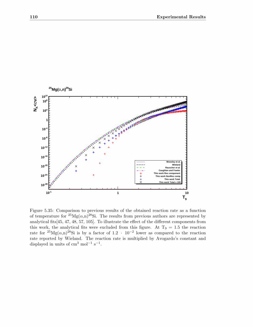
110 Experimental Results
9T-110 1 10
v>s<A
N
-2810
-2410
-2010
-1610
-1210
-810
-410
1
410
810
1010
Woosley et al.Wieland
Rauscher et al.Caughlan and Fowler
This work Res componentThis work NonRes comp
This work Total This work Total x 100
Si29,n)aMg(25
Figure 5.35: Comparison to previous results of the obtained reaction rate as a functionof temperature for 25Mg(α,n)28Si. The results from previous authors are represented byanalytical fits[45, 47, 48, 57, 105]. To illustrate the effect of the different components fromthis work, the analytical fits were excluded from this figure. At T9 = 1.5 the reactionrate for 25Mg(α,n)28Si is by a factor of 1.2 · 10−2 lower as compared to the reactionrate reported by Wieland. The reaction rate is multiplied by Avogardo’s constant anddisplayed in units of cm3 mol−1 s−1.
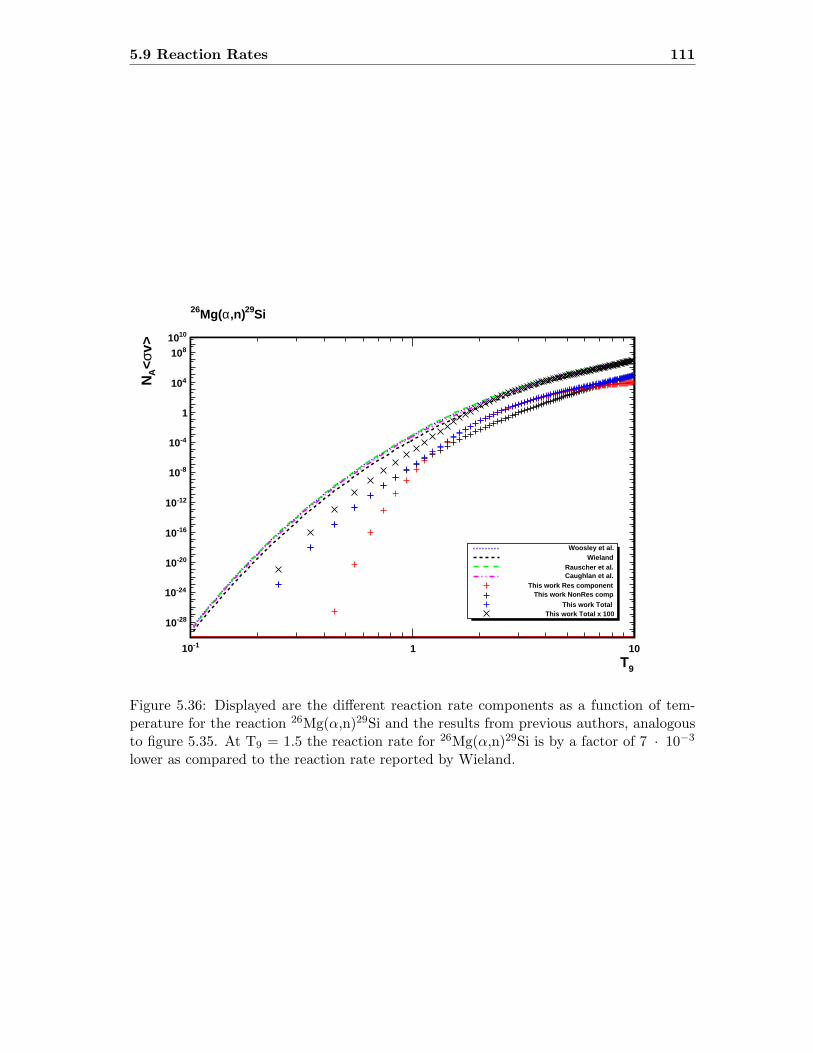
5.9 Reaction Rates 111
9T-110 1 10
v>s<A
N
-2810
-2410
-2010
-1610
-1210
-810
-410
1
410
810
1010
Woosley et al.Wieland
Rauscher et al.Caughlan et al.
This work Res componentThis work NonRes comp
This work Total This work Total x 100
Si29,n)aMg(26
Figure 5.36: Displayed are the different reaction rate components as a function of tem-perature for the reaction 26Mg(α,n)29Si and the results from previous authors, analogousto figure 5.35. At T9 = 1.5 the reaction rate for 26Mg(α,n)29Si is by a factor of 7 · 10−3
lower as compared to the reaction rate reported by Wieland.
112 Experimental Results
The situation for the 18O(α,n)21Ne the reaction rate is illustrated in figure 5.37. Thecalculation of the reaction rate resulted in an increase by a factor of about 4 due to thehigher measured cross sections. The shift in resonance energies does not have an essentialeffect.A comparison of the reaction rate to the reaction rates of 18O(α,γ)22Ne by Dababneh etal. showed a shift for the temperature at which the (α,n) channel is dominating over the(α,γ) channel (see figure 5.38 and table 5.12). The shift is caused by the new experimentaldata available through Dababneh et al. and the reaction rate from this work. Denker,for example, was only able to compare to older results on 18O(α,γ)22Ne [8, 58]. The shiftindicates a release of additional neutron fluxes and an impact on steller nucleosynthesisat an earlier stage of stellar evolution.
Authors Temperature [T9]
Denker et al. 0.6Denker et al., Dababneh et al. 0.62This work, Dababneh et al. 0.52
Table 5.12: List of temperatures at which the 18O(α,n)21Ne reaction starts to dominateover the 18O(α,γ)22Ne reaction[8, 58].
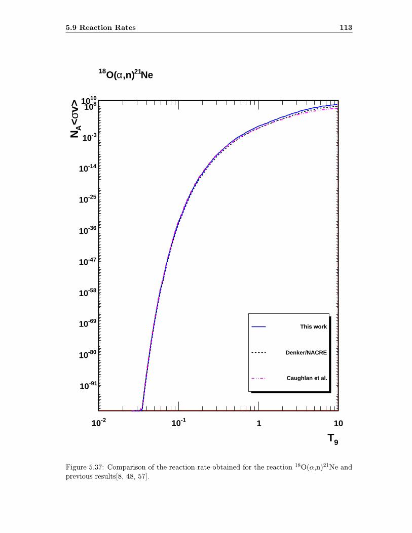
5.9 Reaction Rates 113
9T
-210 -110 1 10
v>s<A
N
-9110
-8010
-6910
-5810
-4710
-3610
-2510
-1410
-310
8101010
This work
Denker/NACRE
Caughlan et al.
Ne21,n)aO(18
Figure 5.37: Comparison of the reaction rate obtained for the reaction 18O(α,n)21Ne andprevious results[8, 48, 57].

114 Experimental Results
9T
-110 1 10
,n)
a(v>s<
A/N )g,a(
v>s<A
N
-510
-310
-110
10
310
510
710
910
1110
1310
1510
(This work),n)a(v>s<AN
(Dababneh et al.))g,a(v>s<AN
(Denker),n)a(v>s<AN
(Dababneh et al.))g,a(v>s<AN
Ne21,n)aO(18
Figure 5.38: Illustrated is the ratio of the obtained reaction rate for 18O(α,n)21Ne to thereaction rate of the (α,γ) channel. The ratio of the reaction rates include the data fromDenker and Dababneh et al.[8, 58].

Chapter 6
Impact Studies
The impact of the previously obtained reactions rates can be quantitavely assessed byimplementing the reaction rates into network calculations (see section 2.4). The PPNNUGRID post-processing code calculates the abundance distribution for each isotope in-volved in the nucleosynthesis processes[30].In the context of this thesis, it is important to note that the results from PPN are based onso-called one-zone calculations. One-zone calculations provide the abundances (and theirvariations) for one given phase of the stellar evolution. 25Mg(α,n)28Si and 26Mg(α,n)29Sibecome relevant during Ne burning conditions, while in the case of 18O(α,n)21Ne, Heburning conditions have to be considered. This constrains the impact of the reactions tospecific aspects of stellar nucleosynthesis.
116 Impact Studies
6.1 25Mg(α,n)28Si & 26Mg(α,n)29Si
The obtained reaction rates of 25Mg(α,n)28Si and 26Mg(α,n)29Si are significantly differentfrom those provided by NACRE[57]. Considering the large uncertainties still associatedwith the reaction rates, a sensitivity study was performed. This study contained thevariation of the reactions rates up to two orders of magnitude in comparison to the reactionrates recommended by NACRE.
To observe the impact of these variations, specific isotopes were chosen, whose abundanceswere estimated to be influenced by the change in reaction rates. Apart from the abun-dances of the Mg and Si isotopes, whose abundances are influenced directly, the isotopicabundances of titanium, strontium, zirconium, molybdenum and barium were chosen asobservables for the impact. The abundances of these isotopes are influenced indirectlythrough the varying neutron exposures.
To account for different initial stellar masses and the Ne-burning conditions in the coreas well as in the convective shell, the calculations were performed at T9 = 1.5 and 1.7.For sake of simplicity, the matter density was kept constant at 106 cm−3. The end ofthe burning phase was conventionally set to the time at which the 20Ne abundance wouldhave dropped to approximately 1%. This would typically be the case after one year for T9
= 1.5, respectively 1.4 days for T9 = 1.7. Notice that under such conditions, convectiveNe-shell burning is terminated by the supernova explosion, while 20Ne is still available[10].
Nucleosynthesis in the pre-explosive Ne-shell is mostly affected by the reactions during theinitial burning phase, when 20Ne is more abundant. As the 20Ne abundance decreases inthe shell, the amounts of α-particles, neutrons and protons rapidly drop as well. For thisreason, the results of our impact study may be applied to both Ne-burning conditions, inthe core (complete 20Ne exhaustion) and in the shell (partial 20Ne exhaustion).
The initial seed abundances for the calculations are taken from the C-burning ashes of aof 25M⊙ and solar-like metallicity star[23].
The calculations provide the abundance distribution at the end of the Ne shell not onlyfor stable but also for unstable isotopes which can contribute to the abundances of thestable isotopes through their β-decays. This additional component is called radiogeniccomponent. The half-life of the contributing isotope has to be long enough to contributeduring the condensation phase of the ejected material, e.g. observed in form of the SiC Xgrains (see secton 2.5).
In figure 6.1, the neutron density is plotted as a function of time during neon burning forthe different cases considered in our study. The maximum neutron density is obtained inthe first phases of Ne burning followed by a rapid decrease. At the beginning, the high20Ne abundance provides a large flux of α-particles via the 20Ne(γ,α)16O reaction.
These α-particles may then be captured by 25Mg and 26Mg to produce neutrons. Theburning of 25Mg and 26Mg via α-capture and the decrease of 20Ne cause the neutrondensity to decrease with time. The different neutron peak densities illustrated in figure6.1 show that 25Mg(α,n)28Si and 26Mg(α,n)29Si provide about 50% of the total neutrondensity as evident by comparing the different cases when their respective reaction ratesare decreased, kept the same or set to zero.
In figures 6.2 - 6.7, the obtained abundance distributions and their variation at the endof Ne shell burning are shown. In most cases, the radiogenic contribution to the stableisotopes is negligible or small compared to the original abundances of the stable species.For a small number of considered cases, however the radiogenic contribution is indeedsignificant, and does affect the final isotopic distribution. The most significant ones are
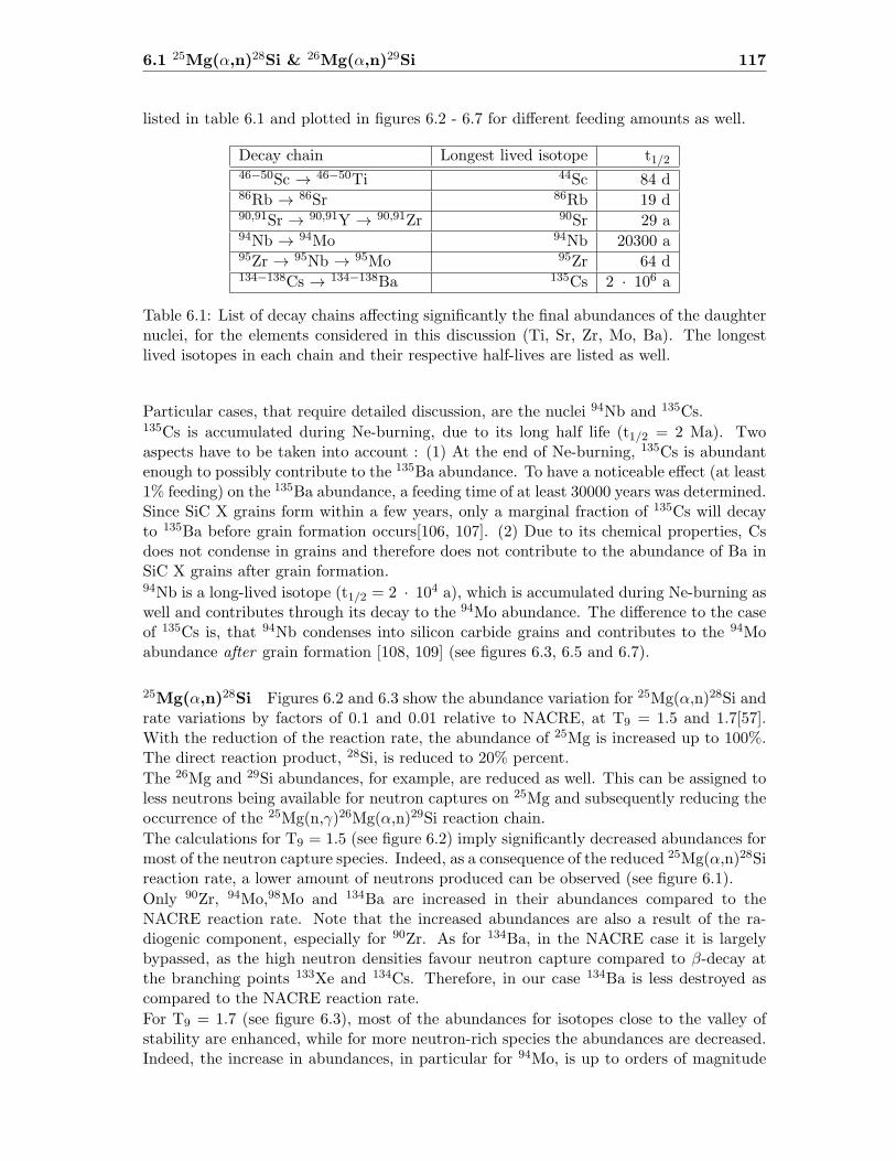
6.1 25Mg(α,n)28Si & 26Mg(α,n)29Si 117
listed in table 6.1 and plotted in figures 6.2 - 6.7 for different feeding amounts as well.
Decay chain Longest lived isotope t1/246−50Sc → 46−50Ti 44Sc 84 d86Rb → 86Sr 86Rb 19 d90,91Sr → 90,91Y → 90,91Zr 90Sr 29 a94Nb → 94Mo 94Nb 20300 a95Zr → 95Nb → 95Mo 95Zr 64 d134−138Cs → 134−138Ba 135Cs 2 · 106 a
Table 6.1: List of decay chains affecting significantly the final abundances of the daughternuclei, for the elements considered in this discussion (Ti, Sr, Zr, Mo, Ba). The longestlived isotopes in each chain and their respective half-lives are listed as well.
Particular cases, that require detailed discussion, are the nuclei 94Nb and 135Cs.135Cs is accumulated during Ne-burning, due to its long half life (t1/2 = 2 Ma). Twoaspects have to be taken into account : (1) At the end of Ne-burning, 135Cs is abundantenough to possibly contribute to the 135Ba abundance. To have a noticeable effect (at least1% feeding) on the 135Ba abundance, a feeding time of at least 30000 years was determined.Since SiC X grains form within a few years, only a marginal fraction of 135Cs will decayto 135Ba before grain formation occurs[106, 107]. (2) Due to its chemical properties, Csdoes not condense in grains and therefore does not contribute to the abundance of Ba inSiC X grains after grain formation.94Nb is a long-lived isotope (t1/2 = 2 · 104 a), which is accumulated during Ne-burning aswell and contributes through its decay to the 94Mo abundance. The difference to the caseof 135Cs is, that 94Nb condenses into silicon carbide grains and contributes to the 94Moabundance after grain formation [108, 109] (see figures 6.3, 6.5 and 6.7).
25Mg(α,n)28Si Figures 6.2 and 6.3 show the abundance variation for 25Mg(α,n)28Si andrate variations by factors of 0.1 and 0.01 relative to NACRE, at T9 = 1.5 and 1.7[57].With the reduction of the reaction rate, the abundance of 25Mg is increased up to 100%.The direct reaction product, 28Si, is reduced to 20% percent.
The 26Mg and 29Si abundances, for example, are reduced as well. This can be assigned toless neutrons being available for neutron captures on 25Mg and subsequently reducing theoccurrence of the 25Mg(n,γ)26Mg(α,n)29Si reaction chain.
The calculations for T9 = 1.5 (see figure 6.2) imply significantly decreased abundances formost of the neutron capture species. Indeed, as a consequence of the reduced 25Mg(α,n)28Sireaction rate, a lower amount of neutrons produced can be observed (see figure 6.1).
Only 90Zr, 94Mo,98Mo and 134Ba are increased in their abundances compared to theNACRE reaction rate. Note that the increased abundances are also a result of the ra-diogenic component, especially for 90Zr. As for 134Ba, in the NACRE case it is largelybypassed, as the high neutron densities favour neutron capture compared to β-decay atthe branching points 133Xe and 134Cs. Therefore, in our case 134Ba is less destroyed ascompared to the NACRE reaction rate.
For T9 = 1.7 (see figure 6.3), most of the abundances for isotopes close to the valley ofstability are enhanced, while for more neutron-rich species the abundances are decreased.Indeed, the increase in abundances, in particular for 94Mo, is up to orders of magnitude

118 Impact Studies
Time [a]-410 -310 -210 -110 1
)-3
(cm
nr
1010
1110
1210
1310
1410
= 1 a, End of Ne shellmax, T-3 cm6= 10r = 1.5 & 1.7 , 9T = 1.59
Si NACRE x1 T28,29
,n)aMg(25,26
= 1.59
Si NACRE x0.1 T28,29
,n)aMg(25,26
= 1.59
Si NACRE x0.01 T25,29
,n)aMg(25,26
= 1.59
Si NACRE x0 T28,29
,n)aMg(25,26
= 1.79
Si NACRE x1 T28,29
,n)aMg(25,26
= 1.79
Si NACRE x0.1 T28,29
,n)aMg(25,26
= 1.79
Si NACRE x0.01 T28,29
,n)aMg(25,26
= 1.79
Si NACRE x0 T28,29
,n)aMg(25,26
Figure 6.1: Neutron density as a function of time for T9 = 1.5 & 1.7. For T9 = 1.7 andafter 1.4 days (3.8 · 10−3 a) the Ne burning phase stops due to the exhaustion of 20 Ne.

6.1 25Mg(α,n)28Si & 26Mg(α,n)29Si 119
higher (depending on the radiogenic feeding) as compared to the case of T9 = 1.5. Thisis caused by the reduced amount of neutrons (caused by the lower reaction rate) availablefor neutron captures as compared to the abundances calculated for the NACRE reactionrate.
26Mg(α,n)29Si The present calculations show a higher sensitivity to the production ofneutrons by 26Mg(α,n)29Si in the Ne shell as compared to 25Mg(α,n)28Si. For exam-ple, at T9 = 1.5 the abundance of 29Si is more reduced with the lower reaction rate on26Mg(α,n)29Si than the 28Si abundance for the 25Mg(α,n)28Si case. Additionally, up to65% less Sr is produced compared to about 45% less for 25Mg(α,n)28Si (see figures 6.4 and6.5). In comparison to 25Mg(α,n)28Si, the abundances of the isotopes are quantitativelymore affected by 26Mg(α,n)29Si, while the general trends are matched by both reactions.
The change in trends between T9 = 1.5 and T9 = 1.7 is the same for both reactions.26Mg(α,n)29Si has a stronger influence on the abundance of the direct reaction productsand the remaining Mg abundances.The quantitative influence of both reactions on the abundance distribution of s-processelement is similar. When adjusting the reaction rates of both reactions at the same timethe effects on the abundance distributions become quantitatively stronger (see figures 6.6and 6.7). The different behaviour between T9 = 1.5 and T9 = 1.7 is due to the differentneutron density regimes found.For T9 = 1.7 an additional feature has to be taken into account. The observation of anincreased abundance of for example the p-only nuclide 92Mo indicates the significance ofphotodesintegrations (e.g. (γ,n) reactions). As the amount of neutrons becomes lowerthrough the decreased reaction rates, the equilibrium between (n,γ) and (γ,n) reactionsis shifted towards the destruction channel (γ,n). Additionally for (γ,n) reactions, one canestimate the time scale by the inverse of the reaction rate (or half-life, respectively).Especially for the phase after 20Ne is exhausted, no neutrons can be supplied to furtherfuel the (α,n) reactions.
Mo isotope Time scale T9 =1.5 [a] Time scale T9 =1.7 [a]
92 2.60E+15 2.06E+10
93 6.60E+02 3.40E-01
94 1.50E+06 1.31E+02
95 2.40E+00 2.40E-03
96 2.56E+04 5.21E+00
97 2.85E-02 4.68E-05
98 4.09E+02 1.32E-01
99 3.25E-05 1.33E-07
100 4.23E+01 1.80E-02
Table 6.2: Listed are the time scales for (γ,n) reactions on the Mo isotopes for T9 =1.5and T9 =1.7. The times scales, in general, are several orders of magnitude smaller forhigher temperature regimes.
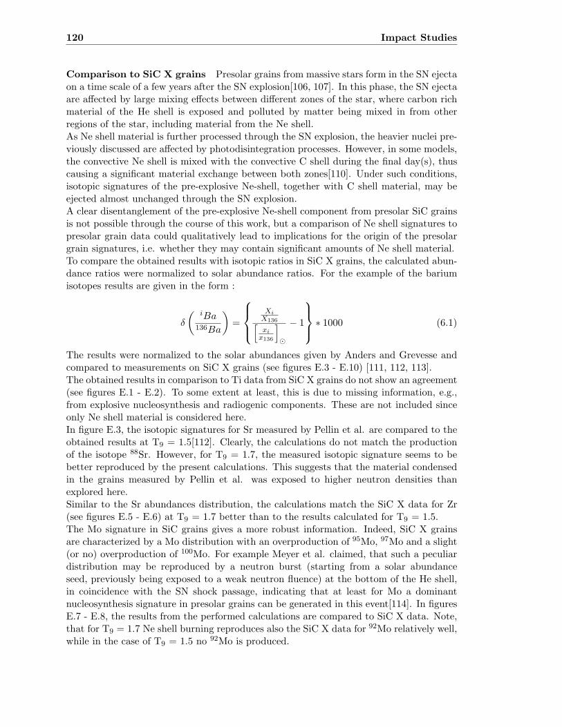
120 Impact Studies
Comparison to SiC X grains Presolar grains from massive stars form in the SN ejectaon a time scale of a few years after the SN explosion[106, 107]. In this phase, the SN ejectaare affected by large mixing effects between different zones of the star, where carbon richmaterial of the He shell is exposed and polluted by matter being mixed in from otherregions of the star, including material from the Ne shell.As Ne shell material is further processed through the SN explosion, the heavier nuclei pre-viously discussed are affected by photodisintegration processes. However, in some models,the convective Ne shell is mixed with the convective C shell during the final day(s), thuscausing a significant material exchange between both zones[110]. Under such conditions,isotopic signatures of the pre-explosive Ne-shell, together with C shell material, may beejected almost unchanged through the SN explosion.A clear disentanglement of the pre-explosive Ne-shell component from presolar SiC grainsis not possible through the course of this work, but a comparison of Ne shell signatures topresolar grain data could qualitatively lead to implications for the origin of the presolargrain signatures, i.e. whether they may contain significant amounts of Ne shell material.To compare the obtained results with isotopic ratios in SiC X grains, the calculated abun-dance ratios were normalized to solar abundance ratios. For the example of the bariumisotopes results are given in the form :
δ
(iBa
136Ba
)=
Xi
X136[xi
x136
]⊙
− 1
∗ 1000 (6.1)
The results were normalized to the solar abundances given by Anders and Grevesse andcompared to measurements on SiC X grains (see figures E.3 - E.10) [111, 112, 113].The obtained results in comparison to Ti data from SiC X grains do not show an agreement(see figures E.1 - E.2). To some extent at least, this is due to missing information, e.g.,from explosive nucleosynthesis and radiogenic components. These are not included sinceonly Ne shell material is considered here.In figure E.3, the isotopic signatures for Sr measured by Pellin et al. are compared to theobtained results at T9 = 1.5[112]. Clearly, the calculations do not match the productionof the isotope 88Sr. However, for T9 = 1.7, the measured isotopic signature seems to bebetter reproduced by the present calculations. This suggests that the material condensedin the grains measured by Pellin et al. was exposed to higher neutron densities thanexplored here.Similar to the Sr abundances distribution, the calculations match the SiC X data for Zr(see figures E.5 - E.6) at T9 = 1.7 better than to the results calculated for T9 = 1.5.The Mo signature in SiC grains gives a more robust information. Indeed, SiC X grainsare characterized by a Mo distribution with an overproduction of 95Mo, 97Mo and a slight(or no) overproduction of 100Mo. For example Meyer et al. claimed, that such a peculiardistribution may be reproduced by a neutron burst (starting from a solar abundanceseed, previously being exposed to a weak neutron fluence) at the bottom of the He shell,in coincidence with the SN shock passage, indicating that at least for Mo a dominantnucleosynthesis signature in presolar grains can be generated in this event[114]. In figuresE.7 - E.8, the results from the performed calculations are compared to SiC X data. Note,that for T9 = 1.7 Ne shell burning reproduces also the SiC X data for 92Mo relatively well,while in the case of T9 = 1.5 no 92Mo is produced.
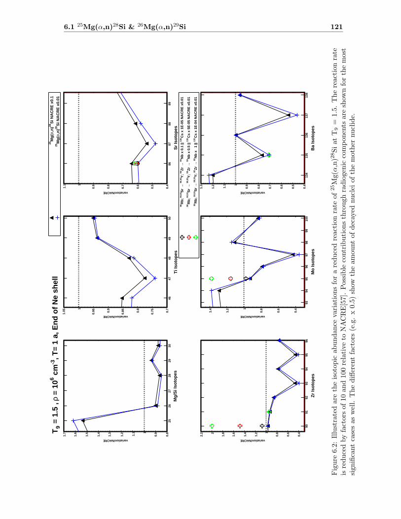
6.1 25Mg(α,n)28Si & 26Mg(α,n)29Si 121
Mg/
Si I
soto
pes
2526
2728
2930
variation/NACRE
0.8
0.91
1.1
1.2
1.3
1.4
1.5
1.6
1.7
Ti I
soto
pes
4647
4849
50
variation/NACRE
0.7
0.750.
8
0.850.
9
0.95
1
1.05
Sr
Isot
opes
8687
8889
variation/NACRE
0.4
0.5
0.6
0.7
0.8
0.91
1.1
Zr
Isot
opes
9091
9293
9495
96
variation/NACRE
0.4
0.6
0.81
1.2
1.4
1.6
1.82
2.2
Mo
Isot
opes
9394
9596
9798
9910
0
variation/NACRE
0.4
0.6
0.81
1.2
1.4
Ba
Isot
opes
134
135
136
137
138
variation/NACRE
0.4
0.5
0.6
0.7
0.8
0.91
1.1
1.2
1.3
, T=
1 a,
End
of N
e sh
ell
-3 c
m6
= 1
0r
= 1
.5 ,
9T
Si N
AC
RE
x0.
128
,n)
aM
g(25
Si N
AC
RE
x0.
0128
,n)
aM
g(25
Cs
x 1E
-05
NA
CR
E x
0.01
135
Nb
x 0.
1 ||
95 ®
Zr
95Y
; 90
,91
®
Sr
90,9
1R
b;
86
Cs
x 5E
-05
NA
CR
E x
0.01
135
Nb
x 0.
5 ||
95 ®
Zr
95Y
; 90
,91
®
Sr
90,9
1R
b;
86
Cs
x 1E
-04
NA
CR
E x
0.01
135
Nb
x 1
||
95 ®
Zr
95Y
; 90
,91
®
Sr
90,9
1R
b;
86
Figure
6.2:
Illustratedaretheisotop
icab
undan
cevariationsforareducedreactionrate
of25Mg(α
,n)2
8SiatT9=
1.5.Thereactionrate
isreducedbyfactorsof
10an
d100relativeto
NACRE[57].Possible
contributionsthroughradiogenic
components
are
show
nforthemost
sign
ificantcasesas
well.Thedifferentfactors(e.g.x0.5)show
theamountofdecayed
nuclei
ofthemother
nuclide.
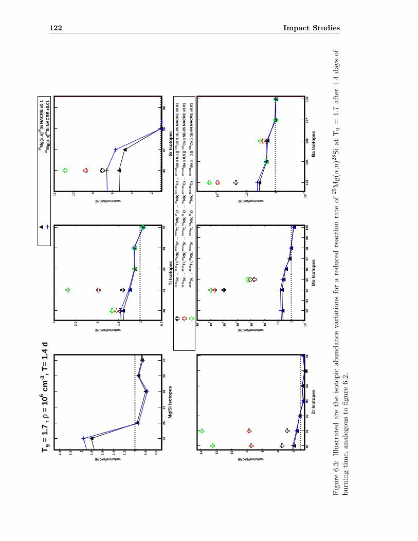
122 Impact Studies
Mg/
Si I
soto
pes
2526
2728
2930
variation/NACRE
0.6
0.81
1.2
1.4
1.6
1.82
2.2
2.4
Ti I
soto
pes
4647
4849
50
variation/NACRE
0.51
1.52
2.53
Sr
Isot
opes
8687
8889
variation/NACRE
24681012
Zr
Isot
opes
9091
9293
9495
96
variation/NACRE
2468101214
Mo
Isot
opes
9293
9495
9697
9899
100
variation/NACRE
-110
1
10
210
310
410
510
610
710
Ba
Isot
opes
134
135
136
137
138
variation/NACRE
-110
1
10
210
, T=
1.4
d-3
cm
6 =
10
r =
1.7
, 9
TS
i NA
CR
E x
0.1
28,n
)a
Mg(
25
Si N
AC
RE
x0.
0128
,n)
aM
g(25
Cs
x 1E
-05
NA
CR
E x
0.01
135
Ba
x 0.
1 ||
134-
138
®
Cs
134-
138
Nb;
95
®Z
r 95
Nb;
94
Y;
90,9
1
®S
r 90
,91
Rb;
86
Ti;
46-5
0
®S
c 46
-50
Cs
x 5E
-05
NA
CR
E x
0.01
135
Ba
x 0.
5 ||
134-
138
®
Cs
134-
138
Nb;
95
®Z
r 95
Nb;
94
Y;
90,9
1
®S
r 90
,91
Rb;
86
Ti;
46-5
0
®S
c 46
-50
Cs
x 1E
-04
NA
CR
E x
0.01
135
Ba
x
1 ||
134-
138
®
Cs
134-
138
Nb;
95
®Z
r 95
Nb;
94
Y;
90,9
1
®S
r 90
,91
Rb;
86
Ti;
46-5
0
®S
c 46
-50
Figure
6.3:
Illustratedaretheisotop
icab
undan
cevariationsforareducedreactionrate
of25Mg(α
,n)2
8Siat
T9=
1.7after1.4day
sof
burningtime,
analogou
sto
figu
re6.2.
6.1 25Mg(α,n)28Si & 26Mg(α,n)29Si 123
Mg/
Si I
soto
pes
2526
2728
2930
variation/NACRE
0.51
1.52
2.53
3.54
Ti I
soto
pes
4647
4849
50
variation/NACRE
0.6
0.650.
7
0.750.
8
0.850.
9
0.95
1
1.05
Sr
Isot
opes
8687
8889
variation/NACRE
0.4
0.5
0.6
0.7
0.8
0.91
1.1
Zr
Isot
opes
9091
9293
9495
96
variation/NACRE
0.4
0.6
0.81
1.2
1.4
1.6
1.82
Mo
Isot
opes
9394
9596
9798
9910
0
variation/NACRE
0.2
0.4
0.6
0.81
1.2
1.4
Ba
Isot
opes
134
135
136
137
138
variation/NACRE
0.4
0.5
0.6
0.7
0.8
0.91
1.1
1.2
1.3
, T=
1 a,
End
of N
e sh
ell
-3 c
m6
= 1
0r
= 1
.5 ,
9T
Si N
AC
RE
x0.
129
,n)
aM
g(26
Si N
AC
RE
x0.
0129
,n)
aM
g(26
Cs
x 1E
-05
NA
CR
E x
0.01
135
Nb
x 0.
1 ||
95 ®
Zr
95Y
; 90
,91
®
Sr
90,9
1R
b;
86
Cs
x 5E
-05
NA
CR
E x
0.01
135
Nb
x 0.
5 ||
95 ®
Zr
95Y
; 90
,91
®
Sr
90,9
1R
b;
86
Cs
x 1E
-04
NA
CR
E x
0.01
135
Nb
x 1
||
95 ®
Zr
95Y
; 90
,91
®
Sr
90,9
1R
b;
86
Figure
6.4:
Illustratedaretheisotop
icab
undan
cevariationsforareducedreactionrate
of26Mg(α
,n)2
9SiatT9=
1.5,analogousto
figure
6.2.
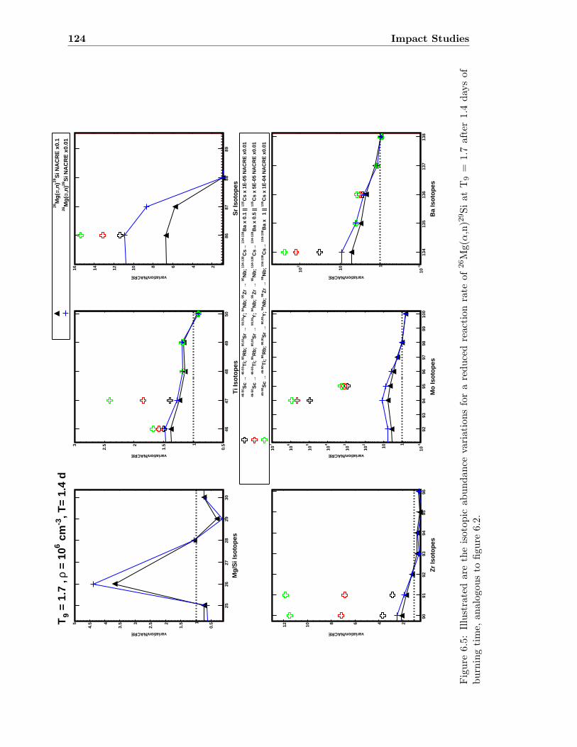
124 Impact Studies
Mg/
Si I
soto
pes
2526
2728
2930
variation/NACRE
0.51
1.52
2.53
3.54
4.55
Ti I
soto
pes
4647
4849
50
variation/NACRE
0.51
1.52
2.53
Sr
Isot
opes
8687
8889
variation/NACRE
246810121416
Zr
Isot
opes
9091
9293
9495
96
variation/NACRE
24681012
Mo
Isot
opes
9293
9495
9697
9899
100
variation/NACRE
-110
1
10
210
310
410
510
610
710
Ba
Isot
opes
134
135
136
137
138
variation/NACRE
-110
1
10
210
, T=
1.4
d-3
cm
6 =
10
r =
1.7
, 9
TS
i NA
CR
E x
0.1
29,n
)a
Mg(
26
Si N
AC
RE
x0.
0129
,n)
aM
g(26
Cs
x 1E
-05
NA
CR
E x
0.01
135
Ba
x 0.
1 ||
134-
138
®
Cs
134-
138
Nb;
95
®Z
r 95
Nb;
94
Y;
90,9
1
®S
r 90
,91
Rb;
86
Ti;
46-5
0
®S
c 46
-50
Cs
x 5E
-05
NA
CR
E x
0.01
135
Ba
x 0.
5 ||
134-
138
®
Cs
134-
138
Nb;
95
®Z
r 95
Nb;
94
Y;
90,9
1
®S
r 90
,91
Rb;
86
Ti;
46-5
0
®S
c 46
-50
Cs
x 1E
-04
NA
CR
E x
0.01
135
Ba
x 1
||
134-
138
®
Cs
134-
138
Nb;
95
®Z
r 95
Nb;
94
Y;
90,9
1
®S
r 90
,91
Rb;
86
Ti;
46-5
0
®S
c 46
-50
Figure
6.5:
Illustratedaretheisotop
icab
undan
cevariationsforareducedreactionrate
of26Mg(α
,n)2
9Siat
T9=
1.7after1.4day
sof
burningtime,
analogou
sto
figu
re6.2.
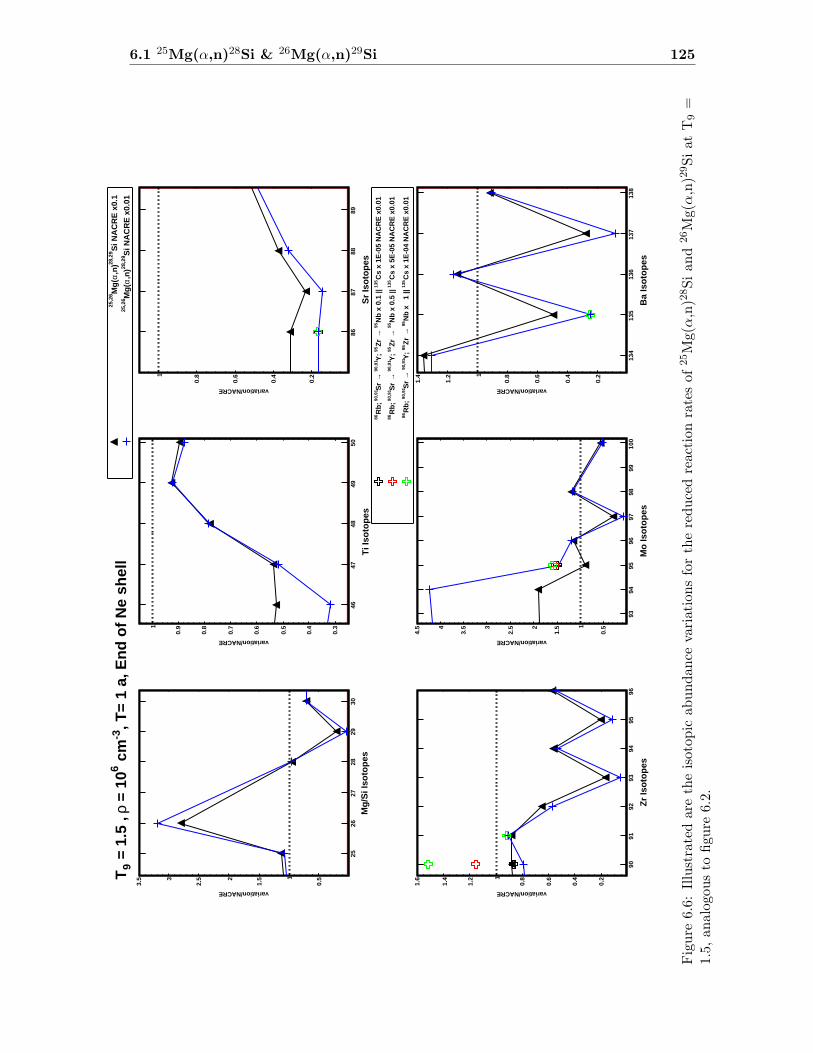
6.1 25Mg(α,n)28Si & 26Mg(α,n)29Si 125
Mg/
Si I
soto
pes
2526
2728
2930
variation/NACRE
0.51
1.52
2.53
3.5
Ti I
soto
pes
4647
4849
50
variation/NACRE
0.3
0.4
0.5
0.6
0.7
0.8
0.91
Sr
Isot
opes
8687
8889
variation/NACRE
0.2
0.4
0.6
0.81
Zr
Isot
opes
9091
9293
9495
96
variation/NACRE
0.2
0.4
0.6
0.81
1.2
1.4
1.6
Mo
Isot
opes
9394
9596
9798
9910
0
variation/NACRE
0.51
1.52
2.53
3.54
4.5
Ba
Isot
opes
134
135
136
137
138
variation/NACRE
0.2
0.4
0.6
0.81
1.2
1.4
, T=
1 a,
End
of N
e sh
ell
-3 c
m6
= 1
0r
= 1
.5 ,
9T
Si N
AC
RE
x0.
128
,29
,n)
aM
g(25
,26
Si N
AC
RE
x0.
0128
,29
,n)
aM
g(25
,26
Cs
x 1E
-05
NA
CR
E x
0.01
135
Nb
x 0.
1 ||
95 ®
Zr
95Y
; 90
,91
®
Sr
90,9
1R
b;
86
Cs
x 5E
-05
NA
CR
E x
0.01
135
Nb
x 0.
5 ||
95 ®
Zr
95Y
; 90
,91
®
Sr
90,9
1R
b;
86
Cs
x 1E
-04
NA
CR
E x
0.01
135
Nb
x 1
||
95 ®
Zr
95Y
; 90
,91
®
Sr
90,9
1R
b;
86
Figure
6.6:
Illustratedaretheisotop
icab
undance
variationsforthereducedreactionratesof25Mg(α
,n)2
8Siand
26Mg(α
,n)2
9SiatT9=
1.5,
analogou
sto
figu
re6.2.
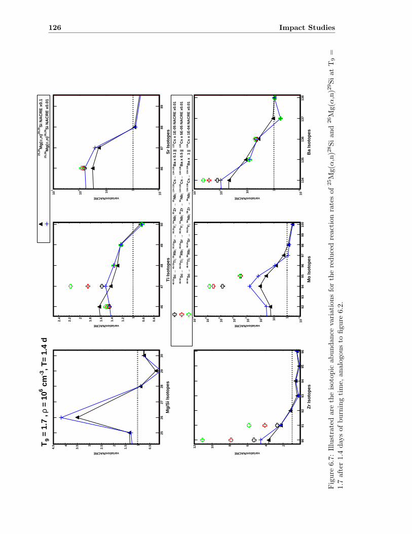
126 Impact Studies
Mg/
Si I
soto
pes
2526
2728
2930
variation/NACRE
0.51
1.52
2.53
3.54
4.5
Ti I
soto
pes
4647
4849
50
variation/NACRE
0.6
0.81
1.2
1.4
1.6
1.82
2.2
2.4
Sr
Isot
opes
8687
8889
variation/NACRE
-110
1
10
210
310
Zr
Isot
opes
9091
9293
9495
96
variation/NACRE
24681012
Mo
Isot
opes
9293
9495
9697
9899
100
variation/NACRE
-110
1
10
210
310
410
510
610
710
Ba
Isot
opes
134
135
136
137
138
variation/NACRE
-110
1
10
210
310
, T=
1.4
d-3
cm
6 =
10
r =
1.7
, 9
TS
i NA
CR
E x
0.1
28,2
9,n
)a
Mg(
25,2
6
Si N
AC
RE
x0.
0128
,29
,n)
aM
g(25
,26
Cs
x 1E
-05
NA
CR
E x
0.01
135
Ba
x 0.
1 ||
13
4-13
8
®C
s13
4-13
8N
b;
95 ®
Zr
95N
b;
94Y
; 90
,91
®
Sr
90,9
1R
b;
86T
i; 46
-50
®
Sc
46-5
0
Cs
x 5E
-05
NA
CR
E x
0.01
135
Ba
x 0.
5 ||
13
4-13
8
®C
s13
4-13
8N
b;
95 ®
Zr
95N
b;
94Y
; 90
,91
®
Sr
90,9
1R
b;
86T
i; 46
-50
®
Sc
46-5
0
Cs
x 1E
-04
NA
CR
E x
0.01
135
Ba
x 1
||
134-
138
®
Cs
134-
138
Nb;
95
®Z
r 95
Nb;
94
Y;
90,9
1
®S
r 90
,91
Rb;
86
Ti;
46-5
0
®S
c 46
-50
Figure
6.7:
Illustratedaretheisotop
icab
undan
cevariationsforthereducedreactionratesof25Mg(α,n)2
8Sian
d26Mg(α,n)2
9Siat
T9=
1.7after1.4day
sof
burningtime,
analogou
sto
figu
re6.2.

6.1 25Mg(α,n)28Si & 26Mg(α,n)29Si 127
The results from the calculations and the measured Ba signatures are compared in figuresE.9 and E.10. The calculations reproduce the abundance of 138Ba only at a temperatureof T9= 1.7.To explain the isotopic anomalies in grain KJB2-11-17-1, Hoppe et al. proposed an in-crease of the NACRE reaction rate of 26Mg(α,n)29Si by a factor of two[54, 57]. As theexperimental results for the reaction rate do show a decrease rather than an increase, abrief comparison with the calculated abundances is listed in table 6.3. Indeed, for thedecreased reaction rates of 25Mg(α,n)28Si and 26Mg(α,n)29Si, the calculated 29Si abun-dance seem to be in the same order for NACRE x 0.1 and T9= 1.7. But, in contrast, the30Si abundances differ substantially as compared to the ones found in grain KJB2-11-17-1.Calculations, in which only the reaction rate of 26Mg(α,n)29Si was varied, were performedas well, but showed no improvement.These results imply that the Si isotopes in this grain have not been synthesized duringNe burning alone. This conclusion is in accordance Hoppe et al. who note, that mixingbetween oxygen and neon zone has to be taken into account. However, the abundancescalculated with the current data set only for the O/Ne zone also provide no match betweenthe data sets.On the other hand, due to the lower reaction rates, more 25Mg and 26Mg are left in theashes of Ne burning, which then can be processed during further burning stages, such asoxygen burning or explosive burning phases. This could also have interesting implicationsfor explosive nucleosynthesis calculations in massive stars and influence the final outcomeof the resulting abundances. A more conclusive picture may be obtained by performingthe same type of mixing calculations as Hoppe et al. did, but with the decreased reactionrates of 25Mg(α,n)28Si and 26Mg(α,n)29Si. This is beyond the scope of this thesis.
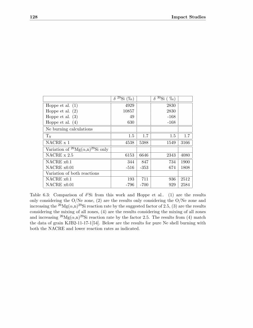
128 Impact Studies
δ 29Si (h) δ 30Si ( h)
Hoppe et al. (1) 4929 2830Hoppe et al. (2) 10857 2830Hoppe et al. (3) 49 -168Hoppe et al. (4) 630 -168
Ne burning calculations
T9 1.5 1.7 1.5 1.7
NACRE x 1 4538 5388 1549 3166
Variation of 26Mg(α,n)29Si only
NACRE x 2.5 6153 6646 2343 4080
NACRE x0.1 344 847 734 1900NACRE x0.01 -516 -353 674 1808
Variation of both reactions
NACRE x0.1 193 711 936 2512NACRE x0.01 -796 -700 929 2584
Table 6.3: Comparison of δiSi from this work and Hoppe et al.. (1) are the resultsonly considering the O/Ne zone, (2) are the results only considering the O/Ne zone andincreasing the 26Mg(α,n)29Si reaction rate by the suggested factor of 2.5, (3) are the resultsconsidering the mixing of all zones, (4) are the results considering the mixing of all zonesand increasing 26Mg(α,n)29Si reaction rate by the factor 2.5. The results from (4) matchthe data of grain KJB2-11-17-1[54]. Below are the results for pure Ne shell burning withboth the NACRE and lower reaction rates as indicated.
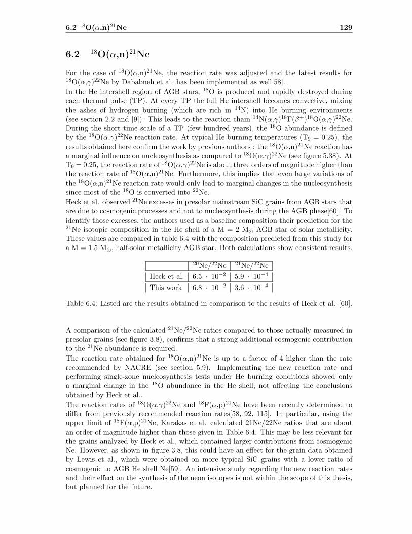
6.2 18O(α,n)21Ne 129
6.2 18O(α,n)21Ne
For the case of 18O(α,n)21Ne, the reaction rate was adjusted and the latest results for18O(α,γ)22Ne by Dababneh et al. has been implemented as well[58].
In the He intershell region of AGB stars, 18O is produced and rapidly destroyed duringeach thermal pulse (TP). At every TP the full He intershell becomes convective, mixingthe ashes of hydrogen burning (which are rich in 14N) into He burning environments(see section 2.2 and [9]). This leads to the reaction chain 14N(α,γ)18F(β+)18O(α,γ)22Ne.During the short time scale of a TP (few hundred years), the 18O abundance is definedby the 18O(α,γ)22Ne reaction rate. At typical He burning temperatures (T9 = 0.25), theresults obtained here confirm the work by previous authors : the 18O(α,n)21Ne reaction hasa marginal influence on nucleosynthesis as compared to 18O(α,γ)22Ne (see figure 5.38). AtT9 = 0.25, the reaction rate of 18O(α,γ)22Ne is about three orders of magnitude higher thanthe reaction rate of 18O(α,n)21Ne. Furthermore, this implies that even large variations ofthe 18O(α,n)21Ne reaction rate would only lead to marginal changes in the nucleosynthesissince most of the 18O is converted into 22Ne.
Heck et al. observed 21Ne excesses in presolar mainstream SiC grains from AGB stars thatare due to cosmogenic processes and not to nucleosynthesis during the AGB phase[60]. Toidentify those excesses, the authors used as a baseline composition their prediction for the21Ne isotopic composition in the He shell of a M = 2 M⊙ AGB star of solar metallicity.These values are compared in table 6.4 with the composition predicted from this study fora M = 1.5 M⊙, half-solar metallicity AGB star. Both calculations show consistent results.
20Ne/22Ne 21Ne/22Ne
Heck et al. 6.5 · 10−2 5.9 · 10−4
This work 6.8 · 10−2 3.6 · 10−4
Table 6.4: Listed are the results obtained in comparison to the results of Heck et al. [60].
A comparison of the calculated 21Ne/22Ne ratios compared to those actually measured inpresolar grains (see figure 3.8), confirms that a strong additional cosmogenic contributionto the 21Ne abundance is required.
The reaction rate obtained for 18O(α,n)21Ne is up to a factor of 4 higher than the raterecommended by NACRE (see section 5.9). Implementing the new reaction rate andperforming single-zone nucleosynthesis tests under He burning conditions showed onlya marginal change in the 18O abundance in the He shell, not affecting the conclusionsobtained by Heck et al..
The reaction rates of 18O(α,γ)22Ne and 18F(α,p)21Ne have been recently determined todiffer from previously recommended reaction rates[58, 92, 115]. In particular, using theupper limit of 18F(α,p)21Ne, Karakas et al. calculated 21Ne/22Ne ratios that are aboutan order of magnitude higher than those given in Table 6.4. This may be less relevant forthe grains analyzed by Heck et al., which contained larger contributions from cosmogenicNe. However, as shown in figure 3.8, this could have an effect for the grain data obtainedby Lewis et al., which were obtained on more typical SiC grains with a lower ratio ofcosmogenic to AGB He shell Ne[59]. An intensive study regarding the new reaction ratesand their effect on the synthesis of the neon isotopes is not within the scope of this thesis,but planned for the future.

130 Impact Studies
The competition between the reactions 18O(α,n)21Ne and 18O(α,γ)22Ne does not playa role in more advanced burning phases (and therefore higher temperatures) as 18O iscompletely destroyed in the early stages of He-burning.
Chapter 7
Conclusions
During the course of this thesis, a more complete picture on the impact of the reac-tions 25Mg(α,n)28Si, 26Mg(α,n)29Si and 18O(α,n)21Ne on stellar nucleosynthesis has beenachieved.
25Mg(α,n)28Si & 26Mg(α,n)29Si For the reactions 25Mg(α,n)28Si and 26Mg(α,n)29Siit was shown that previous results were not accurate enough and needed further im-provement. The improvements undertaken were the development of a more sophisticatedneutron detection system and an advanced analysis method for the experimental data.Furthermore, various ways for the production of solid state targets were investigated andoptimized.Unfortunately, the measurements did not allow a successful separation of the experimentaldata from occuring background reactions at energies of astrophysical interest. It was shownthat these background reactions result from impurities in the targets, not only resultingfrom carbon and oxygen impurites, but also from boron contaminations.For future experiments on 25Mg(α,n)28Si and 26Mg(α,n)29Si, it will be crucial to removethese impurities during the target production process. A removal of the carbon andoxygen impurities is possible, but technically challenging. For example, one could operatethe experimental beam line at vacuum levels of about 10−9 Pa to avoid an oxidation of theMg target layer[99]. Sophisticated tests have to be undertaken for the removal of carbonimpurities. Tode et al., for example, showed, that with an Ar excimer lamp it is possibleto remove carbon contaminations on silicon wafers[117]. Along with the removal of boron,these measures would have to be performed in a vacuum system, which would allow thetransfer of the target to the experimental beamline without leaving the vacuum.An additional improvement would be the use of a germanium detector, operated in coinci-dence with a neutron detector. The germanium detector would constrain the experimentaldata by separating the γ-rays of interest from the ones released by background reactions.A disadvantage of the method would be the decreased efficiency and possible damage ofthe Ge crystal by the neutron irradiation. Additionally, the moderation times of the re-leased neutrons have to be determined carefully to allow the set up of sufficient coincidencewindows.Concerning stellar nucleosynthesis, for the first time a quantitative assessment of theimpact of the reaction rates has been achieved based on the obtained experimental results.The influence of the reaction 25Mg(α,n)28Si can be described as similar compared to thereaction 26Mg(α,n)29Si. While network calculations covered the Ne burning phase, theresulting seed composition for the following phases of stellar evolution is affected as well,
132 Conclusions
which in turn influences also the isotopic abundance distribution in presolar SiC X grains.This aspect, also concerning the synthesis of the Si isotopes, has been addressed brieflybut requires a more advanced study of stellar nucleosynthesis after Ne burning. Probablyonly the implementation of explosive synthesis will allow a final statement concerning thecomposition of presolar SiC X grains. Due to the lack of experimental information on the(α,γ) channel, competition effects between the (α,n) and (α,γ) remain unresolved.
18O(α,n)21Ne The experimental investigation of the 18O(α,n)21Ne reaction only showeda marginal influence of background reactions. For the first time, the experimental mea-surements of Denker were independently confirmed in their trend and were scaled by afactor of four[8]. A reduction of the carbon contamination would be desirable to resolveclearly the resonances and their parameters below Eα = 1100 keV.The impact of the reaction 18O(α,n)21Ne has been investigated with the newly obtainedreaction rates as well. The competition with the 18O(α,γ)22Ne channel turned out tobe critical at a lower stellar temperature than previously reported. It could be shownhowever, that at temperatures, at which the 18O(α,n)21Ne reaction starts to dominateover the 18O(α,γ)22Ne reaction, no 18O would be available due to its exhaustion in theHe-intershell phase. Resulting Ne isotopic abundances are similar to previously obtainedvalues. This confirms that the observed 21Ne excesses in large presolar SiC grains can beassigned to cosmogenic processes and do not have a stellar origin[60].
The challenges and results presented through the course of this thesis have revealed newinsights concerning the investigation of neutron releasing reactions. Especially the devel-opment of a detection system and targets revealed new effects and sources of experimentaluncertainties. To resolve these uncertainties, technologies from other fields, such as solidstate physics, need to be implemented. Despite these challenges, it could be shown, howthe investigated reactions influence the synthesis of elements in specific stellar enviromentsand how sensitive the results are to nuclear physics data. The goal of assessing the im-pact of the investigated reactions on stellar nucleosynthesis was achieved by connectingthe research performed experimentally with theoretical calculations and measurements onpresolar grains. In the future, this approach will allow the quantitative description of theimportance of nuclear reactions for stellar nucleosynthesis.

Appendix A
Beam Tuning Procedures
A.1 Energy Change
1. Calculate new NMR setting via energy calibration function :
NMR = 53.54 · 2 ·√
E(keV)
2. Use coarse and fine of the master reference to reduce the magnetic field in the analyzingmagnet.
• As you go down in particle energy, you will need to keep the accelerator stabilizerbalanced by either extending the corona points or reducing the terminal charge.
• Roughly every 100 keV, adjust the focus of the ion source to maximize the beamcurrent on the beamstop.
• If you go below the desired target frequency, do not go up with the master reference.This will cause hysteresis effects. You must recycle the analyzing magnet.
3. At the desired NMR frequency :
• Adjust the focus of the ion source to maximize beam current on the beam stop.
• Reduce the setting for the Y-steerers (Y1 and Y2) simultaneously to maximize thecurrent on the beamstop.
A.2 Tuning Process for α-Beam
• Balance the current reading on the defining slits by adjusting the X-steerers (X1 andX2).
• Adjust the focus of the ion sources to maximize the beam current on the beamstop.
• Adjust the Y-steerers such that Y-upper and Y-lower are reading a balanced currentand that at the same time the entrance slits to the switching magnet read a balancedcurrent.

134 Beam Tuning Procedures
• Change to the beam profile monitor located in the target room (see A.3).
• Turn down the quadrupoles in the target room.
• Use the beamline steerers X and Y (rastering offsets) and wobblers to get a maximumof 0.5 µA on each of the target slits (C,D,E and F on the aux. meter panel).
• Do not use beamline steerers X1, Y1 and the vertical steerer of the switching magnet.
A.3 Switch to Beam Profile Monitor (BPM) in Target Room
• Do not change channel positions while the BPMs are running.
• BPM setting for channel 2 : position 1 is the BMP in the accelerator vault whileposition 4 is the BPM located in the target room.
• Turn off BPM 2.
• Change channel 2 to desired position
• Turn on BPM 2.
• Adjust the gain of BPM2.
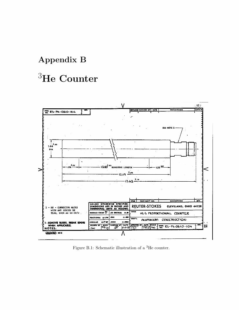
Appendix B
3He Counter
Figure B.1: Schematic illustration of a 3He counter.

Appendix C
Correction Formalism
In this section, the method for the background correction described in section 5.4.2 isbriefly discussed. The general formalism for the experimental yield etc. can be found inreference[27].The experimental yield of a nuclear reaction is given by :
Y = σ · ∆ϵ
(C.1)
where σ is the cross section, ∆ the target thickness and ϵ the stopping power. As oneanalyzes the experimental data one has to determine whether a thin or a thick target ispresent. In general, a thick target can be assumed if the target thickness is at least 6 timesthe natural resonance width.For a thin target the thin-target yield becomes :
Y (E0) =
∫ E0
E0−∆
σ(E)
ϵ(E)dE (C.2)
If ∆ ≫ Γ, the yield becomes
Y (E0) =λ2
2πωγ
M +m
M
1
ϵarctan(E0 − ER
Γ/2)− arctan(
E0 − ER −∆
Γ/2) (C.3)
with M and m as the respective target and projectile masses. If a background componentin form of a resonance peak occurs within the experimental data, one has to determinethe thickness of the component first. By simply fitting the resonance peak with equationC.3 one can either determine the thickness, or if not possible, use the relation :
nt =2
(ωγ)· 1
λ2· I (C.4)
where nt denotes the number of target atoms and I the integral over the peak region[118].The measured experimental data at first is recorded in detected neutrons per incomingalpha particles. Since the background contributions already appear in this stage of theanalysis, it was decided to apply the background corrections at the earliest stage. Gener-ally, the corrected yield would then be :
Yc = Ymeasured − Ybackground (C.5)
Since literature does not report experimental yields but cross sections (or S-factors), theliterature data had to be convoluted into experimental yield data. This was done by
137
calculating the experimental yield via the previous equations. For example, the stoppingpower was then varied assuming different compositions of the targets. The absolute crosssection is defined as :
σ =Nnϵ
Nαϵdet∆(C.6)
with Nn being the detected neutrons, Nα the number of incoming α-particles and thedetection efficiency ϵdet. For the non-resonant part this allows then to caculate the exper-imental yield data for the background components. For the resonances occuring one hasthen to separate the non-resonant and resonant part and use the step function :
Ymax(∞) =λ2
2ωγ
M +m
M
1
ϵ(C.7)
as well, to determine the shape of the resonance peak for a given target thickness andresonance strength. One should take the natural enrichment of the background componentinto account as well.Since the energies in the literature may deviate from the measured energies, an interpola-tion routine was implemented, which interpolates the background yield at the experimen-tally measured energies. The last step is then to apply an energy shift according to thepeak position of the background resonance peak.
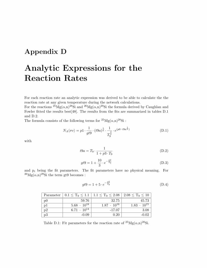
Appendix D
Analytic Expressions for theReaction Rates
For each reaction rate an analytic expression was derived to be able to calculate the thereaction rate at any given temperature during the network calculations.For the reactions 25Mg(α,n)28Si and 26Mg(α,n)29Si the formula derived by Caughlan andFowler fitted the results best[48]. The results from the fits are summarized in tables D.1and D.2.The formula consists of the following terms for 25Mg(α,n)28Si :
NA⟨σv⟩ = p1 · 1
gt9· (t9a)
56 · 1
T329
· e(p0 · t9a13 ) (D.1)
with
t9a = T9 ·1
1 + p3 ·T9(D.2)
gt9 = 1 +10
3· e−
p2T9 (D.3)
and pi being the fit parameters. The fit parameters have no physical meaning. For26Mg(α,n)29Si the term gt9 becomes :
gt9 = 1 + 5 · e−p2T9 (D.4)
Parameter 0.1 ≤ T9 ≤ 1.1 1.1 ≤ T9 ≤ 2.08 2.08 ≤ T9 ≤ 10
p0 59.76 32.75 45.73
p1 5.68 · 1018 1.87 · 1016 1.83 · 1015
p2 6.71 · 1014 -17.07 3.08
p3 -0.09 0.20 -0.02
Table D.1: Fit parameters for the reaction rate of 25Mg(α,n)28Si.
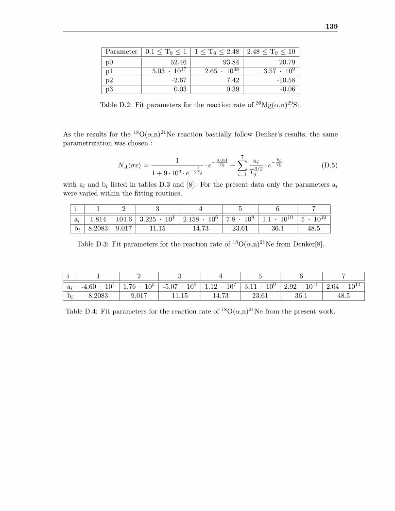
139
Parameter 0.1 ≤ T9 ≤ 1 1 ≤ T9 ≤ 2.48 2.48 ≤ T9 ≤ 10
p0 52.46 93.84 20.79
p1 5.03 · 1017 2.65 · 1038 3.57 · 109
p2 -2.67 7.42 -10.58
p3 0.03 0.39 -0.06
Table D.2: Fit parameters for the reaction rate of 26Mg(α,n)29Si.
As the results for the 18O(α,n)21Ne reaction bascially follow Denker’s results, the sameparametrization was chosen :
NA⟨σv⟩ =1
1 + 9 · 103 · e−1
2T9
· e−8.014T9 +
7∑i=1
ai
T3/29
· e−biT9 (D.5)
with ai and bi listed in tables D.3 and [8]. For the present data only the parameters aiwere varied within the fitting routines.
i 1 2 3 4 5 6 7
ai 1.814 104.6 3.225 · 104 2.158 · 106 7.8 · 108 1.1 · 1010 5 · 1010
bi 8.2083 9.017 11.15 14.73 23.61 36.1 48.5
Table D.3: Fit parameters for the reaction rate of 18O(α,n)21Ne from Denker[8].
i 1 2 3 4 5 6 7
ai -4.60 · 104 1.76 · 105 -5.07 · 105 1.12 · 107 3.11 · 109 2.92 · 1011 2.04 · 1011
bi 8.2083 9.017 11.15 14.73 23.61 36.1 48.5
Table D.4: Fit parameters for the reaction rate of 18O(α,n)21Ne from the present work.
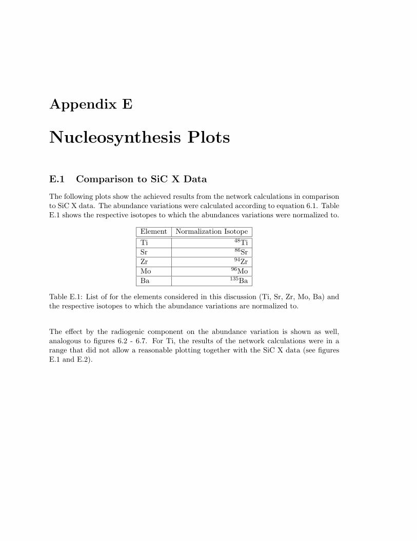
Appendix E
Nucleosynthesis Plots
E.1 Comparison to SiC X Data
The following plots show the achieved results from the network calculations in comparisonto SiC X data. The abundance variations were calculated according to equation 6.1. TableE.1 shows the respective isotopes to which the abundances variations were normalized to.
Element Normalization Isotope
Ti 48Ti
Sr 86Sr
Zr 94Zr
Mo 96Mo
Ba 135Ba
Table E.1: List of for the elements considered in this discussion (Ti, Sr, Zr, Mo, Ba) andthe respective isotopes to which the abundance variations are normalized to.
The effect by the radiogenic component on the abundance variation is shown as well,analogous to figures 6.2 - 6.7. For Ti, the results of the network calculations were in arange that did not allow a reasonable plotting together with the SiC X data (see figuresE.1 and E.2).
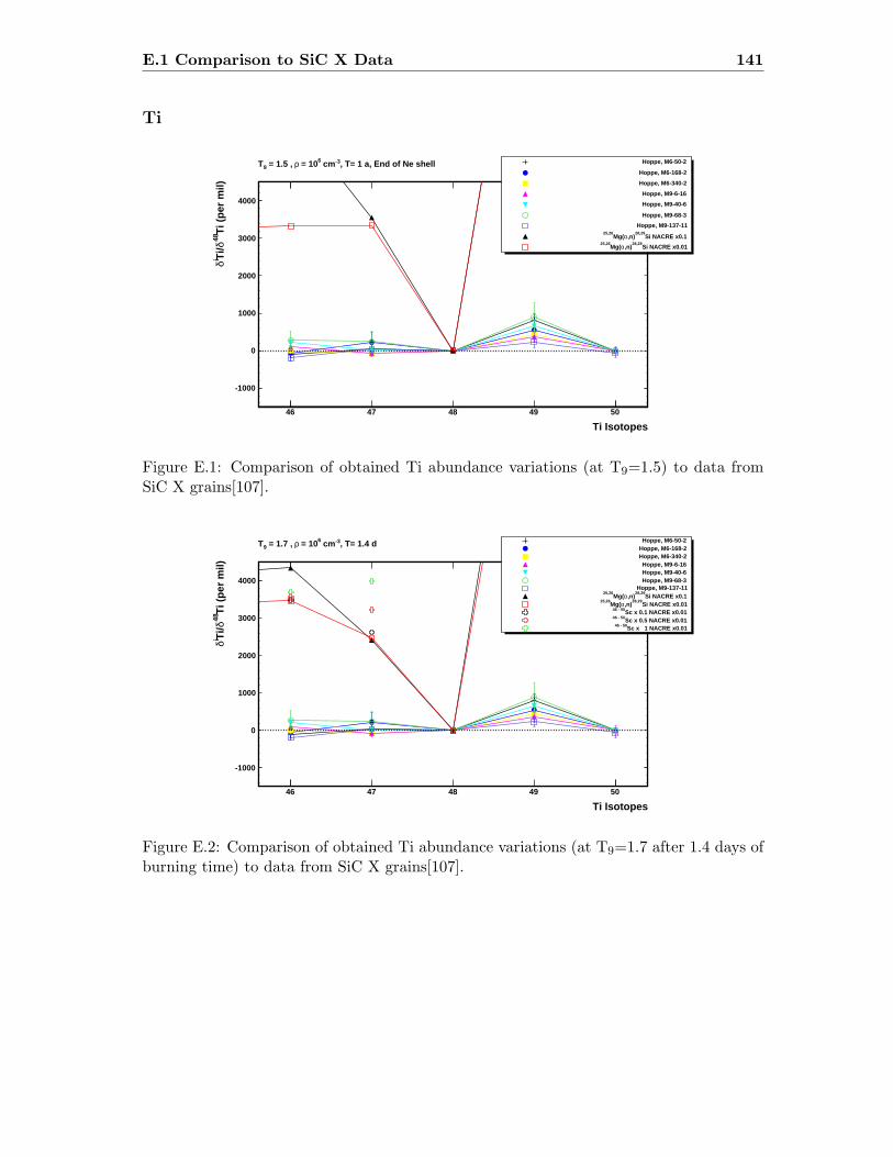
E.1 Comparison to SiC X Data 141
Ti
Ti Isotopes46 47 48 49 50
Ti (
per
mil)
48 dT
i/i d
-1000
0
1000
2000
3000
4000
Hoppe, M6-50-2
Hoppe, M6-168-2
Hoppe, M6-340-2
Hoppe, M9-6-16
Hoppe, M9-40-6
Hoppe, M9-68-3
Hoppe, M9-137-11
Si NACRE x0.128,29
,n)aMg(25,26
Si NACRE x0.0128,29
,n)aMg(25,26
, T= 1 a, End of Ne shell-3 cm6 = 10r = 1.5 , 9T
Figure E.1: Comparison of obtained Ti abundance variations (at T9=1.5) to data fromSiC X grains[107].
Ti Isotopes46 47 48 49 50
Ti (
per
mil)
48 dT
i/i d
-1000
0
1000
2000
3000
4000
Hoppe, M6-50-2Hoppe, M6-168-2Hoppe, M6-340-2Hoppe, M9-6-16Hoppe, M9-40-6Hoppe, M9-68-3
Hoppe, M9-137-11Si NACRE x0.1
28,29,n)aMg(
25,26
Si NACRE x0.0128,29
,n)aMg(25,26
Sc x 0.1 NACRE x0.0146 - 50
Sc x 0.5 NACRE x0.0146 - 50
Sc x 1 NACRE x0.0146 - 50
, T= 1.4 d-3 cm6 = 10r = 1.7 , 9T
Figure E.2: Comparison of obtained Ti abundance variations (at T9=1.7 after 1.4 days ofburning time) to data from SiC X grains[107].
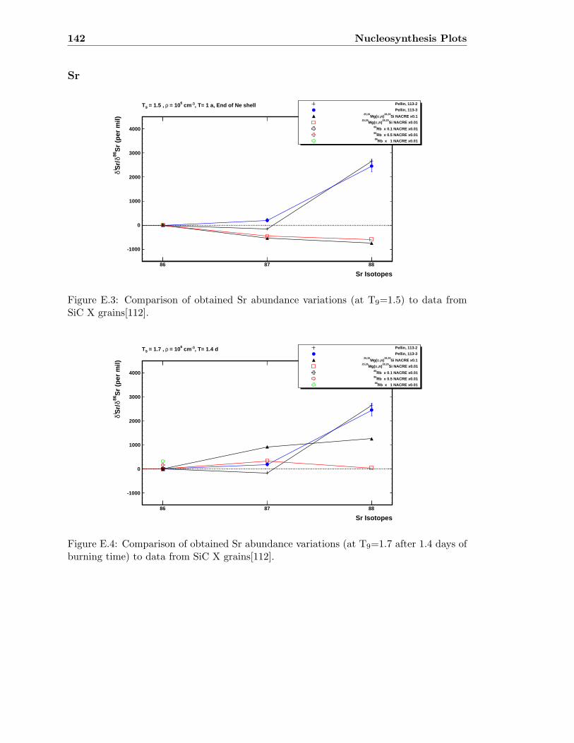
142 Nucleosynthesis Plots
Sr
Sr Isotopes86 87 88
Sr
(per
mil)
86 dS
r/i d
-1000
0
1000
2000
3000
4000
Pellin, 113-2
Pellin, 113-3
Si NACRE x0.128,29
,n)aMg(25,26
Si NACRE x0.0128,29
,n)aMg(25,26
Rb x 0.1 NACRE x0.0186
Rb x 0.5 NACRE x0.0186
Rb x 1 NACRE x0.0186
, T= 1 a, End of Ne shell-3 cm6 = 10r = 1.5 , 9T
Figure E.3: Comparison of obtained Sr abundance variations (at T9=1.5) to data fromSiC X grains[112].
Sr Isotopes86 87 88
Sr
(per
mil)
86 dS
r/i d
-1000
0
1000
2000
3000
4000
Pellin, 113-2
Pellin, 113-3
Si NACRE x0.128,29
,n)aMg(25,26
Si NACRE x0.0128,29
,n)aMg(25,26
Rb x 0.1 NACRE x0.0186
Rb x 0.5 NACRE x0.0186
Rb x 1 NACRE x0.0186
, T= 1.4 d-3 cm6 = 10r = 1.7 , 9T
Figure E.4: Comparison of obtained Sr abundance variations (at T9=1.7 after 1.4 days ofburning time) to data from SiC X grains[112].

E.1 Comparison to SiC X Data 143
Zr
Zr Isotopes90 91 92 93 94 95 96
Zr
(per
mil)
94 dZ
r/i d
-1000
0
1000
2000
3000
4000
5000
6000
7000
8000
Pellin, 113-2
Pellin, 113-3
Pellin, 196-5
Pellin, B2-05
Si NACRE x0.128,29
,n)aMg(25,26
Si NACRE x0.0128,29
,n)aMg(25,26
Sr x 0.1 NACRE x0.0190,91
Sr x 0.5 NACRE x0.0190,91
Sr x 1 NACRE x0.0190,91
, T= 1 a, End of Ne shell-3 cm6 = 10r = 1.5 , 9T
Figure E.5: Comparison of obtained Zr abundance variations (at T9=1.5) to data fromSiC X grains[112].
Zr Isotopes90 91 92 93 94 95 96
Zr
(per
mil)
94 dZ
r/i d
-1000
0
1000
2000
3000
4000
5000
6000
7000
8000
Pellin, 113-2
Pellin, 113-3
Pellin, 196-5
Pellin, B2-05
Si NACRE x0.128,29
,n)aMg(25,26
Si NACRE x0.0128,29
,n)aMg(25,26
Sr x 0.1 NACRE x0.0190,91
Sr x 0.5 NACRE x0.0190,91
Sr x 1 NACRE x0.0190,91
, T= 1.4 d-3 cm6 = 10r = 1.7 , 9T
Figure E.6: Comparison of obtained Zr abundance variations (at T9=1.7 after 1.4 days ofburning time) to data from SiC X grains[112].
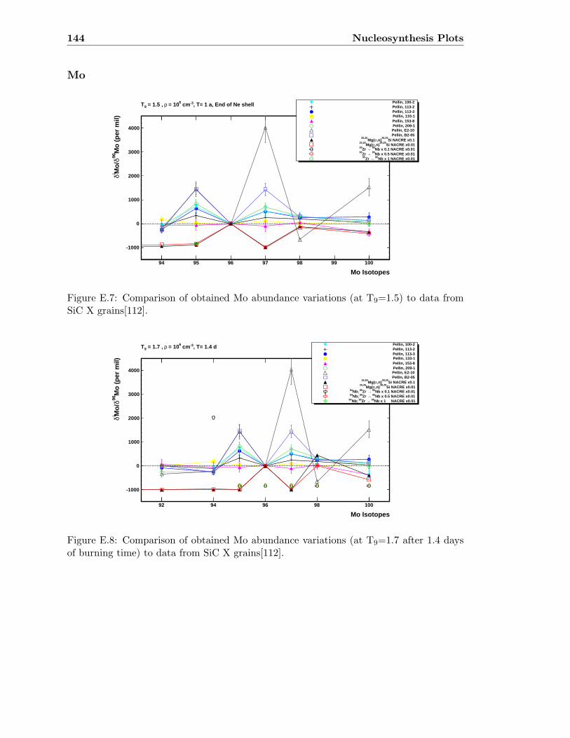
144 Nucleosynthesis Plots
Mo
Mo Isotopes94 95 96 97 98 99 100
Mo
(per
mil)
96 dM
o/i d
-1000
0
1000
2000
3000
4000
Pellin, 100-2Pellin, 113-2Pellin, 113-3Pellin, 133-1Pellin, 153-8Pellin, 209-1Pellin, E2-10Pellin, B2-05
Si NACRE x0.128,29
,n)aMg(25,26
Si NACRE x0.0128,29
,n)aMg(25,26
Nb x 0.1 NACRE x0.0195 ®Zr 95
Nb x 0.5 NACRE x0.0195 ®Zr 95
Nb x 1 NACRE x0.0195 ®Zr 95
, T= 1 a, End of Ne shell-3 cm6 = 10r = 1.5 , 9T
Figure E.7: Comparison of obtained Mo abundance variations (at T9=1.5) to data fromSiC X grains[112].
Mo Isotopes92 94 96 98 100
Mo
(per
mil)
96 dM
o/i d
-1000
0
1000
2000
3000
4000
Pellin, 100-2Pellin, 113-2Pellin, 113-3Pellin, 133-1Pellin, 153-8Pellin, 209-1Pellin, E2-10Pellin, B2-05
Si NACRE x0.128,29
,n)aMg(25,26
Si NACRE x0.0128,29
,n)aMg(25,26
Nb x 0.1 NACRE x0.0195 ®Zr 95Nb; 94
Nb x 0.5 NACRE x0.0195 ®Zr 95Nb; 94
Nb x 1 NACRE x0.0195 ®Zr 95Nb; 94
, T= 1.4 d-3 cm6 = 10r = 1.7 , 9T
Figure E.8: Comparison of obtained Mo abundance variations (at T9=1.7 after 1.4 daysof burning time) to data from SiC X grains[112].
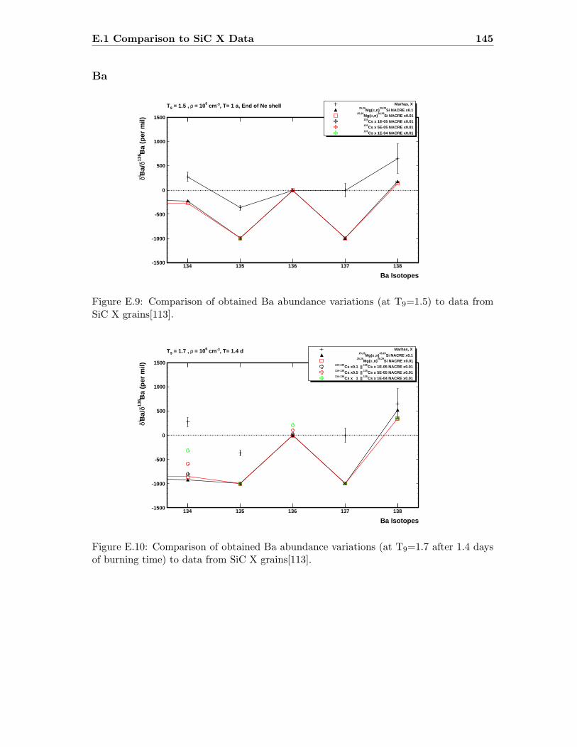
E.1 Comparison to SiC X Data 145
Ba
Ba Isotopes134 135 136 137 138
Ba
(per
mil)
136
dB
a/i d
-1500
-1000
-500
0
500
1000
1500
Marhas, X
Si NACRE x0.128,29
,n)aMg(25,26
Si NACRE x0.0128,29
,n)aMg(25,26
Cs x 1E-05 NACRE x0.01135
Cs x 5E-05 NACRE x0.01135
Cs x 1E-04 NACRE x0.01135
, T= 1 a, End of Ne shell-3 cm6 = 10r = 1.5 , 9T
Figure E.9: Comparison of obtained Ba abundance variations (at T9=1.5) to data fromSiC X grains[113].
Ba Isotopes134 135 136 137 138
Ba
(per
mil)
136
dB
a/i d
-1500
-1000
-500
0
500
1000
1500
Marhas, X
Si NACRE x0.128,29
,n)aMg(25,26
Si NACRE x0.0128,29
,n)aMg(25,26
Cs x 1E-05 NACRE x0.01135Cs x0.1 || 134-138
Cs x 5E-05 NACRE x0.01135Cs x0.5 || 134-138
Cs x 1E-04 NACRE x0.01135Cs x 1 || 134-138
, T= 1.4 d-3 cm6 = 10r = 1.7 , 9T
Figure E.10: Comparison of obtained Ba abundance variations (at T9=1.7 after 1.4 daysof burning time) to data from SiC X grains[113].

146 Nucleosynthesis Plots
E.2 Abundance Evolution
The abundance of specific isotopes as a function of time is plotted in the following figures.For the isotopes 25Mg and 26Mg the abundance evolution is plotted in each plot to allowa comparison to the reaction rates of 25Mg(α,n)28Si and 26Mg(α,n)29Si. Note, once anabundance reaches 10−13 the isotope is regarded as completely destroyed. The abundancevariations for T9 = 1.7 are shown for one year burning time, but are only interesting withrespect to nucleosynthesis for a burning time of 1.4 days.

E.2 Abundance Evolution 147
T9 = 1.5
Time [a]-210 -110 1
iX
-410
-310
-210
-110
1
= 1 a, End of Ne shell, NACRE x1max
, T-3 cm6= 10r = 1.5, 9T Mg25
Mg26
Si28
Si29
Si30
Figure E.11: Si abundance evolution at T9=1.5 for NACREx1.
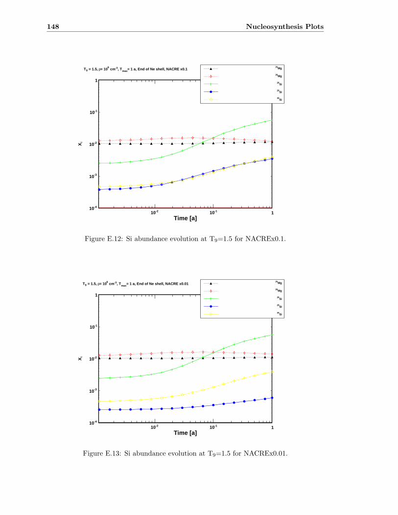
148 Nucleosynthesis Plots
Time [a]-210 -110 1
iX
-410
-310
-210
-110
1
= 1 a, End of Ne shell, NACRE x0.1max
, T-3 cm6= 10r = 1.5, 9T Mg25
Mg26
Si28
Si29
Si30
Figure E.12: Si abundance evolution at T9=1.5 for NACREx0.1.
Time [a]-210 -110 1
iX
-410
-310
-210
-110
1
= 1 a, End of Ne shell, NACRE x0.01max
, T-3 cm6= 10r = 1.5, 9T Mg25
Mg26
Si28
Si29
Si30
Figure E.13: Si abundance evolution at T9=1.5 for NACREx0.01.
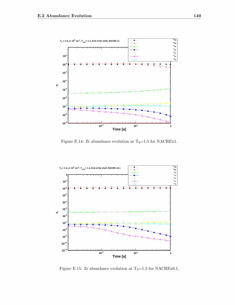
E.2 Abundance Evolution 149
Time [a]-210 -110 1
iX
-910
-810
-710
-610
-510
-410
-310
-210
-110
= 1 a, End of Ne shell, NACRE x1max
, T-3 cm6= 10r = 1.5, 9T Mg25
Mg26
Sr88
Zr93
Zr94
Zr95
Zr96
Figure E.14: Zr abundance evolution at T9=1.5 for NACREx1.
Time [a]-210 -110 1
iX
-1110
-1010
-910
-810
-710
-610
-510
-410
-310
-210
-110
1
= 1 a, End of Ne shell, NACRE x0.1max
, T-3 cm6= 10r = 1.5, 9TMg25
Mg26
Sr88
Zr93
Zr94
Zr95
Zr96
Figure E.15: Zr abundance evolution at T9=1.5 for NACREx0.1.
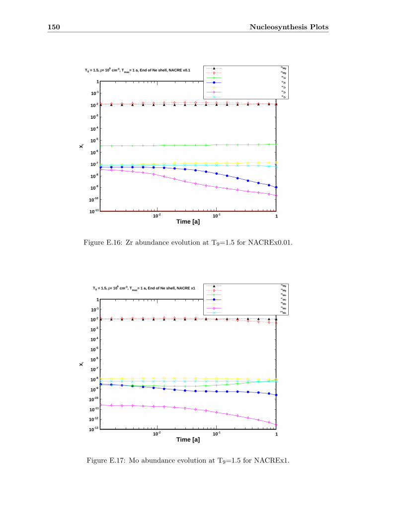
150 Nucleosynthesis Plots
Time [a]-210 -110 1
iX
-1110
-1010
-910
-810
-710
-610
-510
-410
-310
-210
-110
1
= 1 a, End of Ne shell, NACRE x0.1max
, T-3 cm6= 10r = 1.5, 9TMg25
Mg26
Sr88
Zr93
Zr94
Zr95
Zr96
Figure E.16: Zr abundance evolution at T9=1.5 for NACREx0.01.
Time [a]-210 -110 1
iX
-1310
-1210
-1110
-1010
-910
-810
-710
-610
-510
-410
-310
-210
-110
1
= 1 a, End of Ne shell, NACRE x1max
, T-3 cm6= 10r = 1.5, 9TMg25
Mg26
Mo96
Mo97
Mo98
Mo99
Mo100
Figure E.17: Mo abundance evolution at T9=1.5 for NACREx1.
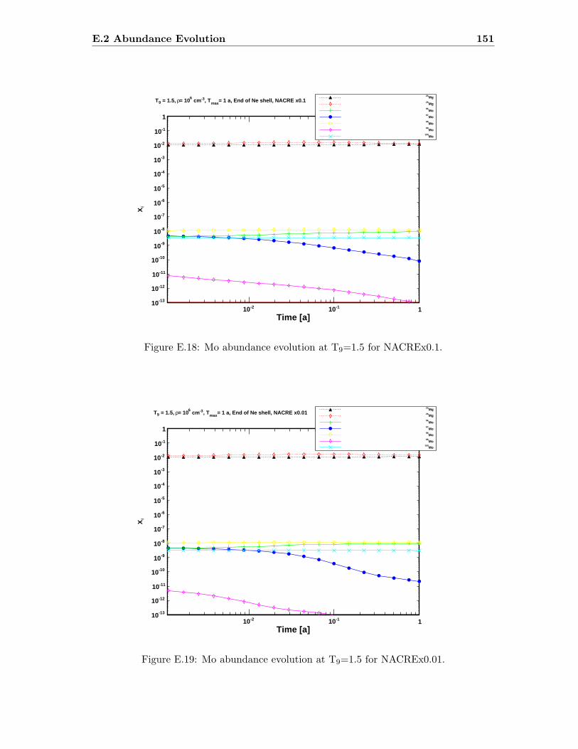
E.2 Abundance Evolution 151
Time [a]-210 -110 1
iX
-1310
-1210
-1110
-1010
-910
-810
-710
-610
-510
-410
-310
-210
-110
1
= 1 a, End of Ne shell, NACRE x0.1max
, T-3 cm6= 10r = 1.5, 9TMg25
Mg26
Mo96
Mo97
Mo98
Mo99
Mo100
Figure E.18: Mo abundance evolution at T9=1.5 for NACREx0.1.
Time [a]-210 -110 1
iX
-1310
-1210
-1110
-1010
-910
-810
-710
-610
-510
-410
-310
-210
-110
1
= 1 a, End of Ne shell, NACRE x0.01max
, T-3 cm6= 10r = 1.5, 9TMg25
Mg26
Mo96
Mo97
Mo98
Mo99
Mo100
Figure E.19: Mo abundance evolution at T9=1.5 for NACREx0.01.
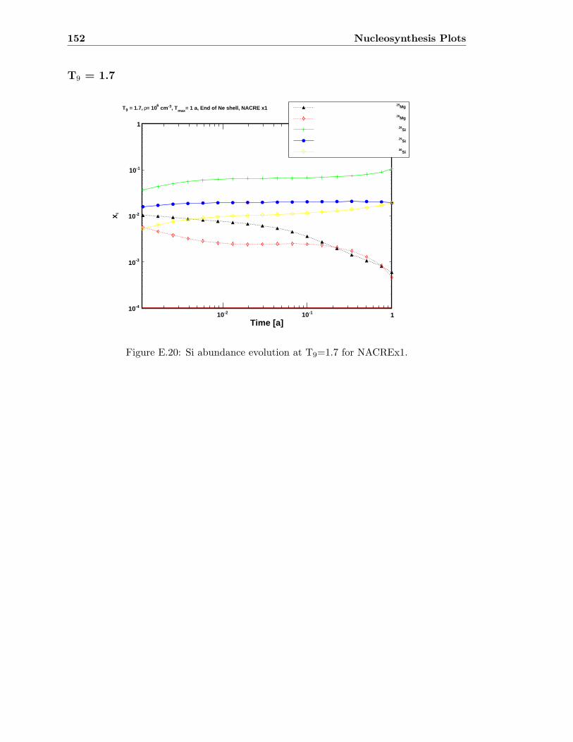
152 Nucleosynthesis Plots
T9 = 1.7
Time [a]-210 -110 1
iX
-410
-310
-210
-110
1
= 1 a, End of Ne shell, NACRE x1max
, T-3 cm6= 10r = 1.7, 9T Mg25
Mg26
Si28
Si29
Si30
Figure E.20: Si abundance evolution at T9=1.7 for NACREx1.
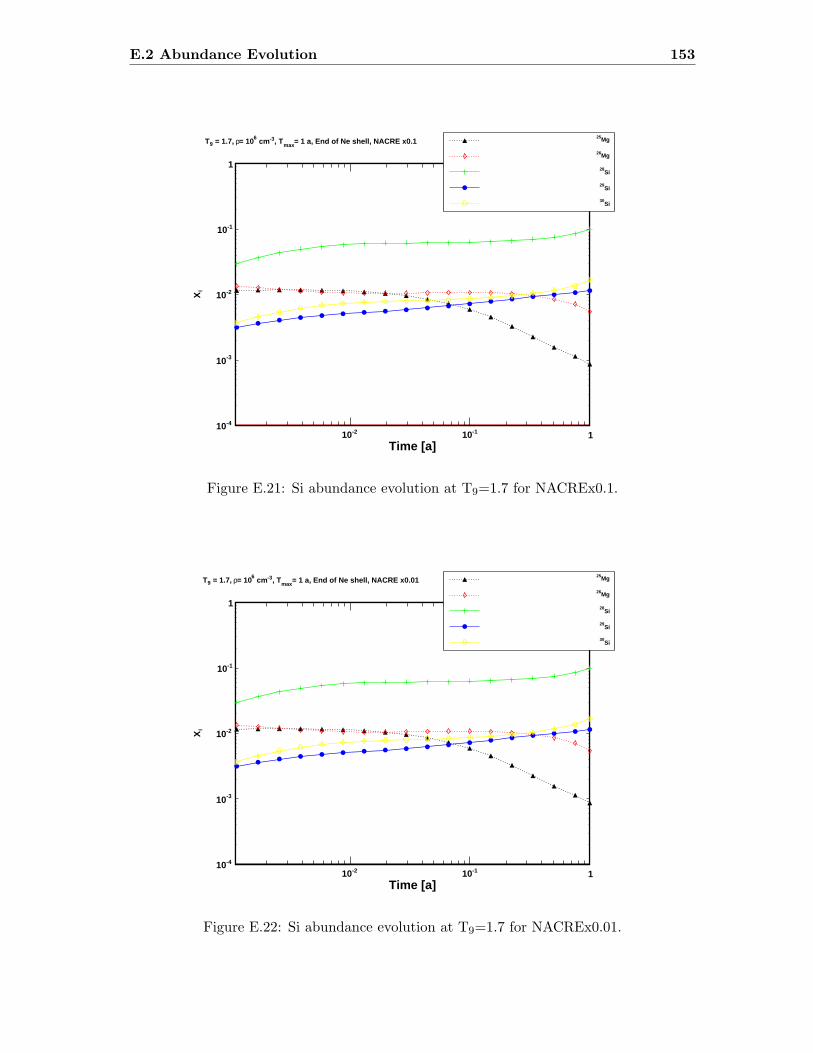
E.2 Abundance Evolution 153
Time [a]-210 -110 1
iX
-410
-310
-210
-110
1
= 1 a, End of Ne shell, NACRE x0.1max
, T-3 cm6= 10r = 1.7, 9T Mg25
Mg26
Si28
Si29
Si30
Figure E.21: Si abundance evolution at T9=1.7 for NACREx0.1.
Time [a]-210 -110 1
iX
-410
-310
-210
-110
1
= 1 a, End of Ne shell, NACRE x0.01max
, T-3 cm6= 10r = 1.7, 9T Mg25
Mg26
Si28
Si29
Si30
Figure E.22: Si abundance evolution at T9=1.7 for NACREx0.01.
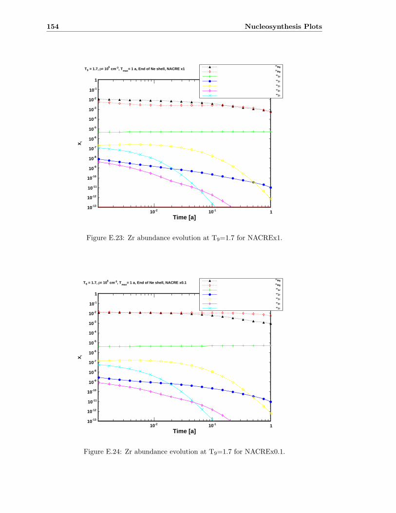
154 Nucleosynthesis Plots
Time [a]-210 -110 1
iX
-1310
-1210
-1110
-1010
-910
-810
-710
-610
-510
-410
-310
-210
-110
1
= 1 a, End of Ne shell, NACRE x1max
, T-3 cm6= 10r = 1.7, 9TMg25
Mg26
Sr88
Zr93
Zr94
Zr95
Zr96
Figure E.23: Zr abundance evolution at T9=1.7 for NACREx1.
Time [a]-210 -110 1
iX
-1310
-1210
-1110
-1010
-910
-810
-710
-610
-510
-410
-310
-210
-110
1
= 1 a, End of Ne shell, NACRE x0.1max
, T-3 cm6= 10r = 1.7, 9TMg25
Mg26
Sr88
Zr93
Zr94
Zr95
Zr96
Figure E.24: Zr abundance evolution at T9=1.7 for NACREx0.1.
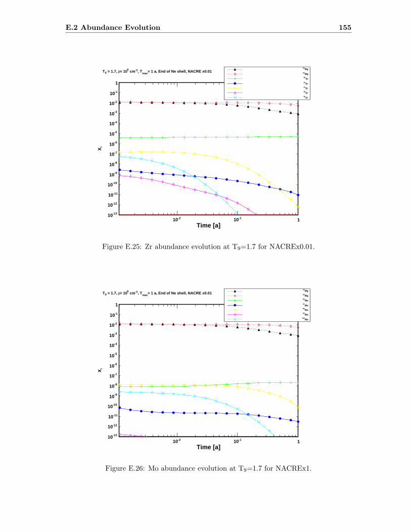
E.2 Abundance Evolution 155
Time [a]-210 -110 1
iX
-1310
-1210
-1110
-1010
-910
-810
-710
-610
-510
-410
-310
-210
-110
1
= 1 a, End of Ne shell, NACRE x0.01max
, T-3 cm6= 10r = 1.7, 9TMg25
Mg26
Sr88
Zr93
Zr94
Zr95
Zr96
Figure E.25: Zr abundance evolution at T9=1.7 for NACREx0.01.
Time [a]-210 -110 1
iX
-1310
-1210
-1110
-1010
-910
-810
-710
-610
-510
-410
-310
-210
-110
1
= 1 a, End of Ne shell, NACRE x0.01max
, T-3 cm6= 10r = 1.7, 9TMg25
Mg26
Mo96
Mo97
Mo98
Mo99
Mo100
Figure E.26: Mo abundance evolution at T9=1.7 for NACREx1.
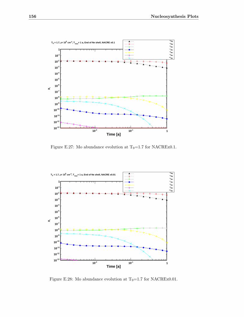
156 Nucleosynthesis Plots
Time [a]-210 -110 1
iX
-1310
-1210
-1110
-1010
-910
-810
-710
-610
-510
-410
-310
-210
-110
1
= 1 a, End of Ne shell, NACRE x0.1max
, T-3 cm6= 10r = 1.7, 9TMg25
Mg26
Mo96
Mo97
Mo98
Mo99
Mo100
Figure E.27: Mo abundance evolution at T9=1.7 for NACREx0.1.
Time [a]-210 -110 1
iX
-1310
-1210
-1110
-1010
-910
-810
-710
-610
-510
-410
-310
-210
-110
1
= 1 a, End of Ne shell, NACRE x0.01max
, T-3 cm6= 10r = 1.7, 9TMg25
Mg26
Mo96
Mo97
Mo98
Mo99
Mo100
Figure E.28: Mo abundance evolution at T9=1.7 for NACREx0.01.

Bibliography
[1] A. S. Eddington. The Internal Constitution of the Stars. Science, 52:233–240, 1920.
[2] E. M. Burbidge et al. Synthesis of the Elements in Stars. Rev. Mod. Phys., 29:547–650, 1957.
[3] A. G. W. Cameron. Origin of Anomalous Abundances of the Elements in GiantStars. Astrophysical Journal, 121:144, 1955.
[4] W. A. Fowler et al. Stellar Evolution and the Synthesis of the Elements. Astrophys-ical Journal, 122:271, 1955.
[5] R. Hirschi et al. NuGrid: S Process in Massive Stars. In Nuclei in the Cosmos (NICX), 2008.
[6] R. D. Hoffman et al. Nucleosynthesis below A = 100 in Massive Stars. The Astro-physical Journal, 549:1085–1092, 2001.
[7] M. Pignatari. The Weak S-Process in Massive Stars. PhD thesis, Universita DegliStudi Di Torino, 2006.
[8] A. Denker. Drei Neutronenerzeugungsreaktionen in Sternen. PhD thesis, Universityof Stuttgart, 1994.
[9] F. Herwig. Evolution of Asymptotic Giant Branch Stars. Annual Review of Astron-omy and Astrophysics, 43:435–479, 2005.
[10] S. E. Woosley et al. The Evolution and Explosion of Massive Stars. Rev. Mod.Phys., 74:1015–1071, 2002.
[11] M. Arnould and S. Goriely. The P-Process of Stellar Nucleosynthesis: Astrophysicsand Nuclear Physics Status. Physics Reports, 384:1–84, 2003.
[12] C. Frohlich et al. Neutrino-Induced Nucleosynthesis of A > 64 Nuclei: The νpProcess. Physical Review Letters, 96:142502, 2006.
[13] D. D. Clayton. Principles of Stellar Evolution and Nucleosynthesis. The Universityof Chicago Press, 1968.
[14] D. D. Clayton et al. Neutron Capture Chains in Heavy Element Synthesis. Annalsof Physics, 12:331 – 408, 1961.
[15] P. A. Seeger et al. Nucleosynthesis of Heavy Elements by Neutron Capture. Astro-physical Journal Supplement Series, 11:121, 1965.
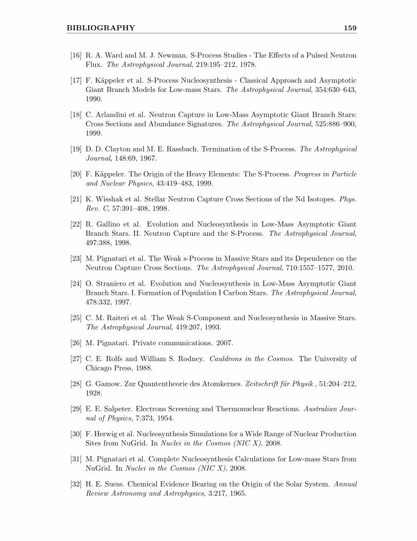
BIBLIOGRAPHY 159
[16] R. A. Ward and M. J. Newman. S-Process Studies - The Effects of a Pulsed NeutronFlux. The Astrophysical Journal, 219:195–212, 1978.
[17] F. Kappeler et al. S-Process Nucleosynthesis - Classical Approach and AsymptoticGiant Branch Models for Low-mass Stars. The Astrophysical Journal, 354:630–643,1990.
[18] C. Arlandini et al. Neutron Capture in Low-Mass Asymptotic Giant Branch Stars:Cross Sections and Abundance Signatures. The Astrophysical Journal, 525:886–900,1999.
[19] D. D. Clayton and M. E. Rassbach. Termination of the S-Process. The AstrophysicalJournal, 148:69, 1967.
[20] F. Kappeler. The Origin of the Heavy Elements: The S-Process. Progress in Particleand Nuclear Physics, 43:419–483, 1999.
[21] K. Wisshak et al. Stellar Neutron Capture Cross Sections of the Nd Isotopes. Phys.Rev. C, 57:391–408, 1998.
[22] R. Gallino et al. Evolution and Nucleosynthesis in Low-Mass Asymptotic GiantBranch Stars. II. Neutron Capture and the S-Process. The Astrophysical Journal,497:388, 1998.
[23] M. Pignatari et al. The Weak s-Process in Massive Stars and its Dependence on theNeutron Capture Cross Sections. The Astrophysical Journal, 710:1557–1577, 2010.
[24] O. Straniero et al. Evolution and Nucleosynthesis in Low-Mass Asymptotic GiantBranch Stars. I. Formation of Population I Carbon Stars. The Astrophysical Journal,478:332, 1997.
[25] C. M. Raiteri et al. The Weak S-Component and Nucleosynthesis in Massive Stars.The Astrophysical Journal, 419:207, 1993.
[26] M. Pignatari. Private communications. 2007.
[27] C. E. Rolfs and William S. Rodney. Cauldrons in the Cosmos. The University ofChicago Press, 1988.
[28] G. Gamow. Zur Quantentheorie des Atomkernes. Zeitschrift fur Physik , 51:204–212,1928.
[29] E. E. Salpeter. Electrons Screening and Thermonuclear Reactions. Australian Jour-nal of Physics, 7:373, 1954.
[30] F. Herwig et al. Nucleosynthesis Simulations for a Wide Range of Nuclear ProductionSites from NuGrid. In Nuclei in the Cosmos (NIC X), 2008.
[31] M. Pignatari et al. Complete Nucleosynthesis Calculations for Low-mass Stars fromNuGrid. In Nuclei in the Cosmos (NIC X), 2008.
[32] H. E. Suess. Chemical Evidence Bearing on the Origin of the Solar System. AnnualReview Astronomy and Astrophysics, 3:217, 1965.

160 BIBLIOGRAPHY
[33] A. G. W. Cameron. The Formation of the Sun and Planets. Icarus, 1:13–69, 1962.
[34] U. Ott. Interstellar grains in meteorites. Nature, 364:25–33, 1993.
[35] E. K. Zinner. Presolar Grains. Treatise on Geochemistry, 1:17–39, 2003.
[36] J. K. Bair and H. B. Willard. Level Structure in 22Ne and 30Si from the Reactions18O(α, n)21Ne and 26Mg(α,n)29Si. Phys. Rev., 128:299–304, 1962.
[37] J. P. Russell et al. Levels in 30Si Excited by the 26Mg(α,n)29Si, 26Mg(α,γ)30Si and26Mg(α,α)26Mg Reactions. Nuclear Physics A, 187:449 – 458, 1972.
[38] L. V. Namjoshi et al. Resonance Spectroscopy of the 30Si Nucleus in the ExcitationEnergy Range 14.27 to 15.02 MeV. Phys. Rev. C, 13:915–921, 1976.
[39] O. Bassey Okon II. Investigations in Radiative Alpha Capture in 29Si,26Mg,35P,35Cland 37Cl . PhD thesis, State University of New York at Albany, 1973.
[40] L. Van der Zwan and K. W. Geiger. Cross Sections for the 25Mg(α,n)28Si Reactionat Eα < 4.8 MeV. Nucl. Sci. Eng., 79:197–201, 1981.
[41] W. M. Howard et al. Nucleosynthesis of Rare Nuclei from Seed Nuclei in ExplosiveCarbon Burning. The Astrophysical Journal, 175:201, 1972.
[42] M. R. Anderson et al. 25Mg(α,n)28Si and 26Mg(α,n)29Si as Neutron Sources inExplosive Neon Burning. Nuclear Physics A, 405:170 – 178, 1983.
[43] S. Kuchler. Untersuchung der Reaktionen 25Mg(α,n)28Si und 26Mg(α,n)29Si. Mas-ter’s thesis, University of Stuttgart, 1990.
[44] J. K. Bair and F. X. Haas. Total Neutron Yield from the Reactions 13C(α,n)16Oand 17,18O(α, n)21Ne. Phys. Rev. C, 7:1356–1364, 1973.
[45] O. Wieland. Untersuchung der Reaktionen 25Mg(α,n)28Si und 26Mg(α,n)29Si. Mas-ter’s thesis, University of Stuttgart, 1995.
[46] R. Crowter. Master’s thesis. Master’s thesis, University of Surrey, 2007.
[47] S. E. Woosley et al. Semiempirical Thermonuclear Reaction-Rate Data forIntermediate-Mass Nuclei. Atomic Data and Nuclear Data Tables, 22:371 – 441,1978.
[48] G. R. Caughlan and W. A. Fowler. Thermonuclear Reaction Rates V. Atomic Dataand Nuclear Data Tables, 40:283, 1988.
[49] L. E. Brown and D. D. Clayton. SiC Particles from Asymptotic Giant Branch Stars- Mg Burning and the S-Process. Astrophysical Journal Letters, 392:L79–L82, 1992.
[50] P. Hoppe et al. Carbon, Nitrogen, Magnesium, Silicon and Titanium Isotopic Com-positions of Single Interstellar Silicon Carbide Grains from the Murchison Carbona-ceous Chondrite. The Astrophysical Journal, 430:870–890, 1994.
[51] E. Zinner et al. Silicon and Carbon Isotopic Ratios in AGB Stars: SiC Grain Data,Models, and the Galactic Evolution of the Si Isotopes. The Astrophysical Journal,650:350–373, 2006.

BIBLIOGRAPHY 161
[52] S. Mostefaoui and P. Hoppe. Discovery of Abundant In Situ Silicate and SpinelGrains from Red Giant Stars in a Primitive Meteorite. The Astrophysical JournalLetters, 613:L149–L152, 2004.
[53] M. Lugaro et al. Si Isotopic Ratios in Mainstream Presolar SiC Grains Revisited.The Astrophysical Journal, 527:369–394, 1999.
[54] P. Hoppe et al. An Unusual Presolar Silicon Carbide Grain From a Supernova :Implications for the Production of 29Si in Type II Supernovae. The AstrophysicalJournal Letters, 691, 2009.
[55] T. Rauscher et al. Nucleosynthesis in Massive Stars with Improved Nuclear andStellar Physics. The Astrophysical Journal, 576:L20–L23, 2002.
[56] W. A. Fowler et al. Thermonuclear Reaction Rates II. Annual Review of Astronomyand Astrophysics, 13:69, 1975.
[57] C. Angulo et al. A Compilation of Charged-Particle Induced Thermonuclear Reac-tion Rates. Nuclear Physics A, 656:3 – 183, 1999.
[58] S. Dababneh et al. Stellar He Burning of 18O : A Measurement of Low-EnergyResonances and their Astrophysical Implications. Phys. Rev. C, 68:025801, 2003.
[59] R. S. Lewis et al. Interstellar Grains in Meteorites: II. SiC and its Noble Gases.Geochimica et Cosmochimica Acta, 58:471 – 494, 1994.
[60] P. R. Heck et al. Interstellar Residence Times of Presolar SiC Dust Grains fromthe Murchison Carbonaceous Meteorite. The Astrophysical Journal, 698:1155–1164,2009.
[61] J. C. Overley et al. The Energy Calibration of Tandem Accelerators. NuclearInstruments and Methods, 68:61 – 69, 1969.
[62] C. H. Johnson et al. Thresholds for (p,n) Reactions on 26 Intermediate-WeightNuclei. Phys. Rev., 136:B1719–B1729, 1964.
[63] National Nuclear Data Center. Evaluated Nuclear Data Files - ENDF and JENDL.http://www.nndc.bnl.gov/exfor/endf00.jsp.
[64] A. O. Hanson and J. L. McKibben. A Neutron Detector Having Uniform Sensitivityfrom 10 keV to 3 MeV. Phys. Rev., 72:673–677, 1947.
[65] L.V. East and R.B. Walton. Polyethylene Moderated 3He Neutron Detectors. Nu-clear Instruments and Methods, 72:161 – 166, 1969.
[66] B. Holmqvist and E. Ramstrom. A High Efficiency 4π Neutron Detector. NuclearInstruments and Methods in Physics Research, 188:153 – 157, 1981.
[67] L. B. Borst. Low-Temperature Neutron Moderation. Phys. Rev. Lett., 4:131, 1960.
[68] K. Wolke. Helium burning of 22Ne. Zeitschrift fur Physik A Hadrons and Nuclei,334:491–510, 1989.
[69] V. Harms et al. Properties of 22Ne(α,n)25Mg resonances. Phys. Rev. C, 43:2849–2861, 1991.
162 BIBLIOGRAPHY
[70] H. W. Drotleff. Untersuchung der S-Prozess Neutronenquelle 22Ne(α, n)25Mg. PhDthesis, Ruhr-Universitat Bochum, 1992.
[71] M. Jager. Die Einfangreaktion 22Ne(α,n)25Mg -die Hauptneutronenquelle in Mas-siven Sternen. PhD thesis, Universitat Stuttgart, 2001.
[72] S. Agostinelli et al. GEANT4 – a Simulation Toolkit. Nuclear Instruments andMethods in Physics Research Section A: Accelerators, Spectrometers, Detectors andAssociated Equipment, 506:250–303, 2003.
[73] Los Alamos National Laboratory. MCNP - A General Monte Carlo N-Particle Trans-port Code - Version 5. http://mcnp-green.lanl.gov/index.html.
[74] GEANT4 - User Documentation and Forum. http://geant4.web.cern.ch/geant4/support/.
[75] T. Koi. GEANT4 - Thermal Neutron Scattering in GEANT4.http://geant4hadronics.wikispaces.com/Thermal+Neutron+Scattering+in+Geant4.
[76] The Root Team CERN. ROOT - An Object Oriented Data Analysis Framework.http://root.cern.ch/.
[77] J. L. Zyskind et al. Competition effects in proton-induced reactions on 51V. NuclearPhysics A, 343:295 – 314, 1980.
[78] K. K. Harris et al. The 51V(p,n)51Cr reaction as a neutron source of known intensity.Nuclear Instruments and Methods, 33:257 – 260, 1965.
[79] M. Heil et al. The 13C(α,n) Reaction and its Role as a Neutron Source for the sProcess. Physical Review C (Nuclear Physics), 78:025803, 2008.
[80] M. Heagney. Reduction Techniques for Isotopic Materials. International NuclearTarget Development Society, Los Alamos National Laboratory, 1976.
[81] S. Takayanagi et al. On the Preparation of Magnesium Targets from MgO. NuclearInstruments and Methods, 45:345 – 346, 1966.
[82] S.H. Maxman. Target Preparation Techniques. Nuclear Instruments and Methods,50(1):53 – 60, 1967.
[83] R. B. Weinberg et al. Deuteron Stripping Reaction on 25Mg. Phys. Rev., 133:B884–B892, 1964.
[84] A. H. F. Muggleton. Preparation of Thin Nuclear Targets. Journal of Physics E:Scientific Instruments, 12:780, 1979.
[85] G. M. Hinn et al. Production of Thick Elemental Low-Oxygen Content nat,26Mgfrom nat,26MgO. Nuclear Instruments and Methods in Physics Research Section A:Accelerators, Spectrometers, Detectors and Associated Equipment, 227:434 – 436,1984.
[86] D.A Vermilyea. The formation of anodic oxide films on tantalum in non-aqueoussolutions. Acta Metallurgica, 2:482 – 486, 1954.
[87] A. Best. unpublished results. 2009.
BIBLIOGRAPHY 163
[88] A. Best. to be published. PhD thesis, University of Notre Dame.
[89] E. Strandberg et al. 24Mg(α,γ)28Si Resonance Parameters at Low Alpha-ParticleEnergies. Physical Review C (Nuclear Physics), 77:055801, 2008.
[90] C. E. Aalseth et al. Ultra-Low-Background Copper Production and Clean Fabrica-tion. volume 785, pages 170–176. AIP, 2005.
[91] E.W. Hoppe et al. Cleaning and Passivation of Copper Surfaces to Remove SurfaceRadioactivity and Prevent Oxide Formation. Nuclear Instruments and Methods inPhysics Research Section A: Accelerators, Spectrometers, Detectors and AssociatedEquipment, 579:486 – 489, 2007. Proceedings of the 11th Symposium on RadiationMeasurements and Applications.
[92] H.Y. Lee. The 18F(α,p)21Ne Reaction and Its Astrophysical Implications. PhDthesis, University of Notre Dame du Lac, 2006.
[93] J.F. Ziegler et al. The Stopping and Range of Ions in Solids. Pergamon Press, 1985.
[94] X. Xu et al. Interfacial Reactions between Oxide Films and Refractory Metal Sub-strates. Langmuir, 12:4877?4881, 1996.
[95] Albert E. Evans Jr. Energy dependence of the response of a 3He long counter.Nuclear Instruments and Methods in Physics Research, 199:643 – 644, 1982.
[96] K. K. Sekharan et al. A Neutron Detector for Measurement of Total Neutron Pro-duction Cross Sections. Nuclear Instruments and Methods, 133:253 – 257, 1976.
[97] P. Hosmer. Beta-Decay Studies of 78Ni and Other Neutron-Rich Nuclei in the As-trophysical R-Process. PhD thesis, Michigan State University, 2005.
[98] S. Harissopulos et al. Cross Section of the 13C(α,n)16O Reaction: A Background forthe Measurement of Geo-Neutrinos. Phys. Rev. C, 72:062801, 2005.
[99] M. Kurth. The Initial Oxidation Of Magnesium. PhD thesis, Universitat Stuttgart,2004.
[100] E. Raub et al. Inkorporation kohlenstoffhaltiger Fremdstoffe bei der galvanischenAbscheidung von Gold- und Goldlegierungsuberzugen in sauren und alkalischenCyanidbadern. Materials and Corrosion/Werkstoffe und Korrosion, 23:643–647,1972.
[101] T. R. Wang et al. 11B+α Reaction Rates and Primordial Nucleosynthesis. Phys.Rev. C, 43:883–896, Feb 1991.
[102] P. M. Endt. Energy Levels of A = 21-44 Nuclei (VII). Nuclear Physics A, 521, 1990.
[103] P. M. Endt. Supplement to Energy Levels of A = 21-44 Nuclei (VII). NuclearPhysics A, 633:1 – 220, 1998.
[104] R.B. Firestone. Nuclear Data Sheets for A = 22. Nuclear Data Sheets, 106:1 – 88,2005.
[105] T. Rauscher et al. Astrophysical Reaction Rates From Statistical Model Calcula-tions. Atomic Data and Nuclear Data Tables, 75:1 – 351, 2000.

[106] S. W. J. Colgan et al. Day 640 infrared line and continuum measurements: Dustformation in SN 1987A. The Astrophysical Journal, 427:874–888, 1994.
[107] P. Hoppe and A. Besmehn. Evidence for Extinct Vanadium-49 in Presolar SiliconCarbide Grains from Supernovae. The Astrophysical Journal Letters, 576:L69–L72,September 2002.
[108] S. Amari, P. Hoppe, E. Zinner, and R. S. Lewis. Trace-element concentrations insingle circumstellar silicon carbide grains from the Murchison meteorite. Meteoritics,30:679, 1995.
[109] K. Lodders and B. Fegley, Jr. The origin of circumstellar silicon carbide grains foundin meteorites. Meteoritics, 30:661, November 1995.
[110] J. Spyromilio, R. A. Stathakis, and G. R. Meurer. Clumping and Smallscale Mixingin Supernova 1987A. Monthly Notices of the Royal Astronomical Society, 263:530,1993.
[111] E. Anders and N. Grevesse. Abundances of the Elements: Meteoritic and Solar.Geochimica et Cosmochimica Acta, 53:197 – 214, 1989.
[112] M. J. Pellin et al. Heavy Metal Isotopic Anomalies in Supernovae Presolar Grains.In 37th Annual Lunar and Planetary Science Conference, volume 37, page 2041,2006.
[113] K. K. Marhas et al. NanoSIMS studies of Ba isotopic compositions in single presolarsilicon carbide grains from AGB stars and supernovae. Meteoritics and PlanetaryScience, 42:1077–1101, 2007.
[114] B. S. Meyer et al. Molybdenum and Zirconium Isotopes from a Supernova NeutronBurst. The Astrophysical Journal Letters, 540:L49–L52, 2000.
[115] A. I. Karakas et al. The Impact of the 18F(α,p)21Ne Reaction on Asymptotic GiantBranch Nucleosynthesis. The Astrophysical Journal, 676:1254–1261, 2008.
[116] M. Pignatari et al. in preparation. 2010.
[117] M. Tode et al. Removal of Carbon Contamination on Si Wafers with an ExcimerLamp. Metallurgical and Materials Transactions A, 38:596–598, 2007.
[118] D. C. Powell et al. Low-Energy Resonance Strengths for Proton Capture on Mg andAl Nuclei. Nuclear Physics A, 644:263 – 276, 1998.