Expanding the applicability of Inexact Newton Methods under Smale’s (α, γ)-theory
14
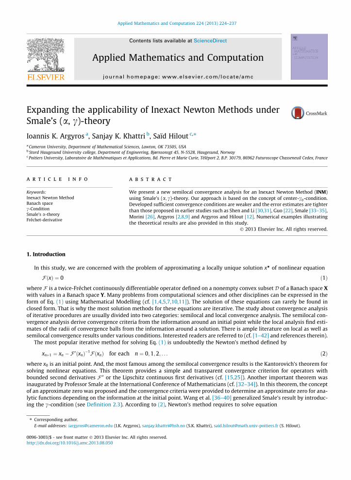
Expanding the applicability of Inexact Newton Methods under Smale’s (a, c)-theory Ioannis K. Argyros a , Sanjay K. Khattri b , Saïd Hilout c,⇑ a Cameron University, Department of Mathematical Sciences, Lawton, OK 73505, USA b Stord Haugesund University college, Department of Engineering, Bjørnsonsgt 45, N-5528, Haugesund, Norway c Poitiers University, Laboratoire de Mathématiques et Applications, Bd. Pierre et Marie Curie, Téléport 2, B.P. 30179, 86962 Futuroscope Chasseneuil Cedex, France article info Keywords: Inexact Newton Method Banach space c-Condition Smale’s a-theory Fréchet-derivative abstract We present a new semilocal convergence analysis for an Inexact Newton Method (INM) using Smale’s (a; c)-theory. Our approach is based on the concept of center-c 0 -condition. Developed sufficient convergence conditions are weaker and the error estimates are tighter than those proposed in earlier studies such as Shen and Li [30,31], Guo [22], Smale [33–35], Morini [26], Argyros [2,8,9] and Argyros and Hilout [12]. Numerical examples illustrating the theoretical results are also provided in this study. Ó 2013 Elsevier Inc. All rights reserved. 1. Introduction In this study, we are concerned with the problem of approximating a locally unique solution x H of nonlinear equation FðxÞ¼ 0 ð1Þ where F is a twice-Fréchet continuously differentiable operator defined on a nonempty convex subset D of a Banach space X with values in a Banach space Y. Many problems from computational sciences and other disciplines can be expressed in the form of Eq. (1) using Mathematical Modelling (cf. [1,4,5,7,10,11]). The solution of these equations can rarely be found in closed form. That is why the most solution methods for these equations are iterative. The study about convergence analysis of iterative procedures are usually divided into two categories: semilocal and local convergence analysis. The semilocal con- vergence analysis derive convergence criteria from the information around an initial point while the local analysis find esti- mates of the radii of convergence balls from the information around a solution. There is ample literature on local as well as semilocal convergence results under various conditions. Interested readers are referred to (cf. [1–42] and references therein). The most popular iterative method for solving Eq. (1) is undoubtedly the Newton’s method defined by x nþ1 ¼ x n F 0 ðx n Þ 1 Fðx n Þ for each n ¼ 0; 1; 2; ... ð2Þ where x 0 is an initial point. And, the most famous among the semilocal convergence results is the Kantorovich’s theorem for solving nonlinear equations. This theorem provides a simple and transparent convergence criterion for operators with bounded second derivatives F 00 or the Lipschitz continuous first derivatives (cf. [15,25]). Another important theorem was inaugurated by Professor Smale at the International Conference of Mathematicians (cf. [32–34]). In this theorem, the concept of an approximate zero was proposed and the convergence criteria were provided to determine an approximate zero for ana- lytic functions depending on the information at the initial point. Wang et al. [36–40] generalized Smale’s result by introduc- ing the c-condition (see Definition 2.3). According to (2), Newton’s method requires to solve equation 0096-3003/$ - see front matter Ó 2013 Elsevier Inc. All rights reserved. http://dx.doi.org/10.1016/j.amc.2013.08.050 ⇑ Corresponding author. E-mail addresses: [email protected] (I.K. Argyros), [email protected] (S.K. Khattri), [email protected] (S. Hilout). Applied Mathematics and Computation 224 (2013) 224–237 Contents lists available at ScienceDirect Applied Mathematics and Computation journal homepage: www.elsevier.com/locate/amc
Transcript of Expanding the applicability of Inexact Newton Methods under Smale’s (α, γ)-theory
Applied Mathematics and Computation 224 (2013) 224–237
Contents lists available at ScienceDirect
Applied Mathematics and Computation
journal homepage: www.elsevier .com/ locate /amc
Expanding the applicability of Inexact Newton Methods underSmale’s (a, c)-theory
0096-3003/$ - see front matter � 2013 Elsevier Inc. All rights reserved.http://dx.doi.org/10.1016/j.amc.2013.08.050
⇑ Corresponding author.E-mail addresses: [email protected] (I.K. Argyros), [email protected] (S.K. Khattri), [email protected] (S. Hilout).
Ioannis K. Argyros a, Sanjay K. Khattri b, Saïd Hilout c,⇑a Cameron University, Department of Mathematical Sciences, Lawton, OK 73505, USAb Stord Haugesund University college, Department of Engineering, Bjørnsonsgt 45, N-5528, Haugesund, Norwayc Poitiers University, Laboratoire de Mathématiques et Applications, Bd. Pierre et Marie Curie, Téléport 2, B.P. 30179, 86962 Futuroscope Chasseneuil Cedex, France
a r t i c l e i n f o
Keywords:Inexact Newton MethodBanach spacec-ConditionSmale’s a-theoryFréchet-derivative
a b s t r a c t
We present a new semilocal convergence analysis for an Inexact Newton Method (INM)using Smale’s (a; c)-theory. Our approach is based on the concept of center-c0-condition.Developed sufficient convergence conditions are weaker and the error estimates are tighterthan those proposed in earlier studies such as Shen and Li [30,31], Guo [22], Smale [33–35],Morini [26], Argyros [2,8,9] and Argyros and Hilout [12]. Numerical examples illustratingthe theoretical results are also provided in this study.
� 2013 Elsevier Inc. All rights reserved.
1. Introduction
In this study, we are concerned with the problem of approximating a locally unique solution xH of nonlinear equation
FðxÞ ¼ 0 ð1Þ
where F is a twice-Fréchet continuously differentiable operator defined on a nonempty convex subset D of a Banach space Xwith values in a Banach space Y. Many problems from computational sciences and other disciplines can be expressed in theform of Eq. (1) using Mathematical Modelling (cf. [1,4,5,7,10,11]). The solution of these equations can rarely be found inclosed form. That is why the most solution methods for these equations are iterative. The study about convergence analysisof iterative procedures are usually divided into two categories: semilocal and local convergence analysis. The semilocal con-vergence analysis derive convergence criteria from the information around an initial point while the local analysis find esti-mates of the radii of convergence balls from the information around a solution. There is ample literature on local as well assemilocal convergence results under various conditions. Interested readers are referred to (cf. [1–42] and references therein).
The most popular iterative method for solving Eq. (1) is undoubtedly the Newton’s method defined by
xnþ1 ¼ xn � F0ðxnÞ�1FðxnÞ for each n ¼ 0;1;2; . . . ð2Þ
where x0 is an initial point. And, the most famous among the semilocal convergence results is the Kantorovich’s theorem forsolving nonlinear equations. This theorem provides a simple and transparent convergence criterion for operators withbounded second derivatives F00 or the Lipschitz continuous first derivatives (cf. [15,25]). Another important theorem wasinaugurated by Professor Smale at the International Conference of Mathematicians (cf. [32–34]). In this theorem, the conceptof an approximate zero was proposed and the convergence criteria were provided to determine an approximate zero for ana-lytic functions depending on the information at the initial point. Wang et al. [36–40] generalized Smale’s result by introduc-ing the c-condition (see Definition 2.3). According to (2), Newton’s method requires to solve equation
I.K. Argyros et al. / Applied Mathematics and Computation 224 (2013) 224–237 225
F0ðxnÞwn ¼ �FðxnÞ for each n ¼ 0;1;2; . . . ð3Þ
However, in practice it may not be feasible to solve the preceeding equation exactly especially when F0ðxnÞ is too large anddense. That is why, as a suitable alternative to solving Eq. (3) [27,28,42], linear iterative methods have been extensivelydeveloped to approximate the solution of (3). These methods are called Inexact Newton Methods (INM) and are definedby Algorithm 1 [42].
Algorithm 1. (Inexact Newton Method).
For n ¼ 0 and a given initial point x0 until convergence, do
Step 1: Given the residual control zn and iteration xn, find the step wn satisfying
F0ðxnÞwn ¼ �FðxnÞ þ zn
Step 2: Set xnþ1 ¼ xn þwn
Step 3: Set nþ 1 instead n and go to Step 1.
Note that fzng 2 Y and in general depends on fxng. There are many convergence results for the (INM). We refer the reader to(cf. [14,15,2,3,22,26,27,29–31,42] and references therein). These results depend either on the Kantorovich or the Smale (a; c)-theory and residual controls mainly of the form
kF 0ðx0Þ�1znk 6 gnkF 0ðx0Þ�1FðxnÞk1þj ð4Þ
for each n ¼ 0;1;2; . . . and 0 6 j 6 1. In the present paper, we are motivated by optimization considerations and the recentwork by Shen et al. [30,31] which improved and extended some classical results on Smale’s (a; c)-theory. In particular, weexpand the applicability of (INM) by using the center c0-condition (defined in the Definition 2.1) and the center Lipschitzcondition (see (76)). These conditions are employed for computing the upper bound of kF 0ðxnÞ�1Fðx0Þk instead of usingthe less precise and more expensive c-condition and Lipschitz condition. This idea has already been used to provide weakersufficient convergence conditions and a tighter convergence analysis for Newton-type methods using the Kantorovich or theSmale’s (a; c)-theory (cf. [2–15]).
The rest of the paper is organized as follows. In Section 2, we provide the semilocal convergence analysis of the (INM)whereas Section 3 presents the applications and numerical examples.
2. Semilocal convergence of Inexact Newton Methods
Let Uðx; rÞ and Uðx; rÞ be the open and closed ball, respectively, in X with center x and radius r > 0. Let LðY;XÞ be the spaceof bounded linear operators from Y into X.
Definition 2.1. Let c0 > 0 and let 0 < r 6 1=c0 be such that Uðx0; rÞ#D. The operator F is said to satisfy thecenter-c0-condition at x0 2 Uðx0; rÞ if
kF 0ðx0Þ�1ðF 0ðxÞ � F0ðx0ÞÞk 61
ð1� c0kx� x0kÞ2� 1 ð5Þ
for each x on Uðx0; rÞ. We need the following Banach lemma on invertible operators (cf. [15,25,27]).
Lemma 2.2. Let 0 < r 6 1=c0 be such that Uðx0; rÞ#D. Suppose that F satisfies the center-c0-condition (5) at x0 on Uðx0; rÞ. If
kx� x0k 6 1� 1ffiffiffi2p
� �1c0;
then F0ðxÞ�1 2 LðY;XÞ and satisfies
kF 0ðxÞ�1F0ðx0Þk 6 2� 1
ð1� c0kx� x0kÞ2
!�1
: ð6Þ
Proof. We have by (5) and the choice of x that
kF 0ðx0Þ�1ðF 0ðxÞ � F0ðx0ÞÞk 61
ð1� c0kx� x0kÞ2� 1 < 1: ð7Þ
226 I.K. Argyros et al. / Applied Mathematics and Computation 224 (2013) 224–237
It follows from (7) and the Banach lemma on invertible operators that F0ðxÞ�1 2 LðY;XÞ so that (7) is satisfied. The proof ofLemma 2.2 is complete. h
The following definition and related Lemma are taken from (cf. [30–34,36–40]).
Definition 2.3. Let c > 0 and let 0 < r 6 1=c be such that Uðx0; rÞ#D. The operator F is said to satisfy the c-condition at x0
on Uðx0; rÞ if
kF0ðx0Þ�1F00ðxÞk 6 2cð1� ckx� x0kÞ3
ð8Þ
for each x on Uðx0; rÞ.
Lemma 2.4. Let 0 < r 6 1=c be such that Uðx0; rÞ#D. Suppose that F satisfies the c-condition at x0 on Uðx0; rÞ. If
kx� x0k 6 1� 1ffiffiffi2p
� �1c;
then F0ðxÞ�1 2 LðY;XÞ and satisfies
kF0ðxÞ�1F0ðx0Þk 6 2� 1
1� ckx� x0kð Þ2
!�1
: ð9Þ
Remark 2.5. It follows from (8) that
kF0ðxÞ�1ðF 0ðxÞ � F 0ðx0ÞÞk 61
ð1� ckx� x0kÞ2� 1 < 1: ð10Þ
Clearly, we have that
c0 6 c ð11Þ
and c=c0 can be arbitrarily large [4,15]. In case c0 < c, estimate (6) is tighter than (9). This observation leads to a tighter con-vergence analysis for (INM) (see Remark 2.10).
Let c0; c; k and c be positive constants. The majorizing function / defined by
/ðtÞ ¼ k� t þ cc t2
1� c tfor each 0 6 t 6
1c
ð12Þ
was introduced by Wang et al. [36–40] for c ¼ 1 in connection to the Smale’s a-theory [32] in order to compute approximatezeros. Function / was also used by Shen et al. [30,31] to study the convergence of Algorithm 1. Function /0ðtÞ has uniquepositive zero in ð0;1=cÞ. Let us denote such a zero by l. We have
l ¼ 1�ffiffiffiffiffiffiffiffiffiffiffi
cc þ 1
r� �1c: ð13Þ
In the present study, we introduce function /0 defined by
/0ðtÞ ¼ k� t þ cc0 t2
1� c0 tfor each 0 6 t 6
1c0: ð14Þ
Note that if c0 ¼ c then /0ðtÞ ¼ /ðtÞ for each 0 6 t 6 1=c. Consider the iteration ftng given in [31] and defined by
tnþ1 ¼ tn �/ðtnÞ/0ðtnÞ
for each n ¼ 0;1;2; . . . ð15Þ
In order to make the study as self-contained as possible and to use these auxiliary results for our main semilocal results, weneed the following two results which can be found in [30,31].
Lemma 2.6. If
kc 6 1þ 2c � 2ffiffiffiffiffiffiffiffiffiffiffiffiffiffiffiffifficðc þ 1Þ
p; ð16Þ
then the function /, defined by (12), has two zeros
tHH
tH
)¼
1þ kc�ffiffiffiffiffiffiffiffiffiffiffiffiffiffiffiffiffiffiffiffiffiffiffiffiffiffiffiffiffiffiffiffiffiffiffiffiffiffiffiffiffiffiffiffiffiffiffiffið1þ kcÞ2 � 4ðc þ 1Þkc
q2ðc þ 1Þc
ð17Þ
I.K. Argyros et al. / Applied Mathematics and Computation 224 (2013) 224–237 227
satisfying
k 6 tH6 l 6 tHH;
where l is given in Eq. (13).
Lemma 2.7. Let tH be defined by (17) and ftng be the Newton sequence generated by (15). Let (16) hold. Then for each n P 1 thefollowing assertions hold
tH � tn
tH � tn�16 q2n�1
;tnþ1 � tn
tn � tn�16 q2n�1
and/ðtnÞ
/ðtn�1Þ6 q2n�1
; ð18Þ
where
q ¼1� kc�
ffiffiffiffiffiffiffiffiffiffiffiffiffiffiffiffiffiffiffiffiffiffiffiffiffiffiffiffiffiffiffiffiffiffiffiffiffiffiffiffiffiffiffiffiffiffiffiffið1þ kcÞ2 � 4ðc þ 1Þkc
q1� kcþ
ffiffiffiffiffiffiffiffiffiffiffiffiffiffiffiffiffiffiffiffiffiffiffiffiffiffiffiffiffiffiffiffiffiffiffiffiffiffiffiffiffiffiffiffiffiffiffiffið1þ kcÞ2 � 4ðc þ 1Þkc
q :
Let the residuals fzng be satisfying (4) (with j ¼ 1) and furthermore let g ¼ supnP0gn < 1. Consequently for n P 0, the se-quence fxng is well defined and
kF 0ðx0Þ�1znk 6 gnkF 0ðx0Þ�1FðxnÞk26 gkF 0ðx0Þ�1FðxnÞk2
: ð19Þ
Let us define
b ¼ kF0ðx0Þ�1Fðx0Þk: ð20Þ
Without loss of generality we may assume that the starting point x0 is not a zero of F . As a result b is well defined and b > 0.We set
k ¼ ð1þ ffiffiffigp Þb; d ¼ 1� ck
1þ c0kand c ¼ cðdÞ :¼
ffiffiffi2p
gð1þ ffiffiffigp Þdcð1� ffiffiffigp Þ2 þ 1þ ffiffiffi
gp
: ð21Þ
The proof is essentially given in [31] with the exception of the first estimate in A2 (see also (31)) where weaker (5) is usedinstead of more expensive (8) for the computation of kF 0ðxnÞ�1Fðx0Þk. Moreover, estimates (30), (31), (40)–(43) are alsoneeded for the justification of the introduction of the tighter than ftng majorizing sequences introduced in Remark 2.10and after. Furthermore, the major improvement on the selection of parameter c, defined in (21), is justified in the proof.
Note that 0 6 d 6 1 if ck < 1. We need the following auxiliary lemma.
Lemma 2.8. Let fxng be the sequence generated by Algorithm 1. Suppose that the function F satisfy the center-c0-condition (5),the c-condition (8) with r ¼ tH and the inequality
ð1þ ffiffiffigp Þbc 6 1þ 2c � 2
ffiffiffiffiffiffiffiffiffiffiffiffiffiffiffiffifficð1þ cÞ
pð22Þ
is satisfied. Then the following assertions hold:
(A1) tH6 1� 1=
ffiffiffi2p� �
1=c or 1=ð1� c tHÞ 6ffiffiffi2p
.(A2) If n P 1 such that kxn � x0k 6 tn then
kF 0ðxnÞ�1F0ðx0Þk 6 �/00ðtnÞ�16 �/0ðtnÞ�1
:
(A3) Let k ¼ 1;2; . . .. If
ffiffiffigp kF0ðx0Þ�1Fðxn�1Þk 6 1 ð23Þand
kxn � xn�1k 6 tn � tn�1 ð24Þ
for each 1 6 n 6 k, then the following assertions hold
ð1þ ffiffiffigp ÞkF0ðx0Þ�1FðxkÞk 6 /ðtkÞ; ð25Þ
ffiffiffigp kF0ðx0Þ�1FðxkÞk 6 1; ð26Þ
kF 0ðx0Þ�1FðxkÞkkF 0ðx0Þ�1Fðxk�1Þk
6/ðtkÞ
/ðtk�1Þð27Þ

228 I.K. Argyros et al. / Applied Mathematics and Computation 224 (2013) 224–237
and
kxkþ1 � xkk 6tkþ1 � tk
tk � tk�1kxk � xk�1k: ð28Þ
Proof. Since k is defined by (21) thus the conditions (22) and (16) are similar. As a result of Lemmas 2.6 and 2.7 are appli-cable. Therefore ftng is strictly increasing and it satisfies
tn 6 tH6 l ð29Þ
for each n P 0. From the Eq. (21), using the fact c P 1, we obtain 1�ffiffiffiffiffiffiffiffiffi
cð1þcÞ
q6 1� 1ffiffi
2p . Thus assertion (A1) follows from Lem-
ma 2.6, (13), (29)the preceding inequality. To show the assertion (A2), let us presume that kxn � x0k 6 tn is valid for n P 1.Thus the Eq. (13), the inequality (29) and the assertion (A1) yield
kxn � x0k 6 tn < tH6 1� 1ffiffiffi
2p
� �1c:
Hence Lemma 2.4 can be applied to obtain
kF0ðxnÞ�1F0ðx0Þk 6 2� 1
ð1� c0kxn � x0kÞ2
!�1
6 2� 1
ð1� c0tnÞ2
!�1
: ð30Þ
Through simple algebraic manipulations we see that
�/00ðtnÞ � 2� 1
ð1� c0tnÞ2
!¼ c � 1� c � 1
ð1� c0tnÞ26 0:
It follows from (30) that
kF0ðxnÞ�1F0ðx0Þk 6 �/00ðtnÞ�16 �/0ðtnÞ�1
: ð31Þ
Accordingly the assertion (A2) holds. To prove the assertion (A3), let k ¼ 1;2; . . . and suppose that (23) and (24) hold for each1 6 n 6 k. We may write
xssk�1 ¼ xk�1 þ ssðxk � xk�1Þ for any 0 6 s; s 6 1: ð32Þ
Now applying Algorithm 1, we have that
FðxkÞ ¼ FðxkÞ � Fðxk�1Þ � F0ðxk�1Þðxk � xk�1Þ þ zk�1 ð33Þ
¼Z 1
0
Z 1
0F00ðxss
k�1Þsdsdsðxk � xk�1Þ2 þ zk�1: ð34Þ
Hence
kF0ðx0Þ�1FðxkÞk 6 F0ðx0Þ�1Z 1
0
Z 1
0F00ðxss
k�1Þsdsdsðxk � xk�1Þ2����
����þ kF0ðx0Þ�1zk�1k ¼ I1 þ I2: ð35Þ
To estimate the integral I1. From (24) and (29) we write
kxssk�1 � x0k 6
Xk�1
n¼1
kxn � xn�1k þ sskxk � xk�1k 6 sstk þ ð1� ssÞtk�1 < tH ð36Þ
and which in turn yields
kxk�1 � x0k 6 tk�1 < tH and kxk � x0k 6 tk < tH: ð37Þ
Using the c-condition (8) in I1, we get that
I1 6
Z 1
0
Z 1
0
2cð1� ckxss
k�1 � x0kÞ3sdsdskxk � xk�1k2
6
Z 1
0
Z 1
0
2cð1� ckxk�1 � x0k � csskxk � xk�1kÞ3
sdsdskxk � xk�1k2
¼ ckxk � xk�1k2
ð1� ckxk�1 � x0k � ckxk � xk�1kÞð1� ckxk�1 � x0kÞ2: ð38Þ
From (24) (for n ¼ k), (37) and (38), we have that
I1 6cðtk � tk�1Þ2
ð1� ctkÞð1� ctk�1Þ2kxk � xk�1k
tk � tk�1
� �2
: ð39Þ

I.K. Argyros et al. / Applied Mathematics and Computation 224 (2013) 224–237 229
Now we will estimate I2. We can write
F0ðx0Þ�1F0ðxk�1Þ ¼ 1þ F0ðx0Þ�1ðF 0ðxk�1Þ � F0ðx0ÞÞ:
It follows from the center-c0-condition (5) that
kF 0ðx0Þ�1F0ðxk�1Þk 6 1þZ 1
0
2c0
ð1� c0skxk�1 � x0kÞ3dskxk�1 � x0k ¼
1
ð1� c0kxk�1 � x0kÞ2: ð40Þ
By Algorithm 1, we obtain that
kF 0ðx0Þ�1F0ðxk�1Þðxk � xk�1ÞkP kF 0ðx0Þ�1Fðxk�1Þk � kF 0ðx0Þ�1zk�1k:
Thus from (19) and (23) (for n ¼ k), we have that
kF 0ðx0Þ�1F0ðxk�1Þðxk � xk�1ÞkP kF 0ðx0Þ�1Fðxk�1Þk � gkF 0ðx0Þ�1Fðxk�1Þk2 P ð1� ffiffiffigp ÞkF 0ðx0Þ�1Fðxk�1Þk:
Thus the above inequality furnishes
kF 0ðx0Þ�1Fðxk�1Þk 6kF 0ðx0Þ�1F0ðxk�1Þkkxk � xk�1k
1� ffiffiffigp 6kxk � xk�1k
ð1� ffiffiffigp Þð1� c0kxk�1 � x0kÞ2: ð41Þ
In the preceding expression the last inequality holds because of (40). Thus by (19), (37) and (41)
I2 6 gkF 0ðx0Þ�1Fðxk�1Þk26
gkxk � xk�1k2
ð1� ffiffiffigp Þ2ð1� c0kxk�1 � x0kÞ46
gðtk � tk�1Þ2
ð1� ffiffiffigp Þ2ð1� c0tk�1Þ4kxk � xk�1k
tk � tk�1
� �2
: ð42Þ
The observation tk�1 < tk < tH, the inequality (42) and the assertion (A1) yield
I2 6gðtk � tk�1Þ2
ð1� ffiffiffigp Þ2ð1� c0tHÞð1� c0tkÞð1� c0tk�1Þ2kxk � xk�1k
tk � tk�1
� �2
6
ffiffiffi2p
gðtk � tk�1Þ2
ð1� ffiffiffigp Þ2ð1� c0tkÞð1� c0tk�1Þ2kxk � xk�1k
tk � tk�1
� �2
6
ffiffiffi2p
gðtk � tk�1Þ2ð1� ctkÞð1� ctk�1Þ2
ð1� ffiffiffigp Þ2ð1� c0tkÞð1� c0tk�1Þ2ð1� ctkÞð1� ctk�1Þ2kxk � xk�1k
tk � tk�1
� �2
: ð43Þ
Note that
1� ctk
1� c0tk6
1� ctk�1
1� c0tk�16
1� ck1� c0k
¼ d;
since ð1� c tÞ=ð1� c0 tÞ is a decreasing function on ð0;1=cÞ. Thus from (43), we get that
I2 6
ffiffiffi2p
dgðtk � tk�1Þ2
ð1� ffiffiffigp Þ2ð1� ctkÞð1� ctk�1Þ2kxk � xk�1k
tk � tk�1
� �2
: ð44Þ
Consequently, combining (35), (39) and (43) give
kF 0ðx0Þ�1FðxkÞk26 I1 þ I2 6 1þ dg
ffiffiffi2p
cð1� ffiffiffigp Þ2 !
cðtk � tk�1Þ2
ð1� ctkÞð1� ctk�1Þ2kxk � xk�1k
tk � tk�1
� �2
:
Since from (21) we know c ¼ dffiffi2p
gð1þ ffiffigp Þcð1� ffiffigp Þ2 þ 1þ ffiffiffigp . Thus the preceding inequality yields
ð1þ ffiffiffigp ÞkF0ðx0Þ�1FðxkÞk2
6ccðtk � tk�1Þ2
ð1� ctkÞð1� ctk�1Þ2kxk � xk�1k
tk � tk�1
� �2
: ð45Þ
By Eq. (12) and (15), we have
ccðtk � tk�1Þ2
ð1� ctkÞð1� ctk�1Þ2¼ /ðtkÞ � /ðtk�1Þ � /0ðtk�1Þðtk � tk�1Þ ¼ /ðtkÞ:
From (45), we obtain
ð1þ ffiffiffigp ÞkF0ðx0Þ�1FðxkÞk2
6 /ðtkÞkxk � xk�1k
tk � tk�1
� �2
ð46Þ
230 I.K. Argyros et al. / Applied Mathematics and Computation 224 (2013) 224–237
and from (24) (with n ¼ k) and (25). Moreover, since / is strictly decreasing on ½0;l�, it follows from (25) that
ð1þ ffiffiffigp ÞkF0ðx0Þ�1FðxkÞk2
6 /ðtkÞ 6 /ðt0Þ ¼ k:
This implies that
ffiffiffigp kF0ðx0Þ�1FðxkÞk 6ffiffiffigp1þ ffiffiffigp k ¼ ffiffiffi
gp
b ¼ ffiffiffigp kF0ðx0Þ�1Fðx0Þk
using the definition of k and b. Hence, (26) holds with (23) (with n ¼ 1). Thus to complete the proof of the lemma, we need toshow that (27) and (28) hold. For this purpose, we have from Algorithm 1 that
xnþ1 � xn ¼ F0ðx0Þ�1F0ðx0Þ �F0ðx0Þ�1FðxnÞ þ F0ðx0Þ�1zn
� �:
By (23)ffiffiffigp kF0ðx0Þ�1Fðxk�1Þk 6 1 (with n ¼ k), it follows from (19) that
kF0ðx0Þ�1zk�1k 6 gkF 0ðx0Þ�1Fðxk�1Þk26 gkF 0ðx0Þ�1Fðxk�1Þk:
Consequently we get that
kxk � xk�1k 6 kF 0ðxk�1Þ�1F0ðx0Þk kF 0ðx0Þ�1Fðxk�1Þk þ kF 0ðx0Þ�1zk�1k� �
6 ð1þ ffiffiffigp ÞkF 0ðxk�1Þ�1F0ðx0Þk � kF 0ðx0Þ�1Fðxk�1Þk ð47Þ
Similarly, we also have that (observing thatffiffiffigp kF0ðx0Þ�1FðxkÞk 6 1 by (27))
kxkþ1 � xkk 6 ð1þffiffiffigp ÞkF 0ðxkÞ�1F0ðx0Þk � kF 0ðx0Þ�1FðxkÞk: ð48Þ
By (46) and (47), we get that
kF 0ðx0Þ�1FðxkÞkkF 0ðx0Þ�1Fðxk�1Þk
¼ ð1þffiffiffigp ÞkF 0ðx0Þ�1FðxkÞk
ð1þ ffiffiffigp ÞkF 0ðx0Þ�1Fðxk�1Þk
6/ðtkÞ
ð1þ ffiffiffigp ÞkF0ðx0Þ�1Fðxk�1Þkkxk � xk�1k
tk � tk�1
� �2
/ðtmÞF 0ðxk�1Þ�1F0ðx0Þkkxk � xk�1kðtk � tk�1Þ2
6 /ðtmÞkF 0ðxk�1Þ�1F0ðx0Þk
tk � tk�1usingð24Þ: ð49Þ
Similarly by (46), (49) and (24) (with n ¼ k), we obtain
kxk � xk�1k 6 /ðtkÞkF 0ðxkÞ�1F0ðx0Þkkxk � xk�1k
tk � tk�1: ð50Þ
Furthermore, from assertion (A2) and (37), we get that
kF0ðxk�1Þ�1F0ðx0Þk 6 �/0ðtk�1Þ�1 and kF 0ðxkÞ�1F0ðx0Þk 6 �/0ðtkÞ�1:
From (49), (50) and the above inequalities, we get that
kF 0ðx0Þ�1FðxkÞkkF 0ðx0Þ�1Fðxk�1Þk
6/ðtkÞ
�/0ðtk�1Þðtk � tk�1Þ¼ /ðtkÞ
/ðtk�1Þ
and
kxkþ1 � xkk 6�/ðtkÞ/0ðtkÞ�1
tk � tk�1kxk � xk�1k ¼
tkþ1 � tk
tk � tk�1kxk � xk�1k:
Thus (27) and (28) hold. The proof is complete. h
We have only added the center-c0-condition to bring in our new second result in Lemma 2.8. Now we present an impor-tant theorem from [31] and for the proof of the next result we refer the reader to [31], our Lemma 2.2, (30) and (31).
Theorem 2.9. Let us assume that F fulfill the c0-condition (5) and the c-condition (8) with r ¼ tH. Let us further assume that
b 6min1ffiffiffigp ;
1þ 2c � 2ffiffiffiffiffiffiffiffiffiffiffiffiffiffiffiffifficðc þ 1Þ
pcð1þ ffiffiffigp Þ
( ): ð51Þ
Let fxng be a sequence generated by Algorithm 1. Then fxng converges to a solution xH of (1) and the following assertions hold foreach n P 1
kxn � xHk 6 q2n�1kxn�1 � xHk; kxnþ1 � xnk 6 q2n�1kxn � xn�1k; ð52Þ

I.K. Argyros et al. / Applied Mathematics and Computation 224 (2013) 224–237 231
kF 0ðx0Þ�1FðxnÞk 6 q2n�1kF 0ðx0Þ�1Fðxn�1Þk; ð53Þ
where q is given in Lemma 2.7.
Remark 2.10.
(R1) If c0 ¼ c, Lemma 2.6 and the Theorem 2.9 reduce, respectively, to the Lemma 3.2 and the Theorem 2.7 in [31] which inturn reduces to the classical ones proposed by Smale et al. [34,35]. Otherwise, i.e. if c0 < c, our results constitute animprovement, since (see (21)) then
c < d :¼ cð1Þ: ð54Þ
In particular (22) provides a wider convergence domain, since d was used instead of c to obtain the above result by Shen andLi [31]. Moreover, the new error analysis is tighter in this case. Furthermore
cd! P :¼ P0
d< 1 as
cc0!1; ð55Þ
since d! 1� ck as cc0!1, where
P0 ¼ffiffiffi2p
g ð1þ ffiffiffigp Þð1� ckÞc ð1� ffiffiffigp Þ2 þ 1þ ffiffiffi
gp
:
Estimate (55) shows by at most how much the value of parameter c is improved.(R2) The proofs of the same results show that the sequences frng and fsng defined by
r0 ¼ 0; r1 ¼ k; r2 ¼ r1 þc0ðr1 � r0Þ2
2� 1ð1�c0r1Þ2
� �ð1� cr1Þð1� cr0Þ2
rnþ2 ¼ rnþ1 þc0ðrnþ1 � rnÞ2
2� 1ð1�c0rnþ1Þ2
� �ð1� crnþ1Þð1� crnÞ2
;
ð56Þ
and
s0 ¼ 0; s1 ¼ k
snþ2 ¼ snþ1 þcðsnþ1 � snÞ2
2� 1ð1�c0snþ1Þ2
� �ð1� csnþ1Þð1� csnÞ2
:ð57Þ
are tighter majorizing sequences for fxng than ftng. Indeed, under sufficient convergence condition (22) the following asser-tions hold
rn 6 sn 6 tn; ð58Þ
rnþ1 � rn 6 snþ1 � sn 6 tnþ1 � tn ð59Þ
and
rH ¼ limn!1
rn ¼6 sH6 tH: ð60Þ
Estimates (59) and (60) hold as strict inequalities if c0 < c for n > 1. In view of (59)–(61), we are wondering if frng and fsngconverge under weaker conditions than (22). Next we present such conditions for frng which is a tighter majorizing se-quence for fxng than fsng if c0 < c.
Proposition 2.11. Suppose that the operator F satisfies the center-c0-condition at x0 on Uðx0;1=c0Þ (5) and the c-condition at x0
on Uðx0;1=cÞ (8). Furthermore let
rn <
1c for each n ¼ 0;1;2; . . . ;
1� 1ffiffi2p
� �1c0
if 1� 1ffiffi2p 6
c0c
8<: ð61Þ
and
Uðx0; rHÞ#D: ð62Þ
Then the following assertions hold
232 I.K. Argyros et al. / Applied Mathematics and Computation 224 (2013) 224–237
(A1) The sequence frng generated by (56) is increasing and converges to its unique least upper bound rH which satisfies
k 6 rH6 rHH ¼min
1c; 1� 1ffiffiffi
2p
� �1c0
� : ð63Þ
(A2) Sequence fxng generated by Algorithm 1 is well defined, remains in Uðx0; rHÞ for all n P 0 and converges to a solutionxH 2 Uðx0; rHÞ of the equation FðxÞ ¼ 0. Moreover, the following estimates hold
kxnþ1 � xnk 6 rnþ1 � rn ð64Þ
and
kxn � xHk 6 rH � rn: ð65Þ
Proof. In view of the proofs of Lemma 2.6 and Theorem 2.9, we only need to show (A1). It follows from (56) and (61) thatsequence frng is increasing, bounded from above by rII and as such it converges to its unique least upper bound denoted byrH. The proof of the proposition is complete. h
Remark 2.12.
(R1) Limit point rH can be replaced by rHH and which is given in closed form in (63).(R2) Sequence frng depends on the initial data c0; c and k. Therefore, sufficient condition (61) can be checked to see if it is
satisfied. Since in case of convergence rN ¼ rnþN for a finite integer N and each n ¼ 0;1;2; . . . Clearly (61) is weaker suf-ficient convergent condition than (22). Next we find more sufficient convergent conditions for frng that can replace(61) in the Proposition 2.11.
Case (R2ð1Þ): First we propose one such set of conditions. Let there exists a minimum integer N P 1 such that
r0 6 r1 6 � � � rN < rHH ð66Þ
and (22) is satisfied with k replaced by kN ¼ rN � rN�1. That is
ðrN � rN�1Þc 6 1þ 2c � 2ffiffiffiffiffiffiffiffiffiffiffiffiffiffiffiffifficðc þ 1Þ
p: ð67Þ
Note that k1 ¼ k and (67) reduces to (22). Clearly (67) is at least as weak as (22) if rN � rN�1 6 r1 � r0 and weaker ifrN � rN�1 < r1 � r0.
Case (R2ð2Þ): Motivated by estimates
2� 1
ð1� c0rnþ1Þ2P 2� 1
ð1� c0gÞand
11� crn
6
ffiffiffi2p
; ð68Þ
we consider sequence fvng defined as
v0 ¼ 0; v1 ¼ k; v2 ¼ v1 þK0ðv1 � v0Þ2
2ð1� cv1Þvnþ2 ¼ vnþ1 þ
Kðvnþ1 � vnÞ2
2ð1� cvnþ1Þfor each n ¼ 0;1;2; . . . ; ð69Þ
where
K0 ¼2c0
1� 12ð1�c0gÞ
2
h i and K ¼ 2c
1� 12ð1�c0gÞ
2
h i : ð70Þ
Kantorovich type sufficient convergence conditions for sequences of the type (67) have been given by us in [4,10,13,15].Next, in particular, we present some relevant ones. Sufficient convergent condition
h ¼ 18
4cþffiffiffiffiffiffiffiffiffiffiffiffiffiffiffiffiffiffiffifficKþ 8c2
qþ
ffiffiffiffiffiffifficK
p� �k 6
12
ð71Þ
[13] can replace (61) in the Proposition 2.11.Let us state one more result for the sequence rn (see [13, Lemma 2.4]).
Lemma 2.13. Suppose that there exists a minimum integer N > 1 such that iterates ri (i ¼ 0;1;2; . . . ;N � 1) given by (56) are welldefined
ri < riþ1 <1c
for each i ¼ 0;1;2; . . . ;N � 2 ð72Þ
and
I.K. Argyros et al. / Applied Mathematics and Computation 224 (2013) 224–237 233
rN 61c
1� ð1� crN�1Þn½ �; ð73Þ
where
n ¼ 2c
KþffiffiffiffiffiffiffiffiffiffiffiffiffiffiffiffiffiffiffiffiffiK2 þ 8cK
q :
Then the following assertions hold:
crN < 1; rNþ1 61c
1� ð1� crNÞn½ �;
nN�1 ¼KðrNþ1 � rNÞ2ð1� crNþ1Þ
6 n 6 1� cðrNþ1 � rNÞ1� crN
;
sequence frng given by (56) is well defined, increasing, bounded from above by
bN ¼ rN�1 þ1
1� nðrN � rN�1Þ ð74Þ
and converges to its unique least upper bound b which satisfies b 2 ½g; bN�. Moreover, the following estimates hold
0 < rNþ1 � rNþn�1 6 nn�1ðrNþ1 � rNÞ for each n ¼ 1;2; . . . ð75Þ
Clearly (61) is weaker than (71) or (72) and (73) which in turn can be weaker than (22). A direct comparison between frng and allthe sequences introduced above is not practical (see also Section 3 for numerical examples).
Remark 2.14. Let us introduce center-Lipschitz condition
kF 0ðx0Þ�1ðF 0ðxÞ � F0ðx0ÞÞk 6 L0kx� x0k ð76Þ
for each x in D as an alternative to (2.1) or (2.4) for the computation of the upper bounds on kF 0ðxÞ�1F0ðx0Þk. Then, we haveinstead of (2.2) or (2.5) that
kF 0ðxÞ�1F0ðx0Þk 61
1� L0kx� x0kð77Þ
for each x on Uðx0;1=L0Þ. This modification leads to majorizing sequence s1n defined by
s10 ¼ 0; s1
1 ¼ k; s1nþ2 ¼ s1
nþ1 þcðs1
nþ1 � s1nÞ
ð1� L0s1nþ1Þð1� cs1
nþ1Þð1� cs1nÞ
2 : ð78Þ
Then fs1ng can replace ftng or fsng in Theorem 2.9. Noting that
11� cs1
k
6
ffiffiffi2p
(see also the numerical examples in the next section) we arrive at the less tight majorizing sequence ft1ng
t10 ¼ 0; t1
1 ¼ k; t1nþ2 ¼ t1
nþ1 þnðt1
nþ1 � t1nÞ
2
2ð1� c0t1nþ1Þ
ð79Þ
where n ¼ 4ffiffiffi2p
c. Then, the sufficient convergence condition is given by (cf. [13,15])
H ¼ 18
nþ 4L0 þffiffiffiffiffiffiffiffiffiffiffiffiffiffiffiffiffiffiffiffiffin2 þ 8L0n
q� �k 6
12: ð80Þ
Similar comments to the Remark 2.10 can follow in this new setting.Summing up we conclude that in practice we shall test existing sufficient convergence conditions to see if any are satis-
fied. Then, we choose the tightest majorizing sequence for the computation of the upper bounds on the distances kxnþ1 � xnkand kxn � xHk for each n ¼ 0;1;2; . . .
3. Special cases and numerical examples
Remark 3.1. If gn :¼ g ¼ 0 then Algorithm 1 reduces to Newton’s method (NM). Moreover if c0 ¼ c we have that

234 I.K. Argyros et al. / Applied Mathematics and Computation 224 (2013) 224–237
b ¼ k; c ¼ 1 and tH ¼1þ kc�
ffiffiffiffiffiffiffiffiffiffiffiffiffiffiffiffiffiffiffiffiffiffiffiffiffiffiffiffiffiffiffiffiffið1þ kcÞ2 � 8kc
q4c
:
Thus Theorem 2.9 reduces to the following corollary which was obtained by Wang et al. [37].
Corollary 3.2. Suppose that F satisfies the c-condition (8) with r ¼ tH. Furthermore suppose that
kc 6 3� 2ffiffiffi2p
: ð81Þ
Let fxng be the sequence generated by the Newton’s method. Then fxng converges to a solution xH of (1) and the assertions 52,53hold for each n P 1 and with q as defined in Theorem 2.9.
Remark 3.3. One classic and important type of examples satisfying the c-condition (8) is the analytic functions. As in [32],we define
c :¼ supnP2
F0ðx0Þ�1F nðx0Þn!
����������
1=ðn�1Þ
: ð82Þ
Then 0 6 c < þ1. Then the following lemma is known (cf. [37]).
Lemma 3.4. Let 0 < r < 1=c be such that Uðx0; rÞ#D. Then the analytic operator F satisfies the c-condition (8) at x0 on Uðx0; rÞwith c defined by (82).
The following corollary is obvious.
Corollary 3.5 [31]. Suppose that the operator F is analytic and the condition (51) holds. Furthermore let fxng be a sequencegenerated by Algorithm 1. Then fxng converges to a solution xH of (1) and the 52,53 hold assertions hold for each n P 1.
Remark 3.6. Suppose that the nonlinear operator D# X�!Y has second continuous Fréchet derivative. Let x0 2 D be suchthat F0ðx0Þ�1 exists. Smale introduced the concept of an approximate zero for analyzing the computational complexity ofNewton’s method for nonlinear operators in Banach spaces (cf. [35]). However later it was discovered that the proposed ideacannot capture the quadratic convergent nature of the Newton’s method and it is not suitable for studying the computationalcomplexity. To remove these drawbacks, Smale in [32] proposed two modifications. The first modification is based upon anapproximate zero in the sense of kxn � xn�1kwhile the second modification is based upon an approximate zero in the sense ofkxn � xIk. Smale [32], also introduced the following criterion
a :¼ ck
for examining x0 as an approximate zero of F . Here, b is defined by (20). Wang et al. in [32] introduced the following def-inition of an approximate zero for Newton’s method.
Definition 3.7. Let eðxnÞ be some measurement of the approximation degree between xn and xH. Let x0 2 D be such that thesequence fxng generated by the Newton’s method is well defined and the assertion
eðxnÞ 612
� �2n�1
eðxn�1Þ ð83Þ
holds for each n P 1. Then x0 is called an approximate zero of F in the sense of eðxnÞ (cf. [37]).In the next definition, the notion of approximate zero is defined for (INM).
Definition 3.8. Let x0 2 D be such that the sequence fxng generated by Algorithm 1 is well defined and satisfies thedefinition (83). The x0 is called an approximate zero of F in the sense of eðxnÞ.
By Theorem 2.9, the following theorem can be deduced to provide criterion for the approximate zero for (INM). For thespecial case of c ¼ cð1Þ, the proof was given in [30].
Theorem 3.9. Suppose that F satisfies the center-c0-condition (5) and the c-condition (8) at x0 with r ¼ tH. Furthermore supposethat
k 6 min1ffiffiffigp ;
4þ 9c � 3ffiffiffiffiffiffiffiffiffiffiffiffiffiffiffiffiffiffiffifficð9c þ 8Þ
p4c ð1þ ffiffiffigp Þ
( ): ð84Þ
I.K. Argyros et al. / Applied Mathematics and Computation 224 (2013) 224–237 235
Let fxng be the sequence generated by Algorithm 1. Then fxng converges to a solution xH of (1) and x0 is an approximate zero of F inthe sense of kxn � xHk; kxnþ1 � xnk and kF 0ðx0Þ�1FðxnÞk.
Proof. Since there is no difference between the proof of Theorems 3.9 and 2.9. Hence, proof is being omitted. h
In the special case when gn ¼ 0, Algorithm 1 reduces to (NM). Thus we obtain the following corollary for (NM). For theproof, see [37].
Corollary 3.10. Let F satisfies c-condition (8) with
r ¼1þ kc�
ffiffiffiffiffiffiffiffiffiffiffiffiffiffiffiffiffiffiffiffiffiffiffiffiffiffiffiffiffiffiffiffiffið1þ kcÞ2 � 8kc
q4c
:
Suppose that the following assertion hold
kc 613� 3
ffiffiffiffiffiffi17p
4:
Let fxng be the sequence generated by the (NM). Then fxng converges to a solution xH of (1) and x0 is an approximate zero of F inthe sense of kxn � xHk; kxnþ1 � xnk and kF 0ðx0Þ�1FðxnÞk.
From Theorem 3.9 and Lemma 3.4 the following corollary is obvious.
Corollary 3.11. Let the operator F be analytic and that (83) holds. Furthermore let the sequence fxng be generated by Algorithm 1.Then fxng converges to a solution xH of (1) and x0 is an approximate zero of the operator F in the sense of kxn � xHk; kxnþ1 � xnkand kF 0ðx0Þ�1FðxnÞk.
Next we consider some simple numerical examples to illustrate our theoretical results.
Example 3.12. Let X ¼ Y ¼ R2; x0 ¼ ½1;0�T;D ¼ Uðx0;1� NÞ for N 2 ð0;1Þ. Let us define function F on D as follows
FðxÞ ¼ Fðn1; n2Þ ¼n3
1 � n2 � N
n1 þ 3n2 �ffiffiffiffiN3p
" #: ð85Þ
Jacobian of FðxÞ is
F0ðxÞ ¼ n21 �1
1 3
" #:
Using (85) we see that (8) is satisfied for c ¼ 2� N. We also have that k ¼ ð1� NÞ=3.Case ILet N ¼ 0:6255. Then we notice that the condition (81) is not satisfied. Since
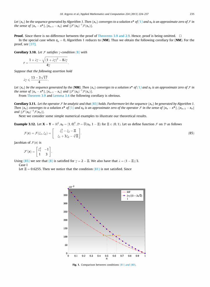
Fig. 1. Comparison between conditions (81) and (80).
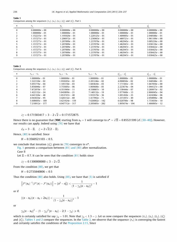
Table 1Comparison among the sequences frng; fsng; ftng; fs1
ng and ft1ng. Part I.
n rn sn tn t1n s1
n
0 0:000000eþ 00 0:000000eþ 00 0:000000eþ 00 0:000000eþ 00 0:000000eþ 001 1:000000e� 01 1:000000e� 01 1:000000e� 01 1:000000e� 01 1:000000e� 012 1:152215e� 01 1:195920e� 01 1:220125e� 01 1:409005e� 01 2:940588e� 013 1:157271e� 01 1:206972e� 01 1:236963e� 01 1:480721e� 01 1:961109eþ 004 1:157277e� 01 1:207009e� 01 1:237070e� 01 1:482945e� 01 3:005236eþ 005 1:157277e� 01 1:207009e� 01 1:237070e� 01 1:482947e� 01 3:038136eþ 006 1:157277e� 01 1:207009e� 01 1:237070e� 01 1:482947e� 01 3:038422eþ 007 1:157277e� 01 1:207009e� 01 1:237070e� 01 1:482947e� 01 3:038425eþ 008 1:157277e� 01 1:207009e� 01 1:237070e� 01 1:482947e� 01 3:038425eþ 009 1:157277e� 01 1:207009e� 01 1:237070e� 01 1:482947e� 01 3:038425eþ 00
Table 2Comparison among the sequences frng; fsng; ftng; fs1
ng and ft1ng. Part II.
n rnþ1 � rn snþ1 � sn tnþ1 � tn t1nþ1 � t1
n s1nþ1 � s1
n
0 1:000000e� 01 1:000000e� 01 1:000000e� 01 1:000000e� 01 1:000000e� 011 1:522150e� 02 1:959203e� 02 2:201246e� 02 4:090050e� 02 1:940588e� 012 5:055776e� 04 1:105150e� 03 1:683820e� 03 7:171583e� 03 1:667050eþ 003 5:856846e� 07 3:755605e� 06 1:069600e� 05 2:223674e� 04 1:044127eþ 004 7:872070e� 13 4:351969e� 11 4:338887e� 10 2:138444e� 07 3:289973e� 025 1:422132e� 24 5:843899e� 21 7:140132e� 19 1:977660e� 13 2:866045e� 046 4:641326e� 48 1:053747e� 40 1:933579e� 36 1:691450e� 25 2:424286e� 067 4:943634e� 95 3:426132e� 80 1:417992e� 71 1:237297e� 49 2:050096e� 088 5:608605e� 189 3:621924e� 159 7:626002e� 142 6:620700e� 98 1:733659e� 109 7:218912e� 377 4:047712e� 317 2:205685e� 282 1:895674e� 194 1:466065e� 12
236 I.K. Argyros et al. / Applied Mathematics and Computation 224 (2013) 224–237
kc ¼ 0:171583417 > 3� 2ffiffiffi2p¼ 0:171572875:
Hence there is no guarantee that (NM) starting from x0 ¼ 1 will converge to xH ¼ffiffiffiffiN3p¼ 0:85521599 (cf. [30–40]). However,
our results can apply. Indeed using (76) we have that
L0 ¼ 3� N; n ¼ 2ffiffiffi2pð2� NÞ:
Hence, (80) is satisfied. Since
H ¼ 0:3560521103 < 0:5;
we conclude that iteration fs1ng given in (78) converges to xH.
Fig. 1 presents a comparison between (81) and (80) after normalization.Case IILet N ¼ 0:7. It can be seen that the condition (81) holds since
kc ¼ 0:1300000000 6 3� 2ffiffiffi2p
:
From the condition (80), we get that
H ¼ 0:2735840806 < 0:5
Thus the condition (80) also holds. Using (85), we have that (5) is satisfied if
F0ðx0Þ�1 F0ðxÞ � F 0ðx0Þð Þ��� ��� ¼ kx2 � x2
0k <1
ð1� c0kx� x0kÞ2� 1
or if
kðx� x0Þðx� x0 þ 2x0Þk <1
ð1� c0kx� x0kÞ2� 1
or
c0kx� x0k2 � ð1� c0Þ2kx� x0k � 2ð1� c0ÞP 0;
which is certainly satisfied for say c0 ¼ 1:01. Note that c0 < 1:3 ¼ c. Let us now compare the sequences frng; fsng; ftng; fs1ng
and ft1ng. Tables 1 and 2 compare the sequences. In the Table 2, we observe that the sequence frng is converging the fastest
and certainly satisfies the conditions of the Proposition 2.11, Since
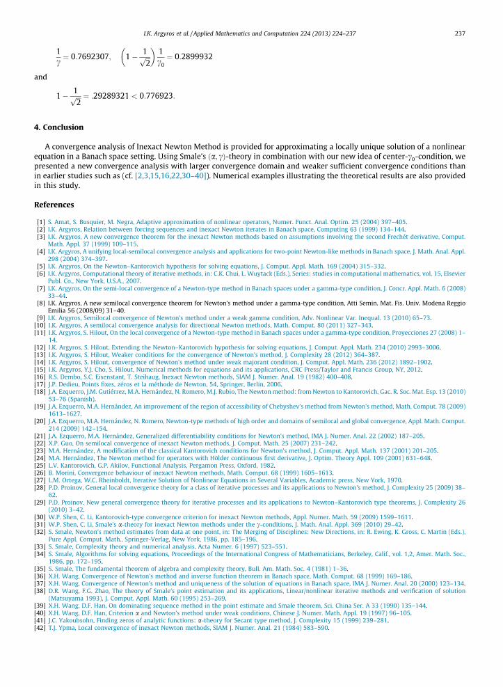
I.K. Argyros et al. / Applied Mathematics and Computation 224 (2013) 224–237 237
1c¼ 0:7692307; 1� 1ffiffiffi
2p
� �1c0¼ 0:2899932
and
1� 1ffiffiffi2p ¼ :29289321 < 0:776923:
4. Conclusion
A convergence analysis of Inexact Newton Method is provided for approximating a locally unique solution of a nonlinearequation in a Banach space setting. Using Smale’s ða; cÞ-theory in combination with our new idea of center-c0-condition, wepresented a new convergence analysis with larger convergence domain and weaker sufficient convergence conditions thanin earlier studies such as (cf. [2,3,15,16,22,30–40]). Numerical examples illustrating the theoretical results are also providedin this study.
References
[1] S. Amat, S. Busquier, M. Negra, Adaptive approximation of nonlinear operators, Numer. Funct. Anal. Optim. 25 (2004) 397–405.[2] I.K. Argyros, Relation between forcing sequences and inexact Newton iterates in Banach space, Computing 63 (1999) 134–144.[3] I.K. Argyros, A new convergence theorem for the inexact Newton methods based on assumptions involving the second Frechét derivative, Comput.
Math. Appl. 37 (1999) 109–115.[4] I.K. Argyros, A unifying local-semilocal convergence analysis and applications for two-point Newton-like methods in Banach space, J. Math. Anal. Appl.
298 (2004) 374–397.[5] I.K. Argyros, On the Newton–Kantorovich hypothesis for solving equations, J. Comput. Appl. Math. 169 (2004) 315–332.[6] I.K. Argyros, Computational theory of iterative methods, in: C.K. Chui, L. Wuytack (Eds.), Series: studies in computational mathematics, vol. 15, Elsevier
Publ. Co., New York, U.S.A., 2007.[7] I.K. Argyros, On the semi-local convergence of a Newton-type method in Banach spaces under a gamma-type condition, J. Concr. Appl. Math. 6 (2008)
33–44.[8] I.K. Argyros, A new semilocal convergence theorem for Newton’s method under a gamma-type condition, Atti Semin. Mat. Fis. Univ. Modena Reggio
Emilia 56 (2008/09) 31–40.[9] I.K. Argyros, Semilocal convergence of Newton’s method under a weak gamma condition, Adv. Nonlinear Var. Inequal. 13 (2010) 65–73.
[10] I.K. Argyros, A semilocal convergence analysis for directional Newton methods, Math. Comput. 80 (2011) 327–343.[11] I.K. Argyros, S. Hilout, On the local convergence of a Newton-type method in Banach spaces under a gamma-type condition, Proyecciones 27 (2008) 1–
14.[12] I.K. Argyros, S. Hilout, Extending the Newton–Kantorovich hypothesis for solving equations, J. Comput. Appl. Math. 234 (2010) 2993–3006.[13] I.K. Argyros, S. Hilout, Weaker conditions for the convergence of Newton’s method, J. Complexity 28 (2012) 364–387.[14] I.K. Argyros, S. Hilout, convergence of Newton’s method under weak majorant condition, J. Comput. Appl. Math. 236 (2012) 1892–1902.[15] I.K. Argyros, Y.J. Cho, S. Hilout, Numerical methods for equations and its applications, CRC Press/Taylor and Francis Group, NY, 2012.[16] R.S. Dembo, S.C. Eisenstant, T. Steihaug, Inexact Newton methods, SIAM J. Numer. Anal. 19 (1982) 400–408.[17] J.P. Dedieu, Points fixes, zéros et la méthode de Newton, 54, Springer, Berlin, 2006.[18] J.A. Ezquerro, J.M. Gutiérrez, M.A. Hernández, N. Romero, M.J. Rubio, The Newton method: from Newton to Kantorovich, Gac. R. Soc. Mat. Esp. 13 (2010)
53–76 (Spanish).[19] J.A. Ezquerro, M.A. Hernández, An improvement of the region of accessibility of Chebyshev’s method from Newton’s method, Math. Comput. 78 (2009)
1613–1627.[20] J.A. Ezquerro, M.A. Hernández, N. Romero, Newton-type methods of high order and domains of semilocal and global convergence, Appl. Math. Comput.
214 (2009) 142–154.[21] J.A. Ezquerro, M.A. Hernández, Generalized differentiability conditions for Newton’s method, IMA J. Numer. Anal. 22 (2002) 187–205.[22] X.P. Guo, On semilocal convergence of inexact Newton methods, J. Comput. Math. 25 (2007) 231–242.[23] M.A. Hernández, A modification of the classical Kantorovich conditions for Newton’s method, J. Comput. Appl. Math. 137 (2001) 201–205.[24] M.A. Hernández, The Newton method for operators with Hölder continuous first derivative, J. Optim. Theory Appl. 109 (2001) 631–648.[25] L.V. Kantorovich, G.P. Akilov, Functional Analysis, Pergamon Press, Oxford, 1982.[26] B. Morini, Convergence behaviour of inexact Newton methods, Math. Comput. 68 (1999) 1605–1613.[27] L.M. Ortega, W.C. Rheinboldt, Iterative Solution of Nonlinear Equations in Several Variables, Academic press, New York, 1970.[28] P.D. Proinov, General local convergence theory for a class of iterative processes and its applications to Newton’s method, J. Complexity 25 (2009) 38–
62.[29] P.D. Proinov, New general convergence theory for iterative processes and its applications to Newton–Kantorovich type theorems, J. Complexity 26
(2010) 3–42.[30] W.P. Shen, C. Li, Kantorovich-type convergence criterion for inexact Newton methods, Appl. Numer. Math. 59 (2009) 1599–1611.[31] W.P. Shen, C. Li, Smale’s a-theory for inexact Newton methods under the c-conditions, J. Math. Anal. Appl. 369 (2010) 29–42.[32] S. Smale, Newton’s method estimates from data at one point, in: The Merging of Disciplines: New Directions, in: R. Ewing, K. Gross, C. Martin (Eds.),
Pure Appl. Comput. Math., Springer-Verlag, New York, 1986, pp. 185–196.[33] S. Smale, Complexity theory and numerical analysis, Acta Numer. 6 (1997) 523–551.[34] S. Smale, Algorithms for solving equations, Proceedings of the International Congress of Mathematicians, Berkeley, Calif., vol. 1,2, Amer. Math. Soc.,
1986, pp. 172–195.[35] S. Smale, The fundamental theorem of algebra and complexity theory, Bull. Am. Math. Soc. 4 (1981) 1–36.[36] X.H. Wang, Convergence of Newton’s method and inverse function theorem in Banach space, Math. Comput. 68 (1999) 169–186.[37] X.H. Wang, Convergence of Newton’s method and uniqueness of the solution of equations in Banach space, IMA J. Numer. Anal. 20 (2000) 123–134.[38] D.R. Wang, F.G. Zhao, The theory of Smale’s point estimation and its applications, Linear/nonlinear iterative methods and verification of solution
(Matsuyama 1993), J. Comput. Appl. Math. 60 (1995) 253–269.[39] X.H. Wang, D.F. Han, On dominating sequence method in the point estimate and Smale theorem, Sci. China Ser. A 33 (1990) 135–144.[40] X.H. Wang, D.F. Han, Criterion a and Newton’s method under weak conditions, Chinese J. Numer. Math. Appl. 19 (1997) 96–105.[41] J.C. Yakoubsohn, Finding zeros of analytic functions: a-theory for Secant type method, J. Complexity 15 (1999) 239–281.[42] T.J. Ypma, Local convergence of inexact Newton methods, SIAM J. Numer. Anal. 21 (1984) 583–590.